Trans-Planckian Physics and the Spectrum of Fluctuations in a Bouncing Universe

Abstract

In this paper, we calculate the spectrum of scalar field fluctuations in a bouncing, asymptotically flat Universe, and investigate the dependence of the result on changes in the physics on length scales shorter than the Planck length which are introduced via modifications of the dispersion relation. In this model, there are no ambiguities concerning the choice of the initial vacuum state. We study an example in which the final spectrum of fluctuations depends sensitively on the modifications of the dispersion relation without needing to invoke complex frequencies. Changes in the amplitude and in the spectral index are possible, in addition to modulations of the spectrum. This strengthens the conclusions of previous work in which the spectrum of cosmological perturbations in expanding inflationary cosmologies was studied, and it was found that, for dispersion relations for which the evolution is not adiabatic, the spectrum changes from the standard prediction of scale-invariance.

I Introduction

The dependence of the spectrum of cosmological fluctuations in an inflationary Universe on hidden assumptions about the physics on length scales much smaller than the Planck length has been recently studied in Refs. BM1 ; MB2 ; N1 . A priori this dependence comes about since in typical scalar-field-driven inflationary models the duration of the period of expansion is so long that the physical wavelengths of comoving modes which correspond to the present large-scale structure of the Universe are much smaller than the Planck length at the beginning of inflation. In weakly coupled scalar field models of inflation, the spectrum of fluctuations is calculated by assuming that fluctuation modes start out in the vacuum (i.e. minimum energy density) state at the beginning of inflation and subsequently evolve as determined by the equations of motion. It is hence not unreasonable to expect that modifications of the physics on trans-Planckian scales could affect the final spectrum of fluctuations.

While the correct theory of trans-Planckian physics is not known, possible effects of the new physics can be modeled by changes in the dispersion relation of the fields corresponding to linear cosmological fluctuations. Such an approach was used earlier Unruh ; CJ to study the possible dependence of the spectrum of black hole radiation on trans-Planckian physics. Indeed, for a class of dispersion relations which deviate so strongly from the usual one such that the evolution of the mode functions is highly non-adiabatic and the effective frequency becomes imaginary, it was found that the spectrum of fluctuations is modified in a significant way compared to what is obtained for a linear dispersion relation BM1 ; MB2 . As shown in MB3 ; NP2 ; Starob , the final spectrum of fluctuations is unchanged if the change in the dispersion relation is not too drastic, the wave function evolves adiabatically, and hence the WKB approximation is valid throughout the evolution.

Two major deficiencies in the previous work concerned the choice of initial conditions and the fact that complex dispersion relations were required in order to obtain significant deviations from the standard results. In the previous papers, the assumption was made that the state starts out as the one minimizing the energy density. However, if the dispersion relation differs greatly from the linear one, in particular if it becomes complex, the physical motivation for choosing this state becomes unclear. This problem does not arise in a bouncing Universe. In this case, modes corresponding to present cosmological scales could well have had a physical wavelength smaller than the Planck length at the bounce point, but at early (pre-bounce) times, the wavelength was larger than the Planck length. In this context, initial conditions can be set up at some very early pre-bounce time during which the mode obeys a linear dispersion relation and the physical meaning of the minimum energy density state is clear. It is thus interesting to study the spectrum of fluctuations in a bouncing Universe which is asymptotically flat such that the choice of initial vacuum becomes unambiguous. It is also interesting to exhibit a case where complex dispersion relations are not needed. Although complex frequencies are standard in classical physics and in quantum mechanics, they seem to be more problematic in the context of quantum field theory.

In this article, we find an example of a bouncing Universe in which the spectrum of fluctuations depends sensitively on changes in the physics at length scales smaller than the Planck length, without requiring complex frequencies at high wavenumbers, thus improving on the second major deficiency of previous work. Another reason for investigating the dependence of the spectrum of fluctuations on modifications of trans-Planckian physics in a bouncing Universe is that one could expect (however, as we show, this is not correct) that the deviations in the spectrum incurred during the pre-bounce period when the wavelength is blue-shifting in the trans-Planckian regime will cancel with the deviation in the post-bounce trans-Planckian regime when the mode is being red-shifted. Such a result would then lead to the expectation that the results on the dependence of the spectrum of fluctuations on changes in the trans-Planckian physics might be different in the case of black holes and (non-bounce) inflationary cosmology. A third reason for analyzing a bouncing Universe is that there has recently been a lot of interest in the field of string cosmology in bouncing Universe models. In the Einstein frame, the pre-big-bang scenario PBB starts in a collapsing dilaton-dominated phase, and the same is true in the Ekpyrotic scenario KOST . Our arguments show that trans-Planckian effects could change the predictions of standard cosmological perturbation theory in these examples .

A model for the evolution of the scale factor in a bouncing inflationary Universe is $a(t)=a_{0}{\rm cosh}(Ht)$, where $a_{0}$ denotes the value of $a(t)$ at the center of the bounce, and $H$ is the Hubble expansion (contraction) rate during the period of exponential expansion (contraction). The idea of the calculation is to assume an initial spectrum of fluctuations at some early time $-t_{\rm f}$ when the wavelength of all modes of interest is much larger than the Planck length, to propagate the perturbation modes through the bounce and calculate the final spectrum at time $t_{\rm f}$. In this model, one of the difficulties encountered in the previous work BM1 ; MB2 , namely the problem of specifying the initial state in the trans-Planckian regime, is overcome. However, it is necessary now to set up initial conditions on wavelengths which typically also are much larger than the Hubble radius. The latter problem can be overcome by considering a bouncing Universe which is radiation-dominated in the asymptotic past and future, e.g. AS ; BD $a(\eta)=\sqrt{\alpha^{2}+\beta^{2}\eta^{2}}$, where $\alpha$ and $\beta$ are constants. Another toy model in which it is possible to set up well motivated initial conditions on scales much smaller than the Hubble radius and at the same time much larger than the Planck scale is a model in which the Universe is asymptotically flat both at large positive and negative times:

$$a(\eta)\,=\,\ell_{0}-{{\ell_{0}-\ell_{\rm b}}\over{1+(\eta/\eta_{0})^{2}}}\,$$ (1)

where $\ell_{0}$ and $\ell_{\rm b}$ (with $\ell_{\rm b}\ll\ell_{0}$) denote the asymptotic size of the Universe and the size at the bounce, respectively, and $\eta_{0}$ determines the time scale of the bounce, i.e. the time over which the scale factor changes. In the above, we are using conformal time $\eta$, and employing the convention that the scale factor carries dimension of length while the comoving coordinates (including conformal time) are dimensionless.

Finally, a comment is in order on the issue of backreaction. It has been shown in Refs. Tanaka ; Starob that the energy density of the particles created by trans-Planckian physics can contribute in a significant way to the background energy density. We do not address this interesting question since this clearly comes as a second step once a case where the spectrum is modified has been explicitly exhibited. In this paper we concentrate on the first question since it would be useless to treat the backreaction question if no well-motivated example where the spectrum is modified can be found. However, it should be clear that, once this is done (as shown in the present article), this problem becomes the central question in the study of trans-Planckian physics in cosmology.

This article is organized as follows. In section II, we review the arguments which show that no change in the final spectrum of fluctuations of a scalar matter field in a bouncing Universe is expected independent of the dispersion relation, provided that the WKB approximation remains justified. We give a qualitative reason to expect changes in the amplitude of the final spectrum for dispersion relations for which the adiabatic approximation breaks down. As mentioned above, our analysis assumes that perturbation theory remains justified and back-reaction can be neglected Tanaka . In Section III we study a concrete model, namely the asymptotically flat bouncing Universe given by (1) with a dispersion relation modified in the trans-Planckian regime according to the prescription of Corley and Jacobson CJ . We show that, as expected, both the overall amplitude and the shape of the spectrum differ from what is obtained for the linear dispersion relation, without ever requiring the effective frequency to become imaginary. The change in the spectrum is produced by an interesting combination of effects due to the modified dispersion relation and the driving term for Parker particle production Parker .

II Method and Qualitative Considerations

The equation of motion for a minimally coupled free scalar matter field $\Phi(\eta,\bbox{x})$ in a Universe with scale factor $a(\eta)$ in momentum space takes on the simple form

$$\mu^{\prime\prime}+\biggl{(}n^{2}-{{a^{\prime\prime}}\over a}\biggr{)}\mu\,=\,0\,,$$ (2)

making use of the re-scaling

$$\Phi(\eta,\bbox{x})\,=\,{1\over{(2\pi)^{3/2}}}\frac{1}{a(\eta)}\int{\rm d}\bbox{n}\mu(n,\eta)e^{i\bbox{n}\cdot\bbox{x}}\,,$$ (3)

where $\bbox{n}$ denotes the comoving wavenumber linked to the physical wavenumber by the relation $\bbox{k}=\bbox{n}/a(\eta)$. In the above, a prime denotes the derivative with respect to conformal time. The previous equations are valid for a spacetime with flat spatial sections. The advantage of considering a test scalar field and/or gravitational waves is that we do not need to address the origin of the dynamics of the scale factor. This is in contrast to the case of density perturbations. However, the Friedmann equation reads ${\cal H}^{2}/a^{2}+K/a^{2}=\kappa\sum_{i}\rho_{i}/3$, where ${\cal H}\equiv a^{\prime}/a$ and $\rho_{i}>0$ is the energy density. This means that a bounce is consistent with the Einstein equations only if $K=1$. For $K=0$, it would imply $\rho=0$ for each component. Therefore, it seems that it is inconsistent to use Eq. (2) if the scale factor behaves such that there is a bounce. There are two ways out of the previous argument. The first one is the following. If $K=1$, then Eq. (2) takes the form $\mu^{\prime\prime}+(n^{2}-K-a^{\prime\prime}/a)\mu=0$. In addition the eigenfunctions of the three-dimensional Laplacian operator are no longer planes waves. However, if we restrict ourselves to modes with wavelengths much smaller than the curvature radius, then they do not feel the curvature of the spacelike section and we can safely work with Eq. (2). It could be checked that this is indeed the case for the wavenumbers considered in the example presented in the following section. Another possibility is to use the “nonsingular Universe construction” bms . In this case, it is definitely possible to get a spatially flat bounce. What happens is that the higher derivative terms become important at the bounce and enable the evasion of the previous argument by supplying other terms in the analog of the first Friedmann equation. In conclusion, although in this article we consider a scale factor with a bounce, we can nevertheless work with Eq. (2), i.e. we let the nonsingular Universe construction enter only via the scale factor.

The method introduced in Unruh ; CJ to study the dependence of the spectrum of fluctuations on trans-Planckian physics is to replace the linear dispersion relation $\omega_{{}_{\bf phys}}=k$ by a non standard dispersion relation $\omega_{{}_{\bf phys}}=\omega_{{}_{\bf phys}}(k)$ where the function $\omega_{{}_{\bf phys}}(k)$ is a priori arbitrary. In the context of cosmology, it has been shown in Ref. BM1 ; MB2 that this amounts to replacing $n^{2}$ appearing in (2) with $n_{\rm eff}^{2}(n,\eta)$ defined by

$$n^{2}\,\rightarrow\,n_{\rm eff}^{2}(n,\eta)\equiv a^{2}(\eta)\omega_{{}_{\bf phys}}^{2}\biggl{[}\frac{n}{a(\eta)}\biggr{]}.$$ (4)

For a fixed comoving mode, this implies that the dispersion relation becomes time-dependent. Various forms for $n_{\rm eff}$ have been used, e.g.

$$n_{\rm eff}(n,\eta)=n{{\lambda(\eta)}\over{\ell_{{}_{\rm C}}}}{\rm tanh}^{1/p}\biggl{[}\biggl{(}{{\ell_{{}_{\rm C}}}\over{\lambda(\eta)}}\biggr{)}^{p}\biggr{]},\quad n_{\rm eff}^{2}(n,\eta)=n^{2}+n^{2}b_{m}\biggl{[}{{\ell_{{}_{\rm C}}}\over{\lambda(\eta)}}\biggr{]}^{2m},$$ (5)

the first being a generalization of the relation studied by Unruh Unruh whereas the second one is a generalization of the relations used by Corley and Jacobson CJ . In the above, $\lambda(\eta)$ is the physical wavelength, $\ell_{{}_{\rm C}}$ is the cutoff length (which can be taken to be the Planck length), $p$ and $m$ are integers, and $b_{m}$ is a real number which can be either positive or negative. Thus, the equation of motion to be analyzed is

$$\mu^{\prime\prime}+\biggl{[}n_{\rm eff}^{2}(n,\eta)-{{a^{\prime\prime}}\over a}\biggr{]}\mu\,=\,0\,.$$ (6)

For fixed comoving wavenumber $n$, the evolution of $\mu$ depends crucially on which region $\eta$ lies in. The first region is the trans-Planckian region with

$$\lambda(\eta)\,\ll\,\ell_{{}_{\rm C}}\,\,\,({\rm{Region\ \ 1}})\,.$$ (7)

Let us first consider the standard inflationary scale factor and a monotonic dispersion relation [like the first one in Eq. (5) or the second one with $b_{m}>0$]. This means that, initially, the term $n_{\rm eff}^{2}(n,\eta)$ dominates in Eq. (6). The initial conditions are fixed in this region and since the WKB approximation is applicable, we can choose the initial state as the “minimizing energy state” Brown78 . Then, the (positive frequency) solution is given by

$$\mu(\eta)\,\simeq\,\frac{1}{\sqrt{2n_{\rm eff}(n,\eta)}}\exp\biggl{[}-i\int_{\eta_{\rm i}}^{\eta}n_{\rm eff}{\rm d}\tau\biggr{]}\,,$$ (8)

where $\eta_{i}$ is some initial time.

The second region corresponds to

$$\lambda\,\gg\,\ell_{{}_{\rm C}}\,\,\,{\rm{and}}\,\,\,n^{2}\,\gg\,a^{\prime\prime}/a\,\,\,({\rm{Region\ \ 2}})\,.$$ (9)

In this region the mode has reached the linear part of the dispersion relation. The general solution in Region 2 is the plane wave

$$\mu\,=\,B_{1}\exp(-in\eta)+B_{2}\exp(in\eta)$$ (10)

with constant coefficients $B_{1}$ and $B_{2}$. For the standard dispersion relation, the initial conditions are fixed in this region. The usual choice of the vacuum state is $B_{1}=1/\sqrt{2n}$, $B_{2}=0$. In general $B_{1}$ and $B_{2}$ are determined by the matching conditions between Regions 1 and 2. However, if the dynamics is adiabatic throughout (in particular if the $a^{\prime\prime}/a$ term is negligible), the WKB approximation holds and the solution is always given by (8). Therefore, if we start with $B_{2}=0$ and uses this solution, one finds that $B_{2}$ remains zero at all times. Deep in the region where $n_{\rm eff}\simeq n$ the solution becomes

$$\mu(\eta)\simeq{1\over{\sqrt{2n}}}\exp(-i\phi-in\eta),$$ (11)

i.e. the standard vacuum solution times a phase which will disappear when we calculate the modulus. The phase $\phi$ is given by $\phi\equiv\int_{\eta_{\rm i}}^{\eta_{1}}n_{\rm eff}{\rm d}\tau$, where $\eta_{1}$ is the time at which $n_{\rm eff}\simeq n$.

The situation changes dramatically if we consider non-monotonic dispersion relations. This is the case if $b_{m}<0$ in Eq. (5) or for the dispersion relation introduced in Ref. Mersini . Two new features can occur. Either the dispersion relation can become complex (this is in general the case if $b_{m}<0$) or the term $a^{\prime\prime}/a$ dominates (this is the case for the dispersion relation introduced in Ref. Mersini or for the Corley/Jacobson dispersion relation with $b_{m}<0$ for a certain range of comoving wavenumbers). In this case, the WKB approximation is violated in Region 1 and we expect changes in the final spectrum. Unfortunately, in the context of the standard increasing inflationary scale factor, one also looses the ability to fix natural initial conditions. However, this is no longer true if the spacetime is asymptotically flat because then, at infinity, the term $a^{\prime\prime}/a$ goes to zero, see also Ref. LLMU . Therefore, in this case, we can choose well-motivated initial conditions. A good example of such a situation is provided by a bouncing Universe. From the above considerations, we expect that in this case the final spectrum is modified and the initial conditions can be fixed naturally. As an additional benefit, complex frequencies can be avoided. In the next section, we consider a toy model where these qualitative arguments can be implemented concretely, at the level of equations.

III A Specific Example

We will now illustrate the qualitative arguments of the previous section with a concrete quantitative example. We take the asymptotically flat bouncing Universe given by (1). We consider the type of modified dispersion relation for which in the case of an expanding inflationary Universe the deviations in the spectrum were found BM1 ; MB2 , namely the (generalization of the) Corley/Jacobson dispersion relation (5) with $b_{m}$ negative. In this case, $\omega_{{}_{\bf phys}}(k)$ is given by

$$\omega_{{}_{\bf phys}}^{2}(k)=k^{2}-|b_{m}|k^{2}\biggl{(}\frac{k^{2}}{k_{{}_{\rm C}}^{2}}\biggr{)}^{m},$$ (12)

where $k_{{}_{\rm C}}$ is the cutoff physical wavenumber. The dispersion relation is represented in Fig. 1.

Figure 1: Corley/Jacobson dispersion relation for $m=1$ and $|b_{m}|=1$. In general $\omega_{{}_{\bf phys}}^{2}(k)$ vanishes at $k=k_{{}_{\rm C}}|b_{m}|^{-1/(2m)}$. For $k>k_{{}_{\rm C}}|b_{m}|^{-1/(2m)}$, the physical frequency becomes imaginary.

The behavior of the solutions of the equation of motion $\mu^{\prime\prime}+\mu(n_{\rm eff}^{2}-a^{\prime\prime}/a)=0$ is determined by the competition between the two terms $n_{\rm eff}^{2}$ and $a^{\prime\prime}/a$ given by

$$n_{\rm eff}^{2}(n,\eta)\,=\,n^{2}-n^{2}\frac{|b_{m}|}{\ell_{{}_{\rm C}}^{-2m}}\biggl{(}\frac{n}{2\pi}\biggr{)}^{2m}\biggl{[}\ell_{0}-\frac{\ell_{0}-\ell_{\rm b}}{1+(\eta/\eta_{0})^{2}}\biggr{]}^{-2m},\quad\frac{a^{\prime\prime}}{a}=\frac{2(\ell_{0}-\ell_{\rm b})}{\eta_{0}^{2}\ell_{\rm b}}\frac{1-3(\eta/\eta_{0})^{2}}{[1+(\eta/\eta_{0})^{2}]^{3}},$$ (13)

where $\ell_{{}_{\rm C}}\equiv 1/k_{{}_{\rm C}}$ is the cutoff length. These two terms are represented in Fig. 2. When $n_{\rm eff}^{2}>a^{\prime\prime}/a$, which is always the case when $\eta/\eta_{0}\rightarrow\pm\infty$, the WKB approximation is valid and the fundamental solutions can be written as

$$\mu\simeq\frac{1}{\sqrt{2n_{\rm eff}}}\exp\biggl{[}\pm i\int^{\eta}n_{\rm eff}(n,\tau){\rm d}\tau\biggr{]}\rightarrow_{\eta/\eta_{0}\rightarrow\pm\infty}\frac{1}{\sqrt{2n}}e^{\pm in\eta}.$$ (14)

In this case, the physical wavenumbers of the modes are such that they correspond to the linear part of the dispersion relation, see Fig. 1. In this situation, natural initial conditions can be chosen. Note that these initial conditions are, in a sense, even “more standard” than in the previous studies on trans-Planckian physics since usually the initial conditions are set in a region where the dispersion relation is not linear (but, as explained above, since the WKB approximation holds, meaningful initial conditions can nevertheless be considered). On the contrary, when $n_{\rm eff}^{2}<a^{\prime\prime}/a$ the WKB approximation is violated and two independent solutions are given by

$$\mu\simeq a(\eta),\quad\mu\simeq a(\eta)\int^{\eta}\frac{{\rm d}\tau}{a^{2}({\tau})}.$$ (15)

In this case, we are close to the cutoff scale and $\omega_{{}_{\bf phys}}^{2}(k)$ being close to zero, see Fig. 1, the $a^{\prime\prime}/a$ term dominates. This situation is very similar to the one discussed in Ref. Mersini where this part of the dispersion relation has been named “the tail”. In fact, it is possible to quantify exactly the accuracy of the WKB approximation. Given an equation of the form $\mu^{\prime\prime}+\omega^{2}\mu=0$, the WKB approximation is valid if the quantity $|Q/\omega^{2}|\ll 1$, where the quantity $Q$ is defined by the following expression

$$Q=\frac{3(\omega^{\prime})^{2}}{4\omega^{2}}-\frac{\omega^{\prime\prime}}{2\omega}.$$ (16)

This standard criterion can be obtained in the following manner. The WKB solution, $\mu_{\rm wkb}$, satisfies the equation $\mu_{\rm wkb}^{\prime\prime}+\mu_{\rm wkb}(\omega^{2}-Q)=0$ exactly. Therefore, one has $\mu\simeq\mu_{\rm wkb}$ if $|Q/\omega^{2}|\ll 1$. In the present context, $\omega^{2}$ is of course equal to $n_{\rm eff}^{2}-a^{\prime\prime}/a$. We have plotted the quantity $|Q/\omega^{2}|$ in Fig. 3. When $|\eta/\eta_{0}|\gg 1$, $|Q/\omega^{2}|\ll 1$ and the WKB approximation is satisfied, as expected from the previous discussion. The quantity $|Q/\omega^{2}|$ increases when one approaches the bounce. At $\eta=\eta_{\rm j}$, where $\omega(\eta_{\rm j})=0$, there is a divergence. This point is a turning point. Then for $|\eta/\eta_{0}|\ll 1$, as can be seen in Fig. 3, $|Q/\omega^{2}|$ remains large and the WKB approximation breaks down in agreement with the considerations above.

Figure 2: The solid curve is $a^{\prime\prime}/a$, the dashed one $n^{2}_{\rm eff}$. The values used are $\ell_{0}=5000$, $\ell_{\rm b}=10$, $\ell_{{}_{\rm C}}=1$, $|b_{m}|=1$, $m=1$ and $n=60$.

Figure 3: Absolute value of Q versus conformal time. The values used are $\ell_{0}=5000$, $\ell_{\rm b}=10$, $\ell_{{}_{\rm C}}=1$, $|b_{m}|=1$, $m=1$ and $n=55$.

In a bouncing Universe, the modes start in the linear part of the dispersion relation, pass through the non-linear part and then come back in the standard region. However, things are not so simple because there exists a range of comoving wavenumbers such that the dispersion relation becomes complex. Although this case is a priori interesting, it clearly requires more speculative considerations, in particular the quantization in the presence of imaginary frequency modes. Since our goal in this paper is to exhibit a case where everything can be done in a standard manner, we will restrict ourselves to modes which never enter the region where the dispersion relation becomes complex. In the following, we determine the range of comoving wavenumbers we are interested in and for which we are going to calculate the power spectrum.

The maximum of the absolute value of $a^{\prime\prime}/a$ is located at $\eta=0$ and is given by $(2/\eta_{0}^{2})(\ell_{0}/\ell_{\rm b}-1)$. Therefore, if we restrict ourselves to modes such that

$$n\,\gg\,n_{\rm b}\equiv\frac{\sqrt{2}}{\eta_{0}}\biggl{(}\frac{\ell_{0}}{\ell_{\rm b}}-1\biggr{)}^{1/2},$$ (17)

then one is sure that, with an unmodified dispersion relation, the term $a^{\prime\prime}/a$ can always be neglected and that the initial spectrum is never changed. Clearly, this is not a physical restriction but it renders the comparison with the case with a modified dispersion relation easier. The minimum of the modified part of the dispersion relation is given by (from now on, we consider the case $|b_{m}|=1$ and $m=1$ since it is more convenient and does not restrict the physical content of the problem in any way)

$$n_{\rm eff}^{2}(n,\eta=0)=n^{2}\biggl{[}1-\biggl{(}\frac{n}{n_{\rm inf}}\biggr{)}^{2}\biggr{]},\quad n_{\rm inf}\equiv 2\pi\frac{\ell_{\rm b}}{\ell_{{}_{\rm C}}}.$$ (18)

Therefore, to maintain a real dispersion relation, we should only consider modes such that $n<n_{\rm inf}$. Of course, for consistency, the parameters of the model must be chosen such that $n_{\rm b}<n_{\rm inf}$. This is the case for the most natural choice, i.e., $\ell_{0}\gg\ell_{\rm b}\gg\ell_{{}_{\rm C}}$. In the following, as already mentioned above, the time $\eta_{\rm j}(n)$ such that

$$n_{\rm eff}^{2}(n,\eta_{\rm j})\,=\,{{a^{\prime\prime}}\over a}$$ (19)

will play a crucial role. For convenience we will only consider values of $n$ such that this time is determined only by the central peak of $a^{\prime\prime}/a$ and not by the two wings. In practice, this amounts to taking $n_{\rm eff}^{2}(n,\infty)>n_{\rm b}^{2}/4$ since $n_{\rm b}^{2}/4$ is the maximum height of the wings. Then it is easy to show that $n^{2}\in[n_{-}^{2},n_{+}^{2}]$ where

$$n_{\pm}^{2}=\frac{n_{\rm sup}^{2}}{2}\ \biggl{(}1\pm\sqrt{1-\frac{n_{\rm b}^{2}}{n_{\rm sup}^{2}}}\biggr{)},$$ (20)

where $n_{\rm sup}\equiv 2\pi\ell_{0}/\ell_{{}_{\rm C}}$ is the largest value of $n$ such that $n_{\rm eff}^{2}(n,\infty)$ remains real. Therefore, the range we are interested in is given by

$$\max(n_{\rm b}^{2},n_{-}^{2})<n^{2}<\min(n_{\rm inf}^{2},n_{+}^{2}).$$ (21)

In practice, we have $n_{-}^{2}\simeq(1/4)n_{\rm b}^{2}$ and $n_{+}^{2}\simeq n_{\rm sup}^{2}$. This means that $\max(n_{\rm b}^{2},n_{-}^{2})=n_{\rm b}^{2}$, $\min(n_{\rm inf}^{2},n_{+}^{2})=n_{\rm inf}^{2}$ and that the range reduces to

$$n_{\rm b}^{2}\,<n^{2}\,<\,n_{\rm inf}^{2}\,.$$ (22)

Having determined the relevant wavenumbers, we can now choose the initial condition and solve the equation of motion. In the first region where $\eta<-\eta_{\rm j}(n)$, we only consider positive frequency modes and we have

$$\mu_{\rm I}(\eta)=\frac{1}{\sqrt{2n_{\rm eff}}}\exp\biggl{[}-i\int^{\eta}_{\eta_{\rm i}}n_{\rm eff}(n,\tau){\rm d}\tau\biggr{]},$$ (23)

where $\eta_{\rm i}$ is an arbitrary initial time. In the second region, where $-\eta_{\rm j}(n)<\eta<\eta_{\rm j}(n)$, the solution is given by

$$\mu_{\rm II}(\eta)=B_{1}a(\eta)+B_{2}a(\eta)\int_{0}^{\eta}\frac{{\rm d}\tau}{a^{2}({\tau})}.$$ (24)

The lower bound of the integral is a priori arbitrary. However, it is very convenient to take it equal to zero because in this case the second branch becomes odd whereas the first one (i.e. the scale factor) is even. Then, it is easy to show that

$$\int_{0}^{\eta}\frac{{\rm d}\tau}{a^{2}({\tau})}=\frac{\eta_{0}}{\ell_{\rm b}^{2}}\biggl{\{}\frac{1}{p^{2}}\frac{\eta}{\eta_{0}}+\frac{1-2p+p^{2}}{2p^{2}[1+p(\eta/\eta_{0})^{2}]}\frac{\eta}{\eta_{0}}+\frac{p^{2}+2p-3}{2p^{5/2}}\arctan\biggl{(}\sqrt{p}\frac{\eta}{\eta_{0}}\biggr{)}\biggr{\}},$$ (25)

where $p\equiv\ell_{0}/\ell_{\rm b}$. Finally, the solution in the third region where $\eta>\eta_{\rm j}(n)$ can be written as

$$\mu_{\rm III}(\eta)=\frac{C_{1}}{\sqrt{2n_{\rm eff}}}\exp\biggl{[}-i\int^{\eta}_{\eta_{\rm i}}n_{\rm eff}(n,\tau){\rm d}\tau\biggr{]}+\frac{C_{2}}{\sqrt{2n_{\rm eff}}}\exp\biggl{[}+i\int^{\eta}_{\eta_{\rm i}}n_{\rm eff}(n,\tau){\rm d}\tau\biggr{]}.$$ (26)

The goal is now to calculate the coefficients $C_{1}$ and $C_{2}$. Using the continuity of the mode function $\mu$ and of its derivative, we find

$$C_{1}(n) = \frac{i}{2W[-\eta_{j}(n)]}\frac{e^{i[\Omega(\eta_{\rm j})-\Omega(-\eta_{\rm j})]}}{\sqrt{n_{\rm eff}(n,-\eta_{\rm j})n_{\rm eff}(n,\eta_{\rm j})}}\biggl{\{}-[g^{\prime}+\alpha g](-\eta_{\rm j})[f^{\prime}+\bar{\alpha}f](\eta_{\rm j})+[f^{\prime}+\alpha f](-\eta_{\rm j})[g^{\prime}+\bar{\alpha}g](\eta_{\rm j})\biggr{\}},$$ (27)

$$C_{2}(n) = \frac{-i}{2W[-\eta_{j}(n)]}\frac{e^{-i[\Omega(\eta_{\rm j})+\Omega(-\eta_{\rm j})]}}{\sqrt{n_{\rm eff}(n,-\eta_{\rm j})n_{\rm eff}(n,\eta_{\rm j})}}\biggl{\{}-[g^{\prime}+\alpha g](-\eta_{\rm j})[f^{\prime}+\alpha f](\eta_{\rm j})+[f^{\prime}+\alpha f](-\eta_{\rm j})[g^{\prime}+\alpha g](\eta_{\rm j})\biggr{\}},$$ (28)

where we have used the short-hand notation $f\equiv a(\eta)$ and $g\equiv a(\eta)\int^{\eta}_{0}{\rm d}\tau/a^{2}(\tau)$. We have also utilized the following definitions: $W\equiv gf^{\prime}-g^{\prime}f$ is the Wronskian, $\Omega(\eta)\equiv\int^{\eta}_{\eta_{\rm i}}n_{\rm eff}(n,\tau){\rm d}\tau$, and the quantity $\alpha$ is

$$\alpha\equiv\frac{n_{\rm eff}^{\prime}}{2n_{\rm eff}}+in_{\rm eff}.$$ (29)

Using the fact that $n_{\rm eff}$ is even, it is easy to see that $\alpha(n,-\eta)=-\bar{\alpha}(n,\eta)$. Using the same property, one could also simplify the factor $\sqrt{n_{\rm eff}(n,-\eta_{\rm j})n_{\rm eff}(n,\eta_{\rm j})}=n_{\rm eff}(n,\eta_{\rm j})$ in the above equation. The final result is given by Eqs. (27), (28) where all the functions are explicitly known except the function $\eta_{\rm j}=\eta_{\rm j}(n)$. The dependence on the dispersion relation of the final result is completely encoded in this function. The time $\eta_{\rm j}(n)$ is the solution of an algebraic equation that is not possible to solve explicitly. However, we can find an approximation if the function $n_{\rm eff}(n,\eta)$ is Taylor expanded around $\eta=0$. For the function $a^{\prime\prime}/a$ , we use a quadratic least square approximation which gives a better result. We obtain

$$n_{\rm eff}^{2}(n,\eta)\simeq n^{2}-n^{2}\biggl{(}\frac{n}{n_{\rm inf}}\biggr{)}^{2}(1-n_{\rm b}^{2}\eta^{2}),\quad\frac{a^{\prime\prime}}{a}\simeq n_{\rm b}^{2}\biggl{[}1-6\biggl{(}\frac{\eta}{\eta_{0}}\biggr{)}^{2}\biggr{]}.$$ (30)

The two functions and their approximations are represented in Fig. 4. We see now that $\eta_{\rm j}(n)$ is the solution of a quadratic algebraic equation. Straightforward calculations give

$$\eta_{\rm j}^{2}(n)\simeq\frac{n^{2}}{n_{\rm b}^{2}}\biggl{[}\biggl{(}\frac{n}{n_{\rm inf}}\biggr{)}^{2}+\biggl{(}\frac{n_{\rm b}}{n}\biggr{)}^{2}-1\biggr{]}\biggl{[}n^{2}\biggl{(}\frac{n}{n_{\rm inf}}\biggr{)}^{2}+\frac{6}{\eta_{0}^{2}}\biggr{]}^{-1}.$$ (31)

The function $\eta_{\rm j}(n)$ can also be found exactly by numerical calculations.

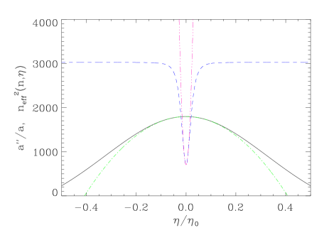
Figure 4: The solid curve represents $a^{\prime\prime}/a$, the dot-dashed curve its quadratic approximation. The dashed curve represents $n^{2}_{\rm eff}$, and its quadratic approximation is the fourth curve. Values chosen are $\ell_{0}=5000$, $\ell_{\rm b}=10$, $\ell_{{}_{\rm C}}=1$, $|b_{m}|=1$, $m=1$ and $n=60$.

We have done this computation by means of a Fortran code. The comparison of the exact result with its approximation given in Eq. (31) is represented in Fig. 5. The function $n_{\rm eff}(n,\eta=0)$ is not monotonic and has a maximum around $n\simeq 45$ for the values of the parameters considered in Fig. 5. For this value $n_{\rm eff}(n,\eta)$ is almost never smaller than $a^{\prime\prime}/a$. It is clear that around this value the approximation will be very good whereas for other values of $n$, especially for $n\simeq n_{\rm b}$, the approximation will be less good. This is due to the fact that when $n$ approaches $n_{\rm b}$, the asymptotic value of $n_{\rm eff}(n,\eta)$ decreases and the curve opens out at the intersection with $a^{\prime\prime}/a$. As a consequence, the quadratic approximation employed above breaks down. This is confirmed by the plots in Fig. 5. The approximation can be less good for other values of the parameters.

From the above analysis, it is clear that $\epsilon\equiv\eta_{\rm j}(n)/\eta_{0}$ is a small number. We can therefore expand everything in terms of the parameter $\epsilon$. This will allow us to get an analytical estimate of the spectrum. After tedious but straightforward computations, one obtains the following expressions for the coefficients $C_{1}(n)$ and $C_{2}(n)$

$$C_{1}(n) = 1+\epsilon\frac{i\eta_{0}}{2n}\biggl{[}2n^{2}\biggl{(}1-\frac{n^{2}}{n_{\rm inf}^{2}}\biggr{)}^{1/2}+n_{\rm b}^{2}\biggl{(}1-\frac{n^{2}}{n_{\rm inf}^{2}}\biggr{)}^{-1/2}+n_{\rm b}^{2}\biggl{(}1-\frac{n^{2}}{n_{\rm inf}^{2}}\biggr{)}^{-3/2}\biggr{]}+{\cal O}(\epsilon^{2}),$$ (32)

$$C_{2}(n) = -\epsilon\frac{i\eta_{0}}{2n}e^{-2i\Psi_{\rm i}(n)}\biggl{[}2n^{2}\biggl{(}1-\frac{n^{2}}{n_{\rm inf}^{2}}\biggr{)}^{1/2}+n_{\rm b}^{2}\biggl{(}1-\frac{n^{2}}{n_{\rm inf}^{2}}\biggr{)}^{-1/2}+n_{\rm b}^{2}\biggl{(}1-\frac{n^{2}}{n_{\rm inf}^{2}}\biggr{)}^{-3/2}\biggr{]}+{\cal O}(\epsilon^{2}),$$ (33)

where $\Psi_{\rm i}(n)\equiv\int_{\eta_{\rm i}}^{0}n_{\rm eff}(n,\tau){\rm d}\tau$. Several comments are in order at this point. Firstly, the expressions of the two coefficients have exactly the expected form. When the parameter $\epsilon$ goes to zero, $C_{1}(n)$ goes to one and $C_{2}(n)$ goes to zero, i.e., we recover an unmodified spectrum. This is in complete agreement with the fact that, when $\epsilon=\eta_{\rm j}(n)/\eta_{0}\rightarrow 0$, the effective wavenumber $n_{\rm eff}$ never penetrates the region where the WKB approximation is violated. This is in this sense that the parameter $\epsilon$ is the relevant parameter to expand the spectrum in since it is clearly directly linked to the violation of the WKB approximation. Therefore, in the limit $\epsilon\rightarrow 0$, one recovers the usual spectrum. Secondly, it is interesting to notice that the two terms proportional to $\epsilon$ in $C_{1}(n)$ and $C_{2}(n)$ are the same up to a global phase. To compute the phase in Eqs. (27) and (28), we have written $\Omega(\eta)=\Psi_{\rm i}(n)+\int_{0}^{\eta}n_{\rm eff}(n,\tau){\rm d}\tau$. Since we only need to evaluate $\Omega(\pm\eta_{\rm j})$, one can use the approximate equation for $n_{\rm eff}$, see Eq. (30), in the integral $\int_{0}^{\eta_{\rm j}}n_{\rm eff}(n,\tau){\rm d}\tau$. One finds

$$\Omega(\pm\eta_{\rm j})=\Psi_{\rm i}\pm\epsilon n\eta_{0}\biggl{(}1-\frac{n^{2}}{n_{\rm inf}^{2}}\biggr{)}^{1/2}+{\cal O}(\epsilon^{3}).$$ (34)

Let us remark that the term $e^{-i[\Omega(\eta_{\rm j})+\Omega(-\eta_{\rm j})]}$ in the expression of $C_{2}(n)$ does not contribute to order $\epsilon$ whereas the factor $e^{i[\Omega(\eta_{\rm j})-\Omega(-\eta_{\rm j})]}$ gives a contribution at this order. This contribution is exactly such that the two terms proportional to $\epsilon$ in Eqs. (32), (33) have the same absolute value. Thirdly, the factor $1-n^{2}/n_{\rm inf}^{2}$ is always positive since we restrict ourselves to the regime where $n^{2}<n_{\rm inf}^{2}$. Therefore, the above expressions of $C_{1}(n)$ and $C_{2}(n)$ are always well-defined. Finally, interestingly enough, the two coefficients $C_{1}(n)$ and $C_{2}(n)$ have a similar structure to one of the corresponding coefficients found in Ref. LLMU where another example of a modified spectrum has been exhibited.

We are now in a position where we can calculate the spectrum explicitly. It is defined by the following equation

$$n^{3}P(n)\propto n^{3}\biggl{|}\frac{\mu}{a}\biggr{|}^{2}.$$ (35)

We will evaluate the spectrum in the region where $\eta/\eta_{0}\gg 1$. In this case, $a(\eta)\simeq\ell_{0}$ and $n_{\rm eff}\simeq n$. Expanding everything in terms of the small parameter $\epsilon$, one obtains

$$n^{3}P(n) \propto \frac{n^{2}}{2\ell_{0}^{2}}+\epsilon\frac{\eta_{0}}{2\ell_{0}^{2}}n\biggl{[}2n^{2}\biggl{(}1-\frac{n^{2}}{n_{\rm inf}^{2}}\biggr{)}^{1/2}+n_{\rm b}^{2}\biggl{(}1-\frac{n^{2}}{n_{\rm inf}^{2}}\biggr{)}^{-1/2}+n_{\rm b}^{2}\biggl{(}1-\frac{n^{2}}{n_{\rm inf}^{2}}\biggr{)}^{-3/2}\biggr{]}$$ (36)

$$\times\sin\biggl{[}2\Phi(n)-2\Psi_{\rm i}(n)+2n(\eta-\eta_{+})\biggr{]}+{\cal O}(\epsilon^{2}),$$

where $\eta_{+}>\eta_{\rm j}$ is the time at which $n_{\rm eff}\simeq n$ and the phase $\Phi(n)$ is defined by $\Phi(n)\equiv\int_{\eta_{\rm i}}^{\eta_{+}}{\rm d}\tau n_{\rm eff}$. Again the spectrum has the expected form. The leading order is the vacuum spectrum with spectral index $3$ and the next-to-leading order (proportional to $\epsilon$) has the form of a complicated function of $n$ times superimposed oscillations. We have plotted this complicated function (without the superimposed oscillations) in Fig. 6.

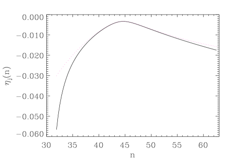
Figure 5: The dependence of the matching time $\eta_{\rm j}(n)$ on the wave number $n$ for the values $\ell_{0}=5000$, $\ell_{\rm b}=10$, $\ell_{{}_{\rm C}}=1$, $|b_{m}|=1$, $m=1$. The solid curve is the exact result determined numerically, the dotted curve is obtained using the analytical approximations.

We can check that the correction remains small and that, therefore, the approximation employed in this article is consistent. On the other hand, when the wavenumber $n$ approaches $n_{\rm inf}$, the approximation scheme breaks down but, precisely in this limit, the whole problem becomes pointless in agreement with the considerations above. We also see that the deviation is minimum around $n\simeq 45$ (for these values of the parameters) because, as already mentioned above, in this case the term $a^{\prime\prime}/a$ almost never dominates. Although the present example is only a toy model, it is quite interesting to see that it bears some close resemblance with the other example of a modified spectrum found in Ref. LLMU . This suggests that the features previously exhibited may be valid in general.

We have thus reached our main goal: find an example where the initial conditions can be fixed naturally, where the frequency never becomes complex and where the final spectrum is modified. Note that in this example, the change in the spectrum comes about from an interplay between the modified dispersion relation factor $n^{2}_{\rm eff}$ and the factor $a^{\prime\prime}/a$ which is responsible for Parker particle production Parker . For an unmodified linear dispersion relation, the $a^{\prime\prime}/a$ term is always negligible and there is no particle production. However, for our modified dispersion relation, for a range of modes the Parker particle production term becomes important and leads to non-adiabatic evolution. The length of time during which the $a^{\prime\prime}/a$ term dominates depends on the specifics of the dispersion relation, and hence the final spectrum will depend on these specifics.

Figure 6: Amplitude of the next-to-leading order correction to the spectrum without the superimposed oscillations. Values chosen are $\ell_{0}=5000$, $\ell_{\rm b}=10$, $\ell_{{}_{\rm C}}=1$, $|b_{m}|=1$, $m=1$. When $n$ approaches $n_{\rm inf}$ the correction blows up and the approximation becomes meaningless.

IV Discussion

In this paper we have studied the dependence of the spectrum of a free scalar field in a bouncing Universe on trans-Planckian effects introduced via a modification of the free field dispersion relation. We have found that both the amplitude and the slope of the spectrum depend on the dispersion relation, assuming that the dispersion relation leads to non-adiabatic evolution of the mode functions on trans-Planckian physical length scales. Such non-adiabatic evolution is possible without requiring the effective frequency to become imaginary.

This result supports our earlier work which shows that the spectrum of cosmological fluctuations in inflationary cosmology can depend sensitively on trans-Planckian physics BM1 ; MB2 . Note that results supporting BM1 ; MB2 were recently also obtained by EGKS (see also Ref. KN ) in the context of a mode equation modified from the usual ones by taking into account Kempf effects coming from a short distance cutoff. For a recent paper on the effects of short-distance physics on the consistency relation for scalar and tensor fluctuations in inflationary cosmology see Ref. Hui . The calculation we presented here is free of two of the possible objections against the earlier work. The first objection was that the use of the minimum energy density state as initial state is not well defined on trans-Planckian scales if the dispersion relation differs dramatically from the linear one (which it has to in order to get non-adiabatic evolution). In our present work, the initial conditions are set in the low curvature region and on length scales larger than the cutoff length but smaller than the Hubble radius, where the choice of initial vacuum state is well defined. The second objection concerned the use of dispersion relations for which the effective frequency is imaginary in some time interval. No imaginary frequencies are used in the present model.

The results obtained in this paper apply also both to bouncing Universe backgrounds described by the two other models mentioned in the Introduction. In the case of the first model (where the scale factor is given by an hyperbolic cosine), similar results would hold if we would match the local Minkowski vacuum (WKB vacuum) at some initial time and express the results in terms of the WKB vacuum state at the corresponding post-bounce time. However, in that case, the initial conditions are not easy to justify since they have to be set on length scales larger than the Hubble radius. Obviously, we could consider that model and let the scale factor make a further transition to an asymptotically radiation- dominated or asymptotically flat stage at very large initial and final times. In this case, it is very likely that results similar to the ones we obtained here in model (1) would be obtained.

Acknowledgments

We would like to thank M. Lemoine for comments and careful reading of the manuscript. We acknowledge support from the BROWN-CNRS University Accord which made possible the visit of J. M. to Brown during which most of the work on this project was done, and we are grateful to Herb Fried for his efforts to secure this Accord. S. E. J. acknowledges financial support from CNPq. R. B. wishes to thank Bill Unruh for hospitality at the University of British Columbia during the time when this work was completed, and for many stimulating discussions. J. M. thanks the High Energy Group of Brown University for warm hospitality. The research was supported in part by the U.S. Department of Energy under Contract DE-FG02-91ER40688, TASK A.

References

- (1) R. Brandenberger and J. Martin, Mod. Phys. Lett. A16, 999 (2001), astro-ph/0005432.
- (2) J. Martin and R. Brandenberger, Phys. Rev. D63, 123501 (2001), hep-th/0005209.
- (3) J. Niemeyer, Phys. Rev. D63, 123502 (2001), astro-ph/0005533.
- (4) W. Unruh, Phys. Rev. D51, 2827 (1995).
- (5) S. Corley and T. Jacobson, Phys. Rev. D54, 1568 (1996); S. Corley, Phys. Rev. D57, 6280 (1998).
- (6) J. Kowalski-Glikman, Phys. Lett. B499, 1 (2001), astro-ph/0006250.
- (7) J. Martin and R. Brandenberger, Proceedings of the Ninth Marcel Grossmann Meeting on General Relativity, edited by R. T. Jantzen, V. Gurzadyan and R. Ruffini, World Scientific, Singapore, 2002, astro-ph/0012031.
- (8) J. Niemeyer and R. Parentani, Phys. Rev. D64, 101301 (2001), astro-ph/0101451.
- (9) A. Starobinsky, Pisma Zh. Eksp. Teor. Fiz. 73, 415 (2001), astro-ph/0104043.
- (10) M. Gasperini and G. Veneziano, Astropart. Phys. 1, 317 (1993), hep-th/9211021.
- (11) J. Khoury, B. A. Ovrut, P. J. Steinhardt and N. Turok, Phys. Rev. D64, 123522 (2001), hep-th/0103239.
- (12) D. H. Lyth, hep-ph/0106153.
- (13) R. Brandenberger and F. Finelli, hep-th/0109004.
- (14) J. Khoury, B. A. Ovrut, P. J. Steinhardt and N. Turok, hep-th/0109050.
- (15) J. Hwang, astro-ph/0109045.
- (16) J. Martin, P. Peter, N. Pinto-Neto and D. J. Schwarz, hep-th/0112128.
- (17) J. Audretsch and G. Schäfer, Phys. Lett. 66A, 459 (1978).
- (18) N. Birrell and P. Davies, ”Quantum fields in curved space”, Cambridge Univ. Press, Cambridge, 1982.
- (19) T. Tanaka, astro-ph/0012431.
- (20) L. Parker, Phys. Rev. 183, 1057 (1969).
- (21) V. Mukhanov and R. Brandenberger, Phys. Rev. Lett. 68, 1969 (1992); R. Brandenberger, V. Mukhanov and A. Sornborger, Phys. Rev. D48, 1629 (1993).
- (22) M. Brown and C. Dutton, Phys. Rev. D18, 4422 (1978).
- (23) L. Mersini, M. Bastero-Gil and P. Kanti, Phys. Rev. D64, 043508 (2001), hep-ph/0101210.
- (24) M. Lemoine, M. Lubo, J. Martin and J. P. Uzan, Phys. Rev. D65, 023510 (2002), hep-th/0109128.
- (25) R. Easther, B. Greene, W. Kinney and G. Shiu, Phys. Rev. D64, 103502 (2001), hep-th/0104102.
- (26) A. Kempf and J. Niemeyer, Phys. Rev. D64, 103501 (2001), astro-ph/0103255.
- (27) A. Kempf, Phys. Rev. D63, 083514 (2001), astro-ph/0009209.
- (28) L. Hui and W. H. Kinney, astro-ph/0109107.