Abstract

The string theory on symmetric product describes the second-quantized string theory. The development for the bosonic open string was discussed in the previous work.[1] In this paper, we consider the open superstring theory on the symmetric product and examine the nature of the second quantization. The fermionic partition functions are obtained from the consistent fermionic extension of the twisted boundary conditions for the non-abelian orbifold, and they can be interpreted in terms of the long string language naturally. In the closed string sector, the boundary/cross-cap states are also constructed. These boundary states are classified into three types in terms of the long string language, and explain the change of the topology of the world-sheet. To obtain the anomaly-free theory, the dilaton tadpole must be cancelled. This condition gives $SO(32)$ Chan-Paton group as ordinary superstring theory.

1 Introduction

The second quantization of the string is one of the most important issue in the string theory. There has been considerable works for the second-quantization of the string theoy.[2, 4, 5] Especially the extension for the superstring theory[7, 8] needs complicated formulation since the superstring field theory suffers from many problems as picture-changing interactions and Lorentz invariance.[6, 7, 8]

On the other hand, the non-perturbative analysis for the string theory has been developed recently. The new ideas as D-branes and M-theory give more profound understanding for the strongly coupled string theory. Therefore, there are many approach for the description of M-theory. Some of them are Matrix theory[9] and Matrix string theory.[11, 12, 10] Especially, Matrix string theory describes M-theory in terms of a $1+1$ dimensional super Yang-Mills theory and this theory goes to the conformal field theory on the symmetric product space in the IR limit. The IR dynamics of the matrix string was well-analyzed in terms of super Yang-Mills theory.[16, 17] There are many progresses in this direction recently.[19, 20, 21]

The analysis of the string theory on the symmetric product space was given for the closed string case.[13][15] The twisted sector can be interpreted physically as the long string which is constituted from the string bits by connecting their edges. This interpretation can be established further by evaluating the partition function. The generating function of the partition function is expressed by exponential lifting of the one-body partition function. This nature of the partition function is the string theory version of the sum of the connected Feynman diagrams for vacuum in the quantum field theory. As discussed by L.Susskind[14], this partition function has the structure of the discrete lightcone quantization (DLCQ). Thus this theory can be interpreted as the second-quantized string theory in DLCQ.

In the previous work[1], we developed these ideas into the bosonic open string theory. In the open string case, the twisted sector on the orbifold singularity of the symmetric product can be also interpreted as the long strings. But these long strings have two types, the long open strings and the long closed strings. Furthermore, the annulus partition function can be interpreted as the annulus, Möbius strip, Klein bottle and torus partition function in terms of the long string sense. Therefore this theory can be interpreted as the second quantization of the unoriented open/closed string theory. To establish this structure, we constructed the boundary states for this theory. These boundary states are classified into three types, the boundary states, the cross-cap states, and the joint states. Here the joint states describes the connection of two strings at the boundary. The appearance of the cross-cap states means that this theory describes the unoriented theory and joint state implies the possibility of open/closed interactions. So the physical interpretation can be explained naturally from the closed string sector. Finally we discussed the consistent Chan-Paton gauge group for the anomaly-free theory. This group can be determined from the dilaton tadpole cancellation, and the result was $SO(2^{13})$ as ordinary string theory.

Generally speaking, the representation of the second-quantized string theory by the symmetric product is much simpler than the string field theory. Especially, as the superstring field theory has complicated formulation, we aim to describe open superstring theory in simple way. In this paper, we extended the ideas in the previous work[1] to the open superstring case. We found the boundary condition for fermionic fields on the non-abelian orbifold by the ${\bf Z}_{2}$ extension of the bosonic boundary conditions and classified the solutions for the consistency conditions of the permutation orbifold. For these classified boundary conditions. we calculated the partition function and examined that the annulus, Möbius strip, Klein bottle and torus partition function for the superstring appears. In the closed string sector, we constructed the boundary/cross-cap states for the fermionic fields. The fermionic boundary states also describe the boundary, cross-cap and joint states and explain the change of the topology of the world-sheet. Finally, from the dilaton tadpole cancellation condition, the Chan-Paton group can be determined to be $SO(32)$ as ordinary Type I superstring.

The organization of this paper is as follows. In section 2, we review the closed string on the symmetric product space. Here we calculate the partition function for the superstring in detail as the preparation for the open string calculation. In section 3, we consider the consisteny condition for the periodicities and boundary conditions of non-abelian orbifold and classify the solutions. Then we calculate the fermionic partition function for the irreducible sets. These considerations are made for the annulus, Möbius strip and Klein bottle diagrams. These results are summarized in the final subsection and we will calculate the the generating function for the partition functions. In section 4, we construct the boundary/cross-cap states for fermionic string. After the classification for the irreducible combination of the periodicity and the boundary condition, we calculate the inner products of the boundary states which correspond to the situation of section 3. In section 5, we consider the dilaton tadpole cancellation condition and determine the consistent Chan-Paton gauge group. In section 6, we discuss about the interaction briefly and show some future direction of this work.

2 Closed Superstring on Symmetric Product

The closed string theory on the symmetric product space describes the second-quantized closed string theory.[13] In this section we will review this nature and calculate the partition function in detail for the prepartion of the open string case.

2.1 Hilbert space of closed string on symmetric product

Let $M$ be some manifold. The symmetric product of this space is defined as $S^{N}M\equiv M^{\otimes N}/S_{N}$, where $S_{N}$ denotes the permutation group. On this symmetric product space, the twisted sector of the the bosonic field ${\bf X}^{I}(\sigma)$ ($I=0,\cdots,N-1$) which belongs to the Hilbert space ${\cal H}_{N}$ is defined as,

$${\bf X}^{I}(\sigma+2\pi)=(h\cdot{\bf X})^{I}(\sigma),\quad h\in S_{N},$$ (2.1)

where we denoted as, $h\cdot{\bf X}\equiv\sum_{I}h^{I,J}X^{J}$ and $\sigma$ represents the space-like coordinate of the world-sheet. This Hilbert space can be decomposed into that of the twisted sectors of the conjugacy classes. The conjugacy class $[h]$ for the permutation group $S_{N}$ is classified by the partition of $N$ and written as the product of the elements of the cyclic permutation group $(n)$ as,

$$[h] \equiv (1)^{N_{1}}(2)^{N_{2}}\cdots(k)^{N_{k}},$$ (2.2)

$$N = \sum_{n=1}^{k}nN_{n}.$$ (2.3)

Thus the Hilbert space is decomposed as,

$${\cal H}_{N}=\bigoplus_{\scriptsize\begin{array}[]{c}\{N_{n}\}\\ N=\sum_{n}nN_{n}\end{array}}{\cal H}_{\{N_{n}\}},$$ (2.4)

where the Hilbert space ${\cal H}_{\{N_{n}\}}$ represents the twisted sector of the conjugacy class.

In general, the orbifold partition function which is invariant under the group action $\Gamma$ can be obtained by summing over all twisted sectors as,

$$Z(\tau,\bar{\tau}) = \frac{1}{|\Gamma|}\sum_{h,g\in\Gamma}\chi_{h,g},$$ (2.5)

$$\chi_{h,g}(\tau,\bar{\tau}) \equiv {\rm Tr}_{{\cal H}_{h}}g{\bf e}\!\left[\tau L_{0}-\tilde{\tau}\tilde{L}_{0}\right],$$ (2.6)

$${\bf e}\!\left[x\right] \equiv e^{2\pi ix}.$$ (2.7)

From the consistency of the path integral, in the case of the non-abelian orbifold, we need to restrict above summation to the elements which satisfied the condition,

$$hg=gh.$$ (2.8)

Therefore, we have to choose the twist along the time direction as the centralizer group ${\cal C}_{h}$ for the the conjugacy class $[h]$. The centralizer group can be written as,

$$g\in S_{N_{1}}\times(S_{N_{2}}\times{\bf Z}_{2})\cdots(S_{N_{k}}\times{\bf Z}_{k}).$$ (2.9)

Thus the partition function for the symmetric product space is written as,

$$Z_{N}(\tau,\bar{\tau}) = \frac{1}{|S_{N}|}\sum_{\scriptsize\begin{array}[]{c}g,h\in S_{N}\\ hg=gh\end{array}}\chi_{h,g}(\tau,\bar{\tau})$$ (2.12)

$$= \sum_{i}\frac{1}{|{\cal N}_{i}|}\sum_{g\in{\cal N}_{i}}\chi_{h,g}(\tau,\bar{\tau}),$$ (2.13)

where $h$ belongs to the conjugacy class ${\cal C}_{i}$ and we denoted ${\cal N}_{i}$ as its centralizer group and summation is taken over all conjugacy class. In the derivation of above representation, we used the relation $|S_{N}|=|{\cal C}_{i}|\cdot|{\cal N}_{i}|$. The number of the elements of the contralizer group (2.9) is,

$$|{\cal N}_{h}|=\prod_{n=1}^{k}n^{N_{n}}N_{n}!.$$ (2.14)

The physical interpretation of this twisted sector can be given as follows. Let $h$ be the cyclic permutation of $n$ elements ${\cal T}_{n}$, the periodicity for the bosonic field ${\bf X}^{I}$ ($I=0,\cdots,n-1$) along the space direction is,

$${\bf X}^{I}(\sigma+2\pi)={\bf X}^{I+1}(\sigma),$$ (2.15)

where $I$ is defined mod $n$. This means that $n$ short strings are connected to form the long stirng of length $n$,

$${\bf X}^{I}(\sigma+2\pi n)={\bf X}^{I}(\sigma).$$ (2.16)

These short strings are sometimes called “srting bits”. For the general element (2.2), $N$ short strings form $N_{n}$ long strings of length $n$.

For the fermionic fields $\Psi$ on the permutation orbifolds the twisted sector which corresponds to above bosonic fields can be expressed as,

$$\Psi^{I}(\sigma+2\pi)={\bf e}\!\left[\frac{\alpha_{I}}{2}\right]\Psi^{I+1}(\sigma).$$ (2.17)

$\alpha_{I}$ is $0$ or $1$. The physical meaning for this twisted sector is that $n$ short NS or R string are connected to form the long fermionic string of length $n$ which has the peridicity as,

$$\Psi^{I}(\sigma+2\pi n) = {\bf e}\!\left[\frac{\alpha}{2}\right]\Psi^{I}(\sigma),$$ (2.18)

$$\alpha \equiv \sum_{I=0}^{n-1}\alpha_{I},\quad{(\mbox{mod}\,\,\,2)}.$$ (2.19)

The action of the centralizer group (2.9) is has clear interpretation. The factor ${\bf Z}_{n}$ means the rotation of the string bits that constitute a long string of length $n$. The factor $S_{N_{n}}$ reshuffle the long strings of the same length $n$.

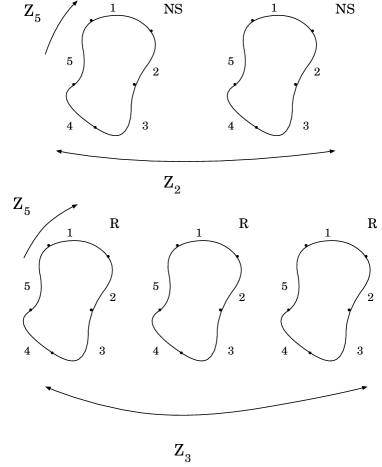
Figure 1: Same type of long strings are reshuffled in each irriduceble sets

In order to evaluate the partition function explicitly, we should decompose these elements into the “irreducible sets”. In the element of the centralizer group, $S_{N_{n}}$ can be decomposed further into its conjugacy class as,

$$[S_{N_{n}}]=(1)^{M_{n,1}}(2)^{M_{n,2}}\cdots,$$ (2.20)

$$\sum_{s_{n}>0}s_{n}M_{n,s_{n}}=N_{n}.$$ (2.21)

The “irreducible set” is the pair $h\in{\bf Z}_{n}^{\otimes s_{n}}$, $g\in{\bf Z}_{n}^{\otimes s_{n}}\times{\bf Z}_{s_{n}}$.

For the fermionic field, the action of the centralizer group is more complicated than the bosonic case. From the consistency condition $hg=gh$, the action of the centralizer group is the rotations and reshuffling of the long strings which have the same length and belong to the same fermionic sector, and appropriate ${\bf Z}_{2}$ action. In the next subsection, we will discuss the action of the centralizer group in more detail.

Thus we see how the conjugacy classes and its centralizers decompose into the irreducible sets. The full partition function is evaluated as the sum of the product of the partition function for the irreducible sets.

2.2 Partition function for closed string

2.2.1 Fermionic partition function for the irreducible set

To consider the partition ffunction of the superstring theory on $S^{N}{\bf R}^{8}$, we have to evaluate that of the complex fermionic fields. For the fermionic fields, the orbifold group is extended to $S_{N}\times{\bf Z}_{2}^{\otimes N}$.

The irreducible sets can be reduced to $nm$ complex fermionic free fields where $h$ and $g$ act as,

$$h = {\rm diag}(A_{0}{\cal T}_{n},\cdots,A_{m-1}{\cal T}_{n}),$$

$$g = {\rm diag}(B_{0}{\cal T}_{n}^{p_{0}},\cdots,B_{m-1}{\cal T}_{n}^{p_{m-1}})\cdot{\overline{\cal T}}_{m}\,\,,$$ (2.22)

where ${\cal T}_{n}$ and ${\overline{\cal T}}_{m}$ acts on $nm$ free fermionic fields $\Psi^{I,J}$ ($I=0,\cdots,n-1$ and $J=0,\cdots,m-1$) as,

$$({\cal T}_{n}\cdot\Psi)^{I,J} = \Psi^{I+1,J},$$

$$({\overline{\cal T}}_{m}\cdot\Psi)^{I,J} = \Psi^{I,J+1}.$$ (2.23)

$A_{J}$’s and $B_{J}$’s are $n\times n$ matrices $A_{J}={\rm diag}({\bf e}\!\left[\frac{\alpha_{0,J}}{2}\right],\cdots,{\bf e}\!\left[\frac{\alpha_{n-1,J}}{2}\right])$,
$B_{J}={\rm diag}({\bf e}\!\left[\frac{\beta_{0,J}}{2}\right],\cdots,{\bf e}\!\left[\frac{\beta_{n-1,J}}{2}\right])$ where $\alpha_{I,J}$ and $\beta_{I,J}$ takes their values in $0$ or $1$. The actions of $h$ and $g$ on $\Psi$ are written asas,

$$(h\cdot\Psi)^{I,J} = {\bf e}\!\left[\frac{\alpha_{I,J}}{2}\right]\Psi^{I+1,J},$$

$$(g\cdot\Psi)^{I,J} = {\bf e}\!\left[\frac{\beta_{I,J}}{2}\right]\Psi^{I+p_{J},J+1},$$ (2.24)

The consistency condition $hg=gh$ becomes nontrivial conditions for $\alpha$’s and $\beta$’s as,

$$\beta_{I,J}+\alpha_{I+P_{J},J+1}=\alpha_{I,J}+\beta_{I+1,J}.$$ (2.25)

Taking a sum of $I$ in the above relation, the condition for $\alpha_{J}\equiv\sum_{I=0}^{n-1}\alpha_{I,J}$ is

$$\alpha_{J}=\alpha_{J+1}.$$ (2.26)

Thus $\alpha_{J}$’s do not depend on $J$. This fact means that all long strings in the irreducible sets have same periodicity on space direction. So we define $\alpha\equiv\alpha_{J}$ where $\alpha$ is defined modulo 2.

By diagonalizing the action for $h$, we should introduce the basis for the fermionic field $\psi^{a,J}$ which is constructed from the discrete Fourier transformation of the fermionic field $\Psi^{I,J}$ as,

$$\psi^{a,J}\equiv\frac{1}{\sqrt{n}}\sum_{I=0}^{n-1}{\bf e}\!\left[-\frac{aI}{n}-\frac{\alpha I}{2n}+\sum_{K=0}^{I-1}\frac{\alpha_{K,J}}{2}\right]\Psi^{I,J},\quad a=0,\cdots n-1.$$ (2.27)

The mode expansion for $\psi^{a,J}$ is

$$\psi^{a,J}=i^{-1/2}\sum_{r\in{\bf Z}}\left(\psi_{r+\frac{a}{n}+\frac{\alpha}{2n}}^{a,J}e^{i(r+\frac{a}{n}+\frac{\alpha}{2n})w}+\tilde{\psi}_{r-\frac{a}{n}-\frac{\alpha}{2n}}^{a,J}e^{-i(r-\frac{a}{n}-\frac{\alpha}{2n})\bar{w}}\right),$$ (2.28)

where $w=\sigma^{1}+i\sigma^{0}$. Since the fermionic fields are complex fields, there are also conjugate fields $\bar{\Psi}^{I,J}$. The mode expansion for the conjugate field $\bar{\psi}^{a,J}$ is

$$\bar{\psi}^{a,J}=i^{-1/2}\sum_{r\in{\bf Z}}\left(\bar{\psi}_{r-\frac{a}{n}-\frac{\alpha}{2n}}^{a,J}e^{i(r-\frac{a}{n}-\frac{\alpha}{2n})w}+\tilde{\bar{\psi}}_{r+\frac{a}{n}+\frac{\alpha}{2n}}^{a,J}e^{-i(r+\frac{a}{n}+\frac{\alpha}{2n})\bar{w}}\right).$$ (2.29)

The commutation relations are

$$\{\psi_{r+\frac{a}{n}+\frac{\alpha}{2n}}^{a,J},\bar{\psi}_{s-\frac{b}{n}-\frac{\alpha}{2n}}^{b,L}\}=\delta_{J,L}\delta_{r+s,0}\delta_{a,b}.$$ (2.30)

The action of $g$ on this diagonalized basis $\psi^{a,J}$ becomes,

$$(g\cdot\psi)^{a,J}={\bf e}\!\left[\frac{\beta_{0,J}}{2}-\sum_{K=0}^{p_{J}-1}\frac{\alpha_{K,J+1}}{2}+\frac{ap_{J}}{n}+\frac{\alpha p_{J}}{2n}\right]\psi^{a,J+1}.$$ (2.31)

The eigenvalues for $g$ action are evaluated as,

$$\mu^{a,b}={\bf e}\!\left[\frac{\beta^{\{p\}}}{2m}+\frac{ap}{nm}+\frac{\alpha p}{2nm}+\frac{b}{m}\right],$$ (2.32)

$$p\equiv\sum_{J=0}^{m-1}p_{J},\quad\beta^{\{p\}}\equiv\sum_{J=0}^{m-1}\left(\beta_{0,J}-\sum_{K=0}^{p_{J}-1}\alpha_{K,J+1}\right),$$ (2.33)

$$a=0,\cdots,n-1,\quad b=0,\cdots,m-1.$$

The action of $g$ on diagonalized oscillator $\psi^{a,b}_{r+a/n+\alpha/2n}$ is written as,

$$(g\cdot\psi)^{a,b}_{r+a/n+\alpha/2n}=\mu^{a,b}\psi^{a,b}_{r+a/n+\alpha/2n}.$$ (2.34)

Using these diagonalized fields, the (chiral) oscillator part of the partition function can be evaluated as,

$$\prod_{a=0}^{n-1}\prod_{b=0}^{m-1}\prod_{r=1}^{\infty}\left(1-{\bf e}\!\left[\frac{\beta^{\{p\}}}{2m}+\frac{ap}{nm}+\frac{\alpha p}{2nm}+\frac{b}{m}\right]{\bf e}\!\left[(r-a/n-\alpha/2n)\tau\right]\right),$$ (2.35)

$$= \prod_{a=0}^{n-1}\prod_{r=1}^{\infty}\left(1-{\bf e}\!\left[\frac{\beta^{\{p\}}}{2}+\frac{ap}{n}+\frac{ap}{2n}\right]{\bf e}\!\left[(r-a/n-\alpha/2n)m\tau\right]\right),$$

$$= \prod_{a=0}^{n-1}\prod_{r=1}^{\infty}\left(1-{\bf e}\!\left[\frac{\beta^{\{p\}}}{2}\right]{\bf e}\!\left[-p(r-a/n-\alpha/2n)\right]{\bf e}\!\left[(r-a/n-\alpha/2n)m\tau\right]\right),$$

$$= \prod_{s\in{\bf N}-\alpha/2}\left(1-{\bf e}\!\left[\frac{\beta^{\{p\}}}{2}\right]{\bf e}\!\left[\Bigl{(}\frac{m\tau-p}{n}\Bigr{)}s\right]\right).$$

Thus the partition function for the $nm$ fermionic strings in the irreducible set are knitted together to give the partition function for the one long fermionic string on the torus with modified moduli parameter $\tau_{n,m,p}$,

$$\tau_{n,m,p}\equiv\frac{m\tau-p}{n}.$$ (2.36)

To evaluate the full partition function for the irreducible set, we need to add some important factors. At first, we consider the multiplicity of $\alpha_{J}$’s and $\beta_{J}$’s. If we sum over all $\alpha_{J}$’s and $\beta_{J}$’s, the value of $\alpha$ and $\beta^{\{p\}}$ can be taken freely. So under fixing $\alpha$ and $\beta^{\{p\}}$, the number of the multiplicity of $\alpha_{J}$’s and $\beta_{J}$’s is $2^{nm-1}$. Thus we have to add the factor as ($Z_{2}$ is the action of fermionic boundary condition),

$$\frac{2^{nm-1}}{|Z_{2}|^{nm}}=\frac{1}{2}.$$ (2.37)

And we replace $\beta^{\{p\}}$ to $\beta$.

Next we consider the zero-point energy. The zero-point energy for the fermionic field which has the fractional moding as ${\bf Z}-\theta$ is[23],

$$-\frac{1}{2}\omega^{\theta}\equiv-\frac{1}{2}\sum_{n=1}^{\infty}(n-\theta)=-\frac{1}{48}-\frac{1}{16}(2\theta-1)^{2}.$$ (2.38)

Therefore the zero-point energy of a (complex) fermionic string with length $n$ on $S^{N}\bf{R}^{2}$ is

$$\sum_{a=0}^{n-1}\left(-\frac{1}{2}\omega^{\theta=\frac{a}{n}+\frac{\alpha}{2n}}-\frac{1}{2}\omega^{\theta=1-\frac{a}{n}-\frac{\alpha}{2n}}\right),$$ (2.39)

$$= \sum_{a=0}^{n-1}\left(-\frac{1}{24}+\frac{1}{8}\Bigl{\{}2(\frac{a}{n}+\frac{\alpha}{2n})-1\Bigr{\}}^{2}\right),$$

$$= \frac{1}{12n}-\frac{\alpha}{4n}+\frac{\alpha^{2}}{8n}.$$

Thus the zero-point energy for the long string with length $n$ is $\frac{1}{n}$ of short string zero-point energy.

Here we consider the oscillator part of conjugate fermionic fields $\bar{\Psi}^{I,J}$. The calculation is the same as that of $\Psi^{I,J}$ . The result is

$$\prod_{s\in{\bf N}-(1-\alpha/2)}\left(1-{\bf e}\!\left[\frac{-\beta^{\{p\}}}{2}\right]{\bf e}\!\left[\Bigl{(}\frac{m\tau-p}{n}\Bigr{)}s\right]\right).$$ (2.40)

Finally we consider the various factors that comes from the vacuum. Since the vacuum for the $\psi^{a,b}_{r-a/n-\alpha/2n}$ ($0\leq a/n+\alpha/2n\leq 1/2$) has charge $\frac{1}{2}-\frac{a+\alpha/2}{n}$, the contribution from the ground state charge for the irreducible set is evaluated as,

$${\bf e}\Bigl{[}\frac{(\beta^{\{p\}}-1)(1-\alpha)}{8}-\frac{p}{8n}\left(\alpha^{2}-2\alpha\right)-\frac{(\tilde{\beta}^{\{p\}}-1)(1-\tilde{\alpha})}{8}+\frac{p}{8n}\left(\tilde{\alpha}^{2}-2\tilde{\alpha}\right)\Bigr{]}.$$ (2.41)

For the irreducible set of $nm$ strings, $m$ long string with length $n$ moving coherently. Its toggled vacuum is assigned to the toggled world-sheet as ordinary strings. So the fermion number of the vacuum and the space-time fermion number for the various sector is the same as that of ordinary string theory.

Gathering all these factors, the full (chiral) fermionic partition function for the irreducible set of $S^{N}{\bf R}^{8}$ is expressed as follows.[23, 24]

Type IIA,B

$$Z^{II}(n,m,\{p\}|\tau,\bar{\tau})=Z^{+}(\tau_{n,m,p})Z^{\pm}(\bar{\tau}_{n,m,p})^{*},$$ (2.42)

$$Z^{\pm}(\tau)=\frac{1}{2}[Z^{0}_{0}(\tau)^{4}-Z^{0}_{1}(\tau)^{4}-Z^{1}_{0}(\tau)^{4}\mp Z^{1}_{1}(\tau)^{4}],$$ (2.43)

$$Z^{a}_{b}(\tau)\equiv q^{(3a^{2}-1)/24}{\bf e}\!\left[ab/8\right]$$

$$\quad\quad\quad\quad\times\prod_{m=1}^{\infty}\Bigl{(}1-{\bf e}\!\left[b/2\right]q^{m-(1-a)/2}\Bigr{)}\Bigl{(}1-{\bf e}\!\left[-b/2\right]q^{m-(1+a)/2}\Bigr{)},$$ (2.44)

where $q\equiv{\bf e}\!\left[\tau\right]$.

Type 0A,B

$$Z^{0}(n,m,\{p\}|\tau,\bar{\tau})=\frac{1}{2}[|Z^{0}_{0}|^{N}+|Z^{0}_{1}|^{N}+|Z^{1}_{0}|^{N}+|Z^{1}_{1}|^{N}].$$ (2.45)

where $N=8$.

Thus we obtained the partition function for the irreducible set of the $S^{N}{\bf R}^{8}$.

2.2.2 Generating function of the partition function

As we obtained the partition function for the irreducible sets, we evaluate the partition function on $S^{N}{\bf R}^{8}$ by summing all products of irreducible sets. The combinatorial feature of the partition function for the irreducible set is same as that of bosonic case.[1]

The partition function for each conjugacy class (2.2) can be written as follows,

$$\chi_{h,g} = \prod_{n,s_{n}>0}(n^{s_{n}}Z(n,s_{n}))^{M_{n},s_{n}},$$ (2.46)

$$Z(n,m) = \frac{1}{n^{m}}\sum_{\{p\}}Z(n,m,\{p\}|\tau,\bar{\tau})=\frac{1}{n}\sum_{p}Z(n,m,p|\tau,\bar{\tau}).$$ (2.47)

Gathering all factors, the whole partition function is written as,

$$Z_{N}(\tau,\bar{\tau}) = \sum_{\scriptsize\begin{array}[]{c}N_{n},M_{n,m}\geq 1\\ \sum nN_{n}=N\\ \sum mM_{n,m}=N_{n}\end{array}}\prod_{n,m\geq 1}\frac{1}{M_{n,m}!}\left(\frac{1}{m}Z(n,m|\tau,\bar{\tau})\right)^{M_{n,m}}.$$ (2.51)

The generating function of the partition function can be evaluated as,

$$Z(\zeta|\tau,\bar{\tau}) \equiv \sum_{N=0}^{\infty}\zeta^{N}Z_{N}(\tau,\bar{\tau}),$$ (2.52)

$$= \exp\left(\sum_{N=1}^{\infty}\zeta^{N}{\cal V}_{N}\cdot Z_{1}(\tau,\bar{\tau})\right),$$

$${\cal V}_{N}\cdot f(\tau,\bar{\tau}) \equiv \frac{1}{N}\sum_{\scriptsize\begin{array}[]{c}a,d=1,\cdots,N\\ b=0,\cdots,d-1\\ ad=N\end{array}}f\left(\frac{a\tau+b}{d},\frac{a\bar{\tau}+b}{d}\right)$$ (2.56)

The operator ${\cal V}_{N}$ is called Hecke operator[25, 26] which maps a modular form to another one with the same weight.

In large $N$ limit, this partition function becomes as,

$$\sum_{m=1}^{\infty}\frac{1}{nm}\sum_{p=0}^{n-1}Z_{1}(\tau,\bar{\tau})\to\int\frac{d^{2}\tau}{{\rm Im}\tau}Z_{1}(\tau,\bar{\tau}).$$ (2.57)

Thus our partition function can be interpreted as the discretized version of the ordinary amplitude for the light-cone quantization. As we reproduced the integral of moduli in the continuum limit, we set the redundant variable $\tau$ to $\tau=i$.

3 Open Superstring on Symmetric Product

We will consider the open superstring theory on the symmetric product space. The nature of the second-quantized open string can be established by the evaluation of the partition function. Since the Hilbert space of the open string sector can be determined by specifying the boundary conditions, we have to calssify the boundary condition. The twisted sector in the open string theory on the abelian orbifold is well-known.[27, 28] Although the boundary condition for the abelian orbifold reduces to Neumann or Dirichlet condition, the boundary condition for the non-abelian orbifold has various sectors. The consistency condition for the bosonic boundary condition on the non-abelian orbifold is discussed in the previous work.[1] In this article, we generalize the previous results to fermionic case and then calculate the partition function for the permutation orbifold.

3.1 Open string Hilbert space

The Hilbert space for the open string is specified by the two boundary conditions. In this subsection, we concentrate on the fermionic fields. The fermionic action for the ordinary string is,

$$S=-\frac{i}{2\pi}\int_{0}^{\pi}d\sigma^{1}\int_{-\infty}^{\infty}d\sigma^{0}\Psi(\sigma^{0},\sigma^{1})\rho_{\alpha}\partial_{\alpha}\Psi(\sigma^{0},\sigma^{1}),$$ (3.1)

where $\rho_{\alpha}$ is two-dimensional Dirac matrix. The translation invariance of the action gives the boundary condition for the fermionic field,

$$\Psi_{L}(\sigma^{0},\sigma^{1}_{0})\pm f\Psi_{R}(\sigma^{0},\sigma^{1}_{0})=0,\quad f\in{\bf Z}_{2},$$ (3.2)

where $\sigma^{1}_{0}$ is the boundary value of $\sigma^{1}$. The sign $\pm$ in the boundary condition are referred as Neumann and Dirichlet condition. When the values of $f$ take different value at two boundary, this sector is called Neveu-Schwarz (NS) sector and when the values of $f$ take same value at two boundary, this sector is called Ramond (R) sector. Thus the Hilbert space of the open string is specified by the boundary conditions.

Next we will discuss the case that the target space is the orbifold $M/\Gamma$. At the fixed point of the action of the discrete group $\Gamma$, the boundary condition for the fermionic field is modified as,[29]

$$\Psi_{L}(\sigma^{0},\sigma^{1}_{0})\pm f\cdot\Psi_{R}(\sigma^{0},\sigma^{1}_{0})=0,\quad f\in\Gamma\times{\bf Z}_{2}.$$ (3.3)

We assume that the left- and right-mover have the same form of the boundary condition for the orbifold action and admit the asymmetry for the fermionic ${\bf Z}_{2}$ part,

$$f^{2}={\cal E},\quad{\cal E}\in\Gamma\times{\bf Z}_{2},$$ (3.4)

where ${\cal E}$ belongs to the identity element in $\Gamma$.

For the permutation orbifold, the boundary twist $f$ belongs to the conjugacy class as,

$$f\in\left[(1)^{N_{1}}(2)^{N_{2}}\right]\times{\bf Z}_{2}^{\otimes N},$$ (3.5)

where $N=N_{1}+2N_{2}$. The physical interpretation of this boundary twist is as follows. The boundary twist in the element of $(1)$ expresses the loose end of the string. In this article, we assign Neumann condition for this boundary condition to discuss the fundamental string. On the other hand, the boundary twist if the element of $(2)$ expresses the connection of two strings at this boundary. In this article, we assign Dirichlet condition for this boundary condition because two strings are connected smoothly.

Figure 2: Long open (closed) superstrings

The open string Hilbert space for the permutation orbifold can be specified by choosing the two boundary twists $f_{1}$, $f_{2}$ as above. For example, we illustrate the situation for a long open string (Figure 2 left),

$$f_{1} = \left[+{\cal T}_{1}\right]\otimes\left[{\rm diag}(-1,-1){\cal T}_{2}\right]\otimes\left[-{\cal T}_{1}\right],$$

$$f_{2} = \left[{\rm diag(-1,-1)}{\cal T}_{2}\right]\otimes\left[{\rm diag}(+1,+1){\cal T}_{2}\right].$$

Three NS open string bits and one R open string bit are connected and constitute a NS long open string. The situation for a long closed string is (Figure 2 right),

$$f_{1} = \left[{\rm diag}(+1,+1){\cal T}_{2}\right]\otimes\left[{\rm diag}(-1,-1){\cal T}_{2}\right],$$

$$f_{2} = \left[{\rm diag(-1,-1)}{\cal T}_{2}\right]\otimes\left[{\rm diag}(-1,+1){\cal T}_{2}\right].$$

Three NS open string bits and one R open string bit are connected and constitute a NS-$\widetilde{{\rm R}}$ long closed string. It is clear that we may realize the long open and closed string of the arbirary length by the pair of the boundary twists $(f_{1},f_{2})$.

3.2 Partition function for Annulus diagram

The partition function for the oriented open superstring is defined on the annulus diagram,

$${\rm Tr}_{{\cal H}_{f_{1},f_{2}}}(g{\bf e}\!\left[\tau L_{0}\right]).$$ (3.6)

Here and in the following sections, the moduli parameter $\tau$ for the annulus is pure imaginary. We will discuss the partition function of the fermionic field in this section to obtain the superstring partition function.

The boundary conditions for the fermionic field are written as,

$$\Psi_{L}(\sigma^{0},0) = f_{1}\cdot\Psi_{R}(\sigma^{0},0),$$

$$\Psi_{L}(\sigma^{0},\pi) = f_{2}\cdot\Psi_{R}(\sigma^{0},\pi).$$ (3.7)

To write the mode expansion for this field, a chiral field $\Psi$ should be introduced on the double cover of the annulus diagram (Figure 3).[27]

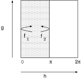
Figure 3: Double cover for annulus diagram

This chiral field has following periodicities,

$$\Psi(\sigma^{0},\sigma^{1}+2\pi)=h\cdot\Psi(\sigma^{0},\sigma^{1}),\quad\Psi(\sigma^{0}+2\pi,\sigma^{1})=g\cdot\Psi(\sigma^{0},\sigma^{1}).$$ (3.8)

For the consistency of the path integral, $h$ and $g$ must satisfy

$$hg=gh.$$ (3.9)

From the boundary condition at $\sigma^{1}=\pi$, the left- and right-moving fields are identified to this chiral field as,

$$\Psi_{L}(\sigma^{0},\sigma^{1})=\Psi(\sigma^{0},\sigma^{1}),\quad\Psi_{R}(\sigma^{0},\sigma^{1})=f_{2}\cdot\Psi(\sigma^{0},2\pi-\sigma^{1}),\quad 0\leq\sigma^{1}\leq\pi.$$ (3.10)

To satisfy the boundary condition at $\sigma^{1}=0$, $h$ and $f$’s must be related as,

$$h=f_{2}^{-1}\cdot f_{1}.$$ (3.11)

The consistency condition for the periodicity along the time direction and the boundary conditions is given as,

$$g\cdot f_{1}={\cal D}_{1}\cdot(f_{1}\cdot g),\quad g\cdot f_{2}={\cal D}_{2}\cdot(f_{2}\cdot g),$$ (3.12)

where ${\cal D}_{1}$, ${\cal D}_{2}$ are ${\bf Z}_{2}$ twists.

In the case of permutation group $\Gamma=S_{N}$, there are irreducible set of the twists $h,g,f_{1},f_{2}$. The irreducible set of the solution for the consistency conditions are classified into three types in bosonic case.[1]

• $I_{A}$ type solution:

  $$h = {\rm diag}(\overbrace{{\cal T}_{n},\cdots,{\cal T}_{n}}^{m}),$$

  $$g = {\rm diag}({\cal T}_{n}^{p_{0}},\cdots,{\cal T}_{n}^{p_{m-1}})\cdot{\overline{\cal T}}_{m},$$

  $$f_{1} = {\rm diag}({\cal T}_{n}^{q_{0}}{\cal S}_{n},\cdots,{\cal T}_{n}^{q_{m-1}}{\cal S}_{n}),$$

  $$f_{2} = {\rm diag}({\cal T}_{n}^{q_{0}+1}{\cal S}_{n},\cdots,{\cal T}_{n}^{q_{m-1}+1}{\cal S}_{n}),$$ (3.13)

  where $p_{J},q_{J}$ take their values in $0,1,\cdots,n-1$ (mod $n$) and $q_{J}$’s satisfy the condition,

  $$q_{J+1}-q_{J}\equiv 2p_{J}{(\mbox{mod}\,\,\,n)}.$$ (3.14)

• $II_{A}$ type solution:

  For even $m$, there is a solution which has the same form of $h$ and $g$ as $I_{A}$ case and $f_{i}$ takes the form as,

  $$f_{1} = {\rm diag}({\cal T}_{n}^{q_{0}}{\cal S}_{n},\cdots,{\cal T}_{n}^{q_{m-1}}{\cal S}_{n})\cdot({\overline{\cal T}}_{m/2})^{m/2},$$

  $$f_{2} = {\rm diag}({\cal T}_{n}^{q_{0}+1}{\cal S}_{n},\cdots,{\cal T}_{n}^{q_{m-1}+1}{\cal S}_{n})\cdot({\overline{\cal T}}_{m/2})^{m/2},$$ (3.15)

  where $p_{J}$ and $q_{J}$ satisfy the conditions,

  $$q_{J+1}-q_{J}\equiv p_{J}+p_{J+m/2},$$

  $$q_{J+m/2}\equiv q_{J},\quad{(\mbox{mod}\,\,\,n)}.$$ (3.16)

• $\widetilde{II}_{A}$ type solution:

  For even $m$, there is another solution which has the same form of $h$ and $f_{1}$,$f_{2}$ as $II_{A}$ case and $g$ takes the form as,

  $$g={\rm diag}({\cal T}_{n}^{p_{0}},\cdots,{\cal T}_{n}^{p_{m-1}})\cdot{\rm diag}({\overline{\cal T}}_{m/2},{\overline{\cal T}}_{m/2}),$$ (3.17)

  where $p_{J}$ and $q_{J}$ satisfy the conditions,

  $$q_{\tilde{J}}-q_{J}\equiv p_{J}+p_{J+m/2},$$

  $$q_{J+m/2}\equiv q_{J},\quad{(\mbox{mod}\,\,\,n)},$$ (3.18)

  where $\tilde{J}$ is defined as,

  $$\tilde{J}=\left\{\begin{array}[]{@{\,}ll}J^{\prime}&\mbox{($0\leq J\leq m/2-1$)}\\ J^{\prime}+m/2&\mbox{($m/2\leq J\leq m-1$)}\end{array}\right.$$ (3.21)

  $$J^{\prime}\equiv J+1\quad(\mbox{mod}\,\,\,m/2).$$

The solution for the fermionic fields are obtained by ${\bf Z}_{2}$ extension. In the following, we we will solve the consistency conditions for $I_{A}$, $II_{A}$ and $\widetilde{II}_{A}$.

3.2.1 Fermionic partition function for $I_{A}$

The periodicity and boundary condition for the $nm$ fermionic fields which corresponds to the $I_{A}$-type bosonic solution is,

$$h = {\rm diag}(A_{0}{\cal T}_{n},\cdots,A_{m-1}{\cal T}_{n}),$$

$$g = {\rm diag}(B_{0}{\cal T}_{n}^{p_{0}},\cdots,B_{m-1}{\cal T}_{n}^{p_{m-1}})\cdot{\overline{\cal T}}_{m},$$

$$f_{1} = {\rm diag}(F_{0}^{(1)}{\cal T}_{n}^{q_{0}}{\cal S}_{n},\cdots,F_{m-1}^{(1)}{\cal T}_{n}^{q_{m-1}}{\cal S}_{n}),$$

$$f_{2} = {\rm diag}(F_{0}^{(2)}{\cal T}_{n}^{q_{0}+1}{\cal S}_{n},\cdots,F_{m-1}^{(2)}{\cal T}_{n}^{q_{m-1}+1}{\cal S}_{n}),$$ (3.22)

where $A_{J}$, $B_{J}$ and $F_{J}^{(i)}$($i=1,2$) is the ${\bf Z}_{2}$ twists as,

$$A_{J} = {\rm diag}\left({\bf e}\!\left[\frac{\alpha_{0,J}}{2}\right],\cdots,{\bf e}\!\left[\frac{\alpha_{n-1,J}}{2}\right]\right),$$

$$B_{J} = {\rm diag}\left({\bf e}\!\left[\frac{\beta_{0,J}}{2}\right],\cdots,{\bf e}\!\left[\frac{\beta_{n-1,J}}{2}\right]\right),$$

$$F_{J}^{(i)} = {\rm diag}\left({\bf e}\!\left[\frac{\phi_{0,J}^{(i)}}{2}\right],\cdots,{\bf e}\!\left[\frac{\phi_{n-1,J}^{(i)}}{2}\right]\right),$$ (3.23)

$$J=0,\cdots,m-1,\quad i=1,2.$$

$\alpha_{I,J}$, $\beta_{I,J}$ and $\phi_{I,J}^{(i)}$ take value $0$ or $1$. From the fermionic consistency conditions (3.11), (3.9) and the left-right symmetry (3.4), $\alpha_{I,J}$, $\beta_{I,J}$ and $\phi_{I,J}^{(i)}$ are constrained as,

$$\alpha_{I,J}=\phi_{I,J}^{(1)}-\phi_{I+1,J}^{(2)},$$

$$\beta_{I,J}+\alpha_{I+p_{J},J+1}=\alpha_{I,J}+\beta_{I+1,J},$$

$$\phi_{I,J}^{(1)}+\phi_{n-1+q_{J}-I,J}^{(1)}=\epsilon_{I,J},$$

$$\phi_{I,J}^{(2)}+\phi_{n+q_{J}-I,J}^{(2)}=\epsilon_{I,J},$$ (3.24)

where these equations are defined mod $2$. $\epsilon_{I,J}$ is the matrix element of ${\cal E}$ in (3.4) which is defined as,

$${\cal E} = {\rm diag}\left(E_{0},\cdots,E_{m-1}\right)$$

$$E_{J} = {\rm diag}\left({\bf e}\!\left[\frac{\epsilon_{0,J}}{2}\right],\cdots,{\bf e}\!\left[\frac{\epsilon_{n-1,J}}{2}\right]\right),$$ (3.25)

where $\epsilon_{I,J}$’s take value 0 or 1. The constraint for $p_{J}$ and $q_{J}$ can be obtained from (3.12),

$$q_{J+1}-q_{J}\equiv 2p_{J},\quad(\mbox{mod}\,\,\,n).$$ (3.26)

If we sum up $J$, we obtain the following relation,

$$2p \equiv 0,\quad(\mbox{mod}\,\,\,n),$$ (3.27)

$$p \equiv \sum_{J=0}^{m-1}p_{J},$$

where $p$ is also defined mod $n$. From the condition (3.24), we obtain the following relation

$$\alpha_{J} = \alpha,\quad J=0,\cdots,m-1,$$ (3.28)

$$\alpha_{J} \equiv \sum_{I=0}^{n-1}\alpha_{I,J}.$$

Under these constraints, the action of $h$ and $g$ is diagonalized as torus case. The mode expansion for the diagonalized field $\psi^{a,J}$ with respect to $h$ is,

$$\psi^{a,J}_{L}(\sigma^{0},\sigma^{1}) = i^{-1/2}\sum_{r\in{\bf Z}}\psi^{a,J}_{r+\frac{a}{n}+\frac{\alpha_{J}}{2n}}{\rm exp}\left[i(r+\frac{a}{n}+\frac{\alpha_{J}}{2n})w\right],$$

$$\psi^{a,J}_{R}(\sigma^{0},\sigma^{1}) = (f_{2}\cdot\psi_{L})^{a,J}(\sigma^{0},\sigma^{1}),$$ (3.29)

$$= {\bf e}\!\left[-\frac{a+\alpha/2}{n}(n+q_{J})+\frac{\phi_{0,J}^{(2)}}{2}+\sum_{K=0}^{n+q_{J}-1}\frac{\alpha_{K,J}}{2}\right]$$

$$\times i^{-1/2}\sum_{r\in{\bf Z}}\bar{\psi}^{a,J}_{r-\frac{a}{n}-\frac{\alpha}{2n}}{\rm exp}\left[i(r-\frac{a}{n}-\frac{\alpha}{2})w\right].$$

The action of $g$ on the oscillators is evaluated as,

$$\left(g\cdot\psi_{r+\frac{a}{n}+\frac{\alpha}{2n}}\right)^{a,J}={\bf e}\!\left[\frac{\beta_{0,J}}{2}+\frac{(a+\alpha/2)p_{J}}{n}-\sum_{K=0}^{p_{J}-1}\frac{\alpha_{K,J+1}}{2}\right]\psi^{a,J+1}_{r+\frac{a}{n}+\frac{\alpha}{2n}}$$ (3.30)

Using the oscillators and the eigenvalues of $g$, we can evaluate the fermionic partition function for this condition. The calculation is the same as that of the torus case but the value of $p$ is restricted to $2p\equiv 0$ (mod $n$).

• Odd $n$ case:

  For odd $n$ case, only $p=0$ is admitted. The fermionic partition function for this case is,

  $$Z^{-}\left(\tau_{n,m,0}\right),$$ (3.31)

  $$\tau_{n,m,0}=\frac{m}{n}\tau.$$

  This can be interpreted as the partition function for the large annulus.

• Even $n$ case:

  For even $n$ case, $p=0$ and $p=n/2$ are admitted. The fermionic partition function for $p=0$ is same as above and the fermionic partition function for $p=n/2$ becomes,

  $$Z^{-}\left(\tau_{n,m,0}+1/2\right)$$ (3.32)

  This can be interpreted as the partition function for the large Möbius strip.

Thus from $I_{A}$ type solution, we obtain the annulus and Möbius strip amplitude for the long string.

3.2.2 Fermionic partition function for $II_{A}$

For even $m$, we have the solution which corresponds to the bosonic $II_{A}$-type. The solution has the same form as $I_{A}$ case for $h$ and $g$. The solution for $f_{1}$ and $f_{2}$ is,

$$f_{1} = {\rm diag}(F_{0}^{(1)}{\cal T}_{n}^{q_{0}}{\cal S}_{n},\cdots,F_{m-1}^{(2)}{\cal T}_{n}^{q_{m-1}}{\cal S}_{n})\cdot{\overline{\cal T}}_{m}^{m/2},$$

$$f_{2} = {{\rm diag}}(F_{0}^{(2)}{\cal T}_{n}^{q_{0}+1}{\cal S}_{n},\cdots,F_{m-1}^{(2)}{\cal T}_{n}^{q_{m-1}}{\cal S}_{n})\cdot{\overline{\cal T}}_{m}^{m/2}.$$ (3.33)

The constraints for $\alpha_{I,J}$, $\beta_{I,J}$ and $\phi_{I,J}^{(i)}$ which come from the fermionic consistency conditions (3.11) and (3.9) is same as that of $I_{A}$-type solution. The constraints which come from the left-right symmetry (3.4) is

$$\phi_{I,J}^{(1)}+\phi_{n-1+q_{J}-I,J+k}^{(1)} = \epsilon_{I,J},$$

$$\phi_{I,J}^{(2)}+\phi_{n+q_{J}-I,J+k}^{(2)} = \epsilon_{I,J},$$ (3.34)

where $k=m/2$. The constrints for $p_{J}$ and $q_{J}$ is,

$$q_{J+1}-q_{J} \equiv p_{J}+p_{J+m/2},\quad(\mbox{mod}\,\,\,n),$$

$$q_{J} = q_{J+k}.$$ (3.35)

Summing up $J$, we obtain the following relation,

$$\sum_{J=0}^{2k-1}p_{J}=0,$$ (3.36)

where we denote $k\equiv m/2$.

Under these constraints, we will evaluate the eigenvalue for $h$ and $g$. The mode expansion which satisfies this boundary condition can be obtained as $I_{A}$ case,

$$\psi^{a,J}_{L}(\sigma^{0},\sigma^{1}) = i^{-1/2}\sum_{r\in{\bf Z}}\psi^{a,J}_{r+\frac{a}{n}+\frac{\alpha_{J}}{2n}}{\rm exp}\left[i(r+\frac{a}{n}+\frac{\alpha_{J}}{2n})w\right],$$

$$\psi^{a,J}_{R}(\sigma^{0},\sigma^{1}) = {\bf e}\!\left[-\frac{a+\alpha_{J}/2}{n}(n+q_{J})+\frac{\phi_{0,J}^{(2)}}{2}+\sum_{K=0}^{n+q_{J}-1}\frac{\alpha_{K,J+k}}{2}\right]$$ (3.37)

$$\times i^{-1/2}\sum_{r\in{\bf Z}}\bar{\psi}^{a,J+k}_{r-\frac{a}{n}-\frac{\alpha_{J+k}}{2n}}{\rm exp}\left[i(r-\frac{a}{n}-\frac{\alpha_{J+k}}{2})w\right],$$

where we used the relation $\alpha_{J}=\alpha$ for all $J=0,\cdots,m-1$ as $I_{A}$ case. The action of $g$ is the same as $I_{A}$ case.

Thus the partition function can be calculated as the torus with $p=0$ as,

$$Z^{-}(2\tau_{n,k,0}).$$ (3.38)

This partition function can be interpreted as the Klein bottle partition function for the long string.

3.2.3 Fermionic partition function for $\widetilde{II}_{A}$

For even $m$, we have another solution which corresponds to the bosonic $\widetilde{II}_{A}$-type solution. This solution has same $h$, $f_{1}$ and $f_{2}$ as the $II_{A}$-type solution. The solution for $g$ is

$$g={\rm diag}(B_{0}{\cal T}_{n}^{p_{0}},\cdots,B_{m-1}{\cal T}_{n}^{p_{m-1}})\cdot{\rm diag}({\overline{\cal T}}_{m/2},{\overline{\cal T}}_{m/2}).$$ (3.39)

From the consistency condition, $p$’s and $q$’s should satisfy the constraints as,

$$q_{\tilde{J}}-q_{J}\equiv p_{J}+p_{J+m/2},\quad q_{J+m/2} = q_{J},$$ (3.40)

where the $\tilde{J}$ is defined as,

$$\tilde{J}=\left\{\begin{array}[]{@{\,}ll}J^{\prime}&\mbox{($0\leq J\leq m/2-1$)}\\ J^{\prime}+m/2&\mbox{($m/2\leq J\leq m-1$)}\end{array}\right.$$ (3.43)

$$J^{\prime}\equiv J+1\quad(\mbox{mod}\,\,\,m/2).$$

By the consistency condition (3.9), we have the constraint for $\alpha_{I,J}$ and $\beta_{I,J}$ as,

$$\alpha_{I,J}+\beta_{I+1,J}=\beta_{I,J}+\alpha_{I+p_{J},\tilde{J}}.$$ (3.44)

The other constraints are same as $II_{A}$ case.

The mode expansions for the fermionic fields are same as $II_{A}$ case (3.37). In $\widetilde{II}_{A}$ case, we should define

$$\alpha_{L} \equiv \alpha_{J},\quad J=0,1,\cdots,k-1,$$

$$\alpha_{R} \equiv \alpha_{J},\quad J=k,k+1,\cdots,m-1,$$ (3.45)

where we denote $k\equiv m/2$. $\alpha_{L}$ and $\alpha_{R}$ do not depend on $J$ by the constraint (3.44) and take independent value.

The eigenvalue of $g$ is evaluated independently for the diagonalized field $\Psi^{a,J}$ ($J=0,\cdots,k-1$) and $\Psi^{a,J}$ ($J=k,\cdots,m-1$).

From the consistency condition (3.12),

$$q_{\tilde{J}}-q_{J}\equiv p_{J+k}+p_{J},\quad(\mbox{mod}\,\,\,n),$$

$$q_{J}=q_{J+k}.$$ (3.46)

Therefore $p_{L}\equiv\sum_{J=0}^{k-1}p_{J}$ and $p_{R}\equiv\sum_{J=k}^{m-1}p_{J}$ are related as,

$$p_{L}=-p_{R}\equiv p\quad(\mbox{mod}\,\,\,n).$$ (3.47)

The oscillator part of the partition function for $\Psi^{I,J}$ is evaluated as,

$$\prod_{r\in{\bf N}-\alpha_{L}/2}\left(1-{\bf e}\!\left[\frac{\beta_{L}^{\{p\}}-1}{2}\right]{\bf e}\!\left[\frac{k\tau-p}{n}r\right]\right)\prod_{s\in{\bf N}-\alpha_{R}/2}\left(1-{\bf e}\!\left[\frac{\beta_{R}^{\{p\}}-1}{2}\right]{\bf e}\!\left[\frac{k\tau+p}{n}s\right]\right),$$

$$\beta_{L}^{\{p\}}\equiv\sum_{J=0}^{k-1}(\beta_{0,J}+\sum_{K=0}^{p_{J}-1}\alpha_{K,J+1}),\quad\beta_{R}^{\{p\}}\equiv\sum_{J=k}^{m-1}(\beta_{0,J}+\sum_{K=0}^{p_{J}-1}\alpha_{K,J+1}).$$ (3.48)

Gathering various factors, we obtain the partition function for $\widetilde{II}_{A}$-type solutiuon,

$$Z^{-}(\tau_{n,k,p})Z^{-}(\bar{\tau}_{n,k,p})^{*},$$ (3.49)

Thus we obtained the torus partition function for the long string.

3.3 Partition function for Möbius strip diagram

The partition function for the unoriented open superstring is defined as that of the Möbius strip,

$${\rm Tr}_{{\cal H}_{f_{1},f_{2}}}(\Omega g{\bf e}\!\left[\tau L_{0}^{{\rm open}}\right]),$$ (3.50)

where $\Omega$ is the orientation flip for the open string.

From the path-integral consistency condition for this partition function, the invariance of the Hilbert space under the action of $\Omega g$ is necessary. The action of $\Omega g$ on the left- and right-moving fermionic field is,

$$\Omega g\cdot\Psi_{L}(\sigma^{1}) = g\cdot\Psi_{R}(\pi-\sigma^{1}),$$

$$\Omega g\cdot\Psi_{R}(\sigma^{1}) = {\cal C}g\cdot\Psi_{L}(\pi-\sigma^{1}).$$ (3.51)

Since these fermionic fields satisfy the open string boundary condition (3.7), the boundary condition for $\Omega g$ acted fermionic field is,

$$\Omega g\cdot\Psi_{R}(0) = {\cal C}g\cdot\Psi_{L}(\pi),$$ (3.52)

$$= {\cal C}gf_{2}^{-1}\cdot\Psi_{R}(\pi),$$

$$= {\cal C}gf_{2}^{-1}g^{-1}\cdot\left(\Omega g\cdot\Psi_{R}(0)\right),$$

where we denoted the boundary condition at $\sigma^{1}=0$, the boundary condition at $\sigma^{1}=\pi$ can be evaluated as above. As the boundary condition must be invariant under the action of $\Omega g$ for the consistency of the Hilbert space, we need the constraint,

$$f_{1}={\cal C}gf_{2}^{-1}g^{-1},\quad f_{2}={\cal C}gf_{1}^{-1}g^{-1}.$$ (3.53)

The twist along the time direction can be obtained as,

$$h=f_{2}^{-1}f_{1}=gf_{1}g^{-1}{\cal C}^{-1}f_{1}.$$ (3.54)

If these $h$ and $g$ satisfy the consistency condition for the unoriented world sheet,

$$ghg^{-1}=h^{-1},$$ (3.55)

${\cal C}$, $f_{1}$, $f_{2}$, and $g$ should be constrained as,

$$gf_{1}^{2}g^{-1}={\cal C}f_{1}{\cal C}f_{1}.$$ (3.56)

In terms of the path integral on the Möbius strip diagram, the fermionic fields in the Hilbert space ${\cal H}_{f_{1},f_{2}}$ must satisfy the following conditions at $\sigma^{1}=0,\pi/2$,

$$\Psi_{R}(\sigma^{0},0) = f_{1}\cdot\Psi_{L}(\sigma^{0},0),$$

$$\Psi_{R}(\sigma^{0}+\pi,\pi/2) = {\cal C}g\cdot\Psi_{L}(\sigma^{0},\pi/2),$$

$$\Psi_{L}(\sigma^{0}+\pi,\pi/2) = g\cdot\Psi_{R}(\sigma^{0},\pi/2).$$ (3.57)

The boundary condition at $\sigma^{1}=\pi/2$ is the cross-cap condition. It is consistent if the following condition is satisfied,

$$[g,{\cal C}]=0.$$ (3.58)

In order to consider the mode expansion, we introduce the chiral field $\Psi$ on the double cover of the Möbius diagram (Figure 4).[27]

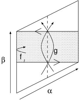
Figure 4: Double cover for Möbius strip diagram

The chiral field satisfies the following periodicity,

$$\Psi(\sigma^{0}+\pi,\sigma^{1}+\pi) = \alpha\cdot\Psi(\sigma^{0},\sigma^{1}),$$

$$\Psi(\sigma^{0}+2\pi,\sigma^{1}) = \beta\cdot\Psi(\sigma^{0},\sigma^{1}),\quad\alpha,\beta\in\Gamma\times{\bf Z}_{2}.$$ (3.59)

By the above boundary conditions, the chiral field $\Psi$ and the fields in ${\cal H}_{f_{1},f_{2}}$ can be identified as,

$$\Psi_{L}(\sigma^{0},\sigma^{1}) = \Psi(\sigma^{0},\sigma^{1}),$$

$$\Psi_{R}(\sigma^{0},\sigma^{1}) = g^{-1}\cdot\Psi(\sigma^{0}+\pi,\pi-\sigma^{1}).$$ (3.60)

The periodicities can be written by the boundary twists as,

$$\alpha=gf_{1},\quad\beta={\cal C}g^{2}.$$ (3.61)

The periodicity and the boundary condition along $\sigma^{1}=0$ implies,

$$[f_{1},\beta]=[f_{1},{\cal C}g^{2}]=0.$$ (3.62)

Thus we specfied the unoriented open string Hilbert space from the boundary conditions and obtained the consistent boundary conditions.

In the bosonic case[1], the solution of the periodicity and the boundary conditions for the irreducible set of the permutation group are calssified as $I_{M}$, $II_{M}$ and $\widetilde{II}_{M}$.

• $I_{M}$ type solution:

  $$h = {\rm diag}(\overbrace{{\cal T}_{n},\cdots,{\cal T}_{n}}^{m}),$$

  $$g = {\rm diag}({\cal T}_{n}^{p_{0}}{\cal S}_{n},\cdots,{\cal T}_{n}^{p_{m-1}}{\cal S}_{n})\cdot{\overline{\cal T}}_{m},$$

  $$f_{1} = {\rm diag}({\cal T}_{n}^{q_{0}}{\cal S}_{n},\cdots,{\cal T}_{n}^{q_{m-1}}{\cal S}_{n}),$$ (3.63)

  where $p_{J},q_{J}$ take their values in $0,1,\cdots,n-1$ (mod $n$) and $p_{J}$ and $q_{J}$ satisfy the condition,

  $$q_{J+1}+q_{J}\equiv 2p_{J}-1{(\mbox{mod}\,\,\,n)}.$$ (3.64)

• $II_{M}$ type solution:

  For even $m$, there is a solution which has the same form of $h$ and $g$ as $I_{M}$ case and $f_{1}$ takes the form as,

  $$f_{1}={\rm diag}({\cal T}_{n}^{q_{0}}{\cal S}_{n},\cdots,{\cal T}_{n}^{q_{m-1}}{\cal S}_{n})\cdot({\overline{\cal T}}_{m/2})^{m/2}$$ (3.65)

  where $p_{J}$ and $q_{J}$ satisfy the conditions,

  $$q_{J+1}+q_{J}\equiv p_{J}+p_{J+m/2}-1,$$

  $$q_{J+m/2}\equiv q_{J},\quad{(\mbox{mod}\,\,\,n)}.$$ (3.66)

• $\widetilde{II}_{M}$ type solution:

  For even $m$, there is another solution which has the same form of $h$ and $f_{1}$ as $II_{M}$ case and $g$ takes the form as,

  $$g={\rm diag}({\cal T}_{n}^{p_{0}}{\cal S}_{n},\cdots,{\cal T}_{n}^{p_{m-1}}{\cal S}_{n})\cdot{\rm diag}({\overline{\cal T}}_{m/2},{\overline{\cal T}}_{m/2}),$$ (3.67)

  where $p_{J}$ and $q_{J}$ satisfy the conditions,

  $$q_{\tilde{J}}+q_{J}\equiv p_{J}+p_{J+m/2}-1,$$

  $$q_{J+m/2}\equiv q_{J},\quad{(\mbox{mod}\,\,\,n)},$$ (3.68)

  where $\tilde{J}$ is defined as,

  $$\tilde{J}=\left\{\begin{array}[]{@{\,}ll}J^{\prime}&\mbox{($0\leq J\leq m/2-1$)}\\ J^{\prime}+m/2&\mbox{($m/2\leq J\leq m-1$)}\end{array}\right.$$ (3.71)

  $$J^{\prime}\equiv J+1\quad(\mbox{mod}\,\,\,m/2).$$

The solution for the fermionic boundary conditions can be obtained by ${\bf Z}_{2}$-extending the bosonic solution and then solving the consistency condition for the ${\bf Z}_{2}$-twists.

3.3.1 Fermionic partition function for $I_{M}$

The periodicity and the boundary condition for $nm$ fermionic fields which corresponds to the $I_{M}$-type bosonic solution is

$$h = {\rm diag}(A_{0}{\cal T}_{n},\cdots,A_{m-1}{\cal T}_{n}),$$

$$g = {\rm diag}(B_{0}{\cal T}_{n}^{p_{0}}{\cal S}_{n},\cdots,B_{m-1}{\cal T}_{n}^{p_{m-1}}{\cal S}_{n})\cdot{\overline{\cal T}}_{m},$$

$$f_{1} = {\rm diag}(F_{0}{\cal T}_{n}^{q_{0}}{\cal S}_{n},\cdots,F_{m-1}{\cal T}_{n}^{q_{m-1}}{\cal S}_{n}),$$

$${\cal C} = {\rm diag}(C_{0},\cdots,C_{m-1}),$$

$$C_{J} \equiv {\rm diag}\left({\bf e}\!\left[\frac{c_{0,J}}{2}\right],\cdots,{\bf e}\!\left[\frac{c_{n-1,J}}{2}\right]\right),\quad J=0,\cdots,m-1.$$ (3.72)

We will find the consistency condition for $\alpha$’s, $\beta$’s, $\phi$’s and $c$’s. From the consistency condition for the Möbius strip diagram (3.58),(3.54),(3.62),(3.56), we obtain the following relations,

$$c_{I,J}=c_{n-1-I+p_{J},J+1},$$

$$\alpha_{I,J}=\phi_{I,J}+\phi_{I+p_{J-1}-q_{J},J-1}-\beta_{I+p_{J-1}-q_{J},J-1}$$

$$\quad\quad\quad+\beta_{n-1+q_{J-1}+q_{J}-p_{J-1}-I,J-1}+c_{n-1-I+q_{J},J},$$

$$2p_{J-1}-q_{J-1}-q_{J}\equiv 1\quad{(\mbox{mod}\,\,\,n)},$$

$$\phi_{I,J}+\phi_{I+P_{J+1}-p_{J},J+2}-(c_{I,J}-c_{n-1+q_{J}-I,J})$$

$$\quad-(\beta_{I,J}-\beta_{n-1+q_{J}-I,J})+(\beta_{I+p_{J}-q_{J},J+1}-\beta_{n-1+p_{J}-I,J+1})=0,$$

$$\phi_{n-1+p_{J-1}-I,J-1}+\phi_{I+q_{J-1}-p_{J-1},J-1},$$

$$\quad=\phi_{I,J}+c_{I,J}+\phi_{n-1+q_{J}-I,J}+c_{n-1+q_{J}-I,J}.$$ (3.73)

If we sum up $I$ in the above constraints, we obtain the following relations,

$$\alpha_{J}=\phi_{J}-\phi_{J-1}+c_{J},\quad\phi_{J}=\phi_{J+2},\quad c_{J}=c_{J+1},$$ (3.74)

$$\alpha_{J}\equiv\sum_{I=0}^{n-1}\alpha_{I,J},\quad c_{J}\equiv\sum_{I=0}^{n-1}c_{I,J},\quad\phi_{J}\equiv\sum_{I=0}^{n-1}\phi_{I,J}.$$

Using these relations, we get

$$\alpha_{J}\equiv\alpha,\quad J=0,\cdots,m-1.$$ (3.75)

Under these constraints, the action of $\Omega g$ on the oscillator $\psi_{r+\frac{a}{n}+\frac{\alpha}{2n}}^{a,J}$ in the mode expansion (3.29) is evaluated as,

$$(\Omega g\cdot\psi)_{r+\frac{a}{n}+\frac{\alpha}{2n}}^{a,J}=$$

$${\bf e}\!\left[\frac{a+\alpha/2}{n}(p_{J}-q_{J})+\frac{1}{2}\left(\phi_{0,J}+\beta_{n-1+q_{J},J}-\sum_{K=0}^{p_{J}-q_{J}-1}\alpha_{K,J+1}\right)-\frac{a+\alpha/2}{2n}\right]$$

$$\times(-1)^{r}\psi_{r+\frac{a}{n}+\frac{\alpha}{2n}}^{a,J+1}.$$ (3.76)

The eigenvalue for $\Omega g$ is evaluated as torus case by diagonalizing $J$.

Thus the oscillator part of the partition function for $I_{M}$ case is calculated as,

$$\prod_{a=0}^{n-1}\prod_{b=0}^{m-1}Z_{a,b}=\prod_{r=1}^{\infty}\prod_{a=0}^{n-1}\left(1-(-1)^{mr}{\bf e}\!\left[\frac{\beta^{\{p,q\}}}{2}\right]{\bf e}\!\left[\frac{a+\alpha/2}{n}\cdot\frac{p}{2}\right]{\bf e}\!\left[m\tau(r-\frac{a}{n}-\frac{\alpha}{2n})\right]\right),$$

$$p\equiv\sum_{J=0}^{m-1}(2p_{J}-2q_{J}-1),\quad\beta^{\{p,q\}}\equiv\sum_{J=0}^{m-1}\left(\phi_{0,J}+\beta_{n-1+q_{J},J}-\sum_{K=0}^{p_{J}-q_{J}-1}\alpha_{K,J+1}\right).$$ (3.77)

The constraint (3.73) implies $p\equiv 0$ (mod $n$). However we need to evaluate it in mod $2n$ to get the accurate phase factor. So the partition function can be classified as follows.

• $n$:odd and $m$:odd

  In this case, only $p\equiv n$ (mod $2n$) can be admitted. Using the relation $(-1)^{ms}=(-1)^{s}=(-1)^{ns}$ and gathering all factors, we obtain the partition function,

  $$Z(n,m|\tau)=Z^{-}(\tau_{n,m,0}+\frac{1}{2}).$$ (3.78)

  In this case, we can interpret this result as the partition function for the large Möbius strip.

• $n$:odd and $m$:even

  In this case, only $p\equiv 0$ (mod $2n$) can be admitted. Using $(-1)^{ms}=1$ and gathering all factors, we obtain the partition function,

  $$Z(n,m|\tau)=Z^{-}(\tau_{n,m,0}).$$ (3.79)

  In this case, we can interpret this result as the partition function for the large annulus.

• $n$:even and $m$:even

  In this case, $p\equiv 0,n$ (mod $2n$) can be admitted. The partition function can be calculated as above.

  1. $p\equiv 0$ case

     If we use $(-1)^{ms}=1$, the partition function becomes,

     $$Z(n,m|\tau)=Z^{-}(\tau_{n,m,0}).$$ (3.80)

     Thus we obtained the partition function for the large annulus.

  2. $p\equiv n$ case

     If we use $(-1)^{ms}=1=(-1)^{ns}$, the partition function becomes,

     $$Z(n,m|\tau)=Z^{-}(\tau_{n,m,0}+1/2).$$ (3.81)

     Thus we obtained the partition function for the large Möbius strip.

3.3.2 Fermionic partition function for $II_{M}$

For even $m$, we have the solution which corresponds to the bosonic $II_{M}$-type solution. The solution has the same form as $I_{M}$ case for $h$ and $g$. The solution for $f_{1}$ is

$$f_{1}={\rm diag}(F_{0}{\cal T}_{n}^{q_{0}}{\cal S}_{n},\cdots,F_{m-1}{\cal T}_{n}^{q_{m-1}}{\cal S}_{n})\cdot{\overline{\cal T}}_{m}^{m/2}.$$ (3.82)

In this case, the consistency condition becomes,

$$\alpha_{I,J}=\phi_{I,J}+\phi_{I+p_{J+k-1}-q_{J},J+k-1}-\beta_{I+p_{J+k-1}-q_{J},J+k-1}$$

$$\quad\quad\quad+\beta_{n-1+q_{J+k-1}+q_{J}-p_{J+k-1}-I,J-1}+c_{n-1-I+q_{J},J+k},$$

$$p_{J-1}+p_{J+k-1}-q_{J+k-1}-q_{J}\equiv 1,\quad{(\mbox{mod}\,\,\,n)},$$

$$q_{J}=q_{J+k},$$

$$\phi_{I,J}+\phi_{I+P_{J+1}-p_{J},J+2}-(c_{I,J}-c_{n-1+q_{J}-I,J+k})$$

$$-(\beta_{I,J}-\beta_{n-1+q_{J}-I,J+k})+(\beta_{I+p_{J+k}-q_{J},J+k+1}-\beta_{n-1+p_{J}-I,J+1})=0,$$

$$\phi_{n-1+p_{J-1}-I,J-1}+\phi_{I+q_{J-1}-p_{J-1},J+k-1},$$

$$\quad=\phi_{I,J}+c_{I,J}+\phi_{n-1+q_{J}-I,J+k}+c_{n-1+q_{J}-I,J+k}.$$ (3.83)

where we denote $k=m/2$. The condition $c_{J}$ is same as $I_{M}$ case. If we sum up $I$ in the above constraints, we obtain the following relations,

$$\alpha_{J}\equiv\phi_{J}+\phi_{J+k-1}+\beta_{J-1}-\beta_{J+k-1}+c_{J+k},$$

$$\phi_{J}-\phi_{J+2}\equiv(\beta_{J}-\beta_{J+k})-(\beta_{J+k+1}-\beta_{J+1})+(c_{J}-c_{J+k}),$$

$$\beta_{J}\equiv\sum_{I=0}^{n-1}\beta_{I,J}.$$ (3.84)

Using these relations, we get the recursion relation,

$$\alpha_{J}\equiv\alpha_{J+k+1}.$$ (3.85)

For odd $k$ case, this recursion relation is solved as,

$$\alpha_{R}\equiv\alpha_{0}=\alpha_{2}\cdots\alpha_{2k-2},\quad\alpha_{L}\equiv\alpha_{1}=\alpha_{3}\cdots\alpha_{2k-1}.$$ (3.86)

For even $k$ case, this recursion relation is solved as,

$$\alpha\equiv\alpha_{J},\quad J=0,\cdots,m-1.$$ (3.87)

Under these constraints, the action of $\Omega g$ on the oscillator in (3.37) is evaluated as,

$$(\Omega g\cdot\psi)_{r+\frac{a}{n}+\frac{\alpha_{J}}{2n}}^{a,J}=$$

$${\bf e}\!\left[\frac{a+\alpha_{J}/2}{n}(p_{J+k}-q_{J})+\frac{1}{2}\left(\phi_{0,J}+\beta_{n-1+q_{J},J+k}-\sum_{K=0}^{p_{J+k}-q_{J}-1}\alpha_{K,J+k+1}\right)-\frac{a+\alpha_{J}/2}{2n}\right]$$

$$\times(-1)^{r}\psi_{r+\frac{a}{n}+\frac{\alpha_{J}}{2n}}^{a,J+k+1}.$$ (3.88)

Since the value of $\alpha_{J}$ depends on $k$, we classify the partition function as follows.

• $k$:even case

  In this case, $\alpha_{J}=\alpha$. By the constraint (3.83), we have only $p\equiv\sum_{J=0}^{m-1}(2p_{J+k}-2q_{J}-1)=0$. Thus the oscillator part of the partition function is evaluated as,

  $$\prod_{a=0}^{n-1}\prod_{b=0}^{m-1}Z_{a,b}=\prod_{r\in{\bf N}-\alpha/2}\left(1-{\bf e}\!\left[\frac{\beta^{\{p,q\}}}{2}\right]{\bf e}\!\left[\frac{2k\tau}{n}r\right]\right),$$

  $$\beta^{\{p,q\}}\equiv\sum_{J=0}^{m-1}\left(\phi_{0,J}+\beta_{n-1+q_{J},J+k}+\sum_{K=0}^{p_{J+k}-q_{J}-1}\alpha_{K,J+k+1}\right).$$ (3.89)

  Gathering all factors, we obtain the partition function for $II_{M}$ case,

  $$Z(n,m|\tau)=Z^{-}(2\tau_{n,k,0}).$$ (3.90)

  Identifying $\psi^{a,J}$ as the left-mover for $J$:odd and as the right-mover for $J$:even, we can interpret this partition function as that of large Klein bottle.

• $k$:odd case

  In this case, we can take independent value for $\alpha_{L}$ and $\alpha_{R}$. So the partition functions are evaluated for odd and even $J$ independently. Thus the oscillator part of the partition function is evaluated as,

  $$\prod_{a=0}^{n-1}\prod_{b=0}^{k-1}Z_{a,b}^{J:{\rm odd}}Z_{a,b}^{J:{\rm even}},$$ (3.91)

  $$= \prod_{r\in{\bf N}-\alpha_{L}/2}\left(1-{\bf e}\!\left[\frac{\beta^{\{p,q\}}_{L}}{2}\right]{\bf e}\!\left[\frac{k\tau-p}{n}r\right]\right)\prod_{r\in{\bf N}-\alpha_{R}/2}\left(1-{\bf e}\!\left[\frac{\beta^{\{p,q\}}_{R}}{2}\right]{\bf e}\!\left[\frac{k\tau+p}{n}r\right]\right),$$

  $$p\equiv\sum_{M=0}^{k-1}p_{2M+1+k}-\sum_{M=0}^{k-1}q_{2M+1}-k/2,$$

  $$\beta^{\{p,q\}}_{L}\equiv\sum_{J:{\rm odd}}\left(\phi_{0,J}+\beta_{n-1+q_{J},J+k}-\sum_{K=0}^{p_{J+k}-q_{J}-1}\alpha_{K,J+k+1}\right),$$

  $$\beta^{\{p,q\}}_{R}\equiv\sum_{J:{\rm even}}\left(\phi_{0,J}+\beta_{n-1+q_{J},J+k}-\sum_{K=0}^{p_{J+k}-q_{J}-1}\alpha_{K,J+k+1}\right).$$

  Gathering all factors, we obtain the partition function,

  $$Z(n,m,p|\tau)=Z^{-}(\tau_{n,k,p})Z^{-}(\bar{\tau}_{n,k,p})^{*}.$$ (3.92)

  This can be interpreted as the partition function for the large torus. However, $p$ takes half-odd value. So we call this diagram “twisted” torus.

3.3.3 Fermionic partition function for $\widetilde{II}_{M}$

For even $m$, we have another solution which corresponds to the bosonic $\widetilde{II_{M}}$-type solution. The solution has the same form as $II_{M}$ case for $h$ and $f_{1}$. The solution for $g$ is

$$g={\rm diag}(B_{0}{\cal T}_{n}^{p_{0}}{\cal S}_{n},\cdots,B_{m-1}{\cal T}_{n}^{p_{m-1}}{\cal S}_{n})\cdot{\rm diag}({\cal T}_{m/2},{\cal T}_{m}/2).$$ (3.93)

The consistency condition becomes as,

$$c_{I,J}=c_{n-1+p_{J}-I,\tilde{J}},$$

$$\alpha_{I,J}=\phi_{I,J}+\phi_{I+p_{\hat{J}+k}-q_{J},\hat{J}+k}-\beta_{I+p_{\hat{J}+k}-q_{J},\hat{J}+k}$$

$$\quad\quad\quad+\beta_{n-1+q_{\hat{J}+k}+q_{J}-p_{\hat{J}+k}-I,\hat{J}}+c_{n-1-I+q_{J},J+k},$$

$$p_{J}+p_{J+k}-q_{J+k}-q_{\tilde{J}}\equiv 1,\quad{(\mbox{mod}\,\,\,n)},$$

$$q_{J}=q_{J+k},$$

$$\phi_{I,J}+\phi_{I+P_{\tilde{J}}-p_{J},\tilde{\tilde{J}}}-(c_{I,J}-c_{n-1+q_{J}-I,J+k})$$

$$-(\beta_{I,J}-\beta_{n-1+q_{J}-I,J+k})+(\beta_{I+p_{J+k}-q_{J},\tilde{J}+k}-\beta_{n-1+p_{J}-I,\tilde{J}})=0,$$

$$\phi_{n-1+p_{\hat{J}}-I,\hat{J}}+\phi_{I+q_{\hat{J}}-p_{\hat{J}},\hat{J}+k},$$

$$\quad=\phi_{I,J}+c_{I,J}+\phi_{n-1+q_{J}-I,J+k}+c_{n-1+q_{J}-I,J+k},$$ (3.94)

where we denoted as $k=m/2$ and defined $\hat{J}$ as,

$$\hat{J}=\left\{\begin{array}[]{@{\,}ll}J^{\prime\prime}&\mbox{($0\leq J\leq m/2-1$)}\\ J^{\prime\prime}+m/2&\mbox{($m/2\leq J\leq m-1$)}\end{array}\right.$$ (3.97)

$$J^{\prime\prime}\equiv J-1\quad(\mbox{mod}\,\,\,m/2).$$

As $II_{M}$ case, we can find the following relations. For even $k$,

$$\alpha_{R} \equiv \alpha_{0}=\alpha_{k+1}=\alpha_{2}=\cdots=\alpha_{k},$$

$$\alpha_{L} \equiv \alpha_{1}=\alpha_{k+2}=\alpha_{3}=\cdots=\alpha_{k+1}.$$ (3.98)

For odd $k$,

$$\alpha\equiv\alpha_{J},\quad J=0,\cdots,m-1.$$ (3.99)

The action of $\Omega g$ on the oscillator $\psi^{a,J}_{r+a/n+\alpha/2n}$ is written as,

$$(\Omega g\cdot\psi)_{r+\frac{a}{n}+\frac{\alpha_{J}}{2n}}^{a,J}=$$

$${\bf e}\!\left[\frac{a+\alpha_{J}/2}{n}(p_{J+k}-q_{J})+\frac{1}{2}\left(\phi_{0,J}+\beta_{n-1+q_{J},J+k}-\sum_{K=0}^{p_{J+k}-q_{J}-1}\alpha_{K,\tilde{J}+k}\right)-\frac{a+\alpha_{J}/2}{2n}\right]$$

$$\times(-1)^{r}\psi_{r+\frac{a}{n}+\frac{\alpha_{J}}{2n}}^{a,\tilde{J}+k}.$$ (3.100)

Since the value of $\alpha_{J}$ depends on $k$, we classify the partition function as follows.

• $k$:odd case

  In this case, $\alpha\equiv\alpha_{J}$. From the constraint (3.3.3), only $p=0$ can be admitted. The partition function can be calculated as in even $k$ case of $II_{M}$. The result is,

  $$Z(n,m|\tau)=Z^{-}(2\tau_{n,k,0}).$$ (3.101)

  This can be interpreted as the partition function on the large Klein bottle.

• $k$:even case

  In this case, $\alpha_{L}$ and $\alpha_{R}$ can take independent values. The partition function can be calculated as in odd $k$ case of $II_{M}$. The oscillator part of the partition function can be written as,

  $$\prod_{a=0}^{n-1}\prod_{b=0}^{k-1}Z_{a,b}^{L}Z_{a,b}^{R} = \prod_{r\in{\bf N}-\alpha_{L}}\left(1-{\bf e}\!\left[\frac{\beta^{\{p,q\}}_{L}}{2}\right]{\bf e}\!\left[\frac{k\tau-p}{n}r\right]\right)$$

  $$\times\prod_{r\in{\bf N}-\alpha_{R}}\left(1-{\bf e}\!\left[\frac{\beta^{\{p,q\}}_{R}}{2}\right]{\bf e}\!\left[\frac{k\tau+p}{n}r\right]\right),$$

  $$p \equiv \sum_{M=0}^{k/2-1}(p_{2M}+p_{2M+k+1})-\sum_{M=0}^{k-1}q_{M}-k/2,$$ (3.102)

  where $\beta^{\{p,q\}}_{L}$ and $\beta^{\{p,q\}}_{R}$ can be defined as $II_{M}$ case. Gathering all factors we obtain the partition function for $\widetilde{II}_{M}$ as,

  $$Z(n,m,p|\tau)=Z^{-}(\tau_{n,k,p})Z^{-}(\bar{\tau}_{n,k,p})^{*}.$$ (3.103)

  This can be interpreted as the partition function for the large torus.

3.4 Partition function for Klein bottle diagram

The partition function for the unoriented closed superstring is defined as,

$${\rm Tr}_{{\cal H}_{h}}\left(\Omega g{\bf e}\!\left[\tau(L_{0}+\tilde{L}_{0})\right]\right),$$ (3.104)

where $\Omega$ is the orientation flip operator for the closed string. We will consider the consistent boundary condition for fermions.

From the path-integral consistency condition for this partition function, the invariance of the Hilbert space under the action of $\Omega g$ is necessary. The actions of $\Omega g$ on the fermionic fields in the Hilbert space ${\cal H}_{h}$ are written as,

$$\Omega g\cdot\Psi(\sigma^{1}) = g\cdot\tilde{\Psi}(2\pi-\sigma^{1}),$$

$$\Omega g\cdot\tilde{\Psi}(\sigma^{1}) = g\cdot\Psi(2\pi-\sigma^{1}).$$ (3.105)

The periodicity of the $\Omega g$ acted fermionic field is evaluated as,

$$\Omega g\cdot\Psi(\sigma^{1}+2\pi) = g\cdot\tilde{\Psi}(-\sigma^{1}),$$ (3.106)

$$= gh^{-1}\cdot\tilde{\Psi}(2\pi-\sigma^{1}),$$

$$= gh^{-1}g^{-1}\cdot\left(\Omega g\cdot\Psi(\sigma^{1}+2\pi)\right).$$

As the Hilbert space ${\cal H}_{h}$ must be invariant under the action of $\Omega g$, we obtain the following constraint,

$$h^{-1}=ghg^{-1}.$$ (3.107)

In terms of the path integral on the Klein bottle diagram, the fermionic fields in the Hilbert space ${\cal H}_{h}$ must satisfy the following conditions at $\sigma^{1}=0,\pi$,

$$\Psi_{R}(\sigma^{0}+\pi,0)={\cal C}f_{1}\Psi_{L}(\sigma^{0},0),\quad\Psi_{L}(\sigma^{0}+\pi,0)=f_{1}\Psi_{R}(\sigma^{0},0),$$ (3.108)

$$\Psi_{R}(\sigma^{0}+\pi,\pi)={\cal C}f_{2}\Psi_{L}(\sigma^{0},\pi),\quad\Psi_{L}(\sigma^{0}+\pi,\pi)=f_{2}\Psi_{R}(\sigma^{0},\pi).$$ (3.109)

Both of these conditions are cross-cap conditions. These conditions are consistent if the boundary twists satisty the following conditions,

$$h=f_{2}^{-1}f_{1},$$

$$[f_{1},{\cal C}]=[f_{2},{\cal C}]=0.$$ (3.110)

In order to consider the mode expansion, we introduce the chiral field $\Psi$ on the double cover of the Klein bottle diagram (Figure 5).[27]

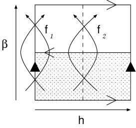
Figure 5: Double cover for Klein bottle diagram

This field has the following periodicities,

$$\Psi(\sigma^{0},\sigma^{1}+2\pi)=h\cdot\Psi(\sigma^{0},\sigma^{1}),\quad\Psi(\sigma^{0}+2\pi,\sigma^{1})=\beta\cdot\Psi(\sigma^{0},\sigma^{1}).$$ (3.111)

We identify these fields as,

$$\Psi_{L}(\sigma^{0},\sigma^{1})=\Psi(\sigma^{0},\sigma^{1}),\quad\Psi_{R}(\sigma^{0},\sigma^{1})={\cal C}f_{2}\Psi(\sigma^{0}-\pi,2\pi-\sigma^{1}).$$ (3.112)

The cross-cap conditions (3.108),(3.109), the twist $\beta$ must be written in terms of the boundary twists as,

$$\beta={\cal C}f_{1}^{2}={\cal C}f_{2}^{2}.$$ (3.113)

If we set $g=f_{1}$, two conditions (3.107) and (3.113) are identical.

In the bosonic case[1], the solution for $h$ and $g$ is obtained for the irreducible set of the permutation group,

$$h = {\rm diag}(\overbrace{{\cal T}_{n},\cdots,{\cal T}_{n}}^{m}),$$

$$g = {\rm diag}({\cal T}_{n}^{p_{0}}{\cal S}_{n},\cdots,{\cal T}_{n}^{p_{m-1}}{\cal S}_{n})\cdot{\overline{\cal T}}_{m}.$$ (3.114)

The solution for the fermions can be obtained by ${\bf Z}_{2}$ extention. We will find the consistency condition for ${\bf Z}_{2}$ twists and evaluate the partition function in the following.

3.4.1 Partition function for Klein bottle

The solution for $nm$ left-moving fermionic fields $\Psi^{I,J}$ on the Klein bottle diagram is

$$h = {\rm diag}(A_{0}{\cal T}_{n},\cdots,A_{m-1}{\cal T}_{n}),$$

$$g = {\rm diag}(B_{0}{\cal T}_{n}^{p_{0}}{\cal S}_{n},\cdots,B_{m-1}{\cal T}_{n}^{p_{m-1}}{\cal S}_{n})\cdot{\overline{\cal T}}_{m}.$$ (3.115)

The solution for $nm$ right-moving fermionic fields $\tilde{\Psi}^{I,J}$ is

$$h = {\rm diag}(\tilde{A}_{0}{\cal T}_{n},\cdots,\tilde{A}_{m-1}{\cal T}_{n}),$$

$$g = {\rm diag}(\tilde{B}_{0}{\cal T}_{n}^{p_{0}}{\cal S}_{n},\cdots,\tilde{B}_{m-1}{\cal T}_{n}^{p_{m-1}}{\cal S}_{n})\cdot{\overline{\cal T}}_{m},$$ (3.116)

where $\tilde{A}_{J}$ and $\tilde{B}_{J}$ are defined as,

$$\tilde{A}_{J} = {\rm diag}\left({\bf e}\!\left[\frac{\tilde{\alpha}_{0,J}}{2}\right],\cdots,{\bf e}\!\left[\frac{\tilde{\alpha}_{m-1,J}}{2}\right]\right),$$

$$\tilde{B}_{J} = {\rm diag}\left({\bf e}\!\left[\frac{\tilde{\beta}_{0,J}}{2}\right],\cdots,{\bf e}\!\left[\frac{\tilde{\beta}_{m-1,J}}{2}\right]\right).$$

By the consistency condition (3.107), the consistency condition for $\alpha$’s, $\beta$’s, $\tilde{\alpha}$’s and $\tilde{\beta}$’s become,

$$\alpha_{I,J}+\tilde{\alpha}_{n-2+p_{J}-I,J+1} = \beta_{I,J}-\beta_{I+1,J},$$

$$\tilde{\alpha}_{I,J}+\alpha_{n-2+p_{J}-I,J+1} = \tilde{\beta}_{I,J}-\tilde{\beta}_{I+1,J}.$$ (3.117)

Summing up $I$ in above relation, we obtain,

$$\alpha_{J}=-\tilde{\alpha}_{J+1},\quad\tilde{\alpha}_{J}=-\alpha_{J+1},$$

$$\tilde{\alpha}_{J}\equiv\sum_{I=0}^{n-1}\tilde{\alpha}_{I,J}.$$ (3.118)

For odd $m$ case, these relation can be solved as,

$$\alpha\equiv\alpha_{J}=-\tilde{\alpha}_{J},\quad J=0,\cdots,m-1.$$ (3.119)

For even $m$ case,

$$\alpha_{L}\equiv\alpha_{2J}=-\tilde{\alpha}_{2J+1},\quad\alpha_{R}\equiv\alpha_{2J+1}=-\tilde{\alpha}_{2J},\quad J=0,\cdots,m/2-1.$$ (3.120)

Under these constraints, we will evaluate the eigenvalue for $\Omega g$. $\Omega g$ acts on the fermionic field $\Psi,\tilde{\Psi}\in{\cal H}_{h}$ as,

$$(\Omega g\cdot\Psi)^{I,J}={\bf e}\!\left[\frac{\beta_{I,J}}{2}\right]\tilde{\Psi}^{n-1+p_{J}-I,J+1},\quad(\Omega g\cdot\tilde{\Psi})^{I,J}={\bf e}\!\left[\frac{\tilde{\beta}_{I,J}}{2}\right]\Psi^{n-1+p_{J}-I,J+1}.$$ (3.121)

Therefore the action of $\Omega g$ on the oscillator in the mode expansion (2.28) can be written as the Möbius strip case,

$$(\Omega g\cdot\psi)^{a,J}_{r+a/n+\alpha_{J}/2n} = {\bf e}\!\left[-\frac{a+\alpha_{J}/2}{n}(n-1+p_{J})+\frac{\beta_{0,J}}{2}-\sum_{K=0}^{n-2+p_{J}}\frac{\tilde{\alpha}_{K,J+1}}{2}\right]$$

$$\times\tilde{\psi}^{-a,J+1}_{r+a/n-\tilde{\alpha}_{J+1}/2n},$$

$$(\Omega g\cdot\tilde{\psi})^{-a,J}_{r+a/n-\tilde{\alpha}_{J}/2n} = {\bf e}\!\left[-\frac{a-\tilde{\alpha}_{J}/2}{n}(n-1+p_{J})+\frac{\tilde{\beta}_{0,J}}{2}-\sum_{K=0}^{n-2+p_{J}}\frac{\alpha_{K,J+1}}{2}\right]$$ (3.122)

$$\times\psi^{a,J+1}_{r+a/n+\alpha_{J+1}/2n}.$$

In order to evaluate the eigenvalue of $\Omega g$ on $\psi\tilde{\psi}$, we need to find a combination of left- and right-movers which is invariant up to scalar multiplication under the action of $\Omega g$. This combination must be taken between $\psi$’s in the same sector. So we consider even $m$ case and odd $m$ case case seperately in the following.

• Odd $m$ case:

  In this case, $\alpha_{J}=-\tilde{\alpha}_{J}\equiv\alpha$ holds. Therefore the liner combination can be defined as,

  $$d^{a}_{r+a/n+\alpha/2n} \equiv \sum_{J=0}^{m-1}D_{J}\psi^{a,J}_{r+a/n+\alpha/2n},$$

  $$\tilde{d}^{-a}_{r+a/n+\alpha/2n} \equiv (\Omega g\cdot d)^{a}_{r+a/n+\alpha/2n}.$$ (3.123)

  If one can find appropriate coefficients $D_{J}$ such that $d$’s satisfy,

  $$(\Omega g\cdot\tilde{d})^{a}_{r+a/n+\alpha/2n}=\lambda d^{a}_{r+a/n+\alpha/2n},$$ (3.124)

  $d^{a}_{r+a/n+\alpha/2n}\tilde{d}^{-a}_{r+a/n+\alpha/2n}$ becomes diagonal under the action of $\Omega g$.

  $$\Omega g\cdot(d^{a}_{r+a/n+\alpha/2n}\tilde{d}^{-a}_{r+a/n+\alpha/2n})=\lambda(d^{a}_{r+a/n+\alpha/2n}\tilde{d}^{-a}_{r+a/n+\alpha/2n}).$$ (3.125)

  The necessary recursion relation for $D_{J}$ is

  $$\lambda D_{J+2} = {\bf e}\Bigl{[}\frac{a+\alpha/2}{n}(p_{J+1}-p_{J})+\frac{\beta_{0,J}}{2}+\frac{\tilde{\beta}_{0,J+1}}{2}$$ (3.126)

  $$-\sum_{K=0}^{n+p_{J}-2}\frac{\tilde{\alpha}_{K,J+1}}{2}-\sum_{K=0}^{n+p_{J+1}-2}\frac{\alpha_{K,J+2}}{2}\Bigr{]}D_{J}.$$

  By using this recursion $m$ times and from the condition $D_{0}=D_{2m}$, the eigenvalue $\lambda_{b}$ for $\Omega g$ can be evaluated as,

  $$\lambda_{b} = {\bf e}\!\left[\frac{\beta^{\{p\}}}{2m}+\frac{b}{m}\right],$$ (3.127)

  $$\beta^{\{p\}} \equiv \sum_{l=0}^{m-1}\left(\beta_{0,J}+\tilde{\beta}_{0,J}-\sum_{K=0}^{n-2+p_{2l}}\tilde{\alpha}_{K,2l+1}-\sum_{K=0}^{n-2+p_{2l+1}}\alpha_{K,2l+2}\right).$$ (3.128)

  Thus we can evaluate the partition function. The oscillator part of the partition function is written as,

  $$\prod_{r\in{\bf N}-\alpha/2}\left(1-{\bf e}\!\left[\frac{\beta^{\{p\}}}{2}\right]{\bf e}\!\left[\frac{2m\tau}{n}r\right]\right).$$ (3.129)

  Gathering all factors we obtain the partition function for Klein bottle as,

  $$Z(n,m|\tau)=Z^{-}(2\tau_{n,m,0}).$$ (3.130)

  This can be interpreted as the partition function for the large Klein bottle.

• Even $m$ case:

  In this case, we have two different $\alpha$’s corresponding to even $J$ and odd $J$. So the eigenvalue for $\Omega g$ is evaluated independently as odd $m$ case, Therefore the partition function is evaluated as,

  $$\prod_{a=0}^{n-1}\prod_{b=0}^{m/2-1}Z^{J:{\rm even}}_{a,b}Z^{J:{\rm odd}}_{a,b}$$ (3.131)

  $$= \prod_{r\in{\bf N}-\alpha_{L}/2}\left(1-{\bf e}\!\left[\frac{\beta^{\{p\}}_{L}}{2}\right]{\bf e}\!\left[\frac{m\tau-p}{n}r\right]\right)\prod_{r\in{\bf N}-\alpha_{R}/2}\left(1-{\bf e}\!\left[\frac{\beta^{\{p\}}_{R}}{2}\right]{\bf e}\!\left[\frac{m\tau+p}{n}r\right]\right),$$

  $$\beta^{\{p\}}_{L}\equiv\sum_{l=0}^{m/2-1}\Biggl{(}\beta_{0,2l}+\beta_{0,2l+1}-\sum_{K=0}^{n-2+p_{m-2-2l}}\tilde{\alpha}_{K,m-1-2l}-\sum_{K=0}^{n-2+p_{m-1-2l}}\alpha_{K,m-2l}\Biggr{)},$$

  $$\beta_{R}^{\{p\}}\equiv\sum_{l=0}^{m/2-1}\Biggl{(}\beta_{0,2l+1}+\tilde{\beta}_{2l}-\sum_{K=0}^{n-2-p_{m-1-2l}}\tilde{\alpha}_{K,m-2l}-\sum_{K=0}^{n-2-p_{m-2-2l}}\alpha_{K,m-2l+1}\Biggr{)},$$

  $$p\equiv\sum_{l=0}^{m/2-1}p_{m-1-2l}-\sum_{l=0}^{m/2-1}p_{m-2l},$$

  Gathering all factors, we obtain the partition function for this case,

  $$Z(n,m,p|\tau)=Z^{-}(\tau_{n,m,p})Z^{-}(\bar{\tau}_{n,m,p})^{*}.$$ (3.132)

  This can be interpreted as the partition function for the large torus.

3.5 Generating function of Partition function

The partition functions for the irreducible sets are calculated for various topologies of the world-sheets. We proved that the interpretation for these partition functions can be made consistent with the bosonic open string case. Since the fermionic partition functions are classified in the same way as the bosonic case, we quote the table in the previous work[1] here.

Short string sector	$n$	$m$	Long string sector	Partition function
KB	$*$	odd	Klein Bottle	${\cal Z}^{KB}(\tau_{n,m,0})$
	$*$	even	Torus	${\cal Z}^{T}(\tau_{n,m,p},\bar{\tau}_{n,m,p})$
Annulus: $I_{A}$	odd	$*$	Annulus	${\cal Z}^{A}(\tau_{n,m,0})$
	even	$*$	Annulus+Möbius	${\cal Z}^{A}(\tau_{n,m,0})+{\cal Z}^{M}(\tau_{n,m,0})$
Annulus: $II_{A}$	$*$	$2\times*$	Klein Bottle	${\cal Z}^{KB}(\tau_{n,m/2,0})$
Annulus: $\widetilde{II}_{A}$	$*$	$2\times*$	Torus	${\cal Z}^{T}(\tau_{n,m/2,p},\bar{\tau}_{n,m/2,p})$
Möbius: $I_{M}$	odd	odd	Möbius	${\cal Z}^{M}(\tau_{n,m,0})$
	odd	even	Annulus	${\cal Z}^{A}(\tau_{n,m,0})$
	even	even	Annulus+Möbius	${\cal Z}^{A}(\tau_{n,m,0})+{\cal Z}^{M}(\tau_{n,m,0})$
	even	odd	—	0
Möbius: $II_{M}$	$*$	$2\times$odd	Torus	${\cal Z}^{T}(\tau_{n,m/2,p^{*}},\bar{\tau}_{n,m/2,p^{*}})$
	$*$	$2\times$even	Klein Bottle	${\cal Z}^{KB}(\tau_{n,m/2,0})$
Möbius: $\widetilde{II}_{M}$	$*$	$2\times$even	Torus	${\cal Z}^{T}(\tau_{n,m/2,p},\bar{\tau}_{n,m/2,p})$
	$*$	$2\times$odd	Klein Bottle	${\cal Z}^{KB}(\tau_{n,m/2,0})$

In this table, $p$ is an integer from $0$ to $n-1$ and $p^{*}$ is the half-odd integer from $0$ to $n$. The modular parameter is defined as $\tau_{n,m,p}\equiv(m\tau-p)/n$, where $\tau$ is pure imaginary.

The partition functions which appear in this table expressed as,

$${\cal Z}^{T}(\tau,\bar{\tau}) = ({\rm Im}\,\tau)^{-4}\frac{Z^{-}(\tau)}{\eta(\tau)^{8}}\cdot\left(\frac{Z^{-}(\bar{\tau})}{\eta(\bar{\tau})^{8}}\right)^{*},$$

$${\cal Z}^{A}(\tau) = N^{2}(2{\rm Im}\,\tau)^{-4}\frac{Z^{-}(\tau)}{\eta(\tau)^{8}},$$

$${\cal Z}^{MS}(\tau) = \eta N(2{\rm Im}\,\tau)^{-4}\frac{Z^{-}(\tau+1/2)}{\eta(\tau+1/2)^{8}},$$

$${\cal Z}^{KB}(\tau) = ({\rm Im}\,\tau)^{-4}\frac{Z^{-}(2\tau)}{\eta(2\tau)^{8}},$$ (3.133)

where $Z^{-}$ is defined as (2.43) and we denoted $N$ as the rank of the Chan-Paton group. When $\eta=1$, this group is $Sp(N)$ and when $\eta=-1$, this group is $SO(N)$.

By considering the combinatorial factors, the generating function of the partition function can be calculated as the closed string case. The proof for this is same as the bosonic open string case.[1] These functions can be also interpreted as the DLCQ partition functions. The result is as follows.

• Annulus:

  When the world-sheet topology is annulus, the partition function for the $S^{N}{\bf R}^{8}$ is defined as,

  $$Z_{N}^{A}(\tau)\equiv\frac{1}{N!}\sum_{h,g\in S_{N}}{\rm Tr}_{{\cal H}_{f_{1},f_{2}}}(g{\bf e}\!\left[\tau L_{0}\right]),$$ (3.134)

  with the constraints, $gf_{1}=D_{1}f_{1}g$, $gf_{2}={\cal D}_{2}f_{2}g$, $f_{1}^{2}=f_{2}^{2}={\cal E}$, $h=f_{2}^{-1}f_{1}$. The generating function for this partition function can be written as,

  $$\sum_{N=0}^{\infty}\zeta^{N}Z_{N}^{A}(\tau)$$ (3.135)

  $$= {\rm exp}\Biggl{(}\sum_{n,m=1}^{\infty}\frac{\zeta^{nm}}{m}{\cal Z}^{A}(\tau_{n,m,0})+\sum_{n,m=1}^{\infty}\frac{\zeta^{2nm}}{m}{\cal Z}^{MS}(\tau_{2n,m,0})$$

  $$+\sum_{n,m=1}^{\infty}\frac{\zeta^{2nm}}{2m}{\cal Z}^{KB}(\tau_{n,m,0})+\sum_{n,m=1}^{\infty}\frac{\zeta^{2nm}}{2nm}\sum_{p=0}^{n-1}{\cal Z}^{T}(\tau_{n,m,p},\bar{\tau}_{n,m,p})\Biggr{)}.$$

• Möbius strip:

  When the world-sheet topology is Möbius strip, the partition function for the $S^{N}{\bf R}^{8}$ is defined as,

  $$Z_{N}^{MS}(\tau)\equiv\frac{1}{N!}\sum_{h,g\in S_{N}}{\rm Tr}_{f_{1},f_{2}}(\Omega g{\bf e}\!\left[\tau L_{0}\right]),$$ (3.136)

  with the constraints, $f_{2}={\cal C}gf_{1}^{-1}g^{-1}$, $h=gf_{1}g^{-1}f$, $f_{1}^{2}={\cal E}$, $\left[{\cal C},g\right]=0$, $\left[{\cal C}g^{2},f_{1}\right]=0$. The generating function for this partition function can be written as,

  $$\sum_{N=0}^{\infty}\zeta^{N}Z_{N}^{MS}(\tau)$$ (3.137)

  $$= {\rm exp}\Biggl{(}\sum_{n,m=1}^{\infty}\frac{\zeta^{2nm}}{2m}{\cal Z}^{A}(\tau_{n,2m,0})$$

  $$+\sum_{n,m=1}^{\infty}\frac{\zeta^{(2n-1)m}}{m}{\cal Z}^{MS}(\tau_{2n-1,m,0})+\sum_{n,m=1}^{\infty}\frac{\zeta^{2nm}}{2m}{\cal Z}^{KB}(\tau_{n,m,0})$$

  $$+\sum_{n,m=1}^{\infty}\frac{\zeta^{2nm}}{2nm}\sum_{p=0}^{n-1}{\cal Z}^{T}(\tau_{n,m,p+n/2},\bar{\tau}_{n,m,p+n/2})\Biggr{)}.$$

• Klein bottle:

  When the world-sheet topology is Klein bottle, the partition function for the $S^{N}{\bf R}^{8}$ is defined as,

  $$Z_{N}^{MS}(\tau)\equiv\frac{1}{N!}\sum_{h,g\in S_{N}}{\rm Tr}_{h}(\Omega g{\bf e}\!\left[\tau L_{0}\right]),$$ (3.138)

  with a constraint $hg=gh^{-1}$. The generating function for this partition function can be written as,

  $$\sum_{N=0}^{\infty}\zeta^{N}Z_{N}^{KB}(\tau)$$ (3.139)

  $$= {\rm exp}\Biggl{(}\sum_{n,m=1}^{\infty}\frac{\zeta^{n(2m-1)}}{2m-1}{\cal Z}^{KB}(\tau_{n,2m-1,0})$$

  $$+\sum_{n,m=1}^{\infty}\frac{\zeta^{2nm}}{2nm}\sum_{p=0}^{n-1}{\cal Z}^{T}(\tau_{n,2m,p},\bar{\tau}_{n,2m,p})\Biggr{)}.$$

4 Boundary State for Fermionic Fields

In the previous section, we considered the open string on the permutation orbifold in the open string sector. In this section, we will construct the boundary state and see how the change of the world-sheet topology occurs. Here we concentrate on the case of $S^{N}{\bf R}^{1}$, since the generalization to $S^{N}{\bf R}^{8}$ is clear.

4.1 Boundary state for the irreducible sets

In terms of the closed string sector, we will consider the irreducible combination of the twist $g$ along the space direction and the boundary twist $f$. The closed string Hilbert space is specfied by the twist along the space direction. As discussed in section 2, we can decompose the Hilbert space ${\cal H}_{g}$ into that of the conjugacy class and from the condition $fg={\cal D}gf$, the boundary twist belongs to its centralizer group. Thus the irreducible combination of $(g,f)$ can be written as,

$$g={\rm diag}(A_{0}{\overline{\cal T}}_{{\overline{n}}},\cdots,A_{{\overline{m}}-1}{\overline{\cal T}}_{{\overline{n}}}),\quad f={\rm diag}(F_{0}{\overline{\cal T}}_{{\overline{n}}}^{{\overline{p}}_{0}},\cdots,F_{{\overline{m}}-1}{\overline{\cal T}}_{{\overline{n}}}^{{\overline{p}}_{m-1}})\cdot{\cal T}_{{\overline{m}}}.$$ (4.1)

For this irreducible combination of the twists, further constraint (3.4) must be imposed. This constraint needs the value of ${\overline{m}}$ to be $1$ or $2$. As a result, we can classify the irreducible sets into three types.

• ${\overline{m}}=1$, ${\overline{n}}$:odd case.

  In this case, the boundary twist $f$ can be written as $f=F_{0}{\overline{\cal T}}_{0}^{{\overline{p}}_{0}}$. The condition $f^{2}={\cal E}$ imposes the condition,

  $$2{\overline{p}}_{0}\equiv 0,\quad{(\mbox{mod}\,\,\,{\overline{n}})}.$$ (4.2)

  For odd ${\overline{m}}$ case, we have only one solution ${\overline{p}}_{0}\equiv 0$ (mod ${\overline{n}}$).

• ${\overline{m}}=1$, ${\overline{n}}$:even case.

  In this case, the boundary twist $f$ is same as above case. But there are two solutions for (4.2) as ${\overline{p}}_{0}\equiv 0$ (mod ${\overline{n}}$) and ${\overline{p}}_{0}\equiv{\overline{n}}/2$ (mod ${\overline{n}}$).

• ${\overline{m}}=2$ case.

  In this case, the boundary twist $f$ is written as $f={\rm diag}(F_{0}{\overline{\cal T}}_{{\overline{n}}},F_{1}{\overline{\cal T}}_{{\overline{n}}})\cdot{\cal T}_{2}$. The condition $f^{2}={\cal E}$ imposes the condition,

  $${\overline{p}}_{0}+{\overline{p}}_{1}\equiv 0,\quad{(\mbox{mod}\,\,\,{\overline{n}})}.$$ (4.3)

We will construct the boundary states corresponding to these boundary twists. Though we imposed the condition $fg={\cal D}gf$ in the open string setor, we impose the condition $fg=gf$ here and the non-commuting condition is imposed on another boundary.

(i)Boundary states for the long string:

In this case, the combination of twists is $(g,f)=(A{\overline{\cal T}}_{{\overline{n}}},F)$. The consistency condition $fg=gf$ implies,

$$\phi\equiv\phi_{{\overline{I}}},\quad f={\bf e}\!\left[\frac{\phi}{2}\right]\cdot{\bf 1}_{{\overline{n}}}.$$ (4.4)

If we use the mode expansion for the closed string (2.28), the boundary state can be written as,

$${|\,B:A{\overline{\cal T}}_{{\overline{n}}},F\rangle\!\rangle}=\exp\left(-i{\bf e}\!\left[\frac{\phi}{2}\right]\sum_{r=1}^{\infty}\sum_{a=0}^{{\overline{n}}-1}\psi^{(a)}_{-r+a/{\overline{n}}+\alpha/2{\overline{n}}}\tilde{\psi}^{({\overline{n}}-a)}_{-r+a/{\overline{n}}+\alpha/2{\overline{n}}}\right)|0\rangle_{{\overline{n}}},$$ (4.5)

where we denote $\alpha=\sum_{{\overline{I}}=0}^{{\overline{n}}-1}\alpha_{{\overline{I}}}.$

We introduce the long string oscillator of length ${\overline{n}}$ as,

$$\Psi_{{\overline{n}}r+a+\alpha/2}\equiv\psi^{(a)}_{r+a/{\overline{n}}+\alpha/2{\overline{n}}},\quad\tilde{\Psi}_{{\overline{n}}r+a+\alpha/2}\equiv\tilde{\psi}^{({\overline{n}}-a)}_{r+a/{\overline{n}}+\alpha/2{\overline{n}}}.$$ (4.6)

These oscillators satisfy the commutation relation $\{\Psi_{r},\Psi_{s}\}=\delta_{r+s,0}$. The commutation relation with Hamiltonian is modified to $[L_{0},\Psi_{r}]=-\frac{r}{{\overline{n}}}\Psi_{r}$. In terms of these variables, the boundary state can be rewritten as,

$$|B\rangle_{{\overline{n}}}\equiv\exp\left(-i{\bf e}\!\left[\frac{\phi}{2}\right]\sum_{r\in{\bf N}-\alpha/2}\Psi_{-r}\tilde{\Psi}_{-r}\right)|0\rangle_{{\overline{n}}}.$$ (4.7)

This boundary state can be interpreted as the boundary state for the long string.

(ii)Cross-cap states for the long string:

If ${\overline{n}}$ is even, there is a combination of twists $(g,f)=(A{\overline{\cal T}}_{{\overline{n}}},F{\overline{\cal T}}_{{\overline{n}}}^{{\overline{n}}/2})$. The consistency condition $fg=gf$ implies,

$$\phi_{{\overline{I}}}-\phi_{{\overline{I}}+1}=\alpha_{{\overline{I}}}-\alpha_{{\overline{I}}+{\overline{l}}},$$ (4.8)

where we denoted as ${\overline{l}}\equiv{\overline{n}}/2$. Under this relation, the action of $f$ on the diagonalized field $\psi^{(a)}$ becomes,

$$f\cdot\psi^{(a)} = {\bf e}\!\left[\frac{\beta}{2}\right](-1)^{a+\alpha/2}\psi^{(a)},$$ (4.9)

$$\beta \equiv \phi_{0}-\sum_{{\overline{K}}=0}^{{\overline{I}}-1}\alpha_{{\overline{K}}}.$$ (4.10)

In deriving above action, we used the relation,

$$\phi_{{\overline{I}}}-\sum_{{\overline{K}}=0}^{{\overline{I}}+{\overline{l}}-1}\alpha_{{\overline{K}}}+\sum_{{\overline{K}}=0}^{{\overline{I}}-1}\alpha_{{\overline{K}}}=\phi_{0}-\sum_{{\overline{K}}=0}^{{\overline{l}}-1}\alpha_{{\overline{K}}},$$

which is derived from the relation (4.8).

The boundary state for this twist can be written as,

$${|\,B:A{\overline{\cal T}}_{{\overline{n}}},F{\overline{\cal T}}_{{\overline{n}}}^{{\overline{n}}/2}\rangle\!\rangle}\equiv|C\rangle_{{\overline{n}}},$$ (4.11)

$$= \exp\left(-i{\bf e}\!\left[\frac{\beta}{2}\right]\sum_{r=1}^{\infty}\sum_{a=0}^{{\overline{n}}-1}(-1)^{a+\alpha/2}\psi^{(a)}_{-r+a/{\overline{n}}+\alpha/2{\overline{n}}}\tilde{\psi}^{({\overline{n}}-a)}_{-r+a/{\overline{n}}+\alpha/2{\overline{n}}}\right)|0\rangle_{{\overline{n}}},$$

$$= \exp\left(-i{\bf e}\!\left[\frac{\beta}{2}\right]\sum_{r\in{\bf N}-\alpha/2}(-1)^{r}\Psi_{-r}\tilde{\Psi}_{-r}\right)|0\rangle_{{\overline{n}}}.$$

This boundary state can be intepreted as the cross-cap state for the long string. This is the origin of the topology change from the oriented world-sheet to the unoriented one.

(iii)Joint state:

In this case, ${\overline{m}}=2$. and the combination of the twists is,

$$g=\left(\begin{array}[]{cc}A_{0}{\overline{\cal T}}_{{\overline{n}}}&0\\ 0&A_{1}{\overline{\cal T}}_{{\overline{n}}}\end{array}\right),\quad f=\left(\begin{array}[]{cc}0&F_{0}{\overline{\cal T}}_{{\overline{n}}}^{{\overline{p}}_{0}}\\ F_{1}{\overline{\cal T}}_{{\overline{n}}}^{{\overline{p}}_{1}}&0\end{array}\right).$$ (4.12)

The consistency condition $fg=gf$ implies,

$$\phi_{{\overline{I}},{\overline{J}}}-\phi_{{\overline{I}}+1,{\overline{J}}}=\alpha_{{\overline{I}},{\overline{J}}}-\alpha_{{\overline{I}}+{\overline{p}}_{{\overline{J}}},{\overline{J}}+1},$$ (4.13)

$${\overline{I}}=0,\cdots,{\overline{n}}-1,\quad{\overline{J}}=0,1.$$

Summing up ${\overline{I}}$, we obtain $\alpha\equiv\alpha_{{\overline{J}}}$.

Under this relation, the acion of $f$ on the diagonalid field $\psi^{(a,{\overline{J}})}$ can be written as,

$$f\cdot\psi^{(a,{\overline{J}})} = {\bf e}\!\left[\frac{\beta^{{\overline{p}}}}{2}+\frac{(a+\alpha/2){\overline{p}}_{{\overline{J}}}}{{\overline{n}}}\right]\psi^{(a,{\overline{J}}+1)},$$ (4.14)

$$\beta^{{\overline{p}}}_{{\overline{J}}} \equiv \phi_{0,{\overline{J}}}-\sum_{{\overline{K}}=0}^{{\overline{p}}_{{\overline{J}}}-1}\alpha_{{\overline{K}},{\overline{J}}+1}.$$ (4.15)

In deriving above action, we used the relation,

$$\phi_{{\overline{I}},{\overline{J}}}-\sum_{{\overline{K}}=0}^{{\overline{I}}+{\overline{p}}_{{\overline{J}}}-1}\alpha_{{\overline{K}},{\overline{J}}+1}+\sum_{{\overline{K}}=0}^{{\overline{I}}-1}\alpha_{{\overline{K}},{\overline{J}}}=\phi_{0,{\overline{J}}}-\sum_{{\overline{K}}=0}^{{\overline{p}}_{{\overline{J}}}-1}\alpha_{{\overline{K}},{\overline{J}}+1},$$

which is derived from the relation (4.13).

The boundary state for this twist can be written as,

$${|\,B:g,f\rangle\!\rangle}\equiv|J(12),{\overline{p}}\rangle_{{\overline{n}}},$$ (4.16)

$$= \exp\Biggl{(}i{\bf e}\!\left[\frac{\beta^{{\overline{p}}}_{0}}{2}\right]\sum_{r=1}^{\infty}\sum_{a=0}^{{\overline{n}}-1}{\bf e}\!\left[\frac{(a+\alpha/2){\overline{p}}}{{\overline{n}}}\right]\psi^{(a,1)}_{-r+a/{\overline{n}}+\alpha/2{\overline{n}}}\tilde{\psi}^{({\overline{n}}-a,2)}_{-r+a/{\overline{n}}+\alpha/2{\overline{n}}}$$

$$+i{\bf e}\!\left[\frac{\beta^{{\overline{p}}}_{1}}{2}\right]\sum_{r=1}^{\infty}\sum_{a=0}^{{\overline{n}}-1}{\bf e}\!\left[\frac{-(a+\alpha/2){\overline{p}}}{{\overline{n}}}\right]\psi^{(a,2)}_{-r+a/{\overline{n}}+\alpha/2{\overline{n}}}\tilde{\psi}^{({\overline{n}}-a,1)}_{-r+a/{\overline{n}}+\alpha/2{\overline{n}}}\Biggr{)}|0\rangle_{{\overline{n}}},$$

$$= \exp\Biggl{(}i{\bf e}\!\left[\frac{\beta^{{\overline{p}}}_{0}}{2}\right]\sum_{r\in{\bf N}-\alpha/2}{\bf e}\!\left[\frac{r{\overline{p}}}{{\overline{n}}}\right]\Psi^{(1)}_{-r}\tilde{\Psi}^{(2)}_{-r}$$

$$+i{\bf e}\!\left[\frac{\beta^{{\overline{p}}}_{1}}{2}\right]\sum_{r\in{\bf N}-\alpha/2}{\bf e}\!\left[-\frac{r{\overline{p}}}{{\overline{n}}}\right]\Psi^{(2)}_{-r}\tilde{\Psi}^{(1)}_{-r}\Biggr{)}|0\rangle_{{\overline{n}}},$$

where we denoted ${\overline{p}}\equiv{\overline{p}}_{0}=-{\overline{p}}_{1}$ and $\Psi^{({\overline{J}})}$ (${\overline{J}}$=1,2) is the oscillator for two long stings. This boundary state represents the interconnection of two long strings at the boundary. So we call this state as “Joint state”.

4.2 Cross-cap state for the irreducible set

As considered in the open string analysis, the cross-cap state satisfies $g=f^{2}{\cal C}$. The irreducible combination of the twists can be found from (4.1). The cross-cap condition impose the value of ${\overline{m}}$ to be $1$ or $2$. The boundary twists are classified as follows.

• ${\overline{m}}=1$ case.

  In this case, the boundary twists $f$ can be written as $f=F_{0}{\overline{\cal T}}_{{\overline{n}}}^{{\overline{p}}_{0}}$. The cross-cap condition $g=f^{2}{\cal C}$ imposes the following condition,

  $$2{\overline{p}}_{0}\equiv 1,\quad{(\mbox{mod}\,\,\,{\overline{n}})}.$$ (4.17)

  For odd ${\overline{n}}$ case, we have one solution ${\overline{p}}_{0}=({\overline{n}}-1)/2$. For even ${\overline{n}}$ case, we have no solution for above condition.

• ${\overline{m}}=2$ case.

  In this case, the boundary twist $f$ is written as $f={\rm diag}(F_{0}{\overline{\cal T}}_{{\overline{n}}},F_{1}{\overline{\cal T}}_{{\overline{n}}})\cdot{\cal T}_{2}$. The cross-cap condition $g=f^{2}{\cal C}$ imposes the following condition,

  $${\overline{p}}_{0}+{\overline{p}}_{1}\equiv 1,\quad{(\mbox{mod}\,\,\,{\overline{n}})}.$$ (4.18)

  We will construct the cross-cap states corresponding to these boundary twists.

(i)Cross-cap state for long string:

When ${\overline{m}}=1$, there is a combination of twists $(g,f)=(A{\overline{\cal T}}_{{\overline{n}}},F{\overline{\cal T}}_{{\overline{n}}}^{({\overline{n}}+1)/2})$ for odd ${\overline{n}}$. The constraint $[f,{\cal C}]=0$ and $[f,g]=0$ implies ${\cal C}={\rm diag}\left({\bf e}\!\left[\frac{c}{2}\right],\cdots,{\bf e}\!\left[\frac{c}{2}\right]\right)$.

From the constraint $g=f^{2}{\cal C}$, we obtain the condition as,

$$\alpha_{{\overline{I}}}=c+\phi_{{\overline{I}}}+\phi_{{\overline{I}}+({\overline{n}}+1)/2}.$$ (4.19)

The action of $f$ on the diagonalized field $\psi^{(a)}$ is

$$(f\cdot\psi)^{(a)}={\bf e}\!\left[\frac{a+\alpha/2}{{\overline{n}}}\cdot\frac{{\overline{n}}+1}{2}+\frac{({\overline{n}}+1)c}{4}+\frac{\phi}{2}\right]\psi^{(a)}.$$

The cross-cap condition is written as,

$$\left(\psi^{(a)}(\sigma^{0},\sigma^{1}+\pi)+if\cdot\tilde{\psi}^{({\overline{n}}-a)}(\sigma^{0},\sigma^{1})\right){|\,C:g,f\rangle\!\rangle}=0.$$ (4.20)

This condition is solved as,

$${|\,C:g,f\rangle\!\rangle} = \exp\Biggl{(}-i{\bf e}\!\left[\frac{\phi}{2}+\frac{({\overline{n}}+1)c}{4}\right]\sum_{s=1}^{\infty}\sum_{a=0}^{{\overline{n}}-1}$$ (4.21)

$$\times{\bf e}\!\left[\frac{s-a-\alpha/2}{2}\right]\psi^{(a)}_{-s+a/{\overline{n}}+\alpha/2{\overline{n}}}\tilde{\psi}^{({\overline{n}}-a)}_{-s+a/{\overline{n}}+\alpha/2{\overline{n}}}\Biggr{)}|0\rangle_{{\overline{n}}},$$

$$= \exp\left(-i{\bf e}\!\left[\frac{\phi}{2}+\frac{({\overline{n}}+1)c}{4}\right]\sum_{r\in{\bf N}-\alpha/2}(-1)^{r}\Psi_{-r}\tilde{\Psi}_{r}\right)|0\rangle_{{\overline{n}}}.$$

This can be interpreted as the cross-cap state for the long string.

(ii)Joint state:

For ${\overline{m}}=2$, we have the twists as,

$$g=\left(\begin{array}[]{cc}A_{0}{\overline{\cal T}}_{{\overline{n}}}&0\\ 0&A_{1}{\overline{\cal T}}_{{\overline{n}}}\end{array}\right),\quad f=\left(\begin{array}[]{cc}0&F_{0}{\overline{\cal T}}_{{\overline{n}}}^{{\overline{p}}_{0}}\\ F_{1}{\overline{\cal T}}_{{\overline{n}}}^{{\overline{p}}_{1}}&0\end{array}\right).$$ (4.22)

The condition $[f,{\cal C}]=0$ and $[g,f]=0$ implies ${\cal C}={\rm diag}(C,C)$, $C={\rm diag}({\bf e}\!\left[\frac{c}{2}\right],\cdots,{\bf e}\!\left[\frac{c}{2}\right])$.

From the constraint $g=f^{2}{\cal C}$, we obtain the condition as,

$$\alpha_{{\overline{I}},{\overline{J}}}=c+\phi_{{\overline{I}},{\overline{J}}}+\phi_{{\overline{I}}+{\overline{p}}_{{\overline{J}}},{\overline{J}}+1}.$$ (4.23)

Summing up ${\overline{I}}$, we obtain the relation $\alpha\equiv\alpha_{{\overline{J}}}$.

The action of $f$ on the diagonalized field $\psi^{(a,{\overline{J}})}$ is written as,

$$(f\cdot\psi)^{(a,{\overline{J}})} = {\bf e}\!\left[\frac{(a+\alpha/2)}{{\overline{n}}}+\frac{\beta^{{\overline{p}}}_{{\overline{J}}}}{2}\right]\psi^{(a,{\overline{J}}+1)},$$ (4.24)

$$\beta^{{\overline{p}}}_{{\overline{J}}} \equiv \phi_{0,{\overline{J}}}-\sum_{{\overline{K}}=0}^{{\overline{p}}_{{\overline{J}}}-1}\alpha_{{\overline{K}},{\overline{J}}+1}.$$ (4.25)

The cross-cap condition (4.20) is solved as,

$${|\,C:g,f\rangle\!\rangle}$$ (4.26)

$$= \exp\Biggl{(}i{\bf e}\!\left[\frac{\beta^{{\overline{p}}}_{0}}{2}\right]\sum_{s=1}^{\infty}\sum_{a=0}^{{\overline{n}}-1}(-1)^{-s+a/{\overline{n}}+\alpha/2{\overline{n}}}{\bf e}\!\left[(\frac{a}{{\overline{n}}}+\frac{\alpha}{2{\overline{n}}}){\overline{p}}\right]\psi^{(a,0)}_{-s+a/{\overline{n}}+\alpha/2{\overline{n}}}\tilde{\psi}^{(a,1)}_{-s+a/{\overline{n}}+\alpha/2{\overline{n}}}$$

$$+i{\bf e}\!\left[\frac{\beta^{{\overline{p}}}_{1}}{2}\right]\sum_{s=1}^{\infty}\sum_{a=0}^{{\overline{n}}-1}(-1)^{-s+a/{\overline{n}}+\alpha/2{\overline{n}}}{\bf e}\!\left[-(\frac{a}{{\overline{n}}}+\frac{\alpha}{2{\overline{n}}})({\overline{p}}+1)\right]\psi^{(a,1)}_{-s+a/{\overline{n}}+\alpha/2{\overline{n}}}\tilde{\psi}^{(a,0)}_{-s+a/{\overline{n}}+\alpha/2{\overline{n}}}\Biggr{)}|0\rangle_{{\overline{n}}},$$

$$= \exp\Biggl{(}i{\bf e}\!\left[\frac{\beta^{{\overline{p}}}_{0}}{2}\right]\sum_{s=1}^{\infty}\sum_{a=0}^{{\overline{n}}-1}(-1)^{-s}{\bf e}\!\left[(\frac{a}{{\overline{n}}}+\frac{\alpha}{2{\overline{n}}})({\overline{p}}+1/2)\right]\Psi^{(a,1)}_{-{\overline{n}}s+a+\alpha/2}\tilde{\Psi}^{(a,2)}_{-{\overline{n}}s+a+\alpha/2}$$

$$+i{\bf e}\!\left[\frac{\beta^{{\overline{p}}}_{1}}{2}\right]\sum_{s=1}^{\infty}\sum_{a=0}^{{\overline{n}}-1}(-1)^{-s}{\bf e}\!\left[-(\frac{a}{{\overline{n}}}+\frac{\alpha}{2{\overline{n}}})({\overline{p}}+1/2)\right]\Psi^{(a,1)}_{-{\overline{n}}s+a+\alpha/2}\tilde{\Psi}^{(a,2)}_{-{\overline{n}}s+a+\alpha/2}\Biggr{)}|0\rangle_{{\overline{n}}}.$$

Two short strings are connedted at this boundary in curious way. The factor ${\overline{p}}+1/2$ is the origin of the “half-twist” in the large torus amplitude.

4.3 Inner product between boundary states

In order to reproduce the open string amplitudes which we calculated in the previous section, we will consider the inner products between the boundary states. If the irriducibility condition for the periodicity and boundary twist is loosened, the open string partition functions for the irreducible sets can be realized. So we use the following general twists for the boundary conditions,

$$f_{1}={\rm diag}(F^{(1)}_{0}{\overline{\cal T}}_{{\overline{n}}}^{{\overline{p}}^{(1)}_{0}},\cdots,F^{(1)}_{{\overline{m}}-1}{\overline{\cal T}}_{{\overline{n}}}^{{\overline{p}}^{(1)}_{{\overline{m}}-1}})\cdot{\cal T}_{{\overline{m}}}^{{\overline{q}}_{1}}{\cal S}_{{\overline{m}}},$$

$$f_{2}={\rm diag}(F^{(2)}_{0}{\overline{\cal T}}_{{\overline{n}}}^{{\overline{p}}^{(2)}_{0}},\cdots,F^{(2)}_{{\overline{m}}-1}{\overline{\cal T}}_{{\overline{n}}}^{{\overline{p}}^{(2)}_{{\overline{m}}-1}})\cdot{\cal T}_{{\overline{m}}}^{{\overline{q}}_{2}}{\cal S}_{{\overline{m}}},$$ (4.27)

where these twists satisfy the condition $f_{i}^{2}={\cal E}$.

For the consistency of the amplitude, the condition $[h,g]=0$ must be satisfied. This condition gives the following constraint for $\alpha$ and $\phi^{(i)}$,

$$\alpha_{{\overline{I}},{\overline{J}}}-\alpha_{{\overline{I}}+{\overline{p}}^{(1)}_{{\overline{J}}}+{\overline{p}}^{(2)}_{{\overline{m}}-1-{\overline{J}}+{\overline{q}}_{1}},{\overline{J}}{\overline{q}}_{2}-{\overline{q}}_{1}}$$ (4.28)

$$= \phi^{(1)}_{{\overline{I}},{\overline{J}}}-\phi^{(1)}_{{\overline{I}}+1,{\overline{J}}}+\phi^{(2)}_{{\overline{I}}+{\overline{p}}^{(1)}_{{\overline{J}}},{\overline{m}}-1-{\overline{J}}+{\overline{q}}_{1}}-\phi^{(2)}_{{\overline{I}}+{\overline{p}}^{(1)}_{{\overline{J}}}+1,{\overline{m}}-1-{\overline{J}}+{\overline{q}}_{2}},$$

where we defined $h\equiv f_{2}f_{1}$. On the other hand, the condition $f_{i}^{2}={\cal E}$ gives the following constraint for $p_{{\overline{J}}}$ and $q_{{\overline{J}}}$ as,

$${\overline{p}}^{(i)}_{{\overline{J}}}+{\overline{p}}^{(i)}_{{\overline{m}}-1-{\overline{J}}+{\overline{q}}_{i}}\equiv 0\quad{(\mbox{mod}\,\,\,{\overline{n}})}.$$ (4.29)

To classify the amplitudes, we need to interpret the boundary condition physically. If there are string bits which is invariant under the boundary twist (4.27), the long string has the loose ends. The condition which the long string has the loose ends is,

$${\overline{l}}\equiv{\overline{m}}-1-{\overline{l}}+{\overline{q}}_{i}\quad{(\mbox{mod}\,\,\,{\overline{n}})}.$$ (4.30)

From the solution for this condition, we can classify the boundary twists into two types.

• Long open string boundary:

  If the boundary twists $f_{1}$ and $f_{2}$ admit two loose ends which satisfy the condition (4.30), this sector expresses the long open string. The condition for this case is that ${\overline{m}}$ is even and ${\overline{q}}_{1}-{\overline{q}}_{2}$ is odd or ${\overline{m}}$ is odd. So we set ${\overline{q}}_{1}=1$ and ${\overline{q}}_{2}=0$ as the representative.

  Before evaluating the eigenvalue of $h=f_{2}f_{1}$, the constraint (4.28) implies $\alpha\equiv\alpha_{{\overline{J}}}$. So the eigenvalue for $f_{2}f_{1}$ can be calculated as before,

  $$\mu_{a,b} = {\bf e}\!\left[\frac{(a+\alpha/2){\overline{p}}}{{\overline{n}}{\overline{m}}}+\frac{\beta^{\{{\overline{p}}^{(1)},{\overline{p}}^{(2)}\}}}{2{\overline{m}}}+\frac{b}{{\overline{m}}}\right],$$

  $${\overline{p}} \equiv \sum_{{\overline{J}}=0}^{{\overline{m}}-1}({\overline{p}}^{(1)}_{{\overline{J}}}+{\overline{p}}^{(2)}_{{\overline{J}}}),$$

  $$\beta^{\{{\overline{p}}^{(1)},{\overline{p}}^{(2)}\}} \equiv \sum_{{\overline{J}}=0}^{{\overline{m}}-1}\left(\phi^{(1)}_{0,{\overline{J}}}+\phi^{(2)}_{{\overline{p}}^{(1)}_{{\overline{J}}},{\overline{m}}-{\overline{J}}}-\sum_{{\overline{K}}=0}^{{\overline{p}}^{(1)}+{\overline{p}}^{(2)}_{{\overline{m}}-{\overline{J}}-1}-1}\alpha_{{\overline{K}},{\overline{J}}-1}\right).$$ (4.31)

  Because of (4.29), ${\overline{p}}$ depends only on the value at the loose ends ${\overline{p}}={\overline{p}}^{(1)}_{{\overline{l}}}+{\overline{p}}^{(2)}_{{\overline{l}}^{\prime}}$. For annulus and Klein bottle, we have ${\overline{p}}=0$ (mod ${\overline{n}}$). For Möbius strip, we have ${\overline{p}}={\overline{n}}/2$ (mod ${\overline{n}}$).

  In the explicit evaluation, we use the following formulae,

  $$\langle 0|e^{-if_{2}^{I,J}\psi_{I}\tilde{\psi}_{J}q}e^{-if_{1}^{K,L}\psi_{K}^{\dagger}\tilde{\psi}_{L}^{\dagger}}|0\rangle=\prod_{a}(1+\mu_{a}q),$$ (4.32)

  where oscillators satisfy the commutation relations $\{\psi_{I},\psi_{J}^{\dagger}\}=\{\tilde{\psi}_{I},\tilde{\psi}_{J}^{\dagger}\}=\delta_{I,J}$ and $\mu_{a}$ is the eigenvalue for $f_{2}f_{1}$.

  Thus the oscillator contributions of annulus and Klein bottle amplitudes are evaluated as,

  $${\langle\!\langle B:g,f_{2}\,|}q^{L_{0}+\tilde{L}_{0}}{|\,B:g,f_{1}\rangle\!\rangle}$$ (4.33)

  $$= \prod_{s=1}^{\infty}\prod_{a=0}^{{\overline{n}}-1}\prod_{b=0}^{{\overline{m}}-1}\left(1+{\bf e}\!\left[\frac{\beta^{\{{\overline{p}}^{(1)},{\overline{p}}^{(2)}\}}}{2{\overline{m}}}\right]{\bf e}\!\left[\frac{b}{{\overline{m}}}\right]q^{2(s-a/{\overline{n}}-\alpha/2{\overline{n}})}\right),$$

  $$= \prod_{r\in{\bf N}-\alpha/2}\left(1-{\bf e}\!\left[\frac{\beta^{\{{\overline{p}}^{(1)},{\overline{p}}^{(2)}\}}+{\overline{m}}}{2}\right]q^{2{\overline{m}}r/{\overline{n}}}\right).$$

  For Möbius strip, the oscillator contribution is written as,

  $${\langle\!\langle B:g,f_{2}\,|}q^{L_{0}+\tilde{L}_{0}}{|\,B:g,f_{1}\rangle\!\rangle}$$ (4.34)

  $$= \prod_{s=1}^{\infty}\prod_{a=0}^{{\overline{n}}-1}\prod_{b=0}^{{\overline{m}}-1}\left(1+{\bf e}\!\left[\frac{\beta^{\{{\overline{p}}^{(1)},{\overline{p}}^{(2)}\}}}{2{\overline{m}}}\right]{\bf e}\!\left[\frac{b}{{\overline{m}}}+\frac{a+\alpha/2}{2{\overline{m}}}\right]q^{2(s-a/{\overline{n}}-\alpha/2{\overline{n}})}\right),$$

  $$= \prod_{r\in{\bf N}-\alpha/2}\left(1-(-1)^{r}{\bf e}\!\left[\frac{\beta^{\{{\overline{p}}^{(1)},{\overline{p}}^{(2)}\}}+{\overline{m}}}{2}\right]q^{2{\overline{m}}r/{\overline{n}}}\right).$$

  Thus we have reproduced the annulus, Möbius strip and Klein bottle amplitudes for the long string from the inner products of the boundary states.

• Long closed string boundary:

  If the boundary twists $f_{1}$ and $f_{2}$ admit no loose end, this sector expresses the long closed string. In order not to have any solutions for the condition (4.30), the necessary condition is that ${\overline{m}}$ is even and both ${\overline{q}}_{1}$ and ${\overline{q}}_{2}$ is even. So we set ${\overline{m}}$ is even and ${\overline{q}}_{1}=2$ and ${\overline{q}}_{2}=0$ as the representative.

  From the consistency conditions $f^{2}={\cal E}$ and $[h,g]=0$, we have the consistency condition for the boundary twists for the torus amplitude as,

  $${\overline{p}}^{(1)}_{{\overline{J}}}+{\overline{p}}^{(1)}_{{\overline{m}}-1-{\overline{J}}+2}\equiv 0,\quad{\overline{p}}^{(2)}_{{\overline{J}}}+{\overline{p}}^{(2)}_{{\overline{m}}-1-{\overline{J}}}\equiv 0,$$

  $$\alpha_{{\overline{I}},{\overline{J}}}-\alpha_{{\overline{I}}+{\overline{p}}^{(1)}_{{\overline{J}}}+{\overline{p}}^{(2)}_{{\overline{m}}-1-{\overline{J}}+2},{\overline{J}}-2}$$

  $$= \phi^{(1)}_{{\overline{I}},{\overline{J}}}-\phi^{(1)}_{{\overline{I}}+1,{\overline{J}}}+\phi^{(2)}_{{\overline{I}}+{\overline{p}}^{(1)}_{{\overline{J}}},{\overline{m}}-1-{\overline{J}}+2}-\phi^{(2)}_{{\overline{I}}+{\overline{p}}^{(1)}_{{\overline{J}}}+1,{\overline{m}}-1-{\overline{J}}}.$$ (4.36)

  Summing up ${\overline{I}}$ in (4.36), we have $\alpha_{{\overline{J}}}=\alpha_{{\overline{J}}-2}$. Therefore the eigenvalue for $f_{2}f_{1}$ should be calssified by ${\overline{J}}$.

  For even ${\overline{J}}$, the eigenvalue can be calculated as,

  $$\mu^{L}_{a,b} = {\bf e}\!\left[\frac{a+\alpha_{L}/2}{{\overline{n}}}\cdot\frac{{\overline{p}}_{L}}{{\overline{k}}}+\frac{\beta_{L}^{\{{\overline{p}}^{(1)},{\overline{p}}^{(2)}\}}}{2{\overline{k}}}+\frac{b}{{\overline{k}}}\right],$$

  $$\beta_{L}^{\{{\overline{p}}^{(1)},{\overline{p}}^{(2)}\}} \equiv \sum_{{\overline{J}}=0}^{{\overline{k}}-1}\left(\phi^{(1)}_{0,2{\overline{J}}}+\phi^{(2)}_{{\overline{p}}^{(1)}_{2{\overline{J}}},{\overline{m}}-2{\overline{J}}+1}-\sum_{{\overline{K}}=0}^{{\overline{p}}^{(1)}_{2{\overline{J}}}+{\overline{p}}^{(2)}_{{\overline{m}}-2{\overline{J}}+1}-1}\alpha_{{\overline{K}},2{\overline{J}}-2}\right),$$

  $$\alpha_{L} \equiv \alpha_{2{\overline{J}}},$$

  $${\overline{p}}_{L} \equiv \sum_{{\overline{J}}=0}^{{\overline{k}}-1}({\overline{p}}^{(1)}_{2{\overline{J}}}+{\overline{p}}^{(2)}_{{\overline{m}}-2{\overline{J}}+1}),$$ (4.37)

  where we denote ${\overline{k}}\equiv{\overline{m}}/2$.

  For odd ${\overline{J}}$, the eigenvalue can be calculated as,

  $$\mu^{R}_{a,b} = {\bf e}\!\left[\frac{a+\alpha_{R}/2}{{\overline{n}}}\cdot\frac{{\overline{p}}_{R}}{{\overline{k}}}+\frac{\beta_{R}^{\{{\overline{p}}^{(1)},{\overline{p}}^{(2)}\}}}{2{\overline{k}}}+\frac{b}{{\overline{k}}}\right],$$

  $$\beta_{R}^{\{{\overline{p}}^{(1)},{\overline{p}}^{(2)}\}} \equiv \sum_{{\overline{J}}=0}^{{\overline{k}}-1}\left(\phi^{(1)}_{0,2{\overline{J}}+1}+\phi^{(2)}_{{\overline{p}}^{(1)}_{2{\overline{J}}+1},{\overline{m}}-2{\overline{J}}}-\sum_{{\overline{K}}=0}^{{\overline{p}}^{(1)}_{2{\overline{J}}+1}+{\overline{p}}^{(2)}_{{\overline{m}}-2{\overline{J}}}-1}\alpha_{{\overline{K}},2{\overline{J}}-1}\right),$$

  $$\alpha_{R} \equiv \alpha_{2{\overline{J}}+1},$$

  $${\overline{p}}_{R} \equiv \sum_{{\overline{J}}=0}^{{\overline{k}}-1}({\overline{p}}^{(1)}_{2{\overline{J}}+1}+{\overline{p}}^{(2)}_{{\overline{m}}-2{\overline{J}}}).$$ (4.38)

  From the consistency condition (• ‣ 4.3), we have ${\overline{p}}_{L}=-{\overline{p}}_{R}\equiv{\overline{p}}$.

  The oscillator contribution for the torus amplitude is written as,

  $${\langle\!\langle B:g,f_{2}\,|}q^{L_{0}+\tilde{L}_{0}}{|\,B:g,f_{1}\rangle\!\rangle}$$ (4.39)

  $$= \prod_{s=1}^{\infty}\prod_{a=0}^{{\overline{n}}-1}\prod_{b=0}^{{\overline{k}}-1}\left(1+{\bf e}\!\left[\frac{\beta_{L}^{\{{\overline{p}}^{(1)},{\overline{p}}^{(2)}\}}}{2{\overline{k}}}\right]{\bf e}\!\left[\frac{b}{{\overline{k}}}+\frac{(a+\alpha_{L}/2){\overline{p}}}{{\overline{k}}{\overline{n}}}\right]q^{2(s-a/{\overline{n}}-\alpha_{L}/2{\overline{n}})}\right)$$

  $$\times\left(1+{\bf e}\!\left[\frac{\beta_{R}^{\{{\overline{p}}^{(1)},{\overline{p}}^{(2)}\}}}{2{\overline{k}}}\right]{\bf e}\!\left[\frac{b}{{\overline{k}}}-\frac{(a+\alpha_{R}/2){\overline{p}}}{{\overline{k}}{\overline{n}}}\right]q^{2(s-a/{\overline{n}}-\alpha_{R}/2{\overline{n}})}\right)$$

  $$= \prod_{r\in{\bf N}-\alpha_{L}/2}\left(1-{\bf e}\!\left[\frac{\beta_{L}^{\{{\overline{p}}^{(1)},{\overline{p}}^{(2)}\}}+{\overline{k}}}{2}\right]{\bf e}\!\left[\frac{2{\overline{k}}\tau-{\overline{p}}}{{\overline{n}}}r\right]\right)$$

  $$\times\prod_{r\in{\bf N}-\alpha_{R}/2}\left(1-{\bf e}\!\left[\frac{\beta_{R}^{\{{\overline{p}}^{(1)},{\overline{p}}^{(2)}\}}+{\overline{k}}}{2}\right]{\bf e}\!\left[\frac{2{\overline{k}}\tau+{\overline{p}}}{{\overline{n}}}r\right]\right).$$

  Thus we reproduced the torus amplitude from the inner product of the boundary states.

5 Tadpole Condition

In usual string theory, the consistent theory has no the divergence which comes from the dilaton tadpole. Here we consider the tadpole cancellation condition and determine the consistent Chan-Paton gauge group for the superstring theory on the permutation orbifold.

The usual GSO-projected boundary and cross-cap states for NS-$\widetilde{{\rm NS}}$ sector is written as,

$$|\,B\rangle\!\rangle^{NS} = |\,B:+\rangle\!\rangle^{NS}-|\,B:-\rangle\!\rangle^{NS},$$

$$|\,C\rangle\!\rangle^{NS} = |\,C:+\rangle\!\rangle^{NS}-|\,C:-\rangle\!\rangle^{NS},$$ (5.1)

where we denoted as $|\,B(C):\pm\rangle\!\rangle^{NS}\equiv|\,B(C):\alpha=1,f=\pm 1\rangle\!\rangle$. The tadpole cancellation condition for these states is

$$|\,B\rangle\!\rangle_{0}^{NS}-i|\,C\rangle\!\rangle_{0}^{NS}=0,$$ (5.2)

where we denoted subscript $0$ for the restriction to the massless part.

In our case, in order to construct the GSO-projected boundary states, we will consider the GSO-projected boundary, cross-cap and joint states and combine them. To accomplish the tadpole cancellation between the boundary states which represents the boundary and cross-cap state, we restrict ${\overline{n}}$ to be even. The action of $(-1)^{F}$ on these states can be written as,

$$(-1)^{F}|\,B(C):,\eta\rangle\!\rangle_{{\overline{n}}}^{NS}=-|\,B(C):-\eta\rangle\!\rangle_{{\overline{n}}}^{NS},$$

$$(-1)^{F_{1}}|\,J:(\eta_{1},\eta_{2}),{\overline{p}}\rangle\!\rangle_{{\overline{n}}}^{NS}=-|\,J:(-\eta_{1},\eta_{2}),{\overline{p}}\rangle\!\rangle_{{\overline{n}}}^{NS},$$

$$(-1)^{F_{2}}|\,J:(\eta_{1},\eta_{2}),{\overline{p}}\rangle\!\rangle_{{\overline{n}}}^{NS}=-|\,J:(\eta_{1},-\eta_{2}),{\overline{p}}\rangle\!\rangle_{{\overline{n}}}^{NS}.$$

The action of $(-1)^{\tilde{F}}$ is similar as above. Therefore the GSO-projected boundary states for the irreducible combination is,

$$|\,B\rangle\!\rangle_{{\overline{n}}}^{NS} = \kappa_{B}\left(|\,B:+\rangle\!\rangle_{{\overline{n}}}^{NS}-|\,B:-\rangle\!\rangle_{{\overline{n}}}^{NS}\right),$$

$$|\,C\rangle\!\rangle_{{\overline{n}}}^{NS} = \kappa_{C}\left(|\,C:+\rangle\!\rangle_{{\overline{n}}}^{NS}-|\,C:-\rangle\!\rangle_{{\overline{n}}}^{NS}\right),$$

$$|\,J:{\overline{p}}\rangle\!\rangle_{{\overline{n}}}^{NS} = \frac{\kappa_{J}}{2}(|\,J:(+,+),{\overline{p}}\rangle\!\rangle_{{\overline{n}}}^{NS}+|\,J:(-,-),{\overline{p}}\rangle\!\rangle_{{\overline{n}}}^{NS}$$ (5.3)

$$-|\,J:(+,-),{\overline{p}}\rangle\!\rangle_{{\overline{n}}}^{NS}-|\,J:(-,+),{\overline{p}}\rangle\!\rangle_{{\overline{n}}}^{NS}),$$

where $\kappa_{B}$, $\kappa_{C}$ and $\kappa_{J}$ is the normalization factor for each states.

The general boundary states can be written as the product of these states. The locus of the long string boundary is

$${\overline{l}}\equiv{\overline{m}}-1-{\overline{l}}+{\overline{q}}\quad{(\mbox{mod}\,\,\,{\overline{n}})}.$$

and can be calssified by ${\overline{m}}$. When ${\overline{m}}$ is even, we have two solutions ${\overline{l}}=({\overline{q}}-1)/2,({\overline{q}}-1+{\overline{m}})/2$. In this case, the long string have two loose ends at one boundary and no loose ends another boundary (Figure 6 left). When ${\overline{m}}$ is odd, we have one solution for each boundary conditions. In this case, the long string have one loose end at each boundaries (Figure 6 right). Thus we will construct the boundary states for even ${\overline{m}}$ and odd ${\overline{m}}$ seperately.

Figure 6: Loose ends of long string

For odd ${\overline{m}}$ case, the long string have one loose end at each boundaries. Therefore the boundary and cross-cap states for the long string is written as,

$$|\,B:f^{B}\rangle\!\rangle_{{\overline{n}}}^{NS} \equiv |\,B\rangle\!\rangle_{{\overline{n}}}^{NS}\bigotimes_{i=1}^{({\overline{m}}-1)/2}|\,J(2i-1,2i):{\overline{p}}_{i}\rangle\!\rangle_{{\overline{n}}}^{NS},$$ (5.4)

$$|\,B:f^{C}\rangle\!\rangle_{{\overline{n}}}^{NS} \equiv |\,C\rangle\!\rangle_{{\overline{n}}}^{NS}\bigotimes_{i=1}^{({\overline{m}}-1)/2}|\,J(2i-1,2i):{\overline{p}}_{i}\rangle\!\rangle_{{\overline{n}}}^{NS}.$$ (5.5)

For these states, we consider the tadpole cancellation condition as,

$$|\,B:f^{B}\rangle\!\rangle_{{\overline{n}}0}^{NS}-i|\,B:f^{C}\rangle\!\rangle_{{\overline{n}}0}^{NS}=0.$$ (5.6)

This condition can be factorized into the following condition,

$$|\,B\rangle\!\rangle_{{\overline{n}}}^{NS}-i|\,C\rangle\!\rangle_{{\overline{n}}}^{NS}=0.$$ (5.7)

Thus the tadpole condition is satisfied when,

$$\kappa_{B}-\kappa_{C}=0,$$ (5.8)

and there is no constraint for $\kappa_{J}$.

For even ${\overline{m}}$, the long string have two loose ends at one boundary and no loose end at another boundary. The boundary state $|\,B:f^{J}\rangle\!\rangle_{{\overline{n}}}^{NS}$ which have no loose end does not give any contribution for the tadpole condition. Therefore, we consider the tadpole condition for the boundary states which have two loose ends. We introduce the boundary states as,

$$|\,B:f^{A}\rangle\!\rangle_{{\overline{n}}}^{NS} \equiv |\,B(1)\rangle\!\rangle_{{\overline{n}}}^{NS}\otimes|\,B({\overline{m}})\rangle\!\rangle_{{\overline{n}}}^{NS}\bigotimes_{i=1}^{{\overline{m}}/2-1}|\,J(2i,2i+1):{\overline{p}}_{i}\rangle\!\rangle_{{\overline{n}}}^{NS},$$ (5.9)

$$|\,B:f^{MS}\rangle\!\rangle_{{\overline{n}}}^{NS} \equiv (|\,B(1)\rangle\!\rangle_{{\overline{n}}}^{NS}\otimes|\,C({\overline{m}})\rangle\!\rangle_{{\overline{n}}}^{NS}+|\,C(1)\rangle\!\rangle_{{\overline{n}}}^{NS}\otimes|\,B({\overline{m}})\rangle\!\rangle_{{\overline{n}}}^{NS})$$ (5.10)

$$\bigotimes_{i=1}^{{\overline{m}}/2-1}|\,J(2i,2i+1):{\overline{p}}_{i}\rangle\!\rangle_{{\overline{n}}}^{NS},$$

$$|\,B:f^{KB}\rangle\!\rangle_{{\overline{n}}}^{NS} \equiv |\,C(1)\rangle\!\rangle_{{\overline{n}}}^{NS}\otimes|\,C({\overline{m}})\rangle\!\rangle_{{\overline{n}}}^{NS}\bigotimes_{i=1}^{{\overline{m}}/2-1}|\,J(2i,2i+1):{\overline{p}}_{i}\rangle\!\rangle_{{\overline{n}}}^{NS}.$$ (5.11)

The tadpole cancellation condition is,

$$|\,B:f^{A}\rangle\!\rangle_{{\overline{n}}0}^{NS}+|\,B:f^{MS}\rangle\!\rangle_{{\overline{n}}0}^{NS}+|\,B:f^{KB}\rangle\!\rangle_{{\overline{n}}0}^{NS}=0.$$ (5.12)

This condition is also factorized into the condition (5.7). Therefore, if $\kappa_{B}=\kappa_{C}$ is satisfied, the tadpole for ${\overline{m}}$ long strings is cancelled.

To determine Chan-Paton group, we consider the modular property for the partition functions calculated before. Gathering all sectors, the inner products between the boundary states are written as,

$${\rm Annulus} : \quad 2\kappa_{J}^{{\overline{m}}-2}\kappa_{B}^{2}\left(\frac{Z^{0}_{0}(-\frac{{\overline{m}}}{{\overline{n}}\tau})^{4}}{\eta(-\frac{{\overline{m}}}{{\overline{n}}\tau})^{8}}-\frac{Z^{0}_{1}(-\frac{{\overline{m}}}{{\overline{n}}\tau})^{4}}{\eta(-\frac{{\overline{m}}}{{\overline{n}}\tau})^{8}}\right),$$

Möbius strip $$: \quad 4i\kappa_{J}^{{\overline{m}}-2}\kappa_{B}\kappa_{C}\left(\frac{Z^{0}_{0}(-\frac{{\overline{m}}}{{\overline{n}}\tau}+\frac{1}{2})^{4}}{\eta(-\frac{{\overline{m}}}{{\overline{n}}\tau}+\frac{1}{2})^{8}}-\frac{Z^{0}_{1}(-\frac{{\overline{m}}}{{\overline{n}}\tau}+\frac{1}{2})^{4}}{\eta(-\frac{{\overline{m}}}{{\overline{n}}\tau}+\frac{1}{2})^{8}}\right),$$

$${\rm Klein~{}bottle} : \quad 2\kappa_{J}^{{\overline{m}}-2}\kappa_{C}^{2}\left(\frac{Z^{0}_{0}(-\frac{{\overline{m}}}{{\overline{n}}\tau})^{4}}{\eta(-\frac{{\overline{m}}}{{\overline{n}}\tau})^{8}}-\frac{Z^{0}_{1}(-\frac{{\overline{m}}}{{\overline{n}}\tau})^{4}}{\eta(-\frac{{\overline{m}}}{{\overline{n}}\tau})^{8}}\right).$$ (5.13)

After the modular transformation, the amplitudes are written as,

$${\rm Annulus} : \quad 2\kappa_{J}^{{\overline{m}}-2}\kappa_{B}^{2}\left(\frac{2{\overline{k}}\tau}{i{\overline{m}}}\right)^{-4}\left(\frac{Z^{0}_{0}(\frac{2{\overline{k}}\tau}{{\overline{m}}})^{4}}{\eta(\frac{2{\overline{k}}\tau}{{\overline{m}}})^{8}}-\frac{Z^{1}_{0}(\frac{2{\overline{k}}\tau}{{\overline{m}}})^{4}}{\eta(\frac{2{\overline{k}}\tau}{{\overline{m}}})^{8}}\right),$$

Möbius strip $$: \quad 4\kappa_{J}^{{\overline{m}}-2}\kappa_{B}\kappa_{C}\left(\frac{{\overline{k}}\tau}{i{\overline{m}}}\right)^{-4}\left(\frac{Z^{0}_{0}(\frac{{\overline{k}}\tau}{2{\overline{m}}}+\frac{1}{2})^{4}}{\eta(\frac{{\overline{k}}\tau}{2{\overline{m}}}+\frac{1}{2})^{8}}-\frac{Z^{0}_{1}(\frac{{\overline{k}}\tau}{2{\overline{m}}}+\frac{1}{2})^{4}}{\eta(\frac{{\overline{k}}\tau}{2{\overline{m}}}+\frac{1}{2})^{8}}\right),$$

$${\rm Klein~{}bottle} : \quad 2\kappa_{J}^{{\overline{m}}-2}\kappa_{C}^{2}\left(\frac{2{\overline{k}}\tau}{i{\overline{m}}}\right)^{-4}\left(\frac{Z^{0}_{0}(\frac{2{\overline{k}}\tau}{{\overline{m}}})^{4}}{\eta(\frac{2{\overline{k}}\tau}{{\overline{m}}})^{8}}-\frac{Z^{1}_{0}(\frac{2{\overline{k}}\tau}{{\overline{m}}})^{4}}{\eta(\frac{2{\overline{k}}\tau}{{\overline{m}}})^{8}}\right),$$ (5.14)

where we denoted ${\overline{k}}={\overline{n}}/2$. These expressions should be compared with the partition functions which calculated in the open string sector as,

$${\rm Annulus} : \quad\frac{N^{2}}{4}\left(\frac{2m\tau}{in}\right)^{-4}\left(a\frac{Z^{0}_{0}(\frac{m\tau}{n})^{4}}{\eta(\frac{m\tau}{n})^{8}}+c\frac{Z^{1}_{0}(\frac{m\tau}{n})^{4}}{\eta(\frac{m\tau}{n})^{8}}\right),$$

Möbius strip $$: \quad\eta N\left(\frac{m\tau}{ik}\right)^{-4}\left(a\frac{Z^{0}_{0}(\frac{m\tau}{2k}+\frac{1}{2})^{4}}{\eta(\frac{m\tau}{2k}+\frac{1}{2})^{8}}-b\frac{Z^{0}_{1}(\frac{m\tau}{2k}+\frac{1}{2})^{4}}{\eta(\frac{m\tau}{2k}+\frac{1}{2})^{8}}\right),$$

$${\rm Klein~{}bottle} : \quad\frac{1}{2}\left(\frac{k\tau}{in}\right)^{-4}\left(\frac{Z^{0}_{0}(\frac{2k\tau}{n})^{4}}{\eta(\frac{2k\tau}{n})^{8}}-\frac{Z^{1}_{0}(\frac{2k\tau}{n})^{4}}{\eta(\frac{2k\tau}{n})^{8}}\right),$$ (5.15)

where $N$ is the rank of the Chan-Paton group and $\eta=\pm 1$ comes from the action of $\Omega$ on the Chan-Paton group. When $\eta=1$, this group is $Sp(N)$ and When $\eta=-1$, this group is $SO(N)$. Since $\kappa_{J}$ should not depend on the length factor, we need to impose $\kappa_{J}=1$.

By comparing (5.14) and (5.15), we need to impose,

• Annulus: $m=2{\overline{k}}$, $n={\overline{m}}$

• Möbius strip: $m={\overline{k}}$, $k={\overline{m}}$

• Klein bottle: $k={\overline{k}}$, $n={\overline{n}}$

Under these correspondences and tadpole condition (5.8), we obtain the following relations,

$$\frac{aN^{2}}{4}=2^{9}\kappa_{B}^{2},\quad\frac{cN^{2}}{4}=-2^{9}\kappa_{B}^{2},$$

$$aN\eta=-2^{6}\kappa_{B}^{2},\quad-bN\eta=-2^{6}\kappa_{B}^{2},$$

$$2\kappa_{B}^{2}=\frac{1}{4}.$$ (5.16)

These equations can be solved as,

$$a=b=-c=\frac{1}{2},\quad\kappa_{B}=\frac{1}{2},$$

$$\eta=-1,\quad N=2^{5}.$$ (5.17)

Thus the consistent Chan-Paton group is $SO(32)$, and this is the standard gauge group for Type I theory.

For R-$\widetilde{{\rm R}}$ sector, the tadpole cancellation condition can be found in similar way. The GSO-projected boundary and cross-cap states for R-$\widetilde{{\rm R}}$ sector is written as,

$$|\,B\rangle\!\rangle_{{\overline{n}}}^{R} = i\kappa_{B}^{\prime}\left(|\,B:+\rangle\!\rangle_{{\overline{n}}}^{R}+|\,B:-\rangle\!\rangle_{{\overline{n}}}^{R}\right),$$

$$|\,C\rangle\!\rangle_{{\overline{n}}}^{R} = i\kappa_{C}^{\prime}\left(|\,C:+\rangle\!\rangle_{{\overline{n}}}^{R}+|\,C:-\rangle\!\rangle_{{\overline{n}}}^{R}\right),$$

$$|\,J:{\overline{p}}\rangle\!\rangle_{{\overline{n}}}^{R} = \frac{\kappa_{J}^{\prime}}{2}(|\,J:(+,+),{\overline{p}}\rangle\!\rangle_{{\overline{n}}}^{R}+|\,J:(-,-),{\overline{p}}\rangle\!\rangle_{{\overline{n}}}^{R}$$ (5.18)

$$+|\,J:(+,-),{\overline{p}}\rangle\!\rangle_{{\overline{n}}}^{R}+|\,J:(-,+),{\overline{p}}\rangle\!\rangle_{{\overline{n}}}^{R}),$$

Since the coefficient $\kappa_{J}^{\prime}$ should not depend on the length of the long string, we set $\kappa_{J}^{\prime}=1$ The boundary state for odd ${\overline{m}}$ is expressed as the products of the boundary, cross-cap and joint states,

$$|\,B:f^{B}\rangle\!\rangle_{{\overline{n}}}^{R} \equiv |\,B\rangle\!\rangle_{{\overline{n}}}^{R}\bigotimes_{i=1}^{({\overline{m}}-1)/2}|\,J(2i-1,2i):{\overline{p}}_{i}\rangle\!\rangle_{{\overline{n}}}^{R},$$ (5.19)

$$|\,B:f^{C}\rangle\!\rangle_{{\overline{n}}}^{R} \equiv |\,C\rangle\!\rangle_{{\overline{n}}}^{R}\bigotimes_{i=1}^{({\overline{m}}-1)/2}|\,J(2i-1,2i):{\overline{p}}_{i}\rangle\!\rangle_{{\overline{n}}}^{R}.$$ (5.20)

The boundary state for even ${\overline{m}}$ can be written as NS-$\widetilde{{\rm NS}}$ sector. The tadpole condition is also factorized into that of the irreducible combination.

The non-zero inner products between these boundary states are written as,

$${\rm Annulus} : \quad-(\kappa_{B}^{\prime})^{2}\frac{Z^{1}_{0}(-\frac{{\overline{m}}}{{\overline{n}}\tau})^{4}}{\eta(-\frac{{\overline{m}}}{{\overline{n}}\tau})^{8}},$$

Möbius strip $$: \quad-\kappa_{B}^{\prime}\kappa_{C}^{\prime}\frac{Z^{1}_{0}(-\frac{{\overline{m}}}{{\overline{n}}\tau}+\frac{1}{2})^{4}}{\eta(-\frac{{\overline{m}}}{{\overline{n}}\tau}+\frac{1}{2})^{8}},$$

$${\rm Kleinbottle} : \quad-(\kappa_{C}^{\prime})^{2}\frac{Z^{1}_{0}(-\frac{{\overline{m}}}{{\overline{n}}\tau})^{4}}{\eta(-\frac{{\overline{m}}}{{\overline{n}}\tau})^{8}},$$ (5.21)

where the minus signs come from the ghost sector. These inner products should be compared with the partition function which calculates in the open string sector,

$${\rm Annulus} : \quad-N^{2}\frac{b}{4}\left(\frac{2m\tau}{in}\right)^{-4}\frac{Z^{0}_{1}(\frac{m\tau}{n})^{4}}{\eta(\frac{m\tau}{n})^{8}},$$

Möbius strip $$: \quad c\eta N\left(\frac{m\tau}{ik}\right)^{-4}\frac{Z^{1}_{0}(\frac{m\tau}{2k}+\frac{1}{2})^{4}}{\eta(\frac{m\tau}{2k}+\frac{1}{2})^{8}},$$

$${\rm Kleinbottle} : \quad-\frac{1}{2}\left(\frac{2k\tau}{in}\right)^{-4}\frac{Z^{0}_{1}(\frac{2k\tau}{n})^{4}}{\eta(\frac{2k\tau}{n})^{8}}.$$ (5.22)

We can determine the unknown factors as (5.17) and $\kappa_{B}^{\prime}=-\kappa_{C}^{\prime}$. Thus the tadpole cancellation condition can be satistied for NS-$\widetilde{{\rm NS}}$ and R-$\widetilde{{\rm R}}$ consistently for the Chan-Paton gauge group $SO(32)$.

6 Discussion

In this paper, we showed that the open superstring on symmetric product can be interpreted as the second quantized Type I superstring theory. From the calculation of the partition function, we found that the oriented open string bits are connected to become the unoriented open/closed strings. From the construction of the boundary states, we found that they are classified into three types of the boundary states and explain the change of the world-sheet topology. Although we mainly discussed about Type I superstring theory, the consideration for the Type 0 superstring theory can be done in similar way by taking diagonal GSO projection. Such a theory expresses the second-quantized Type 0 string theory.

In our model, the description of the D-brane can be done straightforwardly by changing the loose ends of the long strings. Furthermore, if one want to treat the anti-D-brane, we should make the opposite GSO projection for each boundary/cross-cap/joint state. As an application of our model, we hope that our description of the second-quantized superstring theory becomes useful for the calculation of the tachyon condensation in the string field theory.[34, 35]

Here we comment about the interaction vertex operator. One of the advantage of the representation of the string field theory by the symmetric product, is the economical description of the interactions. It was verified that the interaction vertex operator is consistently introduced to the matrix string theory by evaluating the four-point functions.[31][32] By evaluating the four-tachyon scattering amplitude in the large $N$ limit as [31], it is verified that three-open string interaction is consistently introduced to the open bosonic string theory on the symmetric product $S^{N}{\bf R}^{24}$ as the twist operator with conformal weight $\frac{3}{2}$ on the boundary of the world-sheet.[33] As already discussed by C.V.Johnson[22], there is only one open superstring vertex operator $\Sigma\cdot\Phi_{KL}$. The operator $\Phi_{KL}$ interchanges $K$’th and $L$’th open strings at the boundary. The operator $\Sigma$ expresses the spin field and this is the picture-changing operator in NSR formalism[10]. Naively, in terms of the boundary states, this operator mixes the boundary/cross-cap states and the joint states as,

$$\bullet {\bf e}\!\left[\frac{\alpha(\phi_{K}+\phi_{L})}{2}\right]|\,J(KL):\alpha,({\bf e}\!\left[\phi_{K}/2\right],{\bf e}\!\left[\phi_{L}/2\right])\rangle\!\rangle$$

$$\leftrightarrow {\bf e}\!\left[\frac{\alpha\phi_{K}^{\prime}}{2}\right]|\,B(K):\alpha,{\bf e}\!\left[\phi_{K}^{\prime}/2\right]\rangle\!\rangle\otimes{\bf e}\!\left[\frac{\alpha\phi_{L}^{\prime}}{2}\right]|\,B(L):\alpha,{\bf e}\!\left[\phi_{L}^{\prime}/2\right]\pm\rangle\!\rangle$$

$$\bullet {\bf e}\!\left[\frac{\alpha(\phi_{K}+\phi_{M})}{2}\right]|\,J(KM):\alpha,({\bf e}\!\left[\phi_{K}/2\right],{\bf e}\!\left[\phi_{M}/2\right])\rangle\!\rangle$$ (6.1)

$$\otimes{\bf e}\!\left[\frac{\alpha(\phi_{L}+\phi_{N})}{2}\right]|\,J(LN):\alpha,({\bf e}\!\left[\phi_{L}/2\right],{\bf e}\!\left[\phi_{N}/2\right])\rangle\!\rangle$$

$$\leftrightarrow {\bf e}\!\left[\frac{\alpha(\phi_{L}^{\prime}+\phi_{M}^{\prime})}{2}\right]|\,J(LM):\alpha,({\bf e}\!\left[\phi_{L}^{\prime}/2\right],{\bf e}\!\left[\phi_{M}^{\prime}/2\right])\rangle\!\rangle$$

$$\otimes{\bf e}\!\left[\frac{\alpha(\phi_{K}^{\prime}+\phi_{N}^{\prime})}{2}\right]|\,J(KN):\alpha,({\bf e}\!\left[\phi_{K}^{\prime}/2\right],{\bf e}\!\left[\phi_{N}^{\prime}/2\right])\rangle\!\rangle.$$

We depicted above interaction in Figure 7. However we do not know whether this interaction vertex becomes Lorentz invariant and can be consistently introduced to our model. This is one of the most important issue which should be clarified in the future work.

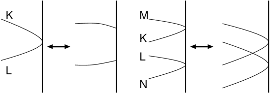
Figure 7: Open string interaction

The intereting problem for the future work is as follows. The description of the second-quantized superstring theory is discussed in a slightly different way.[36] The fermionic ${\bf Z}_{2}$-twisting is identified with the $H^{2}(S_{N},U(1))$, and the supersymmetry is described in more compact way. The consideration for the open string in this context will be interesting. The other direction is the non-trivial background. Recently the string theory in the non-commutative geometry has been developing.[37] The Matrix string theory in the B-field background is also discussed.[18] Whether the open string theory on the symmetric product of the non-commutative geomtry naturally describes the string field theory in the non-commutative geometry is very interesting issue. Furthermore, the matrix model is discussed in the Melvin background.[38] The extension of our model to this background will be also interesting. The string theory on the symmetric product of the curved background as Calabi-Yau manifold was partially discussed.[39] We expect that the construction of the boundary states which represent the D-branes wrapping around the supersymmetric cycle or holomorphic cycle may shed new light on the string field theory on the Calabi-Yau manifolds[40, 41] and the open string instanton calculations.[42]

Acknowledgement: The author is obliged to Y.Matsuo for his useful suggestions.

The author is supported by the JSPS fellowship for Young Scientist.

References

• [1] H.Fuji and Y.Matsuo, “Open String on Symmetric Product”,
Int.J.Mod.Phys.A16 (2001) 557-608, hep-th/0005111.
• [2] M.Kaku and K.Kikkawa, “Field Theory of Relativistic Strings. I. Trees”, Phys.Rev.D10 (1974) 1110-1133; “Field Theory of Relativistic Strings. II. Loops and Pomerons”, Phys.Rev.D10 (1974) 1823-1843.
• [3] E.Cremmer and J.L.Gervais, “Combining and Splitting Relativistic Strings”, Nucl.Phys.B76 (1974) 209-230; “Infinite Component Field Theory of Interacting Relativistic Strings and Dual Theory”, Nucl.Phys.B90 (1975) 410-460.
• [4] E.Witten, “Non-commutative Geometry and String Field Theory”, Nucl.Phys.B268 (1986) 79-324;
“Interacting Field Theory of Open Superstring Field Theory”,
Nucl.Phys.B276 (1986) 291-324.
• [5] H.Hata, K.Itoh, T.Kugo, H.Kunitomo and K.Ogawa, “Covariant String Field Theory”, Phys.Rev.D34 (1986) 2360-2429; “Covariant String Field Theory, II”, Phys.Rev.D35 (1987) 1318-1355.
• [6] S.Mandelstam, “Interacting-String Picture of the Neveu-Schwarz-Ramond Model”, Nucl.Phys.B69 (1974) 77-106; “Lorentz Properties of The Three-String Vertex”, Nucl.Phys.B83 (1974) 413-439.
• [7] M.B.Green and J.H.Schwarz, “Superstring Interactions”, Nucl.Phys.B218 (1983) 43-88; “Superstring Field Theory”, Nucl.Phys.B243 (1984) 475-536.
• [8] N.Berkovits, “Super-Poincare Invariant Superstring Field Theory”, Nucl.Phys.B450 (1995) 90-102, hep-th/9503099.
• [9] T.Banks, W.Fischler, S.H.Shenker and L.Susskind, “M Theory As A Matrix Model:A Conjecture”,Phys.Rev.D55 (1997) 5112-5128, hep-th/9610043.
• [10] R.Dijkgraaf, E.Verlinde and H.Verlinde, “Matrix String Theory”, Nucl.Phys.B500 (1997) 43-61, hep-th/9703030.
• [11] L.Motl, “Proposals on Nonperturbative Superstring Interactions”, hep-th/9701025.
• [12] T.Banks and N.Seiberg, “Strings from Matrices”, Nucl. Phys. B497 (1997) 44-55, hep-th/9702187.
• [13] R.Dijkgraaf, G.Moore, E.Verlinde and H.Verlinde, “Elliptic Genera of Symmetric Products and Second Quantized Strings”, Commun.Math.Phys. 185 (1997) 197-209, hep-th/9608096.
• [14] L.Susskind, “Another Conjecture about M(atrix) Theory”, hep-th/9704080,
• [15] P.Bantay, “Characters and modular properties of permutation orbifolds”, Phys.Lett.B419 (1998) 175-178, hep-th/9708120; “Permutation orbifolds”, hep-th/9910079; Z.Kadar, “The torus and the Klein Bottle amplitude of permutation orbifolds”, Phys.Lett.B484 (2000) 289-294, hep-th/0004122.
• [16] I.Kostov and P.Vanhove, “Matrix String Partition Functions”, Phys.Lett.B444 (1998) 196-203, hep-th/9809130; C.Bachas, C.Fabre, E.Kiritsis, N.A.Obers, and P.Vanhove, “Heterotic / type I duality and D-brane instantons”, Nucl.Phys.B509 (1998) 33-52, hep-th/9707126.
• [17] F.Sugino, “Cohomological Field Theory Approach to Matrix Strings” Int.J.Mod.Phys.A14 (1999) 3979-4002, hep-th/9904122.
• [18] G.Griani, M.Orsel and Semenoff, “Matrix strings in a B-field”,JHEP.0107 (2001) 004, hep-th/0104112.
• [19] L.Smolin, “M theory as a matrix extension of Chern-Simons theory”, Nucl.Phys.B591 (2000) 227-242; “The cubic matrix model and a duality between strings and loops”, hep-th/0006137; “The exceptional Jordan algebra and the matrix string”, hep-th/0104050.
• [20] F.Sugino and P.Vanhove, “ U-duality from Matrix Membrane Partition Function”, Phys.Lett.B522 (2001) 145-154, hep-th/0107145.
• [21] Y.Sekino and T.Yoneya, “From Supermembrane to Matrix String”, Nucl.Phys.B619 (2001)22-50, hep-th/108176.
• [22] Clifford V.Johnson, “On Second-Quantized Open Superstring Theory”,
Nucl.Phys.B537 (1999) 144-160, hep-th/9806115.
• [23] J.Polchinski, “String Theory I,II”, Cambridge University Press (1998).
• [24] S.Lang, “Introduction to Modular Forms ”, Graduate Texts in Mathematics 222, Springer-Verlarg (1976).
• [25] J.-P.Serre, “A Course in Arithmetics”, Graduate Texts in Mathematics 7, Springer-Verlag (1973).
• [26] T.M.Apostol, “Modular Functions and Dirichlet Series in Number Theory”, Graduate Texts in Mathematics 41, Springer-Verlarg (1976).
• [27] G.Pradisi and A.Sagnotti, “Open String Orbifolds”, Phys.Lett.B216 (1989) 59-67.
• [28] N.Ishibahi and T.Onogi, “Open String Model Building”, Nucl.Phys.B318 (1989) 239.
• [29] J.A.Harvey and J.A.Minahan, “Open Strings on Orbifolds”, Phys.Lett.B188 (1987) 44-50.
• [30] Y.Cai and J.Polchinski, “Consistency of the Open Super String”, Nucl.Phys.B296 (1988) 91-128.
• [31] G.E.Arutyunov and S.A.Frolov, “Virasoro amplitude from the $S^{N}{\bf R}^{24}$ orbifold sigma model”, Theor.Math.Phys.114 (1998) 43-66, hep-th/9708129.
• [32] G.E.Arutyunov and S.A.Frolov, “Four graviton scattering amplitude from $S^{N}{\bf R}^{8}$ supersymmetric orbifold sigma model”, Nucl.Phys.B524 (1998) 159-206, hep-th/9712061; G.Arutyunov, S.Frolov and A.Polishchuk “On Lorentz invariance and supersymmetry of four particle scattering amplitudes in $S^{N}{\bf R}^{8}$ orbifold sigma model”, Phys.Rev.D60 (1999) 066003, hep-th/9812119.
• [33] H.Fuji, Ph.D thesis in University of Tokyo, 2002.
• [34] A. Sen and B. Zwiebach, “Tachyon condensation in string field theory” JHEP0003 (2000) 002, hep-th/9912249.
• [35] N. Berkovits, A. Sen and B. Zwiebach, “Tachyon condensation in superstring field theory”, Nucl.Phys.B587 (2000) 147-178. hep-th/0002211.
• [36] R.Dijkgraaf, “Discrete Torsion and Symmetric Products”, hep-th/9912101.
• [37] N.Seiberg and E.Witten, “String Theory and Noncommutative Geometry”, JHEP 9909 (1999) 032, hep-th/9908142.
• [38] L.Motl, “Melvin Matrix Models”, hep-th/0107002.
• [39] A.Klemm and M.G.Schmid, “Orbifolds by Cyclic Permutations of Tensor Product Conformal Field Theories”, Phys.Lett.B245 (1990) 53-58; J.Fuch, A.Klemm and M.G.Schmid, “Orbifolds by Cyclic Permutations in Gepner Type Superstrings and in the Corresponding Calabi-Yau Manifolds”, Annals. Phys.214 (1992) 221-257.
• [40] E.Witten, “Chern-Simons Theory As A String Theory”, hep-th/9207094.
• [41] N.Berkovits, “Covariant Quantization of the Green-Schwarz Superstring in a Calabi-Yau Background”, Nucl.Phys.B431 (1994) 258-272, hep-th/9404162; “Review of Open Superstring Field Theory”, hep-th/0105230; “The Ramond Sector of Open Superstring Field Theory”, hep-th/0109100.
• [42] T.Kawai and K.Yoshioka, “String Partition Functions and Infinite Products”,
Adv.Theor.Math.Phys. 4 (2001) 397-485, hep-th/0002169.