Abstract

We provide examples of gravitational collapse and black hole formation in AdS, either from collapsing matter shells or in analogy to the Oppenheimer-Sneider solution. We then investigate boundary properties of the corresponding states. In particular, we describe the boundary two-point function corresponding to a shell outside its horizon; if the shell is quasistatically lowered into the horizon, the resulting state is the Boulware state. We also describe the more physical Hartle-Hawking state, and discuss its connection to the quasistatic shell states and to thermalization on the boundary.

1 Introduction

The problem of quantizing gravity is perhaps most sharply focussed in the question of what happens to quantum-mechanical information that falls into a black hole. Attempts to envision an answer have lead to the black hole information paradox. A proposed resolution to the paradox that saves unitary quantum evolution emerges from the ideas of holography[5, 6]: information escapes from the black hole by non-local mechanisms unique to gravity, and can be equivalently described as being stored on the surface of the hole. A concrete proposal for how holography works is found in the conjectured AdS/CFT correspondence[7], which states that string theory in the bulk of $AdS_{5}\times S^{5}$ is equivalent to an ${\cal N}=4$ supersymmetric gauge theory on the boundary.

If the conjecture of [7] is correct, then the gauge theory should be capable of describing the formation and subsequent evaporation of a black hole, and should in particular furnish a unitary description of that process. Understanding how this happens would conclusively solve the black hole information paradox.

So far, however, it has been difficult to find such a concrete resolution. The translation between bulk and boundary physics is only partially understood; for example, it is known that correlators in the boundary theory can be obtained from a bulk generating functional[8, 9], and conversely, that a bulk analog of the S-matrix (called the “boundary S-matrix” in [10]) can be readily obtained from the boundary correlators[11, 10]. However, a difficult unresolved problem has been to extract physics on scales less than the AdS radius $R$ (or, equivalently to find the flat space S-matrix) from this boundary S-matrix; attempts have been made in [12, 13], but difficulties in obtaining flat-space physics have been pointed out in [14].

An alternate approach to trying to reconstruct directly the flat-space dynamics is to attempt to diagnose properties of non-trivial bulk states using correlators on the boundary. One might for example consider a configuration undergoing gravitational collapse to form a black hole that subsequently evaporates, and ask what correlation functions of boundary operators tell us about the corresponding evolution of the gauge-theory state on the boundary. Better understanding of this state is particularly relevant in confronting the information problem. The boundary description of a black hole formed from a pure state is an apparently thermal state[9, 15], but in the present thinking is expected to be a fundamentally pure state. The information hidden in this apparently thermal boundary state is the same as the information hidden in the black hole in the bulk description. Therefore understanding how the state approaches the apparently thermal state and how this information is encoded – and whether it might be accessed – should be equivalent to understanding how information is hidden inside a black hole, and how it might be accessed, or radiated in the Hawking radiation. Other discussions of the correspondence between falling into a black hole and thermalization on the boundary have previously been given in [16, 17].

Some preliminary aspects of the boundary description of gravitational collapse have been investigated in [18, 19] in the case of collapse of a shell of D3 branes (corresponding to a configuration on the Coulomb branch) to a black brane. However, the surface of this problem has just been scratched. In particular, consider a family of solutions consisting of shells of three branes with progressively smaller radii. In the limit when the three branes coincide, we have a macroscopic extremal black three brane. This limit was examined by Ross and one of the present authors in [19], which in particular investigated properties of two point functions and Wilson loops in the boundary description of the configuration. For any finite shell radius a discrete spectrum of boundary states was found, although it was argued that absorption effects on the shell would broaden these states. In the limit when the shell reaches the horizon, these states merge into the continuum appropriate for describing AdS in Poincaré coordinates.

We’d like to understand this transition better. It particularly becomes puzzling when we discuss infalling observers. For any finite radius shell, the interior of the shell is flat space, and an infalling observer will have to penetrate the shell in order to travel beyond. However, the exterior of the zero-radius shell is the Poincaré patch of AdS space, and we believe an infalling observer can sail through the horizon and explore points beyond. An important goal is to understand the relationship between these two pictures.

Of course physically speaking this story is not quite complete. In order to bring the individual D3 branes together we must give them a slight velocity. This raises the system above extremality, and a horizon will form somewhat outside the extremal horizon; the presumed Penrose diagram for this process was sketched in [19]. However, this does not lessen the puzzle. From the point of view of the gauge theory, the coalescing D3 branes corresponds to time dependent vevs on the Coulomb branch. Presumably horizon formation corresponds to thermalization of this time dependent state. However, we should also be able to describe the observations of an infalling observer, and after the horizon has formed this observer will see another region of space – behind the horizon – open up for exploration. The “dual” description of this physics in the gauge theory is far from apparent. In order to better understand the black hole information paradox, we want to get at the root of black hole complementarity and learn more about the map between internal degrees of freedom of the black hole and their boundary description.

We do not yet even have the starting point of classical solutions for collapsing D3 branes, but related problems exist if we return to the context of a collapsing black hole. For example, one can consider, in an asymptotically AdS space, a configuration of particles that undergoing gravitational collapse. A first set of questions is how to use boundary correlators to diagnose properties of the corresponding boundary state. An obvious quantity to consider is the boundary stress tensor, but in spherically symmetric collapse its expectation value is constant by Birkhoff’s theorem. One must use finer diagnostics – for example two- and higher-point functions.

This paper will make some modest progress towards addressing the question of black hole formation and the corresponding boundary thermalization. In particular, we will consider idealized configurations of matter – collapsing shells – and discuss aspects of their boundary description and the question of thermalization.

In outline, the next section will discuss the classical collapse, in AdS, of a shell of dust. (The similar problem of Oppenheimer-Snyder collapse of a ball of dust is discussed in the appendix.) We then turn towards finding the boundary description of this configuration. We wish to probe some of its properties via the bulk-boundary correspondence for a minimally coupled scalar field moving in such a background. Even this problem is somewhat complicated, so we warm up with the simpler problem of computing the boundary two-point function for a shell that we quasistatically lower to the horizon. Specifically, in section three we quantize the scalar in this background, and see that this has similar features to the D3 brane shells, in particular a discrete spectrum of states. In the limit as the shell approaches the horizon, we show that these merge into a continuum and we recover the Boulware state. In contrast to this, the correct vacuum to describe a black hole is the Hartle-Hawking state, which we describe in section four. The transition between the state with a shell just outside the horizon and the Hartle-Hawking state appears to be a difficult dynamical problem which we still lack the tools to address. We close with discussion of this problem and the corresponding problem for D3 branes. For related comments on eternal black holes in AdS see [20].

2 A collapsing shell in AdS

We will be working in the $d+1$ dimensional spacetime of signature $(-,+,...+)$, with action

$$S=\frac{1}{16\pi G}\int d^{d+1}x\sqrt{-g}(R-\Lambda)+\int d^{d+1}x\sqrt{-g}{\cal L}_{m}$$ (2.1)

where ${\cal L}_{m}$ is the matter lagrangian. Einstein’s equation are

$$R_{\mu\nu}-{1\over 2}g_{\mu\nu}R=\kappa T_{\mu\nu}-{\Lambda\over 2}g_{\mu\nu}\$$ (2.2)

with $\kappa=8\pi G$. The vacuum solution is anti-de Sitter space, which in global coordinates has metric

$$ds^{2}=-(1+r^{2}/b^{2})dt^{2}+dr^{2}/(1+r^{2}/b^{2})+r^{2}d\Omega_{d-1}^{2}$$ (2.3)

with

$$b^{2}=-\frac{d(d-1)}{\Lambda}\ .$$ (2.4)

In order to study gravitational collapse in AdS, we consider a particularly simple configuration: a shell of dust, which collapses to form a black hole. We can think of this as an idealization of a collection of particles (e.g. dilatons or massive particles) distributed over a thin inward-moving shell. Such shells have been previously considered in this context in [22, 23].

The energy momentum tensor for a spherically-symmetric shell of pressureless dust following a radial trajectory $R(\tau)$ and with density $\sigma$ is given by

$$T_{\mu\nu}=\sigma U_{\mu}U_{\nu}\delta(r-R(\tau))\ ,$$ (2.5)

where $U^{\mu}$ is the velocity of the shell, which satisfies $U^{\mu}U_{\mu}=-1$. Inside the shell the metric is that of global AdS,

$$ds^{2}=-{f_{-}}(r)dt_{-}^{2}+dr^{2}/{f_{-}}(r)+r^{2}d\Omega_{d-1}^{2}\ ,$$ (2.6)

where

$${f_{-}}(r)=1+{r^{2}\over b^{2}}\ .$$ (2.7)

The external metric is Schwarzschild-AdS:

$$ds^{2}=-{f_{+}}(r)d{t_{+}}^{2}+dr^{2}/{f_{+}}(r)+r^{2}d\Omega_{d-1}^{2}\$$ (2.8)

with

$${f_{+}}(r)=1+{r^{2}\over b^{2}}-{m\over r^{d-2}}\ .$$ (2.9)

Here the mass parameter $m$ is related to the mass by

$$M_{ADM}={(d-1)\Omega_{d-1}\over 16\pi G}m\ ,$$ (2.10)

with $\Omega_{d-1}$ the area of the unit $d-1$ sphere, and the Schwarzschild radius is given by

$$m=r_{H}^{d-2}(1+\frac{r_{H}^{2}}{b^{2}})\ .$$ (2.11)

The Penrose diagram for Schwarzschild-AdS is shown in fig. 1.

Figure 1: The Penrose diagram for Schwarzschild-AdS.

The induced metric on the surface of the shell should be the same computed from the inside or outside metric. In addition, if the shell is freely falling, its motion is determined by matching the extrinsic curvature of the geometry across the shell. The first condition relates time inside and outside the shell:

$${d{{t_{-}}}\over d{t_{+}}}=\sqrt{{f_{+}}\over{f_{-}}}\ .$$ (2.12)

The matching conditions for the extrinsic curvature are the Israel matching conditions[24]. These take the form

$$K^{+}_{ab}-K^{-}_{ab}=-\kappa\sigma\left(U_{a}U_{b}+{g_{ab}\over 2}\right)$$ (2.13)

$$(K^{+}_{ab}+K^{-}_{ab})U^{a}U^{b}=0\$$ (2.14)

where latin indices denote indices tangent to the shell’s world-volume, and $K_{ab}$ is the extrinsic curvature of the shell’s world-volume. These equations can be thought of as summarizing the balance of normal forces on the shell’s surface layer. Let $n^{\mu}$ denote the normal vector to an infinitesimal element of the shell. One can readily show that the geodesic equation of this element implies[24, 25]

$$n_{\mu}{DU^{\mu}\over d\tau}|_{\pm}=-K_{ab}^{\pm}U^{a}U^{b}\ .$$ (2.15)

Combining this equation with (2.13), (2.14) then gives the equations

$$n_{\mu}\frac{DU^{\mu}}{d\tau}|_{+}+n_{\mu}\frac{DU^{\mu}}{d\tau}|_{-}=0\ ,$$ (2.16)

$$n_{\mu}\frac{DU^{\mu}}{d\tau}|_{+}-n_{\mu}\frac{DU^{\mu}}{d\tau}|_{-}={\kappa\sigma\over 2}\ .$$ (2.17)

In terms of the trajectory $R(\tau)$, the velocity and normal are easily seen to take the form

$$U^{\mu}_{\pm}=(\dot{t}_{\pm},\dot{R},0,\ldots,0)\ ,\ n^{\pm}_{\mu}=(-\dot{R},\dot{t}_{\pm},\ldots,0)$$ (2.18)

where

$$\dot{t}_{\pm}=\sqrt{f_{\pm}(r)+\dot{R}^{2}}/f_{\pm}(R)\ .$$ (2.19)

Given these expressions and the metric (2.6), (2.8), we may evaluate the left hand sides of (2.16), (2.17), and derive a differential equation whose first integral of the motion is

$$1+\left(\frac{dR}{d\tau}\right)^{2}+\left(\frac{R}{b}\right)^{2}=\left(a+\frac{m}{4aR^{d-2}}\right)^{2}\\$$ (2.20)

where $a$ is an integration constant. The rest mass of the shell, if infinitely dispersed, is

$$M={m\Omega_{d-1}(d-2)\over\kappa a}\ .$$ (2.21)

In Minkowski space ($b\rightarrow\infty$) an expanding shell escapes to infinity if $a>1$ and rebounds at finite radius if $a<1$. In AdS, all expanding shells clearly rebound at some finite radius.

The collapsing shell crosses the horizon when $f_{+}(R)=0$, and thus forms a black hole, as shown in fig. 2.

Figure 2: The Penrose diagram for collapsing shell in anti de-Sitter space.

We would like to better understand the boundary CFT representation of this process.

The coarsest diagnostic of a configuration in AdS is its boundary stress tensor. While many configurations in AdS have a non-trivial boundary stress tensor which encodes important data about the bulk state, by Birkhoff’s theorem all spherically symmetric solutions in AdS are asymptotically of the form (2.8) and thus have the same stress tensor [26],

$$T_{\mu\nu}=\rho\left(t_{\mu}t_{\nu}\ +{1\over{d-1}}h_{\mu\nu}\right),$$ (2.22)

where $t^{\mu}$ is the unit timelike Killing vector on the boundary of Schwarzschild-AdS, $h_{\mu\nu}$ is the metric on $S^{d-1}$, and $\rho$ is the mass density on the boundary. The latter is related to bulk quantities by

$$\rho=\frac{r_{H}}{\kappa b^{2}}$$ (2.23)

for $d=3$, and

$$\rho=\frac{3}{8\kappa b^{3}}(b^{2}+4r_{H}^{2})$$ (2.24)

for $d=4$. Thus in particular, the boundary stress tensor does not distinguish between a black hole and a collapsing shell. For this reason we must seek refined diagnostics to distinguish these configurations. Perhaps the simplest such example is the two-point function of fields propagating in the bulk background, and the corresponding boundary correlator.

3 Quantization in the shell background

3.1 Classical solutions

We next turn to the quantization of fields moving in the background of a shell; for simplicity we consider a minimally coupled scalar field,

$$\Box\phi=0.$$ (3.1)

Also for simplicity, we consider solutions to this equation in the background of a static shell fixed at constant $R$; this is of course a good approximation for the slowly-moving shell, but not for example for a shell crossing a horizon. We can alternately consider a quasistatic (non-geodesic) family of shells that gradually approaches the horizon; although such a family would have to be accelerated by an external agent, study of the corresponding bulk and boundary states is hoped to yield further insight into gravitational collapse.

The solutions to (3.1) in the shell background are not known, but we will infer some of their properties. We are particularly interested in the spectrum, and other properties of the state as the horizon forms.

In order to study eq. (3.1), we will write the metric (2.6), (2.8) both inside and outside the shell in the uniform form

$$ds^{2}=-\tilde{f}(r)dt^{2}+\frac{dr^{2}}{f(r)}+r^{2}d\Omega^{2}$$ (3.2)

where

$$f = 1+r^{2}$$ (3.3)

$$\tilde{f} = (1+r^{2})\frac{(1-m/R^{d-2}+R^{2})}{1+R^{2}}$$ (3.4)

for $r<R$ and

$$\tilde{f}=f=1-m/r^{d-2}+r^{2}$$ (3.5)

for $r>R$. Here and for the rest of the section we work in units in which the AdS radius $b=1$. Notice in particular that while (3.4) corresponds to unperturbed AdS, the extra factor accounts for a relative redshift: a given proper frequency measured by an observer in the center of the AdS portion corresponds to a redshifted frequency as seen by an asymptotic observer.

We consider a solution of (3.1) of definite frequency and angular momentum,

$$\phi=\varphi_{\omega l{\vec{m}}}(r)e^{-i\omega t}Y_{l{\vec{m}}}\ .$$ (3.6)

Properties of such solutions are most easily understood by introducing the tortoise coordinate $r_{*}$,

$$dr_{*}=\frac{dr}{\sqrt{f\tilde{f}}}\ ,$$ (3.7)

in terms of which the $t$, $r$ part of the metric takes conformally flat form. We also rescale the wavefunction,

$$\varphi_{\omega l{\vec{m}}}(r)={u_{\omega l{\vec{m}}}\over r^{(d-1)/2}}\ .$$ (3.8)

In these variables the radial solution to the wave equation is found by solving a one-dimensional potential problem,

$$\frac{d^{2}u_{\omega l{\vec{m}}}}{dr_{*}^{2}}+(\omega^{2}-V_{eff})u_{\omega l{\vec{m}}}=0$$ (3.9)

with effective potential given by

$$V_{eff}=\frac{\tilde{f}l(l+d-2)}{r^{2}}+\left(\frac{d-1}{2}\right){1\over 2r}\frac{d(f\tilde{f})}{dr}+\left(\frac{d-1}{2}\right)\left(\frac{d-3}{2}\right)\frac{f\tilde{f}}{r^{2}}\ .$$ (3.10)

The solutions should of course be continuous at the shell; integrating (3.9) then yields the matching condition

$$\frac{du_{\omega l{\vec{m}}}}{dr_{*}}|_{+}-\frac{du_{\omega l{\vec{m}}}}{dr_{*}}|_{-}$$ (3.11)

$$=u_{\omega l{\vec{m}}}(R){d-1\over 2R}\sqrt{1-\frac{m}{R^{d-2}}+R^{2}}\left(\sqrt{1-\frac{m}{R^{d-2}}+R^{2}}-\sqrt{1+R^{2}}\right).$$

This equation is easily seen to correspond to the condition that the normal derivatives match across the shell,

$$n^{\mu}\nabla_{\mu}\phi|^{+}-n^{\mu}\nabla_{\mu}\phi|^{-}=0\ .$$ (3.12)

Note that both our effective potential (3.10) and boundary conditions (3.11), (3.12) differ from those in [23]. For example, [23] replaces the interior of the shell by the Poincaré patch of AdS.

The potential (3.10) takes the form shown in fig. 3; inside the shell it is the potential of unperturbed AdS – with additional redshift – and outside it is that of Schwarzschild-AdS. The solutions will have quantized frequencies $\omega_{n}$.

Figure 3: The effective potential for $d=4$, $l=0$, $r_{H}=2$ and $R=5$. The shell lies at $r_{*}\approx 1.37$ and produces a delta function in the potential, as shown.

To see the effects of the shell on the spectrum, first consider the situation where the shell is far from the horizon. This case is most easily analyzed by working in the proper time coordinate of the central observer, which is

$${\hat{t}}=\sqrt{\frac{(1-m/R^{d-2}+R^{2})}{1+R^{2}}}t\ .$$ (3.13)

In this coordinate the metric takes the form

$$ds^{2}=-\tilde{f}(r)d{\hat{t}}^{2}+\frac{dr^{2}}{f(r)}+r^{2}d\Omega^{2}\ ,$$ (3.14)

where for $r<R$

$$f=\tilde{f}=1+r^{2}$$ (3.15)

and for $r>R$

$$f=1-{m\over r^{d-2}}+r^{2}\ ,\ \tilde{f}=(1-\frac{m}{r^{d-2}}+r^{2})\frac{1+R^{2}}{1-\frac{m}{R^{d-2}}+R^{2}}\ .$$ (3.16)

The wave equation then becomes

$$\frac{d^{2}u_{nl{\vec{m}}}}{dr_{*}^{2}}+(\hat{\omega}^{2}-V_{eff})u_{nl{\vec{m}}}=0\$$ (3.17)

where $V_{eff}$ is found as in (3.10). This can be solved for the characteristic frequencies $\hat{\omega}_{n}$; the frequencies seen by the asymptotic observer are then given by

$$\omega_{n}=\sqrt{\frac{(1-m/R^{d-2}+R^{2})}{1+R^{2}}}\hat{\omega}_{n}\ .$$ (3.18)

The resulting effective potential can be written as that of AdS, plus a perturbation,

$$V_{eff}=V_{AdS}+V_{m}\ .$$ (3.19)

The unperturbed eigenfunctions of the AdS wave operator take the form

$$u_{nl}(r_{*})=c_{nl}\cos^{\frac{1+d}{2}}(r_{*})\sin^{\frac{d-1+2l}{2}}(r_{*})P_{n}^{l-1+\frac{d}{2},{d\over 2}}(\cos 2r_{*})\ ,$$ (3.20)

where $c_{nl}$ are normalization constants, and have quantized frequencies

$${\hat{\omega}}_{nl}=d+l+2n\ .$$ (3.21)

For $r<R$, the metric is precisely of AdS form, so $V_{m}$=0 for $r<R$. The perturbation for $r>R$ is bounded as

$$|V_{m}|\raise 1.29167pt\hbox{$<$\kern-7.5pt\lower 4.30554pt\hbox{$\sim$}}\frac{m}{R^{d-2}}\ .$$ (3.22)

Using $dr_{*}\sim dr/r^{2}$, $u\sim\frac{1}{r^{(d+1)/2}}$ and (3.22), we obtain the shift in frequency as seen by an AdS observer:

$$|\Delta\hat{\omega}|\raise 1.29167pt\hbox{$<$\kern-7.5pt\lower 4.30554pt\hbox{$\sim$}}\frac{m}{R^{2d}}\ .$$ (3.23)

This shows that the contribution of the $r>R$ perturbation to the effective potential is subleading to the redshift contribution (3.18). An additional contribution to the effective potential comes from the delta function at $r=R$:

$$V_{m}=-\frac{(d-1)m}{4R^{d-1}}(1+R^{2})\delta(r-R)\ .$$ (3.24)

This gives a contribution ${\cal O}\left(\frac{m}{R^{2d}}\right)$ to $\Delta\hat{\omega}$ which is again subleading. Thus to leading order in $\frac{1}{R}$, we find that the frequencies seen by the outside observer are shifted homogeneously as

$$\Delta\omega_{nl{\vec{m}}}=-\frac{m}{2R^{d}}\omega_{nl{\vec{m}}}\ .$$ (3.25)

The net effect is a redshift of the eigenfrequencies of the modes. While this perturbative analysis will fail as the shell approaches the horizon, the qualitative effect remains the same, namely increasing redshift for decreasing radius. When the shell reaches the horizon, the modes of the internal AdS region are infinitely redshifted, and the outside observer sees the emergence of a continuum. This is clear from the form of the effective potential; as $R$ approaches the horizon, the shell moves to $r_{*}=-\infty$, and the potential takes the form shown in fig. 4.

Figure 4: The effective potential for $d=4$, $l=0$,$r_{h}=2$ and $R=2.01$. The shell is close to its gravitational radius. Note that the potential in the vicinity of the shell is very small as compared to the case of a large-radius shell, fig. 3. It has also been shifted leftwards; now the shell lies at $r_{*}\approx 0.7$.

Figure 5: Tortoise coordinate $r_{*}$ position of the shell as a function of $R$. Note that the shell moves to $r_{*}=-\infty$ as $R\rightarrow r_{H}=2$.

3.2 Quantization

Given the limitations of the stress tensor as a diagnostic of properties of a collapsing configuration, we next turn to the calculation of the two-point function. This proceeds via canonical quantization of the field $\phi$. In particular, $\phi$ can in general be expanded in a general orthonormal basis of modes $\left\{\phi_{\alpha}\right\}$ as

$$\phi=\sum_{\alpha}\left(\phi_{\alpha}a_{\alpha}+\phi_{\alpha}^{*}a_{\alpha}^{\dagger}\right)$$ (3.26)

where $a_{\alpha}$, $a_{\alpha}^{\dagger}$ are the corresponding annihilation and creation operators. Definition of such a basis and corresponding ladder operators also serves to define a vacuum,

$$a_{\alpha}|0\rangle=0\ .$$ (3.27)

The two-point function is then given by

$$\langle\phi(x)\phi(y)\rangle=\langle 0|T\left[\phi(x)\phi(y)\right]|0\rangle\ .$$ (3.28)

Choosing the basis $\left\{\phi_{\alpha}\right\}=\left\{\varphi_{nl{\vec{m}}}e^{-i\omega t}Y_{l{\vec{m}}}/\sqrt{2\omega_{nl}}\right\}$ given in the last subsection therefore defines a vacuum $|0\rangle_{\rm shell}$ and two-point function for the shell configuration. The latter takes the form

$$\langle\phi(x)\phi(x^{\prime})\rangle_{\rm shell} = {1\over i}\sum_{nl\vec{m}}Y_{l{\vec{m}}}({\hat{e}})Y^{*}_{l{\vec{m}}}({\hat{e}}^{\prime})\int\frac{d\omega}{2\pi}e^{-i\omega(t-t^{\prime})}\frac{\varphi_{nl\vec{m}}(r)\varphi^{*}_{nl\vec{m}}(r^{\prime})}{\omega_{nl}^{2}-\omega^{2}-i\epsilon}$$ (3.29)

$$= \theta(t-t^{\prime})s(x,x^{\prime})+\theta(t^{\prime}-t)s^{*}(x,x^{\prime})$$

where ${\hat{e}}$ and ${\hat{e}}^{\prime}$ are unit vectors giving the directions of $\vec{x}$ and ${\vec{x}}^{\prime}$, and

$$s(x,x^{\prime})=\sum_{nl\vec{m}}Y_{l{\vec{m}}}({\hat{e}})Y^{*}_{l{\vec{m}}}({\hat{e}}^{\prime}){e^{-i\omega_{nl}(t-t^{\prime})}\over 2\omega_{nl}}\varphi_{nl{\vec{m}}}(r)\varphi_{nl{\vec{m}}}^{*}(r^{\prime})\ .$$ (3.30)

One way of characterizing a vacuum is in terms of local observations performed, for example, by an observer carrying an Unruh detector [27]. Recall that an Unruh detector can be thought of as a simple quantum-mechanical system, e.g. a harmonic oscillator carried by a local observer. The harmonic oscillator lagrangian contains a coupling to the field of the form

$$S_{I}=\int d\tau Z(\tau)\phi(x(\tau))\ ,$$ (3.31)

where $Z$ is the oscillator position variable, and $\tau$ is the proper time along the observer’s worldline $x(\tau)$. In the vacuum $|0\rangle_{shell}$ defined by the shell modes, an Unruh detector carried by an observer following a trajectory of constant $r$ stays unexcited.

Indeed, in the limit as the shell approaches the horizon, the state $|0\rangle_{shell}$ approaches another well known state, the Boulware vacuum. With the shell at the horizon, the wave equation (3.1) is simply the wave equation in the Schwarzschild-AdS background. Working in the coordinates $t,r_{*}$, we derive the effective potential for Schwarzschild-AdS; in particular, Schwarzschild time $t$ defines a notion of positive frequency, and the resulting Boulware modes $\varphi_{\omega l{\vec{m}}}^{B}e^{-i\omega t}Y_{l{\vec{m}}}$ define the Boulware vacuum,

$$a_{\omega l{\vec{m}}}^{B}|0\rangle_{B}=0\ .$$ (3.32)

As in the shell case, observers at constant $r$ do not see particles in this state.

3.3 Boundary description

According to the prescription of [8, 9], the two-point function of the boundary operator $\cal O$ corresponding to the field $\phi$ is obtained as a rescaling of the limit of the two-point function (3.28) as its arguments go to the boundary. The rescaling needed follows from the asymptotic form of the normal modes $\phi_{nl{\vec{m}}}$. In particular, this asymptotic form depends on the AdS radius but not the black hole mass, and we find

$$\phi_{nl{\vec{m}}}\rightarrow{{k}_{nl}\over\sqrt{2\omega_{nl}}}\frac{1}{r^{d}}Y_{l{\vec{m}}}e^{-i\omega_{nl}t}$$ (3.33)

with ${k}_{nl}$ constants given in [14]. Thus the boundary two-point function takes the form

$$\langle{\cal O}(b){\cal O}(b^{\prime})\rangle\propto \lim_{r,r^{\prime}\rightarrow\infty}(rr^{\prime})^{d}\langle\phi(x)\phi(x^{\prime})\rangle$$ (3.34)

$$={1\over i}\int{d\omega\over 2\pi}\sum_{nl{\vec{m}}}e^{-i\omega(t-t^{\prime})}k_{nl}^{2}{Y^{*}_{l{\vec{m}}}({\hat{e}})Y_{l{\vec{m}}}({\hat{e}}^{\prime})\over\omega_{nl}^{2}-\omega^{2}-i\epsilon}\ .$$

The spectrum of excitations on the boundary can of course be read off from the frequencies $\omega_{nl}$. As the shell reaches the horizon, these become continuous, corresponding to a continuum in the boundary theory. Similar behavior was found in [19] in the case of a shell of D3 branes collapsing into a black brane.

However, note that this shell vacuum is very different from the physical state we expect to form outside a black hole, which is described by the Hartle-Hawking state. In the case of extremal configuration of D3 branes, there is no corresponding issue – the Hawking temperature is zero, and the Boulware and HH states correspond. However, in the more physical non-extremal case of D3 branes with some initial velocity, as well as in the present case, the states are different. We would like to better understand the transition from one to another, and the corresponding boundary physics of thermalization. We begin by describing the HH state in more detail.

4 The Hartle-Hawking Green function and thermalization of the shell state

4.1 The Hartle-Hawking state and Green function for Schwarzschild-AdS

We begin by describing properties of the Hartle-Hawking (HH) state and Green function for Schwarzschild-AdS. Recall that there are several equivalent perspectives on the HH state and Green function.

In the first perspective, we chose a specific set of modes in the expansion of the field, (3.26), and define the vacuum to be annihilated by the corresponding annihilation operators. These modes are taken to have positive frequency with respect to an affine parameter along the horizon, or equivalently in the time defined in terms of Kruskal coordinates, that is, they are positive frequency as seen by a freely falling observer crossing the horizon.

In the case of Schwarzschild in a Minkowski background, one must in fact choose two sets of modes to form a basis. The first set can be defined to form a basis for solutions to the wave equation that vanish at past null infinity ${\cal I}_{-}$ and are purely positive frequency with respect to Kruskal time on the past horizon ${\cal H}_{-}$. The second set is a basis for solutions that vanish on ${\cal H}_{-}$ and are positive frequency with respect to Schwarzschild time at ${\cal I}_{-}$. Together these two sets of incoming modes form a basis for all solutions and define a vacuum. One may alternately define a basis of outgoing modes that is positive frequency at the future horizon ${\cal H}_{+}$ and future null infinity ${\cal I}_{+}$, and a corresponding vacuum.

In Schwarzschild-AdS, if we restrict to normalizable solutions, the boundary conditions mean that in the far past complete Cauchy data is specified on ${\cal H}_{-}$, or alternately in the far future it is specified on ${\cal H}_{+}$. In this case, we can choose a complete set of positive frequency modes on the past horizon, and define a corresponding vacuum $|0\rangle_{-}$. Alternately we may choose a basis that is positive frequency on the future horizon, and define a corresponding vacuum $|0\rangle_{+}$. The different definitions of the vacuum suggest an ambiguity in specifying the vacuum, and in defining the HH Green function. However, in [28] Gibbons and Perry use an analyticity argument to show that these are in fact the same vacuum for the Schwarzschild solution in a box; in the present case, AdS supplies a gravitational definition of a box. Thus $|0\rangle_{+}=|0\rangle_{-}\equiv|0\rangle_{HH}$, and the HH Green function is

$$G_{\rm HH}(x,x^{\prime})={}_{\rm HH}\langle 0|T\left[\phi(x)\phi(x^{\prime})\right]|0\rangle_{\rm HH}\ .$$ (4.35)

A second definition of the HH state and Green function follows the original paper [29] more directly. Continuing the complete Schwarzschild-AdS metric (2.8) to euclidean signature gives the metric

$$ds^{2}=f_{+}d\tau^{2}+dr^{2}/f_{+}+r^{2}d\Omega^{2}_{d-1}$$ (4.36)

with topology $R^{2}\times S^{d-1}$. Slicing this metric along the slice ${\cal S}$ of $\tau=0$, $\tau=\pi$ (see fig. 6) gives a spatial metric that agrees with spatial slices of constant Schwarzschild time in the full Kruskal extension of lorentzian Schwarzschild-AdS. A Green function may be defined directly on the euclidean manifold (4.36) and then its arguments may be analytically continued to points in lorentzian Schwarzschild-AdS. The result is again the HH Green function; equivalence follows from the analyticity properties of the continued lorentzian HH Green function, as discussed in [28].

Figure 6: Matching of Euclidean and lorentzian Schwarzschild-AdS. The corresponding spaces are identified along the surface ${\cal S}$.

A third, related, perspective sees the HH state and Green function as thermal with respect to observers traveling along trajectories of constant Schwarzschild radius $r$, whose proper time is $\propto t$. This thermal character is particularly simply elucidated in [30, 31], following earlier work of Israel[32] and Unruh[27]. In particular, the euclidean functional integral defines the HH state on the slice ${\cal S}$. A Schwarzschild observer sees only half of this slice; label the states seen by this observer as $|\phi_{R}\rangle$. To specify a state on the full slice ${\cal S}$, one must also specify the state $|\phi_{L}\rangle$ as seen by a Schwarzschild observer in the left quadrant, and so one can think of states on ${\cal S}$ as superpositions of states of the form $|\phi_{L}\phi_{R}\rangle$ in the tensor product Hilbert space. The euclidean functional integral defining the HH state can be written in terms of the Schwarzschild hamiltonian $H_{S}$ which generates evolution in the angular direction in the euclidean geometry, and so in the $L\times R$ basis the HH state takes the form

$$\langle\phi_{L}\phi_{R}|0\rangle_{\rm HH}\propto\langle\phi_{L}|e^{-\pi H_{S}}|\phi_{R}\rangle\ .$$ (4.37)

Since the HH Green function is the expectation value of operators defined in the right quadrant, this expectation value reduces to a trace over the left modes. This yields the thermal form for the Green function,

$${}_{\rm HH}\langle 0|T\left[\phi(x)\phi(x^{\prime})\right]|0\rangle_{\rm HH}\propto Tr\left(e^{-2\pi H_{S}}T\left[\phi(x)\phi(x^{\prime})\right]\right)\ .$$ (4.38)

Specifically, work in a basis for Schwarzschild modes of the form given in eq. (3.6). In this basis the HH Green function then takes a form originally given in [33]

$$G_{\rm HH}(x,x^{\prime})=\theta(t-t^{\prime})s_{\rm HH}(x,y)+\theta(t^{\prime}-t)s_{\rm HH}^{*}(x,y)$$ (4.39)

with

$$s_{\rm HH}(x,y) = \sum_{l\vec{m}}\int_{0}^{\infty}{d\omega\over 2\omega}\Biggl{[}\frac{e^{-i\omega(t-t^{\prime})}\varphi_{\omega l{\vec{m}}}(r)Y_{l{\vec{m}}}({\hat{e}})\varphi_{\omega l{\vec{m}}}^{*}(r^{\prime})Y_{l{\vec{m}}}^{*}({\hat{e}}^{\prime})}{1-e^{-\beta\omega}}$$ (4.40)

$$+ \frac{e^{i\omega(t-t^{\prime})}\varphi_{\omega l{\vec{m}}}^{*}(r)Y_{l{\vec{m}}}^{*}({\hat{e}})\varphi_{\omega l{\vec{m}}}(r^{\prime})Y_{l{\vec{m}}}({\hat{e}}^{\prime})}{e^{\beta\omega}-1}\Biggr{]}$$

and

$$\beta=\frac{4\pi r_{H}b^{2}}{dr_{H}^{2}+(d-2)b^{2}}\ .$$ (4.41)

The corresponding boundary Green function is derived as in (3.34) and takes the analogous form

$$\langle{\cal O}(b){\cal O}(b^{\prime})\rangle_{\rm HH}\propto\theta(t-t^{\prime})s_{\rm HH}(b,b^{\prime})+\theta(t^{\prime}-t)s_{\rm HH}^{*}(b,b^{\prime})$$ (4.42)

with

$$s_{\rm HH}(b,b^{\prime})=\sum_{l{\vec{m}}}\int{d\omega\over 2\omega}k_{\omega l}^{2}\left[{Y_{l{\vec{m}}}({\hat{e}})Y_{l{\vec{m}}}^{*}({\hat{e}}^{\prime})e^{-i\omega(t-t^{\prime})}\over 1-e^{-\beta\omega}}+{Y_{l{\vec{m}}}^{*}({\hat{e}})Y_{l{\vec{m}}}({\hat{e}}^{\prime})e^{i\omega(t-t^{\prime})}\over e^{\beta\omega}-1}\right]$$ (4.43)

where $k_{\omega l}$ are the continuum analogs of the constants defined in (3.33).

These Green functions clearly differ, by virtue of being thermal, from (3.29), (3.34) in the limit where the shell approaches the horizon.

4.2 Thermalization and approach to the Hartle Hawking state

The relationship between the shell/Boulware states that we have previously described and the Hartle-Hawking state that one expects to observe once a black hole has formed appear to be close to the heart of the black hole information paradox. In particular, the shell/Boulware state can be thought of as a pure state. We can imagine physically constructing it by quasistatically lowering steel plates close to the black hole horizon and bolting them together. However, if we sever the bolts, the shell collapses to a black hole which has as its external description the Hartle-Hawking state. This transition from an obviously pure state to an apparently thermal (but still presumably pure) state is expected to have a boundary description as a transition between a dynamical pure state and an apparent thermal state in the gauge theory. If we could explicitly describe this transition we would know where the information of the black hole is hidden, and may be able to better understand how it is revealed when the black hole evaporates.

It should also be noted that there is a direct relationship between the shell/Boulware state and the Hartle-Hawking state. In particular, Mukohyama and Israel[34] have argued that if one starts with a state of the shell/Boulware form and then adds on top of it thermal radiation to give what they call a “topped-up Boulware” state, this has the same properties (e.g. stress tensor, correlators) as the Hartle-Hawking state. In fact, this relationship is evident from (4.39) which exhibits the HH Green function as a thermal Green function in the basis appropriate to the Schwarzschild observer. The important question is how the state makes the transition from the shell/Boulware state to the Hartle-Hawking state. It is tempting to conjecture that this is by radiation from a collapsing shell, but we have not yet found a direct description of this process.

5 Discussion

The dynamical shell problem remains difficult. The shell/Boulware state and HH state are very different, and it is not obvious how to physically connect them. The problem of studying the dynamical shell is akin to a moving mirror problem [35], and perhaps further insight can be gained from studies of that problem and/or from more recent treatments of Hawking radiation as a dynamical process[36]. Even in principle it is difficult to identify the degrees of freedom where the black hole entropy is encoded.

A closely analogous problem was outlined in the introduction: one may study collapse of a spherical shell of D3 branes, as in [19], to form a black brane. Here we have a clearer view of the degrees of freedom; the positions of the D3 branes correspond to scalar vevs in the field theory, and oscillations of the branes likewise translate into boundary fields. The case of D3 branes presents some slight modifications to the above story. The collapse of a dynamical shell of $N$ D3 branes likewise reveals the emergence of the continuum of frequencies and here we also expect to find apparently thermal final state analogous to that of Hartle and Hawking, with temperature

$$T_{H}=\left({8\over 3\pi^{2}N^{2}}\mu\right)^{1/4}$$ (5.44)

where $\mu$ is the mass density above extremality. The question is how to understand the transition from an initially pure state to this thermal state. In the case of D3 branes, there are a few more clues about the relevant degrees of freedom. In particular, one can excite string states on the D3 branes, and think of the apparent entropy of the black brane as entanglement entropy between the degrees of freedom outside the branes and the excited string states on the branes. This picture nicely corresponds with computations of black brane entropy[37] via counting of string states on the D3 branes. On the gauge theory side, it would be very interesting to understand this process in more detail. The starting configuration is a point on the Coulomb branch with an initial velocity for the adjoint scalar vevs. As the vevs reach the origin, the system should undergo thermalization of the gauge degrees of freedom. This should be the dual description of the transition to the radiating Hartle-Hawking state. But then an even more puzzling question is how to map this description onto a description appropriate to an observer falling into the black brane. In particular, it is very difficult to understand what variables in the apparently thermal boundary state could describe the large coherent internal region accessible to the infalling observer.

Returning to the case of a shell collapsing to form a black hole, if the initial black hole is small enough, it will subsequently Hawking radiate back to the geometry of global AdS, with some apparently thermal radiation. According to the AdS/CFT correspondence, the dual boundary process is described by unitary evolution, and so if the correspondence really holds at this level of detail, the final bulk state should also be a pure state. It would be very interesting to go further and understand the boundary description of the evolution of the black hole to zero mass, and to explain where the hidden correlations that make the apparently thermal state pure lie in the final state. If it is possible to track the information flow in this fashion, and in particular to find the explicit corrections to Hawking’s original derivation[38], that would finally provide an understanding of how string/M theory resolves the black hole information paradox. One can also ask a parallel question for the D3 brane shell. If one begins with nonzero initial velocity, then a non-extremal black brane forms, and then will Hawking evaporate back to an extremal brane, corresponding to AdS in the Poincare parameterization. In this process, since the entropy of the brane decreases, information should be present in the Hawking radiation that has been emitted. One would very much like to see evidence for this information in the dual boundary description of the process of collapse followed by evaporation of the brane.

Note added: after this paper appeared, refs. [39, 40, 41] were brought to our attention; these discuss gravitational collapse in with non-zero cosmological constant, and in particular collapsing shells and Oppenheimer-Sneider solutions.

Appendix: The anti-de Sitter Oppenheimer-Snyder solution

In this appendix we present another example of gravitational collapse in AdS: that of a ball of pressureless dust. In $d+1$ dimensions, this solution has energy-momentum tensor

$$T_{00}=\rho_{0}/a(\tau)^{d}\ ,\ T_{0i}=T_{ij}=0$$ (A-1)

where $\rho_{0}$ is a constant related to the mass of the ball of dust. The collapsing dust creates a black hole as shown in fig. 7.

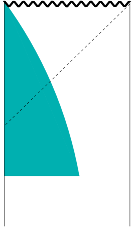
Figure 7: Collapsing ball of dust in anti de-Sitter space.

The internal metric takes Friedmann’s form

$$ds^{2}=-d\tau^{2}+a(\tau)^{2}(d\chi^{2}+A(\chi)^{2}d\Omega_{d-1}^{2})$$ (A-2)

with

$$A(\chi)=\sin(\sqrt{k}\chi)/\sqrt{k},$$ (A-3)

and $k=-1,0,1$ corresponds to open, flat and closed spatial geometries, respectively.

Due to the spherical symmetry, the Einstein equation for the metric (A-2) reduces to a single ordinary differential equation:

$${\dot{a}}^{2}+k+{a^{2}\over b^{2}}={2\kappa\rho_{0}\over d(d-1)a^{d-2}}\ .$$ (A-4)

This is solvable by quadrature,

$$\tau=\int_{a_{0}}^{a}da\left[{2\kappa\rho_{0}\over d(d-1)a^{d-2}}-k-{a^{2}\over b^{2}}\right]^{-1/2}$$ (A-5)

where $a_{0}$ is an integration constant.

Outside the ball of dust, the external metric is the solution of the vacuum equation, which by Birkhoff’s theorem is $d+1$ dimensional Schwarzschild-AdS:

$$ds^{2}=-fdt^{2}+dr^{2}/f+r^{2}d\Omega_{d-1}^{2}$$ (A-6)

with

$$f=1-m/r^{d-2}+r^{2}/b^{2}\ .$$ (A-7)

These two solutions should be matched on the world-tube of the surface of the ball. In the internal coordinates, this is given by $\chi=\chi_{0}$, and in the external coordinates by a trajectory $R(t)$. We must match the induced metric and extrinsic curvature[24]. The metric of the world-tube is

$$d\sigma^{2}=-d\tau^{2}+a^{2}(\tau)A^{2}(\chi_{0})d\Omega_{d-1}^{2}$$ (A-8)

in the internal geometry, and

$$d\sigma^{2}=-fdt^{2}+\left({dR\over dt}\right)^{2}{dt^{2}\over f}+R^{2}d\Omega_{d-1}^{2}$$ (A-9)

in the external geometry. Matching these metrics then yields

$$R(t)=a(\tau)\sin(\sqrt{k}\chi_{0})/\sqrt{k}$$ (A-10)

and

$${d\tau\over dt}=\sqrt{f^{2}(R)-\left({dR\over dt}\right)^{2}\over f}\ .$$ (A-11)

The extrinsic curvature, which is the symmetrized covariant derivative of the unit normal to the surface,

$$K_{\mu\nu}=-\frac{1}{2}(\nabla_{\mu}n_{\nu}+\nabla_{\nu}n_{\mu})\ ,$$ (A-12)

can also be computed in the internal and external geometries. In the internal geometry, we find

$$K_{\tau\tau}=0$$ (A-13)

$$K_{\theta\theta}=-a(\tau)A(\chi_{0})\frac{dA}{d\chi}\ .$$ (A-14)

In the external metric (A-6), the independent components of the extrinsic curvature are

$$K_{\tau\tau}=\frac{\ddot{R}+f^{\prime}(R)/2}{\sqrt{f+\dot{R}^{2}}}$$ (A-15)

$$K_{\theta\theta}=-R\sqrt{\dot{R}^{2}+f}\ .$$ (A-16)

where dot denotes derivative with respect to $\tau$. To the conditions (A-10), (A-11), curvature matching adds

$$\cos(\sqrt{k}\chi_{0})=\sqrt{\dot{R}^{2}+f(R)}\ .$$ (A-17)

Comparing (A-17) with the Einstein equation (A-4), we obtain the relation between the mass and the parameters of the dust configuration:

$$m={2\kappa\rho_{0}\over d(d-1)}\left[{\sin({\sqrt{k}}\chi_{0})\over{\sqrt{k}}}\right]^{d}\ .$$ (A-18)

References

- [1] S. B. Giddings, “Quantum mechanics of black holes,” Lectures given at Summer School in High Energy Physics and Cosmology, Trieste, Italy, 13 Jun - 29 Jul 1994, arXiv:hep-th/9412138.
- [2] S. B. Giddings, “The Black hole information paradox,” arXiv:hep-th/9508151.
- [3] A. Strominger, “Les Houches lectures on black holes,” arXiv:hep-th/9501071.
- [4] G. ’t Hooft, “Black Holes, Hawking Radiation, And The Information Paradox,” Nucl. Phys. Proc. Suppl. 43, 1 (1995).
- [5] G. ’t Hooft, “Dimensional Reduction in Quantum Gravity” arXiv:gr-qc/9310026.
- [6] L. Susskind, “The World as a hologram,” J. Math. Phys. 36, 6377 (1995) [arXiv:hep-th/9409089].
- [7] J. Maldacena, “The large limit of superconformal field theories and supergravity,” Adv. Theor. Math. Phys. 2, 231 (1998) [Int. J. Theor. Phys. 38, 1113 (1998)] [arXiv:hep-th/9711200].
- [8] S. S. Gubser, I. R. Klebanov and A. M. Polyakov,“Gauge theory correlators from non-critical string theory,” Phys. Lett. B 428, 105 (1998) [arXiv:hep-th/9802109].
- [9] E. Witten, “Anti-de Sitter space and holography,” Adv. Theor. Math. Phys. 2, 253 (1998) [arXiv:hep-th/9802150].
- [10] S. B. Giddings, “The boundary S-matrix and the AdS to CFT dictionary,” Phys. Rev. Lett. 83, 2707 (1999) [arXiv:hep-th/9903048].
- [11] V. Balasubramanian, S. B. Giddings and A. E. Lawrence, “What do CFTs tell us about anti-de Sitter spacetimes?,” JHEP 9903 (1999) 001 [arXiv:hep-th/9902052].
- [12] J. Polchinski, “S-matrices from AdS spacetime,” arXiv:hep-th/9901076.
- [13] L. Susskind, “Holography in the flat space limit,” arXiv:hep-th/9901079.
- [14] S. B. Giddings, “Flat-space scattering and bulk locality in the AdS/CFT correspondence,” Phys. Rev. D 61, 106008 (2000) [arXiv:hep-th/9907129].
- [15] E. Witten, “Anti-de Sitter space, thermal phase transition, and confinement in gauge theories,” Adv. Theor. Math. Phys. 2, 505 (1998) [arXiv:hep-th/9803131].
- [16] T. Banks, M. R. Douglas, G. T. Horowitz and E. J. Martinec, “AdS dynamics from conformal field theory,” arXiv:hep-th/9808016.
- [17] V. Balasubramanian, P. Kraus, A. E. Lawrence and S. P. Trivedi, “Holographic probes of anti-de Sitter space-times,” Phys. Rev. D 59, 104021 (1999) [arXiv:hep-th/9808017].
- [18] I. Chepelev and R. Roiban, “A note on correlation functions in AdS(5)/SYM(4) correspondence on the Coulomb branch,” Phys. Lett. B 462, 74 (1999) [arXiv:hep-th/9906224].
- [19] S. B. Giddings and S. F. Ross, “D3-brane shells to black branes on the Coulomb branch,” Phys. Rev. D 61, 024036 (2000) [arXiv:hep-th/9907204].
- [20] J. M. Maldacena, “Eternal black holes in Anti-de-Sitter,” arXiv:hep-th/0106112.
- [21] R. Gregory and R. Laflamme, “Black strings and p-branes are unstable,” Phys. Rev. Lett. 70, 2837 (1993) [arXiv:hep-th/9301052].
- [22] U. H. Danielsson, E. Keski-Vakkuri and M. Kruczenski, “Spherically collapsing matter in AdS, holography, and shellons,” Nucl. Phys. B 563, 279 (1999) [hep-th/9905227].
- [23] U. H. Danielsson, E. Keski-Vakkuri and M. Kruczenski, “Black hole formation in AdS and thermalization on the boundary,” JHEP 0002, 039 (2000) [hep-th/9912209].
- [24] W. Israel, “Singular Hypersurfaces And Thin Shells In General Relativity,” Nuovo Cim. B 44S10, 1 (1966) [Erratum-ibid. B 48, 463 (1966)].
- [25] K. Kuchar “Charged shells in general relativity and their gravitational collapse.” Czech. J. Phys B 18, 435 (1968)
- [26] G. T. Horowitz and N. Itzhaki, “Black holes, shock waves, and causality in the AdS/CFT correspondence,” JHEP 9902, 010 (1999) [arXiv:hep-th/9901012].
- [27] W. G. Unruh, “Notes On Black Hole Evaporation,” Phys. Rev. D 14, 870 (1976).
- [28] G. W. Gibbons and M. J. Perry, “Black Holes And Thermal Green’s Functions,” Proc. Roy. Soc. Lond. A 358, 467 (1978).
- [29] J. B. Hartle and S. W. Hawking, “Path Integral Derivation Of Black Hole Radiance,” Phys. Rev. D 13, 2188 (1976).
- [30] T. Jacobson, “A Note on Hartle-Hawking vacua,” Phys. Rev. D 50, 6031 (1994) [arXiv:gr-qc/9407022].
- [31] T. A. Jacobson, “Introduction to Black Hole Microscopy,” arXiv:hep-th/9510026.
- [32] W. Israel, “Thermo Field Dynamics Of Black Holes,” Phys. Lett. A 57, 107 (1976).
- [33] P. Candelas, “Vacuum Polarization In Schwarzschild Space-Time,” Phys. Rev. D 21, 2185 (1980).
- [34] S. Mukohyama and W. Israel, “Black holes, brick walls and the Boulware state,” Phys. Rev. D 58, 104005 (1998) [arXiv:gr-qc/9806012].
- [35] P. C. Davies and S. A. Fulling, “Radiation From A Moving Mirror In Two-Dimensional Space-Time Conformal Anomaly,” Proc. Roy. Soc. Lond. A 348, 393 (1976).
- [36] K. Melnikov and M. Weinstein, “A canonical Hamiltonian derivation of Hawking radiation,” arXiv:hep-th/0109201.
- [37] S. S. Gubser, I. R. Klebanov and A. W. Peet, “Entropy and Temperature of Black 3-Branes,” Phys. Rev. D 54, 3915 (1996) [arXiv:hep-th/9602135].
- [38] S. W. Hawking, “Particle Creation By Black Holes,” Commun. Math. Phys. 43, 199 (1975).
- [39] A. Ilha and J. P. Lemos, “Dimensionally continued Oppenheimer-Snyder gravitational collapse. I: Solutions in even dimensions,” Phys. Rev. D 55, 1788 (1997) [arXiv:gr-qc/9608004].
- [40] J. P. Lemos, “Collapsing shells of radiation in anti-de Sitter spacetimes and the hoop and cosmic censorship conjectures,” Phys. Rev. D 59, 044020 (1999) [arXiv:gr-qc/9812078].
- [41] A. Ilha, A. Kleber and J. P. Lemos, “Dimensionally continued Oppenheimer-Snyder gravitational collapse. II: Solutions in odd dimensions,” J. Math. Phys. 40, 3509 (1999) [arXiv:gr-qc/9902054].