Finite-Temperature Gluon Condensate with
Renormalization Group Flow Equations

Abstract

Within a self-consistent proper-time Renormalization Group (RG) approach we investigate an effective QCD trace anomaly realization with dilatons and determine the finite-temperature behavior of the gluon condensate. Fixing the effective model at vanishing temperature to the glueball mass and the bag constant a possible gluonic phase transition is explored in detail. Within the RG framework the full non-truncated dilaton potential analysis is compared with a truncated potential version.

PACS: 05.10.Cc, 64.60.A, 14.70.D

1 Introduction

Perturbative QCD studies and lattice simulations demonstrate that the fundamental quark and gluon degrees of freedom are the relevant ones at high temperatures. Since these degrees of freedom are confined in the low-temperature regime there must be a quark and/or gluon deconfinement phase transition at high temperature.

Difficulties arise in the description of this phase transition due to the absence of local parameters which can be linked to confinement. QCD at low energies can be approximated by effective models which have to satisfy the observed symmetry properties and anomaly structure of the theory. Besides the important approximate and spontaneously broken chiral symmetry at low energy, the classical QCD-Lagrangian exhibits an additional dilatation symmetry or scale invariance in the limit of vanishing current quark masses which is embedded in a larger conformal group. This symmetry is broken at the quantum level by radiative corrections – the so-called trace anomaly.

In order to mimic the trace anomaly in an effective framework one introduces a scalar ($J^{PC}=0^{++}$) dilaton field $\chi$ with scaling dimension one and a logarithmic potential with coupling $h$ of the form [1, 2]

$$V = h\left(\frac{\chi}{\chi_{0}}\right)^{4}\ln\left(\frac{\chi}{\chi_{0}e^{1/4}}\right)\ .$$ (1)

This potential breaks scale invariance and leads therefore to a finite vacuum expectation value (VEV) $\chi_{0}\equiv\langle 0|\chi|0\rangle$. In this way the anomalous breaking of scale invariance is effectively taken into account. This can be seen by identifying the trace of the energy-momentum tensor, $\theta_{\mu}^{\mu\ \mbox{\scriptsize eff}}$, of the effective theory with the trace of the modified (symmetric) energy-momentum tensor $\theta_{\mu}^{\mu\ \mbox{\scriptsize QCD}}$ of massless QCD. The trace is related to the divergence of the dilatation current $J_{\mu}^{\mbox{\scriptsize dil}}$, which vanishes at tree level where fluctuations are omitted:

$$\partial^{\mu}J_{\mu}^{\mbox{\scriptsize dil}}=-\frac{h}{\chi_{0}^{4}}\chi^{4}=\theta_{\mu}^{\mu\ \mbox{\scriptsize eff}} \stackrel{{\scriptstyle!}}{{=}} \theta_{\mu}^{\mu\ \mbox{\scriptsize QCD}}=\frac{\beta(g)^{\mbox{{\scriptsize QCD}}}}{2g}G_{\mu\nu}G^{\mu\nu}\ .$$ (2)

Here $G_{\mu\nu}$ denotes the non-Abelian field strength tensor, $\beta(g)^{\mbox{{\scriptsize QCD}}}$ the QCD beta (Gell-Mann–Low) function and $g$ is the gauge coupling.

Beyond tree level, however, massless QCD is no longer scale-invariant. Due to the renormalization, a new dimensionful cut-off hidden in the QCD beta function must be introduced. Despite this fact, the anomaly does not depend on the chosen regularization scheme. The effective realization of the trace anomaly can be achieved by equating the divergence of the dilatation current with the dilaton field. This yields a differential equation for the $a$ $priori$ unknown effective dilaton potential whose solution is Eq. (1).

This effective realization allows for an identification of the gluon condensate $\langle 0|G_{\mu\nu}G^{\mu\nu}|0\rangle$ with the VEV $\chi_{0}$ of the effective theory with broken scale invariance via Eq. (2). Following the suggestion of Campbell et al. [3] $\chi_{0}$ can be regarded as an effective order parameter for the deconfining phase transition. The authors find a strong correlation with the chiral phase transition, arguing that a first-order gluonic phase transition might drive the usual second-order chiral phase transition for two flavors, thereby changing it to first order. Their conclusion is that the quark condensation temperature, $T_{q}$, for the chiral phase transition is always smaller or equal to the gluon condensation or confinement temperature $T_{g}$. Even for large $N_{c}$ and fixed number of flavours the quark transition would be driven by the gluon transition, because $T_{q}$ and $T_{g}$ coincide in this case with the critical temperature of a first-order gluon transition.

In order to investigate these findings we perform a finite-temperature analysis of the effective theory within the framework of a proper-time renormalization group (PTRG) approach. With the logarithmic interaction potential in Eq. (1) the Lagrangian becomes non-renormalizable. One possible regularization of the infinite $T=0$ contributions would be the introduction of a cut-off parameter $\Lambda$ which determines the scale up to which the effective description of the theory is valid, similar to a model parameterization of the Nambu–Jona-Lasinio type. Such a new dimensionful cut-off would violate the scaling properties of the effective theory. In order to maintain the desired scaling behavior, one has to give the cut-off-parameter a conformal weight of unit one by some mechanism.

For the purely gluonic Lagrangian specified by the potential in Eq. (1), a direct comparison of the free energy or effective potential at the origin, and at the local minimum, needed in a perturbative approach, is not possible due to the breakdown of the Taylor expansion of the potential itself. It is therefore impossible to determine perturbatively the order (first or second) of the phase transition signalled by the disappearance of the scalar dilaton field $\chi_{0}$ as the order parameter.

In order to address the question of the order of the gluon phase transition, Campbell et al. [3] introduced an additional term proportional to $\chi^{n}$ ($n<4$) to the effective potential in Eq. (1) with an $a$ $priori$ unknown temperature-dependent coefficient. They chose phenomenologically a monotonically increasing function of temperature for this coefficient. Neglecting effects of order ${\cal O}(T^{4})$ in the finite-temperature contributions to the effective potential, a first-order transition was found, as one would expect from lattice simulations [4].

Within the PTRG approach we can circumvent these difficulties by directly calculating the full non-truncated effective dilaton potential for any value of the field and not just at the minimum, $\chi_{0}$. This in principle allows to analyze the order of the phase transition.

The outline of the paper is as follows: In Sec. 2 we introduce a self-consistent RG method combined with a Schwinger (proper-time) regularization. We derive flow equations for two different scenarios. The dilaton model is discussed without any polynomial potential truncation in Sec. 3. This full potential calculation is compared to an analysis in a truncated potential approximation, followed by an error estimation in Sec. 4. Finally, in Sec. 5 we present our conclusions.

2 The Renormalization Group approach

The RG approach used in the present work is based on a perturbative one-loop expression for the effective potential, which is regularized by Schwinger’s proper-time representation of the divergent logarithm. The usual Schwinger proper-time integral is modified by a regulator or blocking function $f_{k}$ in the integrand, thus rendering the resulting flow equation infrared (IR) and ultraviolet (UV) finite. In this way the IR flow scale $k$ is introduced [5, 6]. The flow equation that describes the scale dependence of the action $\Gamma_{k}$ reads

$$k\frac{\partial\Gamma_{k}}{\partial k} = -\frac{1}{2}\int\limits_{0}^{\infty}\frac{d\tau}{\tau}\left(k\frac{\partial f_{k}}{\partial k}\right)\mbox{Tr}\;e^{\displaystyle-\tau\Gamma^{(2)}_{k}}$$ (3)

where on the $rhs$ a renormalization group improvement is performed by a replacement of the bare second derivative of the action w.r.t. the fields with the corresponding running expression $\Gamma^{(2)}_{k}$ [8]. This replacement improves the one-loop flow equation and corresponds to a resummation of higher Feynman graphs i.e. daisy and superdaisy diagrams [6, 9], similar to a Schwinger-Dyson resummation. In a plane-wave basis the blocking function $f_{k}$ serves as a momentum regulator similar to the regulator $R_{k}$ in the ’Exact Renormalization Group’ (ERG) [10] and selects only modes which are peaked around the scale $k$ [11]. The direct connection to the cut-off $R_{k}$ in the ERG formalism is still missing but the issue whether this proper-time flow converges to the full effective action will not be discussed here. We also omit a detailed analysis of the scheme dependence introduced by the choice of the regulator function [11, 12].

The regulator has to fulfil basically two conditions: The modified action $\Gamma_{k}$ should tend to the full action in the IR limit, requiring that $f_{k\to 0}(\tau\to\infty)\to 1$. In this way the cut-off is removed and all quantum fluctuations are taken into account. In addition we have to set $f_{k}(\tau=0)=1$ for arbitrary $k$. This does not regularize the UV regime ($\tau=0$) which is not necessary anyway if we start the evolution at a finite (large) UV scale $\Lambda$. Finally, for the derivation of all flow equations we will employ the following choice for the blocking function $f_{k}$ in $d$ space-time dimensions:

$$k\frac{\partial f_{k}}{\partial k} = -\frac{4}{d\Gamma(d/2)}(\tau k^{2})^{d/2+1}e^{-\tau k^{2}}$$ (4)

corresponding to the notation $f_{k}^{(1)}$ in [8].

Of course, it is not possible to solve the full RG equation (3) without truncation. In order to obtain a tractable set of coupled flow equations we perform a derivative expansion of the effective action which takes the generic form

$$\Gamma_{k}[\phi] = \int d^{d}x\left\{V_{k}(\phi)+\frac{1}{2}Z_{k}(\phi)(\partial_{\mu}\phi)^{2}+\ldots\right\}\ .$$ (5)

In this work we consider the local potential approximation (LPA) in which the running of the wavefunction renormalization $Z_{k}$ is neglected ($Z_{k}$ is set to unity) and only the effective potential $V_{k}$ is taken into account.

The task is to solve the resulting coupled non-linear flow equation for the potential $V_{k}$ by starting in the ultraviolet with $a$ $priori$ unknown initial conditions and integrate towards zero momentum with respect to the scale $k$. In this way all quantum fluctuations are effectively taken into account. The initial conditions at the UV scale are determined in such a way that calculated physical quantities in the IR are matched to predetermined values.

The generalization of our RG method to finite temperature within the Matsubara formalism is straightforward. Details can be found in Refs. [8, 13, 14]. In the zero-momentum components of the loop integration of Eq. (3) one has to introduce bosonic Matsubara frequencies $\omega_{n}=2\pi nT$. In the LPA the resulting momentum integrals can be performed analytically, leading to fractional powers in the finite-temperature threshold functions and hence to the dimensional reduction phenomenon [14, 15].

3 The full dilaton potential

The aim of the next two sections is to derive and solve numerically flow equations for the gluon condensate from an effective dilaton Lagrangian with a logarithmic interaction potential. In this section we consider the full dilaton interaction potential without any polynomial potential truncation and will compare the results with a truncated potential calculation in the next section.

As motivated in the introduction we start with the following effective Lagrangian in Euclidean space

$${\cal L} = \frac{1}{2}(\partial_{\mu}\chi)^{2}+V_{0}(\chi)\qquad\mbox{with}\qquad V_{0}(\chi)=h\left(\frac{\chi}{\chi_{0}}\right)^{4}\ln\left(\frac{\chi}{\chi_{0}e^{1/4}}\right)\ .$$ (6)

The potential $V_{0}$ is parameterized by two constants. The depth is determined by the coupling $h$ and the curvature is given by the minimum $\chi_{0}$. The minimum is asymmetric and small oscillations about $\chi_{0}$ can be interpreted as a massive scalar gluonium (glueball) state. Difficulties arise around $\chi=0$ since the potential is unstable (actually not defined as mentioned in the introduction). Therefore, a particle interpretation at the origin is also no longer possible. For Campbell et al. [3] this phenomenon is an indication that glueballs are no longer the relevant degrees of freedom at that point. All physical hadrons (if there is any phase transition in the effective model) are dissolved into their perturbative gluon content and this phase corresponds to a deconfined phase.

At the minimum $\chi_{0}$ the potential is equal to $V_{0}(\chi_{0})=-h/4$. This allows for an identification of the coupling $h$ with the bag constant $B$ which is the negative of the energy density of the vacuum $\epsilon_{vac}$ via the relation

$$B=V_{0}(0)-V_{0}(\chi_{0}) = -\epsilon_{vac}=\frac{h}{4}\ .$$ (7)

Since we are able to calculate the potential at the origin, this relation can be used to determine $B$ in the IR.

The first derivative of the potential w.r.t. the scalar field $\chi$, denoted in the following with a prime, $V_{0}^{\prime}\equiv dV_{0}/d\chi$, vanishes when evaluated at the minimum. The second derivative $V_{0}^{\prime\prime}(\chi_{0})=4h/\chi_{0}^{2}=m^{2}_{\chi}$ yields the tree-level glueball squared mass, $m^{2}_{\chi}$. In this work the glueball mass is taken as an input. We choose values around $m_{\chi}=1.5$ GeV which is motivated by recent lattice results [16]. The experimental situation is not clear up to now but glueball candidates in the mass region of $1.5\ldots 1.8$ GeV are favored [17]. For instance, a possible candidate could be the $f_{0}(1500)$ meson. The value of the bag constant $B$ which serves as a second input is not well known but ranges between $B^{1/4}=0.14\ldots 0.24$ GeV. Thus, using e.g. $B^{1/4}=0.24$ GeV and $m_{\chi}^{2}=1.5^{2}$ GeV² at the UV scale (tree level) yields $h^{1/4}=0.34$ GeV and $\chi_{0}=0.154$ GeV. In Ref. [18] it is observed that the temperature scale, where thermal excitations become important, is determined by the value of the bag constant at $T=0$. For $B^{1/4}=0.14$ GeV, the onset of a significant shift of the minimum is seen at $T\sim 0.25$ GeV while for $B^{1/4}=0.24$ GeV this happens only for temperatures above $T\sim 0.4$ GeV. In fact, it was found in [18] that the value for the “critical” temperature $T_{c}$ is dominated by the value of the bag constant. A larger bag constant results in a higher critical temperature, although the authors cannot determine a real first- or second-order phase transition. From the difference between the RG evolved potential in the IR at the true minimum $\chi_{0}$ and the potential at the origin we can calculate the bag constant by means of Eq. (7) and find a similar dependence of the “critical” temperature on the bag constant.

In order to investigate the behavior of the dilatons in a RG picture we apply the method presented in Sec. 2 to the Lagrangian of Eq. (6). For the dilaton potential in the LPA with $d$ Euclidean space-time dimensions and the smearing function $f^{(1)}_{k}$ we obtain the following flow equation:

$$\partial_{t}V_{k} = \frac{2}{(4\pi)^{d/2}\Gamma(d/2)}\frac{k^{d}}{d}\frac{1}{(1+\tilde{V_{k}}^{\prime\prime})}\ ,$$ (8)

where $t=\ln(k/\Lambda)$ and the tilde indicates the rescaled quantity w.r.t. the IR squared scale $k^{2}$, e.g. $\tilde{V}^{\prime\prime}_{k}=V^{\prime\prime}_{k}/k^{2}$. In order to solve this coupled equation we discretize the field $\chi$ for a general potential $V(\chi)$ on a grid. To close the system of equations we need to derive an equation for the first derivative $V^{\prime}_{k}$ [19]. This generates higher derivatives of the potential on the $rhs$ of Eq. (8) up to $V^{\prime\prime\prime}_{k}$. These higher derivatives are then numerically determined by matching conditions, based on a Taylor-expansion of $V_{k}$ and $V^{\prime}_{k}$ at intermediate grid points. In this way we obtain a highly coupled closed system of flow equations which can be solved numerically with a 5th order Cash-Karp Runge-Kutta method [20]. The advantage of closing the system in this way is that we do not need higher than third-order derivatives. Since the expansion of a logarithmic potential at the origin in a power series leads to singular coefficients for powers larger than three this signals the breakdown of a perturbative treatment of the model, as already mentioned in the introduction. Via the application of the non-perturbative RG method we can circumvent these singularities.

The initial conditions for the coupling $h$ and minimum $\chi_{0}$ are determined at the UV scale $\Lambda$ by fits to the glueball mass $m^{2}_{\chi}$ and the bag constant $B$ at the end of the evolution in the IR. We have chosen $\Lambda=2.0$ GeV, $\chi_{0}=0.137$ GeV and a coupling $h=(0.51\mbox{GeV})^{4}$ and start with a logarithmic dilaton potential (tree level). These initial values result after the $k$-evolution in a bag value of $B^{1/4}=0.276$ GeV and a glueball ball mass of $m_{\chi}=1.502$ GeV.

Figure 1: The $k$-evolution of the potential $V_{k}$ (left panel) versus $\chi$ and the $k$-evolution of the normalized minimum $\chi_{0}(k)/\chi_{0}(k=0)$ versus $k$ (right panel). (h^1/4 = 0.51 GeV, $\Lambda=2.0$ GeV , $\chi_{0}(\Lambda)=0.137$ GeV).

Due to the radiative corrections (quantum fluctuations) the shape of the effective logarithmic potential is altered when evolving towards the IR as shown in Fig. 1 (left panel). In the IR, the potential becomes convex for all $\chi$ values. This is consistent with the definition of the scale anomaly.

The structure of the threshold functions in the flow Eqs. (8) is very similar to those for the $O(N)$ symmetric model [8]. Due to a negative curvature of the potential for small $\chi$ which is typical for broken symmetries, poles can occur in the threshold functions. For instance, $V^{\prime\prime}_{k}/k^{2}$ starts with negative values for small field amplitudes $\chi$ during the $k$-evolution. That is the reason why there is a correlation of the initial values $h$, $\chi_{0}$ and the UV scale $\Lambda$ and why they cannot be chosen independently. To avoid a pole in the threshold function we have to choose initial values in such a way that $V^{\prime\prime}_{k}/\Lambda^{2}$ is larger than -1 and $V^{\prime\prime}_{k}$ becomes positive for all field amplitudes $\chi$ during the evolution towards the IR. In the right panel of Fig. 1 the $k$-evolution of the normalized minimum is presented. One recognizes that the evolution almost stops around $k\approx 0.4$ GeV.

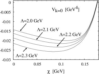
Figure 2: The evolved effective potential $V_{k=0}$ versus $\chi$ for various values of the UV cutoff $\Lambda$ (h^1/4 = 0.51 GeV, $\chi_{0}(\Lambda)=0.137$ GeV).

In order to estimate the theoretical uncertainty of these results we show in Fig. 2 the UV cutoff dependence of the evolved effective potential $V_{k=0}$ for values $\Lambda=2.0-2.3$ GeV at fixed coupling $h^{1/4}=0.51$ GeV and a fixed minimum $\chi_{0}=0.137$ GeV.

$\qquad\Lambda\quad\mbox{{[GeV]}}$	$\qquad B^{1/4}\quad\mbox{{[GeV]}}$	$\qquad m_{\chi}\quad\mbox{{[GeV]}}$
2.0	0.276	1.502
2.1	0.270	1.409
2.2	0.264	1.356
2.3	0.258	1.337

Table 1: UV cutoff dependence of the bag constant $B$ and glueball mass $m_{\chi}$. See text for details.

The evolved minimum $\chi_{0}$ of the potential is shifted towards smaller values for higher UV cutoffs. Due to the longer evolution with increasing UV cutoff the absolute depth of the potential is also increasing. Nevertheless the change for the bag constant is small (cf. Tab. 3) because, for its calculation via Eq. (7), only the potential difference enters. In Tab. 3 the cutoff dependence of the glueball mass $m_{\chi}$ is also listed. The decrease of the glueball mass with increasing UV cutoff is more sensitive.

On the other hand if we keep the UV cutoff $\Lambda$ fixed and vary the coupling $h$ or the minimum $\chi_{0}$ at the initial UV scale we obtain in both cases a rather weak depencence of $B$ and $m_{\chi}$. The glueball mass and the bag constant decrease with decreasing $h$. The variation of $\chi_{0}$ is anyway restricted to a small interval (within 7 % of $\chi_{0}$) in order to avoid a pole in the threshold function already mentioned above. Within this interval the glueball mass decreases within 2% while the bag constant increases within 2 % for increasing $\chi_{0}$.

3.1 Finite-temperature evolution

Within the Matsubara formalism, the finite-temperature version of the self-consistent flow Eq. (8) is given by the following expression [8, 14]

$$\partial_{t}V_{k}(\chi) = \frac{2\;\;\Gamma(3/2)}{{(4\pi)^{(d-1)/2}}\Gamma(d/2)}\frac{k^{d-1}}{d}T\!\!\sum\limits_{n=-\infty}^{\infty}\frac{1}{(1+\tilde{\omega}^{2}_{n}+\tilde{V}^{\prime\prime}_{k})^{3/2}}\ .$$ (9)

The non-integer powers in the threshold functions are typical for the finite-temperature version within this approach and are governed by the choice of the smearing functions $f_{k}$. At finite temperature we again solve, analogous to the zero-temperature case, the flow equation (9) numerically by discretizing the $\chi$ field. We use the same zero-temperature initial conditions at the UV scale $\Lambda=2.0$ GeV. Note that this choice restricts the finite-temperature predictions of our results for higher temperatures. The predictive power of the finite-temperature extrapolation is basically determined by the structure of the threshold functions in the flow equations and the value of the UV cut-off. A detailed discussion can be found in Ref. [14]. With $\Lambda=2.0$ GeV we can ignore the temperature dependence of the initial values at the UV scale up to temperatures around $T\sim 250$ MeV.

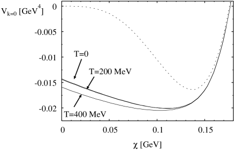
Figure 3: The potential $V_{k=0}$ (h^1/4 = 0.51 GeV, $\Lambda=2.0$ GeV , $\chi_{0}=0.137$ GeV ) versus the $\chi$ field for different temperatures ($\Delta T=200$ MeV, see text for details).

In Fig. 3 we show the temperature behavior of the potential in the IR. The dashed curve corresponds to the initial bare potential at $k=\Lambda$. After the $k$ evolution we obtain the solid curve, labeled by $T=0$ MeV, corresponding to the zero temperature IR potential. We repeat this procedure in steps of $200$ MeV. Below temperatures of the order of $200$ MeV no significant changes in the potential shape are observed.

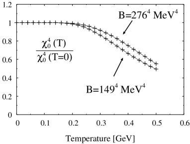
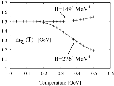
Figure 4: The temperature-dependent normalized minimum $\chi_{0}^{4}(T)/\chi_{0}^{4}(T=0)$ of the potential (left panel) and the glueball mass $m_{\chi}$ (right panel) for two different bag constants (see text for details).

In analogy to the restoration of spontaneously broken chiral symmetry at high temperature, we regard the temperature-dependent minimum of the dilaton potential as an order parameter for the deconfining phase transition under the assumption of factorization (see [3]). Deconfinement would thus be signalled by a transition from a finite VEV $\chi_{0}\neq 0$ to a vanishing one $\chi_{0}=0$.

We observe a change of the normalized ’order parameter’ $\chi_{0}^{4}(T)/\chi_{0}^{4}(0)$ with temperature as shown in the left panel of Fig. 4 for two different values of the bag constant $B$ but equal glueball mass $m_{\chi}=1.5$ GeV in the IR. For both bag constants the condensate stays almost constant up to temperatures of the order $200$ MeV which is beyond the chiral phase transition temperature for two quark flavors [4]. For the smaller bag constant $B^{1/4}=0.149$ GeV, which we obtain for $h^{1/4}=0.34$ GeV and $\chi_{0}=0.068$ GeV at the UV scale $\Lambda=2.0$ GeV, the condensate starts to decrease earlier. Thus, we can qualitatively verify the dependence of the “critical temperature” on the bag constant. In contrast to Ref. [18] the onset of the shift in the condensate is seen earlier at $T\sim 190$ MeV. It then decreases almost linearly in both cases. The negative slope for temperatures beyond $300$ MeV does not depend on the chosen value for the bag constant. At these temperatures we lose, however, predictive power due to the omission of the temperature dependence of the initial values at the UV scale (see also Ref. [14]). In the right panel the temperature-dependent glueball mass $m_{\chi}$ is displayed for two different bag constants. The mass as function of temperature is independent on the bag constant below temperatures of $180$ MeV. For the larger bag constant $B^{1/4}=0.276$ GeV it then decreases but increases again for very large temperatures above $800$ MeV. For the smaller bag constant $B^{1/4}=0.149$ GeV the mass grows almost linearly with temperature around $T\sim 350$ MeV. At very high temperatures such a behavior is expected since perturbation theory is applicable (cf. [26]). It turns out that this behavior is almost independent of the initial $\Lambda,$ at least for temperatures below $250$ MeV.

If we vary the cut-off $\Lambda$ between 1.5 and 2 GeV, while tuning the coupling $h$ and $\chi_{0}$ to keep the glueball mass and the bag constant fixed, we do not observe any significant changes below temperatures of $200$ MeV.

Another more general way to find a possible RG fixed point solution from a continuous flow equation starts with the rescaled fixed point flow equation [21]. For this purpose we introduce a dimensionless potential $U(\bar{\chi})=(4\pi)^{2}k^{-4}V_{k}(\chi)$ and field $\bar{\chi}=(4\pi)k^{-1}\chi$ in Eq. (8) and set $\partial_{t}U=0$ which defines the fixed point. In the LPA and $d=4$ this yields the flow equation

$$4U(\bar{\chi})-\bar{\chi}U^{\prime}(\bar{\chi}) = \frac{1}{2}\frac{1}{(1+U^{\prime\prime}(\bar{\chi}))}\ .$$ (10)

This equation has a continuum of solutions which depends on the initial boundary conditions. For the solution we have to specify two boundary conditions. One is fixed by the necessary equation $U^{\prime}(0)=0$ at the critical point. If we choose some value for $U(0)$ we can now numerically integrate Eq. (10) out to positive fields $\chi$. We almost always find a singularity at some critical field $\chi=\chi_{c}$ where the numerics breaks down. The result is depicted in Fig. 5 where we find two exceptions. The first peak at $U(0)=0$ corresponds to a singular solution where $U^{\prime\prime}(0)$ diverges. Only for the second peak at $U(0)=1/8$ the potential seems to exist for all fields $\chi$. At this point the second derivative vanishes and the potential itself is non-singular and constant (trivial) for all fields $\chi$.

Figure 5: The singularity $\chi_{c}$ as function of $U(0)$.

The peaks are generated by the threshold functions in Eq. (10) and therefore depend on the choice of the smearing function. The second solution is exactly at $U(0)=1/8$ for a smearing function $f_{k}^{(m)}$ of the first kind $m=1$ [8]. Higher smearing functions will influence the overall factor of the flow equations moving the second peak towards zero like $2/(m+1)!$ [12]. We conclude that no further non-trivial non-singular fixed point arises within the LPA. A similar analysis for three space-time dimensions is omited here since the extrapolation and implementation of the anomaly is far from trivial.

4 The truncated dilaton potential

In the previous section we have solved the non-truncated flow equation (8) for the full dilaton potential in the LPA by discretizing the scalar field $\chi$ on a grid. Alternatively, one can expand the potential in a Taylor series around the non-vanishing local minimum $\chi_{0}$ (or any other field value) and derive flow equations for the (in principle infinitely many) expansion coefficients [22]. This allows for a direct study of the flow of the coupling constants. We will investigate this procedure in this section. Due to the termination of the potential series at a finite power we expect new truncation effects. At any given finite order of truncation there are always higher-order operators which do not evolve and could thus influence the accuracy of the solutions. In the limit of infinitely many expansion coefficients we should, of course, reproduce all results from the previous section.

The non-invariant Taylor expansion around the scale-dependent minimum $\chi_{0}$ (broken phase) up to a specific order $M$ is given by

$$V_{k}(\chi) = c_{0}(k)+\sum\limits_{n=2}^{M}\frac{c_{n}(k)}{n!}(\chi-\chi_{0}(k))^{n}\ .$$ (11)

In the LPA the expansion coefficients, $c_{n}$, defined at the minimum $\chi_{0}$, correspond to the $n$-point proper vertices evaluated at zero momenta [23]. Substituting the potential expansion on both sides of Eq. (8) we can deduce a set of coupled flow equations for the first several couplings $c_{n},\ n=0,2,3,\ldots$.

$$\dot{c}_{0} = \frac{1}{2(4\pi)^{2}}\frac{k^{4}}{1+c_{2}/k^{2}}$$

$$\dot{c}_{1} = c_{2}\dot{\chi}_{0}+\dot{c}_{0}\left[-\frac{G_{3}}{k^{2}}\right]=0$$ (12)

$$\dot{c}_{2} = c_{3}\dot{\chi}_{0}+\dot{c}_{0}\left[\frac{2G_{3}^{2}}{k^{4}}-\frac{G_{4}}{k^{2}}\right]$$

$$\dot{c}_{3} = c_{4}\dot{\chi}_{0}+\dot{c}_{0}\left[-6\frac{G_{3}^{3}}{k^{6}}+6\frac{G_{3}G_{4}}{k^{4}}-\frac{G_{5}}{k^{2}}\right]$$

$$\dot{c}_{4} = c_{5}\dot{\chi}_{0}+\dot{c}_{0}\left[9\frac{G_{3}^{4}}{k^{8}}-36\frac{G_{3}^{2}G_{4}}{k^{6}}+8\frac{G_{3}G_{5}}{k^{4}}+6\frac{G_{4}^{2}}{k^{4}}-\frac{G_{6}}{k^{2}}\right]$$

$$\dot{c}_{5} = c_{6}\dot{\chi}_{0}+\dot{c}_{0}\left[-120\frac{G_{3}^{5}}{k^{10}}+240\frac{G_{3}^{3}G_{4}}{k^{8}}-60\frac{G_{3}^{2}G_{5}}{k^{6}}-90\frac{G_{3}G_{4}^{2}}{k^{6}}+\right.$$

$$\vdots \qquad\qquad\qquad\qquad\qquad\qquad\qquad\left.+10\frac{G_{3}G_{6}}{k^{4}}+20\frac{G_{4}G_{5}}{k^{4}}-\frac{G_{7}}{k^{2}}\right]$$

with the definition $G_{n}\equiv\frac{\displaystyle c_{n}}{\displaystyle(1+c_{2}/k^{2})}$. The corresponding $\beta_{n}$-functions, $\beta_{n}\equiv k\frac{\displaystyle\partial c_{n}}{\displaystyle\partial k}=\partial_{t}c_{n}\equiv\dot{c}_{n}$, depend on $\beta_{n}=\beta_{n}(c_{0},c_{1},\ldots,c_{n+2})$ for all $n$. Due to the absence of a reflection symmetry ($Z_{2}$ symmetry) we realize that all odd and even vertices contribute to the $\beta_{n}$-functions. The expression for $G_{n}$ can be interpreted as a generalized $n$-point vertex multiplied by a rescaled bosonic propagator with the squared dilaton self-energy, $c_{2}$, given at vanishing external momenta (cf. [13]). This interpretation exemplifies the one-loop contributions to the $\beta_{n}$-functions in a transparent and obvious scheme. For instance, the first few contributions in the brackets can be visualized diagrammatically as

Figure 6: Diagrammatical contributions to the first several $\beta_{n}$-functions.

One recognizes the one-loop structure. In the diagrams we have always omitted the first term on the $rhs$ of the $\beta_{n}$-functions which is generically depicted in Fig. 7.

Figure 7: The term $c_{n}\dot{\chi}_{0}$ which has $(n-1)$ legs.

The coefficient $c_{1}$ defines the minimum $\chi_{0}$ of the potential and always vanishes:

$$\left.V_{k}^{\prime}\right|_{\chi_{0}}=c_{1}\stackrel{{\scriptstyle!}}{{=}}0\ .$$ (13)

We have solved the coupled flow equations (4) numerically with a 5th-order Cash-Karp Runge-Kutta method for different truncation orders $M$ in order to investigate higher coupling effects in detail. As an example, in Fig. 8, the $k$-evolution of the first coefficients $-c_{0}^{1/4}$, $c_{3}$, $c_{4}$, the minimum $\chi_{0}$ and the dilaton mass $m_{\chi}=\sqrt{c_{2}}$ are shown for $M=5$. One observes that the $k$-evolution stops for all dimensionful quantities around the scale $k\approx 400$ MeV. All coefficients converge to finite IR values.

Figure 8: The scale evolution for the coefficients $-c_{0}^{1/4}$, $m_{\chi}=c_{2}^{1/2}$, $c_{3}$, $c_{4}$ and the minimum $\chi_{0}$.

In order to estimate the truncation effects we compare the truncated potential calculation for different truncation orders $M$. It turns out that in the truncated potential calculation we cannot choose the same initial values as for the full one in the previous sections. With the values $\Lambda=2$ GeV, $h^{1/4}=0.69$ GeV and $\chi_{0}=0.6$ GeV we can indeed perform the truncated potential calculation up to the order $M=9$ where we have arbitrarily stopped our truncation order. The results are presented in Fig. 9. Each curve depicts the evolved truncated potential in the IR up to a given order $M$. Due to a slightly different evolution of the minimum $\chi_{0}$ for different orders $M$ all potential curves are plotted versus the $\chi$-field normalized in the IR.

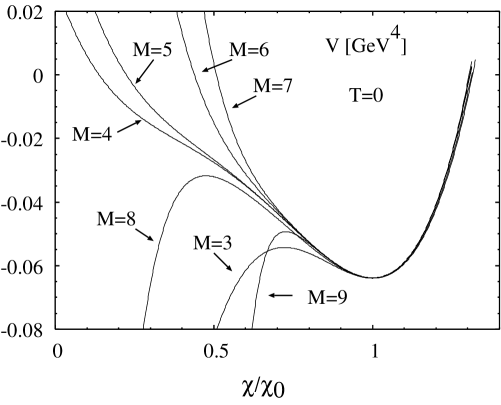
Figure 9: A comparison of the zero-temperature truncated potential calculation for different expansion order $M$, demonstrating the influence of higher operators to the potential. Each curve is labeled by the corresponding expansion order $M$.

We do not observe an improved convergence of the truncated potential to the full potential when increasing the order of the expansion. Obviously, the truncation order $M=3$ is inappropriate.

Figure 10: The glueball mass $m_{\chi}$ as function of the order, $M$, of the polynomial expansion.

In Fig. 10 the evolved IR glueball mass, $m_{\chi}$, is shown for different truncation orders $M$. All masses are obtained by the same initial values thus displaying the influence of higher operators on the mass evolution. We again do not see a convergence up to the order $M=9$.

The finite-temperature generalization of the expansion procedure is straightforward. In Fig. 11 we show the normalized minimum of the truncated potential at finite temperature for different values of $M$.

For all orders the minimum stays constant up to temperatures around $200$ MeV. For higher temperatures we see truncation effects due to the omission of higher operators in the corresponding beta-functions. The rapid temperature decrease of the minimum for truncation order $M=3$ could also be related to the smaller zero-temperature glueball mass at this order. Increasing the expansion order $M$ the minimum becomes more stable. Even when varying the UV cut-off scale from $\Lambda=2$ GeV towards $\Lambda=1.5$ GeV while fixing the glueball mass we do not see strong deviations (within 0.1 %) in the normalized minima around temperatures of $200$ MeV.

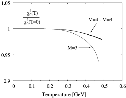
Figure 11: The temperature-dependent normalized minimum $\chi_{0}^{4}(T)/\chi_{0}^{4}(T=0)$ of the potential for different truncation orders $M$. ($\Lambda=2$ GeV, $h^{1/4}=0.69$ GeV, $\chi_{0}(\Lambda)=0.6$ GeV).

We therefore believe that we can trust the expansion of the dilaton potential up to a finite order $M$ when we are interested in temperatures below $200$ MeV. In a forthcoming publication [24] we are going to investigate the finite-temperature behavior of a scaled linear sigma model and study the influence of mesons on this result.

5 Conclusions and Outlook

We have investigated the thermal behavior of the gluon condensate within a self-consistent proper-time regularized Renormalization Group approach. An effective realization of the QCD trace anomaly by a scalar dilaton field is used, which yields a logarithmic potential parameterized by two constants. Due to the breakdown of the effective model for vanishing dilaton field, a perturbative analysis is not possible. Therefore, the order of the phase transition cannot be determine perturbatively. Using non-perturbative RG flow equations these difficulties can be circumvented and the calculation of the effective potential at the origin becomes possible.

We have considered two procedures to explore a possible phase transition in the effective dilaton model. First the full logarithmic potential is considered. The analysis is then compared to a truncated potential calculation where truncation errors are observed and discussed. The full potential analysis yields the potential for all dilaton fields and not only around the minimum. In contrast, the truncated potential calculation applies only in the vicinity of the global minimum.

At vanishing temperature, the model has been fixed to the glueball mass and bag constant. Our finite temperature predictions for the full potential are in good agreement with the results of Ref. [18] while the truncated potential calculation suffers from slow convergence and artificial truncation effects. Yet, the finite temperature results of the truncated potential calculation correspond qualitatively to those of the full potential analysis. One advantage of the truncated version is that a diagrammatical interpretation of the beta functions in terms of $n$-point vertices becomes possible, elucidating the underlying physics more clearly. The gluon condensate and the glueball mass remain unaltered up to temperatures of about 200 MeV where our prediction reaches its limit of validity due to the omission of temperature-dependent initial boundary conditions in the flow equations.

In contrast to [3] we do not observe any phase transition within the considered temperature range which makes the use of the expectation value of the dilaton field as an order parameter for the gluon deconfinement questionable. On the other hand this result is not astonishing, since the trace anomaly is not expected to vanish at high temperature [27].

We have neglected the influence of mesonic degrees of freedom which should anyhow play a minor role on the gluonic phase transition [18, 25, 26]. The consideration of these degrees of freedom in this RG framework is deferred to a forthcoming publication [24].

References

- [1] J. Schechter, Phys. Rev. D21 (1980) 3393;
- [2] H. Gromm, P. Jain, R. Johnson and J. Schechter, Phys. Rev. D33 (1986) 3476 and 801.
- [3] B.A. Campbell, J. Ellis and K.A. Olive, Phys. Lett. 235B (1990) 325; Nucl. Phys. B345 (1990) 57.
- [4] F. Karsch, hep-lat/0109017; To appear in the proceedings of QCD@Work: International Conference on QCD: Theory and Experiment, Martina Franca, Italy, 16-20 Jun 2001.
- [5] R. Floreanini and R. Percacci, Phys. Lett. B356 (1995) 205.
- [6] S.-B. Liao, Phys. Rev. D53 (1996) 2020.
- [7] C. Bagnuls and C. Bervillier, Phys. Rep. 348 (2001) 91.
- [8] O. Bohr, B.-J. Schaefer and J. Wambach, Int. J. Mod. Phys. A16 (2001) 3823 and references therein.
- [9] L. Dolan and R. Jackiw, Phys. Rev. D51 (1974) 3357.
- [10] C. Wetterich, Phys. Lett. B301 (1993) 90.
- [11] M. Mazza and D. Zappalà, hep-th/0106230.
- [12] A. Bonanno and D. Zappalà, Phys. Lett. B504 (2001) 181; D. Litim and J. Pawlowski, hep-th/0111191
- [13] G. Papp, B.-J. Schaefer, H.-J. Pirner and J. Wambach, Phys. Rev. D61 (2000) 096002.
- [14] B.-J. Schaefer and H.-J. Pirner, Nucl. Phys. A660 (1999) 439.
- [15] N. Tetradis and C. Wetterich, Int. J. Mod. Phys. A9 (1994) 4029.
- [16] K.M. Bitar et al., Nucl. Phys. B20 (Proc. Suppl.) (1991) 390.
- [17] Particle Data Group, Phys. Rev. D54 (1996) 1.
- [18] J. Sollfrank and U. Heinz, Z. Phys. C65 (1995) 111, nucl-th/940614.
- [19] J. Adams, J. Berges, S. Bornholdt, F. Freire, N. Tetradis and C. Wetterich, Mod. Phys. Lett. A10 (1995) 2367.
- [20] W. H. Press et al. Numerical Recipes, 2nd edition, (Cambridge University Press), 1992.
- [21] T.R. Morris, Prog. Theor. Phys. Suppl. 131 (1998) 395.
- [22] K.-I. Aoki et al., Prog. Theor. Phys. 95 (1996) 409 and Prog. Theor. Phys. 99 (1998) 451.
- [23] J. Alexandre, V. Branchina and J. Polonyi, Phys. Rev. D58 (1998) 016002; S.-B. Liao, C.-Y. Lin and M. Strickland, hep-th/0010100.
- [24] B.-J. Schaefer and J. Wambach, in preparation.
- [25] N.O. Agasian, D. Ebert and E.-M. Ilgenfritz, Nucl. Phys. A637 (1998) 135.
- [26] G.W. Carter, O. Scavenius, I.N. Mishustin and P.J. Ellis, Phys. Rev. C61 (2000) 045206.
- [27] H. Leutwyler, Deconfinement and Chiral Symmetry, in ’QCD 20 years later’, Vol. 2, P.M. Zervas and H.A. Kastrup (Eds.), World Scientific, Singapore (1993) 693.