Global Black Branes (Extended Global Defects Surrounded by Horizons), Brane Worlds and the Cosmological Constant

We study global defects coupled to higher-dimensional gravity with a negative cosmological constant. This paper is mainly devoted to studying global black brane solutions which are extended global defects surrounded by horizons. We find series solutions in a few separated regions and confirm numerically that they can be mutually connected. When the world volume of the brane is Ricci-flat, the brane is surrounded by a degenerated horizon, while it is surrounded by two horizons when the world volume has a positive constant curvature. Each solution corresponds to an extremal and a non-extremal state, respectively. Their causal structures resemble those of the Reissner-Nordström black holes in anti-de Sitter spacetime. However, the non-extremal black brane is not a static object, but an inflating brane. In addition, we briefly discuss a brane world model in the context of the global black branes. We comment on a few thermodynamic properties of the global black branes, and discuss a decrease of the cosmological constant on the brane world through the thermodynamic instability of the non-extremal global black brane.

I Introduction

Global defects are topologically stable scalar field configurations with nontrivial homotopy for some internal symmetry manifolds [1]. Usually, this kind of topological defect arises in a theory with $d$ scalar fields and a potential which has a vacuum manifold with the topology of a $(d-1)$-sphere. The simplest examples are domain walls [23, 24, 25] when the vacuum manifold has a discrete symmetry, global strings [2, 3] when $d=2$, and global monopoles [4] when $d=3$, in four spacetime dimensions. While the global monopole has a well-defined static metric, the domain wall and the global string do not. The domain wall spacetime is non-static and the metric in the plane of the domain wall is that of a $(2+1)$-dimensional de Sitter space. The spacetime of the global string has a curvature singularity at a finite distance from the string core [2]. Its metric was found by Cohen and Kaplan [3]. However, Gregory showed that time dependence could remove the singular nature of the global string spacetime [5]. While these analyses were purely within the context of Einstein gravity in four dimensions (in the absence of a cosmological constant), the global string spacetime is always regular in the presence of a negative cosmological constant [11], no matter how small cosmological constant may be. Because the negative cosmological constant could do a role to avoid the singularity rounding off the spacetime before it terminates at the singularity.

Global defects were first considered in four spacetime dimensions, but recently they have been studied in higher dimensions in the context of the brane world scenarios, such as the large extra dimension scenario (ADD) [7] and the Randall-Sundrum (RS) scenario [8, 9]. According to the brane world picture the three space dimensional world that we appear to be living in is a brane that is embedded in a higher-dimensional world. The brane world scenarios are really attractive in that the Newtonian gravity is recovered on the brane despite the gravity is fundamentally higher-dimensional one, even with large (infinite) extra dimensions. This approach provides a plausible explanation of the hierarchy between the gravitational and the electroweak mass scales, opening the possibility for construction of new classes of models for the unified theory. These theories also open new approaches to the cosmological constant problem, because if our four-dimensional world is embedded in a higher-dimensional spacetime, the effect of non-zero vacuum energy could affect only the curvature in the extra dimensions allowing for a flat four-dimensional world as first proposed in Ref. [39, 40, 41, 42, 43, 44].

There have been various attempts to realize the brane world scenario in the context of higher-dimensional gravitating global defects in Refs. [10, 11, 12, 13, 14, 15, 16, 17]. Cohen and Kaplan [10] have considered a brane world, which may be viewed as a global string in two extra dimensions. Its spacetime exhibits a curvature singularity at a finite distance from the string core, similar to the case in four dimensions. They argued that, imposing a unitary boundary condition, the location of the singularity may play a role of the boundary of the extra dimensions, which form a finite but non-compact space of exponentially large proper size. The phenomenology resembles the ADD scenario, rather than that of the RS scenario. Gregory [11] has shown that a non-singular global string-like solution with the required properties for the RS-type scenario exists in the presence of a negative bulk cosmological constant. Olasagasti and Vilenkin [12] explored a more general case of a brane carrying a global charge in a higher-dimensional spacetime with a nonzero cosmological constant. In particular, with a negative cosmological constant there exist solutions of which the geometry of extra dimensions asymptotes to a cylinder with cross section being a $(d-1)$-sphere of a fixed radius (cigar-like geometry). The cigar-like solutions with an exponentially decaying warp factor is of interest, since they have features needed for the RS-type scenario.

On the other hand, in Ref. [16] the authors investigated the spacetime of higher-dimensional global defects in the presence of a negative cosmological constant adopting Schwarzschild-type metric ansätz. They found extremal black hole-like $p$ space dimensional defects (global black $p$-branes), which are Ricci-flat branes surrounded by a degenerated horizon. They showed that the near horizon geometry of the extremal global black branes coincides with the cigar-like geometry with an exponentially damping warp factor discovered in Refs. [11, 12]. The interior region inside the horizon of the global black $p$-brane possesses all of features needed for a brane world with the Newtonian gravity. In the picture of Ref. [16] the size of the horizon can be interpreted as the compactification size of $d$ extra dimensions, even though the interior region inside the horizon infinitely extends and asymptotes to $AdS_{p+2}\times S^{d-1}$. Therefore, the large mass hierarchy is translated into the large size of the horizon, which could be supported by the large magnitude of charge carried by the black branes. In this picture, the Hawking radiation could be a possible mechanism for the resolution of various problems associated with brane world scenarios, such as the observed flatness and the approximate Lorentz invariance of our world. The bending of the brane and the bulk curvature that violate the $SO(3,1)$ isometry on our brane [37, 38] would correspond to excitations upon the extremal state, and the excited states that are non-extremal black branes would evolve into an extremal state through the Hawking radiation process.

The nonzero vacuum energy density (equivalently, the cosmological constant) on the brane could also be an excitation upon the extremal state, which would be diluted via the Hawking process if the excited state correspond to a non-extremal black brane. However, even though the state excited by the vacuum energy density is a non-extremal state, it will be somehow different from static non-extremal black branes treated usually in the literatures before in the context of supergravity or string theories [22], because with nonzero vacuum energy density the branes will inflate and the corresponding spacetime will not be static. Therefore, their thermodynamic properties will also be different from those of the static ones. In this respect, we may need to find the corresponding black brane solutions and to examine their thermodynamic properties, to see whether a certain thermodynamic process can be a dynamical mechanism thinning out the vacuum energy density on the brane.

This paper will be mainly devoted to finding global black brane solutions which are extended global defects surrounded by horizons and studying their spacetime structures. However, we will also focus on a few aspect of a brane world based on the global black branes and the cosmological constant problem.

This paper is organized as follows. In Sec. II, we derive the equations of motion corresponding to the Schwarzschild-type metric ansätz in a scalar theory with global internal symmetry coupled to higher-dimensional gravity with a negative cosmological constant. In Sec. III, we explore black hole-like $p$ space dimensional defect (black $p$-brane) solutions, which shall be referred in what follows as “global black $p$-brane” or “global black brane”. We find series solutions in a few separated regions and confirm numerically that they can be mutually connected. When the world volume of the branes is Ricci-flat, the branes are surrounded by a degenerated horizon, while when the world volume is not Ricci-flat but of a positive constant curvature, they are surrounded by two horizons. They correspond to extremal black branes and non-extremal ones, respectively. In Sec. IV, we discuss the spacetime structures of the global black branes. Their causal structures resemble those of the Reissner-Nordström black holes in anti-de Sitter spacetime, if we consider the transverse slice to the brane. The near horizon geometries are an infinitely long anti-de Sitter throat with the topology of $AdS_{p+2}\times S^{d-1}$ for the extremal black branes, and the spacetime of an inflating $p$ space dimensional domain wall times $(d-1)$-dimensional sphere for non-extremal ones. In Sec. V, we discuss a few issues associated to the brane world scenarios. We briefly comment a few thermodynamic properties of the global black branes, and discuss a decrease of the cosmological constant on the brane world through the thermodynamic instability of the non-extremal global black brane. In the last section, we end with some conclusions.

II The Equations of Motion

In this section we derive field equations appropriate to isolated gravitating global defects in higher-dimensional spacetime with a negative cosmological constant. Higher-dimensional gravitating global defects are described as topologically stable scalar field configurations of a field theory with a spontaneously broken continuous global symmetry coupled to $D$-dimensional gravity. We consider a scalar theory with global $O(d)$ symmetry coupled to gravity, of which potential has minimum on the $(d-1)$-sphere of radius $v^{2}$:

$$S = S_{{\rm gravity}}+S_{{\rm scalar}}$$ (1)

$$S_{{\rm gravity}} = \frac{M^{D-2}_{*}}{16\pi}\int dx^{D}\sqrt{g_{D}}~{}(R-2\Lambda)$$ (2)

$$S_{{\rm scalar}} = \int dx^{D}\sqrt{g_{D}}\left[-\frac{1}{2}\nabla_{M}\phi^{a}\nabla^{M}\phi^{a}-\frac{\lambda}{4}(\phi^{b}\phi^{b}-v^{2})^{2}\right],$$ (3)

where $M_{*}$ is the fundamental scale of the higher-dimensional gravity theory. We use a mostly plus signature. Note that $\phi^{a}$ and $v$ have a mass dimension of $(p+d-1)/2$ and the negative bulk cosmological constant ($\Lambda<0$) has a mass dimension of 2. This theory admits $p$ space dimensional topological solitons, where $p+1=D-d$. We shall refer them as ‘global $p$-brane’ in what follows. $M,N,...$ denote $D$-dimensional spacetime indices and $a,b,...$ do $d$-dimensional internal space indices and run on $1,...,d$. We shall use the notation $\{x^{\mu}\}$ with $\mu=0,...,p$ for the coordinates on the $p$-brane world volume. $\{y^{a}\}$ denote the transverse coordinates to the $p$-brane and are related to the spherical coordinates of the transverse space by the usual relations: $y^{a}=\{r\cos\theta_{1},\cdots\cdots,r\sin\theta_{1}\cdots\cos\theta_{d-1},r\sin\theta_{1}\cdots\sin\theta_{d-1}\}$ with $r^{2}=y^{a}y^{a}$. The corresponding Einstein equations and scalar field equation are

$$R_{M}{}^{N}=\frac{8\pi}{M_{*}^{D-2}}{\cal T}_{M}{}^{N}+\delta_{M}{}^{N}\frac{2}{D-2}\Lambda,$$ (4)

$$\nabla_{M}\nabla^{M}\phi^{a}-\lambda(\phi^{b}\phi^{b}-v^{2})\phi^{a}=0,$$ (5)

where

$${\cal T}_{M}{}^{N}\equiv\nabla_{M}\phi^{a}\nabla^{N}\phi^{a}+\delta_{M}{}^{N}\frac{\lambda}{2(D-2)}(\phi^{b}\phi^{b}-v^{2})^{2}.$$ (6)

The global defects are defined by a topologically nontrivial mapping of the vacuum manifold $O(d)/O(d-1)$ to the boundary of transverse dimensions $S^{d-1}$. We take ansätz for the scalar field configuration as:

$$\phi^{a}=vX~{}y^{a},$$ (7)

where the function $X$ could be a function of both $t$ and $r$ in general. The defect solution should have $X(r=0)=0$ at the center of the defect and approach the radial ‘hedgehog’ configuration outside the core.

In this paper, we consider a particular case that the energy-momentum tensor of the defects is time independent. As a result, no gravitational and particle radiation exists. The spacetime section transverse to the defects is static, and the whole spacetime including longitudinal directions is allowed to be static or stationary as we will see later. The spacetime of the extended global defects have the topology of $R^{p+2}\times S^{d-1}$. For black branes, the spacetime transverse to the brane will be a generalization of the $4$-dimensional spherically symmetric solutions, e.g. the Schwarzschild or the Reissner-Nordström black hole solutions. To obtain these solutions of the Einstein equations we will assume that outside any horizon there is a Killing vector which is timelike and that surfaces of constant $t$ are formed from concentric $(d-1)$-spheres times $p$-dimensional space. We can then quite generally adopt following Schwarzschild-type metric ansätz:

$$ds^{2}=e^{2A(r)}B(r)\hat{g}_{\mu\nu}(x)dx^{\mu}dx^{\nu}+\frac{dr^{2}}{B(r)}+r^{2}d\Omega_{d-1}^{2},$$ (8)

where $\hat{g}_{\mu\nu}(x)$ is a metric on $(p+1)$-dimensional brane world volume which is not necessarily static, $d\Omega_{d-1}^{2}$ is the line element on the unit $(d-1)$-sphere, and $A(r)$ and $B(r)$ are functions of $r$ only. With this metric ansätz, the defect solutions with unit winding number correspond to the field configurations

$$\phi^{a}=vf(r)\frac{y^{a}}{r}.$$ (9)

The defect solutions have $f(r)=0$ at the center and approach $f(r)\simeq 1$ outside core. The energy-momentum tensor for the field configuration (9) is then given by

$$\hat{\cal T}_{t}{}^{t} = \hat{\cal T}_{x_{i}}{}^{x_{i}}=\frac{(1-f^{2})^{2}}{2(p+d-1)},$$ (10)

$$\hat{\cal T}_{r}{}^{r} = Bf^{\prime 2}+\frac{(1-f^{2})^{2}}{2(p+d-1)},$$ (11)

$$\hat{\cal T}_{\theta_{a}}^{\theta_{a}} = \frac{f^{2}}{r^{2}}+\frac{(1-f^{2})^{2}}{2(p+d-1)},$$ (12)

where $\hat{\cal T}^{M}_{\;N}={\cal T}^{M}_{\;N}/\lambda v^{4}$.

Since the metric (8) is a special case of the more general class of metric,

$$ds^{2}=F(y^{a})^{2}d\hat{s}^{2}+d\tilde{s}_{d}^{2},$$ (13)

where $d\tilde{s}_{d}^{2}$ is the metric of the slice in the transverse directions and $d\hat{s}^{2}$ is the world volume metric, the Ricci tensor splits in the following way:

$$R_{\mu\nu} = \hat{R}_{\mu\nu}-\hat{g}_{\mu\nu}[F\tilde{\nabla}^{2}F+p(\tilde{\nabla}F)^{2}]$$ (14)

$$R_{ab} = \tilde{R}_{ab}-(p+1)\frac{\tilde{\nabla}_{a}\tilde{\nabla}_{b}F}{F}.$$ (15)

Since ${\cal T}_{\mu\nu}\propto\hat{g}_{\mu\nu}$, through Einstein’s equations we have that $R_{\mu\nu}\propto\hat{g}_{\mu\nu}$ and finally, from Eq. (14) above, that $\hat{R}_{\mu\nu}\propto\hat{g}_{\mu\nu}$. That is, $\hat{R}$, the curvature associated with the metric $\hat{g}_{\mu\nu}$, must be constant[12]. Therefore, without losing generality we can assume that the spatial part of the metric intrinsic to the brane is homogeneous and isotropic, and the directions parallel to the brane are boost invariant in the strong sense. Einstein’s field equations then reduce to

$$\frac{1}{p+1}\frac{\hat{R}}{e^{2A}B}-(p+1)BA^{\prime 2}-\frac{2p+3}{2}B^{\prime}A^{\prime}-\frac{p}{4}\frac{B^{\prime 2}}{B}-BA^{\prime\prime}-\frac{1}{2}B^{\prime\prime}$$ (16)

$$-\frac{d-1}{r}\left(BA^{\prime}+\frac{1}{2}B^{\prime}\right)=8\pi G_{D}\hat{{\cal T}}_{t}{}^{t}+\frac{2}{p+d-1}\Lambda,$$ (17)

$$-(p+1)\left(BA^{\prime 2}+\frac{3}{2}B^{\prime}A^{\prime}+BA^{\prime\prime}+\frac{1}{2}B^{\prime\prime}\right)-\frac{d-1}{2}\frac{B^{\prime}}{r}=8\pi G_{D}\hat{{\cal T}}_{r}{}^{r}+\frac{2}{p+d-1}\Lambda,$$ (18)

$$-(p+1)\frac{BA^{\prime}}{r}-\frac{p+2}{2}\frac{B^{\prime}}{r}-(d-2)\frac{B-1}{r^{2}}=8\pi G_{D}\hat{{\cal T}}_{\theta_{a}}{}^{\theta_{a}}+\frac{2}{p+d-1}\Lambda,$$ (19)

supplemented by the equation for the metric on the $p$-brane,

$$\hat{R}_{\mu\nu}=\frac{\hat{R}}{p+1}\hat{g}_{\mu\nu}.$$ (20)

It can be easily shown that only two of the three equations (17)-(19) are independent. The scalar field equation is written down as

$$f^{\prime\prime}+\left[\frac{d-1}{r}+\left(1+\frac{p}{2}\right)\frac{B^{\prime}}{B}+(1+p)A^{\prime}\right]f^{\prime}-\frac{1}{B}\left[\frac{(d-1)}{r^{2}}+(f^{2}-1)\right]f=0.$$ (21)

Here we have defined a dimensionless Newtonian constant $G_{D}\equiv v^{2}/M_{\ast}^{D-2}$ and we have rescaled the coordinates and redefined the cosmological constant as

$$\sqrt{\lambda}vx_{M}\rightarrow x_{M},~{}~{}{\rm and}~{}~{}~{}\Lambda/\lambda v^{2}\rightarrow\Lambda.$$ (22)

III Solutions

We may be able to find several classes of solutions to the set of field equations (17)-(21). However, we will restrict our discussion to only black hole-like solutions in this paper. First, we find extremal black brane solutions which are flat branes surrounded by a degenerated horizon. Next we shall discuss about non-extremal black brane solutions which are bent branes surrounded by two horizons.

For the simplest case (of $p=0$ and $d=2$) which corresponds to a vortex in $(2+1)$-dimensional spacetimes, the global vortex solutions were thoroughly analyzed for the global $U(1)$ scalar theory in Ref.[19] and for the $O(3)$ nonlinear $\sigma$ model in Ref.[20] in the presence of a negative cosmological constant. For the global $U(1)$ theory, there are three types of solutions depending on the relative scales of parameters of the theory: the cosmological constant, the Planck scale and the symmetry breaking scale. They are regular vortex, extremal and non-extremal Reissner-Nordström-type black holes carrying topological charges. Their spacetimes are perfectly regular and do not involve any physical curvature singularity. When the magnitude of a negative cosmological constant is larger than a critical value at a given symmetry breaking scale, the spacetime formed by a isolated vortex is regular hyperbola with a deficit angle. However, it becomes a charged black hole when the magnitude of the cosmological constant is less than the critical value. For the $O(3)$ nonlinear $\sigma$ model, the usual regular topological lump solution cannot form a black hole even though the scale of symmetry breaking is increased. There exist non-topological solitons of half integral winding in the given model, and the corresponding spacetimes involve charged BTZ black holes.

When $p\geq 1$ and $d\geq 2$, the equations of motion, however, become much more nonlinear as can be seen from Eqs. (17)-(21). Due to this high nonlinearity of Eqs. (17)-(21), the spacetime around the global $p$-brane may develop a curvature singularity in an analogous fashion to the four-dimensional global string metric (with vanishing cosmological constant) [2, 3]. In other side, we may also expect that the bulk negative cosmological constant could do a role to avoid the singularity rounding off the spacetime before it terminates at the singularity [11]. As discussed in Ref. [12], the spacetime structure of global extended defects are depends on the number of extra dimensions $d$, the bulk cosmological constant $\Lambda$, and the $p$-brane world volume curvature $\hat{R}$. For a negative cosmological constant. When $\hat{R}=0$, every spacetime found in Ref. [12] are regular without any genuine singularity. When $\hat{R}\neq 0$, some of the spacetimes has singularity at a finite proper distance from the core.

We will see that, for black hole-like solutions, cases $\hat{R}=0$ correspond to extremal black $p$-branes, while cases $\hat{R}\neq 0$ to the non-extremal states. The black brane solutions are perfectly regular ones. Moreover, we will show that some of the independent solutions found in Ref. [12] actually describe different regions of the spacetime of a global black brane.

A Extreme black branes: flat branes surrounded by a degenerated horizon

Now we will analyze the equations derived in the previous section for the isolated global defect spacetime and find solutions of which world volume is Ricci-flat, i.e., $\hat{R}=0$. We will see that such branes correspond to extremal black branes, if it has a horizon. Since it seems almost impossible to find out exact analytic solutions of equations of motion Eqs. (17)-(21), we will just try to examine the behavior of the global $p$-brane spacetime at a few separated regions. Outside the core, the energy-momentum tensor is approximated into

$$\hat{\cal T}_{t}{}^{t}=\hat{\cal T}_{x_{i}}{}^{x_{i}}\simeq\hat{\cal T}_{r}{}^{r}\simeq 0~{}~{}~{}{\rm and}~{}~{}~{}\hat{\cal T}_{\theta_{a}}^{\theta_{a}}\simeq\frac{1}{r^{2}},$$ (23)

with $f(r)\simeq 1$. Therefore, outside the core the behavior of the solutions is determined solely by the relative magnitude of the scalar field energy density ($8\pi G_{D}/r^{2}$) to the cosmological constant ($|\Lambda|$) through the equation (19).

Near the origin where the field energy density dominates over the cosmological constant, the series solution up to the leading term is as follows:

$$f(r) \approx f_{0}~{}r,$$ (24)

$$A(r) \approx A_{0}+A_{2}~{}r^{2},$$ (25)

$$B(r) \approx 1+B_{2}~{}r^{2},$$ (26)

where $f_{0}$ is a shooting parameter to be determined by the proper behavior of the fields at the asymptotic region, and $A_{0}$ can be consistently fixed as $A_{0}=0$ so that the spacetime is locally Minkowski at the origin. The coefficients $A_{2}$ and $B_{2}$ are given as follows

$$A_{2} \equiv \left[\frac{4\pi G_{D}}{d-1}\left(f_{0}^{2}-\frac{p}{2d(p+d-1)}\right)+\frac{p|\Lambda|}{d(d-1)(p+d-1)}\right],$$ (27)

$$B_{2} \equiv -\left[\frac{8\pi G_{D}}{d-1}\left(f_{0}^{2}-\frac{p-d+1}{2d(p+d-1)}\right)+\frac{2(p-d+1)|\Lambda|}{d(d-1)(p+d-1)}\right].$$ (29)

While the metric function $A(r)$ increases, $B(r)$ decreases near the origin for generic values of $f_{0}$. With this solution the metric Eq. (8) near the core takes the form of

$$ds^{2}\approx\left[1-\frac{4\pi G_{D}-2|\Lambda|}{d(p+d-1)}r^{2}\right]\bar{g}_{\mu\nu}(x)dx^{\mu}dx^{\nu}+\frac{dr^{2}}{1+B_{2}r^{2}}+r^{2}d\Omega_{d-1}^{2},$$ (30)

where $\bar{g}_{\mu\nu}(x)$ is a general Ricci-flat metric on the brane, which satisfies $(p+1)$-dimensional vacuum Einstein equations $\bar{R}_{\mu\nu}(\bar{g})=0$. This shows that the metric component $g_{00}$ of the spacetime decrease in the transverse directions near the origin when $2\pi G_{D}>|\Lambda|$, regardless value of $f_{0}$. This fact implies a possibility that the $(00)$-th component of the metric could vanish at a finite coordinate distance and of the formation of black hole-like defects, when $2\pi G_{D}>|\Lambda|$.

In the far region from the core where the cosmological constant dominates over the scalar fields energy density, the metric functions behave up to the leading terms for sufficiently large $r$ as follows:

$$f(r) \approx 1,$$ (31)

$$A(r) \approx A_{\infty}+\frac{(p+d)(p+d-1)(8\pi G_{D}-d+2)}{8(p+1)|\Lambda|}~{}\frac{1}{r^{2}},$$ (32)

$$B(r) \approx \frac{2|\Lambda|}{(p+d)(p+d-1)}~{}r^{2},$$ (33)

where $A_{\infty}$ is a constant to be determined by matching with series solutions in other regions. The metric (8) then is

$$ds^{2}\approx B_{\infty}r^{2}~{}\bar{g}_{\mu\nu}(x)dx^{\mu}dx^{\nu}+\frac{dr^{2}}{B_{\infty}r^{2}}+r^{2}d\Omega_{d-1}^{2},$$ (34)

where $\exp(2A_{\infty})$ has been absorbed into the longitudinal coordinates $x_{\mu}$ and $B_{\infty}\equiv 2|\Lambda|/(p+d)(p+d-1)$. This asymptotes to $D$-dimensional anti-de Sitter spacetime ($AdS_{D}$) with $\bar{g}_{\mu\nu}(x)=\eta_{\mu\nu}$, as we will see in next section.

We now turn to the intermediate region, at which the scalar energy density and the cosmological constant is comparable, between the core and the asymptotic regions described by metrics (30) and (34), respectively. From the behavior of $g_{00}$, we may expect that a horizon is located in the intermediate region. Since what we are looking for is the existence of a black hole horizon, it will be convenient to write the metric component $g_{00}$ in terms of $B(r)$ and $f(r)$ by eliminating $A(r)$ with use of Eq. (19) as

$$e^{2A}B = C~{}r^{-\frac{2(d-2)}{(p+1)}}B^{-\frac{1}{(p+1)}}$$ (36)

$$\times\exp\left[-\frac{2}{p+1}\int^{r}\left(\frac{8\pi G_{D}f^{2}-d+2}{r}-\frac{2|\Lambda|-4\pi G_{D}(1-f^{2})^{2}}{p+d-1}~{}r\right)\frac{dr}{B}\right],$$

where $C$ is an integral constant and it can be set to be $1$ with the boundary condition $A=0$ at $r=0$. To examine the existence and the property of the horizon, we begin assuming that there exists a horizon at a finite coordinate distance $r_{H}$ from the core or the asymptotic region, so that the timelike Killing vector $\partial_{t}$ becomes null there, that is, $\exp[2A(r_{H})]B(r_{H})=0$. Further we assume that $B(r)$ becomes zero and is analytic at the horizon. However, we don’t put further restriction on $A(r)$ because it could be singular at $r=r_{H}$, as can easily be observed from Eq. (19). We also assume that the scalar field $f(r)$ increases monotonically to unit value and behaves regularly at the horizon. Then the position of the horizon $r_{H}$ and the value of $f_{H}(\equiv f(r_{H}))$ are determined in a closed form from the field equations.

Multiplying $e^{2A}B$ on Eq. (17), eliminating $A^{\prime}$ and $A^{\prime\prime}$ with Eq. (19), and taking the limit $r\to r_{H}$, we obtain

$$e^{2A(r_{H})}\left[B_{1}+\Delta\right]\left[B_{1}+2\Delta\right]=0,$$ (37)

where $B_{1}\equiv B^{\prime}(r_{H})$ and

$$\Delta\equiv\frac{8\pi G_{D}f_{H}^{2}-d+2}{r_{H}}-\frac{2|\Lambda|-4\pi G_{D}(1-f_{H}^{2})^{2}}{p+d-1}r_{H}.$$ (38)

On the other hand, eliminating $A^{\prime}$, $A^{\prime\prime}$ from Eqs. (18) and (19), and taking the limit $r\to r_{H}$, we get

$$\left[(p+2)B_{1}+2\Delta\right]\left[B_{1}+2\Delta\right]=0.$$ (39)

There are two possibilities for $B_{1}$ satisfying simultaneously the two relations Eqs. (37) and (39): $B_{1}=-2\Delta\neq 0$ or $B_{1}=0=\Delta$. However, the former possibility should be excluded because with such condition the metric component $g_{00}(r_{H})$ does not vanish, but approaches to a non-zero value at $r=r_{H}$, leading to a contradiction with our starting assumption. This can easily be checked by inserting following series expansions into Eq. (36)

$$B(r) \approx B_{1}(r-r_{H})+B_{2}(r-r_{H})^{2}+B_{3}(r-r_{H})^{3}+\cdot\cdot\cdot,$$ (40)

$$f(r) \approx f_{H}+f_{1}(r-r_{H})+f_{2}(r-r_{H})^{2}+\cdot\cdot\cdot.$$ (41)

The latter possibility only is acceptable and satisfies the condition for the surface at $r=r_{H}$ to be a horizon. Inserting above series expansions into Eq. (36) and using $B_{1}=0=\Delta$ give up to the leading term

$$e^{2A}B\sim(r-r_{H})^{\frac{1}{p+1}\left[-1+\frac{4}{B_{H}}\frac{2|\Lambda|-4\pi G_{D}(1-f_{H}^{2})^{2}}{p+d-1}\right]},$$ (42)

where we have replaced $B_{2}$ with $B_{H}$, i.e. $B_{2}\equiv B_{H}$. Therefore, if $B_{H}<4[2|\Lambda|-4\pi G_{D}(1-f_{H}^{2})^{2}]/(p+d-1)$, $e^{2A}B$ touches zero at $r=r_{H}$. We will see later that this condition is always satisfied. Since $\Delta=0$, from Eq. (38) we find the position of the horizon in a closed form

$$r_{H}^{2}=\frac{(p+d-1)(8\pi G_{D}f_{H}^{2}-d+2)}{2|\Lambda|-4\pi G_{D}(1-f_{H}^{2})^{2}}.$$ (43)

The fact $B^{\prime}(r_{H})=0$ indicates that the horizon is degenerated like that of an extremal black brane. This tells that the black $p$-brane solution with Ricci-flat world volume is extremal, as we have expected.

Inserting series expansions Eqs. (40) and (41) (with $B_{1}=0$) into Eq. (19) and using the condition $\Delta=0$, one finds that

$$A^{\prime}(r)\approx\frac{\alpha}{r-r_{H}}+O[(r-r_{H})^{0}],$$ (44)

where

$$\alpha\equiv\frac{1}{p+1}\left[p+2-2\frac{2|\Lambda|-4\pi G_{D}(1-f_{H}^{2})^{2}}{(p+d-1)B_{H}}-p\frac{16\pi G_{D}(1-f_{H}^{2})f_{H}r_{H}f_{1}}{(d-1)(p+d-1)B_{H}}\right],$$ (45)

Here, the coefficients $B_{H}$, $f_{H}$, and $f_{1}$ can be determined in terms of parameters given in the theory using the equations of motion. Thus $A(r)$ is at most logarithmically divergent at $r=r_{H}$:

$$A(r)\approx-\alpha\ln(r-r_{H})+O[(r-r_{H})^{0}],$$ (46)

and the $(00)$-component of the metric then becomes

$$g_{00}=e^{2A(r)}B(r)\approx B_{H}(r-r_{H})^{2(1-\alpha)}.$$ (47)

With series expressions of $B(r)$, $f(r)$ and $A(r)$ at the horizon, from Eqs. (17) and (19) we obtain

$$B_{H}(1-\alpha)^{2}=\frac{2|\Lambda|-4\pi G_{D}(1-f_{H}^{2})^{2}}{(p+1)(p+d-1)},$$ (48)

and then simultaneously solving this and Eq. (45) for $B_{H}$ and $\alpha$, we get

$$1-\alpha = \frac{1}{2(2+\gamma)}\left[1\pm\sqrt{\frac{p+9+4\gamma}{p+1}}\right],$$ (49)

$$B_{H} = \frac{|\Lambda|-2\pi G_{D}(1-f_{H}^{2})^{2}}{p+d-1}\left[(p+5+2\gamma)\mp\sqrt{(p+1)(p+9+4\gamma)}~{}\right],$$ (51)

where

$$\gamma\equiv\frac{16\pi pG_{D}r_{H}(1-f_{H}^{2})f_{H}f_{1}}{(d-1)(2|\Lambda|-4\pi G_{D}(1-f_{H}^{2})^{2})}.$$ (52)

For lower sign, $(1-\alpha)$ is negative. This branch of solutions should be excluded because, in that case, the norm of $\partial_{t}$ ($=e^{2N}B$) will diverge at $r=r_{H}$, leading to a contradiction with our starting assumption that $g_{00}$ is zero at $r=r_{H}$. We will discuss more about this branch in next section. Whereas, with the upper sign $(1-\alpha)$ is positive saying that the surface of $r=r_{H}$ is a horizon. $B_{H}$ satisfy our starting assumption that $e^{2A}B\to 0$ as $r\to r_{H}$, as can be seen from Eq. (42). The coefficient $f_{1}$ can be completely determined in terms of $r_{H}$ and $f_{H}$ using Eqs. (21), (40), (41) and (44):

$$f_{1}=\frac{(d-1)f_{H}/r_{H}-(8\pi G_{D}f_{H}^{2}-d+2)}{r_{H}^{2}\left(p\displaystyle{\frac{8\pi G_{D}f_{H}}{(p+d-1)r_{H}}}-f_{H}^{2}\right)}.$$ (53)

On the other hand, considering limiting behaviors of the scalar field and the metric functions at the horizon, from the scalar field equation Eq. (21) we obtain another relation for $r_{H}$ and $f_{H}$

$$r_{H}^{2}=\frac{d-1}{1-f_{H}^{2}}.$$ (54)

Solving simultaneously the two equations (43) and (54), $r_{H}$ and $f_{H}$ can be expressed in terms of parameters in the theory, $\Lambda$ and $G_{D}$, as

$$r_{H}^{2} = \frac{(p+d-1)(8\pi G_{D}-d+2)}{4|\Lambda|}\left[1\pm\sqrt{1-\frac{32\pi G_{D}|\Lambda|(d-1)(2p+d-1)}{(8\pi G_{D}-d+2)^{2}(p+d-1)^{2}}}~{}\right],$$ (55)

$$f_{H}^{2} = \frac{p}{2p+d-1}+\frac{(p+d-1)}{8\pi G_{D}(2p+d-1)}\left[\frac{}{}\right.(d-2)$$ (57)

$$\left.\pm(8\pi G_{D}-d+2)\sqrt{1-\frac{32\pi G_{D}|\Lambda|(d-1)(2p+d-1)}{(8\pi G_{D}-d+2)^{2}(p+d-1)^{2}}}~{}\right].$$

The complete determination of the position of the horizon $r_{H}$ and the value of the scalar amplitude $f_{H}$ is an inevitable result since the leading term of Einstein equations Eqs. (17)-(19) and the scalar field equation (21) lead to two algebraic equations for $r_{H}$ and $f_{H}$. The coefficients $B_{3}$ and $f_{1}$ are expressed in terms of $r_{H}$ and $f_{H}$ by using the field equations, so $B_{3}$ and $f_{1}$ also are completely determined in terms of the parameters of the theory. Since the higher order coefficients of the series expansions (40) and (41) can be expressed in terms of lower order coefficients, every coefficients can be determined completely in closed forms. This implies that the flat brane solution with horizon is unique for given parameters of the theory.

The size of the horizon ($r_{H}$) and the value of scalar field at the horizon ($f_{H}$) have two different expression for parameters given in the theory, that is, we have two different types of black brane solutions. For the first type of solutions with lower sign, the horizon is formed inside the brane core and the bulk cosmological constant has to be super-Planckian for generic values of symmetry breaking scale of the theory. The condition that $f_{H}^{2}$ should be positive and real requires that the bulk cosmological constant have a value within a limited region above the Planck scale:

$$2\pi G_{D}-\frac{(d-2)(p+d-1)}{2}<|\Lambda|<\frac{(8\pi G_{D}-d+2)^{2}(p+d-1)^{2}}{32\pi G_{D}(d-1)(2p+d-1)}.$$ (58)

For this value of the bulk cosmological constant, the core size of a black brane will be larger than the size of the horizon. As an example, for $p=3,~{}d=2$ the value of the scalar field at the horizon is at most $\sqrt{3/7}$ showing that the core region extends outward beyond the horizon. Then, solutions of this sort may be viewed as small black branes lying within larger global branes. However, these solutions may develop a classical instability in a similar way to the case of the magnetically charged Yang-Mills solitonic black holes with sufficiently small horizon [21]. This instability may lead to the possibility that such a black brane could evaporate completely, leaving in its place a nonsingular global defect. The question of whether the black branes with small horizon lead to similar instabilities discussed in Ref. [21] itself will be an interesting one, but is beyond the scope of this paper.

On the other hand, for solutions with upper sign the mass scale of the bulk cosmological constant could be well below the Planck scale and the horizon can be formed far outside the brane core for generic values of the symmetry breaking scale and the bulk cosmological constant, as can easily be checked in Eq. (57). Solutions of this sort will be matched smoothly to a version of ‘thin-wall approximation’ found in Ref. [16]. In this paper, we will consider only the black brane solutions corresponding to the upper sign, because we are interested in only solutions with horizon larger than brane core with respect to the brane world scenario of Ref. [16].

The metric Eq. (8) then has the form near $r=r_{H}$

$$ds^{2}\approx B_{H}[\sigma(r-r_{H})]^{2(1-\alpha)}\bar{g}_{\mu\nu}(x)dx^{\mu}dx^{\nu}+\frac{dr^{2}}{B_{H}(r-r_{H})^{2}}+r_{H}^{2}d\Omega_{d-1}^{2},$$ (59)

where $\sigma$ is $+1$ for the exterior region ($r>r_{H}$) and $-1$ for the interior region ($r<r_{H}$). Note that, so far, we have implicitly assumed that we examine the near horizon region from the outside toward the horizon at $r_{H}$ and hence obtained only exterior metric ($\sigma=1$). Had we done from the outside region, we would then obtain the interior metric ($\sigma=-1$).

Up to now, finding an exact analytic solution to the field equations Eqs. (17)-(21) being impossible, we have examined behavior of the solution of the global $p$-brane at a few separated regions. The spacetime of the global black $p$-brane will be described via metrics Eqs. (30), (34) and (59) provided that they are connected mutually. For metric functions, $A(r)$ increases near the origin, diverges at $r_{H}$ and decreases and rapidly approaches to a constant value at the asymptotic region, as can be seen from Eqs. (25), (32) and (46). $B(r)$ decreases near the origin, vanishes at $r_{H}$ and increases quadratically at the asymptotic region, as indicated in Eqs. (26), (33) and (40). The scalar field $f(r)$ starts to grow linearly from zero at the origin, reaches to a fixed value $f_{H}$ of Eq. (57) and then approaches to its vacuum value at the asymptotic region. From the behaviors of the metric functions and scalar field, we can easily guess that the fragments of solution can be connected mutually if they behaves monotonically at each side of the horizon.

FIG. 1.: A flat 3-brane solution surrounded by a degenerated horizon with two transverse directions $(d=2)$ when $G_{D}=0.15$ and $|\Lambda|=0.420872997$. With the thick solid line we report the behavior of the metric function $B(r)$ and with the dashed line the behavior of the scalar field $f(r)$, whereas with the thin solid line the behavior of $A^{\prime}(r)$.

While we have not resolved yet whether the solutions obtained in separated regions can be connected mutually or not, numerical calculations indicate that the metric functions and the scalar field behave monotonically at each side of the horizon, and the solutions obtained in separated regions are connected smoothly showing the existence of the black $p$-brane solution. Such an example of the black brane solution is shown in FIG.1. The obtained solution is for an extremal black 3-brane with two transverse spatial direction $(d=2)$, that is, a global black string-like defect. The scalar field $f(r)$ (the dashed line) behaves monotonically for every $r$ and connects $f(0)=0$ and $f(\infty)=1$ smoothly across the horizon at $r=r_{H}$. The metric function $B(r)$ (the thick solid line) decreases monotonically inside the horizon and vanishes at the horizon $r_{H}$, and then increases monotonically. On the other hand, the derivative of the metric function $A(r)$ (the thin solid line) shows a singular behavior at the horizon as shown in Eq. (44).

Before ending this section, we briefly discuss the scales of parameters of the theory: the symmetry breaking scale $v$, the Planck scale $M_{*}$ and the cosmological constants $\Lambda$. The right-hand side of Eq. (43) ought to be positive. This condition yields $v^{2}>((d-2)/8\pi)~{}M_{*}^{D-2}$. While the condition does not give any new information for $d=2$, for $d>2$, the condition sets the symmetry breaking scale $v$ to be of the order of the fundamental scale $M_{*}$. On the other hand, in order to trust the theory, $v^{2/D-2}$ ought to be smaller than the fundamental scale: $v^{2/D-2}<M_{*}$. Hence, we assume that $(d-2)/8\pi<v^{2}/M_{*}^{D-2}<1$. We also assume that $v^{2/D-2}<M_{*}$ even for $d=2$, but this seems valid for naturalness reasons. The horizon size $r_{H}$ is then determined by the bulk cosmological constant $\Lambda$, viz, $r_{H}^{-2}\sim|\Lambda|$. There is no restriction on the scale of the cosmological constant. It seems to be natural that the cosmological constant is of the order of the fundamental scale in the absence of a mechanism to protect a small cosmological constant from radiative corrections. However, given our ignorance concerning the bulk cosmological constant problem, there is a priori no reason to expect that $\Lambda$ is of the same order as the fundamental scale $M_{*}^{2}$. Thus, we will treat the cosmological constant $\Lambda$ simply as an input parameter.

B Non-extremal black branes: bent branes surrounded by two horizons

In the previous subsection we found extremal black brane-like solutions. Such extremal states are usually considered as critical limits of non-extremal black objects. There may be various excitations upon the extremal states. An example is the usual static non-extremal black $p$-branes found in supergravity and superstring theories [22]. The non-extremality breaks the bulk lorentz invariance [37, 38] in the brane world directions, and the bulk curvature components in the brane world directions depend on the extra dimension coordinates. Another example could be bent branes surrounded by horizons among them, of which world volume has non-vanishing constant curvature (i.e., $\hat{R}\neq 0$). Such objects may be important, as it makes the brane world scenario on the global defects more likely. We will try to show the existence of such brane solutions. We find out series solutions at a few separated regions as we did for flat branes in subsection III A.

At the origin, we find series solutions similar to those of the Ricci-flat brane, Eqs. (24-26), up to the leading order. The coefficients $A_{2}$ and $B_{2}$ are slightly modified with terms depending on $\hat{R}$ as

$$\bar{A}_{2} \equiv \left[\frac{4\pi G_{D}}{d-1}\left(f_{0}^{2}-\frac{p}{2d(p+d-1)}\right)\right.$$ (61)

$$\left.+\frac{p|\Lambda|}{d(d-1)(p+d-1)}+\frac{p(p+1)-d(d-1)}{2(p+1)d(d-1)(p-d+1)}\hat{R}~{}\right],$$

$$\bar{B}_{2} \equiv -\left[\frac{8\pi G_{D}}{d-1}\left(f_{0}^{2}-\frac{p-d+1}{2d(p+d-1)}\right)+\frac{2(p-d+1)|\Lambda|}{d(d-1)(p+d-1)}+\frac{\hat{R}}{d(d-1)}\right].$$ (63)

The metric at the core then takes the form of

$$ds^{2}\approx\left[1-\left(\frac{4\pi G_{D}-2|\Lambda|}{d(p+d-1)}-\frac{\hat{R}}{d(p+1)}\right)r^{2}\right]\hat{g}_{\mu\nu}(x)dx^{\mu}dx^{\nu}+\frac{dr^{2}}{1+\bar{B}_{2}r^{2}}+r^{2}d\Omega_{d-1}^{2},$$ (64)

where $\hat{g}_{\mu\nu}(x)$ is a metric on the world volume of the brane, which satisfies $(p+1)$-dimensional Einstein equation (20) with nonzero curvature $\hat{R}$. This shows that the metric component $g_{00}$ of the spacetime decrease in the transverse directions near the origin when $4\pi G_{D}>2|\Lambda|+[(p+d-1)/(p+1)]\hat{R}$.

In the far region from the core, the metric functions behave in the same manner as in flat-brane solutions up to the leading orders regardless the curvature scale of the brane world volume, as can be easily seen from Eq. (17). The first term containing $\hat{R}$ of Eq. (17) decays out and becomes negligible compared to other terms at the asymptotic region, which approach to a constant values. The metric is then simply

$$ds^{2}\approx B_{\infty}r^{2}~{}\hat{g}_{\mu\nu}(x)dx^{\mu}dx^{\nu}+\frac{dr^{2}}{B_{\infty}r^{2}}+r^{2}d\Omega_{d-1}^{2},$$ (65)

where $B_{\infty}$ is the same coefficient with that of the metric (34).

As in the case of flat brane (if they are formed) the horizons will be formed in the intermediate region between the core and the asymptotic regions. We will probe the horizons from both the core and the asymptotic regions. We assume that there exist horizons at finite coordinate distances $r=r_{H}$ from observers living on the core or in the asymptotic region. We will follow the same procedure as done in the flat brane case to identify the location of and the properties of the horizon. While Eq. (39) is not modified with inclusion of non-zero curvature $\hat{R}\neq 0$, the relation (37) is modified as

$$2\hat{R}=e^{2A(r_{H})}\left[B_{1}+\Delta\right]\left[B_{1}+2\Delta\right].$$ (66)

The only possibility satisfying simultaneously two equations (39) and (66) is $B_{1}=-2\Delta/(p+2)\neq 0$. Inserting this into Eq. (66) gives

$$e^{2A(r_{H})}B_{1}^{2}=\frac{4\hat{R}}{p(p+1)}.$$ (67)

This implies that $B_{1}\neq 0$ unless $\hat{R}=0$, and the horizons are not degenerated contrary to the case of flat branes. Since the left hand side is positive definite, the world volume curvature has to be positive constant, that is, the corresponding $(p+1)$-dimensional brane world has to be de Sitter spacetime. On the other hand, inserting series expansions Eqs. (40) and (41) into Eq. (36) and taking the limit $r\to r_{H}$ we obtain

$$e^{2A(r_{H})}=r_{H}^{-\frac{2(d-2)}{p+1}}|B_{1}|^{-\frac{p+2}{p+1}},$$ (68)

where we have set $C=1$ in Eq. (36) with the boundary condition $A=0$ at $r=0$. From Eqs. (67) and (68) we get the absolute value of $B_{1}$ at $r=r_{H}$

$$|B_{1}|=r_{H}^{\frac{2(d-2)}{p}}\left[\frac{4\hat{R}}{p(p+1)}\right]^{(p+1)/p}.$$ (69)

Then, using the relation $B_{1}=-2\Delta/(p+2)$ we obtain following two relations between $r_{H}$ and $f_{H}$:

$$\frac{2|\Lambda|-4\pi G_{D}(1-f_{H}^{2})^{2}}{p+d-1}r_{H}^{2}-(8\pi G_{D}f_{H}^{2}-d+2)=\pm\frac{p+2}{2}~{}r_{H}^{\frac{2(d-2)}{p}+1}\left[\frac{4\hat{R}}{p(p+1)}\right]^{(p+1)/p},$$ (70)

where the positive sign of the right hand side corresponds to $B_{1}>0$ and the negative sign to $B_{1}<0$. We need another relation between $r_{H}$ and $f_{H}$ to identify the position of the horizon and the value of the scalar field at the horizon. However, unlike the case of the flat brane the set of equations of motion doesn’t give the additional relation. The leading term of the scalar field equation (21) that gave the additional relation in the case of the flat brane does role only to determine $f_{1}$ in terms of $r_{H}$ and $f_{H}$. So we cannot determine completely $r_{H}$ and $f_{H}$ unlikely in the case of the flat brane.

Since for each sign the relation Eq. (70) admits a positive real root of $r_{H}$ for a given $f_{H}$, we have two distinct values of $r_{H}$, i.e., ${r_{H}}_{+}$ (for $+$ sign of r.h.s.) and ${r_{H}}_{-}$ (for $-$ sign of r.h.s.). Therefore, we have two distinct solutions near the surfaces at ${r_{H}}_{\pm}$

$$ds^{2}_{\pm}\approx e^{2{A_{H}}_{\pm}}{B_{1}}_{\pm}(r-{r_{H}}_{\pm})~{}d\hat{s}^{2}+\frac{dr^{2}}{{B_{1}}_{\pm}(r-{r_{H}}_{\pm})}+{r_{H}}_{\pm}^{2}d\Omega_{d-1}^{2},$$ (71)

where $d\hat{s}^{2}\equiv\hat{g}_{\mu\nu}dx^{\mu}dx^{\nu}$, and ${A_{H}}_{\pm}$ and ${B_{1}}_{\pm}$ are values at ${r_{H}}_{+}$ and ${r_{H}}_{-}$, respectively. In usual, this type of metrics develops curvature singularities at $r={r_{H}}_{\pm}$ except the case $p=0$. However, as we will see in the next subsection, the spacetime described by this metric is regular at $r={r_{H}}_{\pm}$ thanks to the relation (67) and so the surfaces at $r={r_{H}}_{\pm}$ are coordinate singularities. Moreover, the fact that ${B_{1}}_{+}>0$ but ${B_{1}}_{-}<0$ seems to imply that surfaces at ${r_{H}}_{+}$ and ${r_{H}}_{-}$ correspond to the outer horizon and the inner horizon of a non-extremal black brane, respectively. This will be true, if ${r_{H}}_{+}>{r_{H}}_{-}$ and the two solutions are mutually connected. The reason is as follows. Since $e^{2A}$ is finite at the horizons and is positive always, the spacetime structure is determined solely by the behavior of $B(r)$. Since $B(r)$ is positive near the core and at the asymptotic region, $B(r)$ has to be negative at an intermediate region if there should be two horizons. Then the tangent of $B(r)$ should be negative at the inner horizon and positive at the outer horizon, as we have observed in the case of the Reissner-Nordström black hole.

If the horizons are far outside the core, then the scalar field has nearly the same values at the inner and outer horizons (i.e., ${f_{H}}_{-}\simeq{f_{H}}_{+}\simeq 1$), and then we can easily see that ${r_{H}}_{+}>{r_{H}}_{-}$ from Eq.(70). In particular, when $d=2$, this can be explicitly observed, because the roots can be written in closed form as follows

$${r_{H}}_{\pm} = \pm\frac{(p+1)(p+2)}{8[|\Lambda|-2\pi G_{D}(1-{f_{H}}_{\pm}^{2})^{2}]}\left[\frac{4\hat{R}}{p(p+1)}\right]^{\frac{p+1}{p}}$$ (73)

$$+\sqrt{\frac{(p+1)^{2}(p+2)^{2}}{64[|\Lambda|-2\pi G_{D}(1-{f_{H}}_{\pm}^{2})^{2}]^{2}}\left[\frac{4\hat{R}}{p(p+1)}\right]^{2\frac{p+1}{p}}+\frac{(p+1)8\pi G_{D}{f_{H}}_{\pm}^{2}}{2[|\Lambda|-2\pi G_{D}(1-{f_{H}}_{\pm}^{2})^{2}]}}.$$

Clearly, if ${f_{H}}_{-}\simeq{f_{H}}_{+}\simeq f_{H}$, then ${r_{H}}_{+}>{r_{H}}_{-}$. The difference between ${r_{H}}_{+}$ and ${r_{H}}_{-}$ is given by

$${r_{H}}_{+}-{r_{H}}_{-}\simeq\frac{(p+1)(p+2)}{4[|\Lambda|-2\pi G_{D}(1-{f_{H}}^{2})^{2}]}\left[\frac{4\hat{R}}{p(p+1)}\right]^{\frac{p+1}{p}}>0.$$ (74)

The two horizons are degenerated in the limit $\hat{R}\to 0$, and the position of the degenerated horizon coincides with that of the extremal black brane given by Eq. (43). Therefore, our solution seems to behaves correctly in the critical limit that $\hat{R}\to 0$, as expected from the usual non-extremal black objects.

The remaining step is now to see whether the solutions obtained in separated regions can be mutually connected or not. The numerical works indicate that the possibility of the existence of a smooth configuration to connect the solutions (64), (65), and (71), and a smooth scalar field configuration to interpolate between $f(0)=0$ and $f(\infty)=1$. An example of such bent brane solution surrounded by two horizons is illustrated in Fig. 2.

FIG. 2.: A non-extremal black 3-brane solution with two transverse directions $(d=2)$ when $G_{D}=0.15$, $|\Lambda|=0.420872997$ and $\hat{R}=3\times 10^{-8}$. With the thick solid line we report the behavior of the metric function $B(r)$ and with the dashed line the behavior of the scalar field $f(r)$, whereas with the thin solid line the behavior of $A^{\prime}(r)$.

IV Spacetime structures

A Extreme global black branes

In this subsection we discuss the spacetime structure induced via mutually connected metrics (30), (34) and (59). We begin by examining the geometry inside the near horizon region. As mentioned in the previous section, outside the core the behavior of metric functions is controlled by the relative magnitude of the the scalar field energy density $8\pi G_{D}/r^{2}$ to the cosmological constant $|\Lambda|$. The horizon occurs in the region where $8\pi G_{D}/r^{2}$ and $|\Lambda|$ are comparable. The spacetime of such region is well described by the metric (34). The shape of the interior region will depend on value of the cosmological constant. When the cosmological constant is of the same order as the fundamental scale, both the core radius $r_{c}\sim(\sqrt{\lambda}v)^{-1/2}$ and the horizon size $r_{H}$ are of the order of the fundamental size $M_{*}^{-1}$ and so the scalar field energy density $8\pi G_{D}/r^{2}$ and the cosmological constant $|\Lambda|$ are of comparable magnitude over the entire interior region. Thus the interior region is well described by the two metrics Eqs. (30) and (34).

However, when the cosmological constant is much less than the fundamental scale, the geometry of the interior region is more complicated. In this case, the size of the horizon is much larger than the size of the core. The core region and the near horizon region are squeezed into small portions and, in between the two, most portion is occupied by an intermediate region characterized by $8\pi G_{D}/r^{2}\gg|\Lambda|$. Even though we don’t have any analytic solution for the intermediate region between the core and the horizon, we could expect its geometry to be approximated by that of the global defect spacetime in the absence of the negative cosmological constant. The spacetime geometry depends on the transverse space dimensions. When $d=2$, the geometry of this region will resemble that of the Cohen-Kaplan solution [10] with removed curvature singularity. If $d\geq 3$, the geometry of this region would become similar to that of the global monopole solution of Ref. [12].

The exterior region interpolates between the near horizon region and the asymptotic region described by metrics (34) and (59), respectively. Since in the far region from the core the cosmological constant dominates over the scalar field energy density, one may expect the spacetime asymptotes to a negative constant curvature space, which is $D$-dimensional anti-de Sitter space $(AdS_{D})$ with $\bar{g}_{\mu\nu}=\eta_{\mu\nu}$. The Riemann curvature tensor corresponding to the metric (34) is

$$R_{MNPQ}=\left(-B_{\infty}+\left[\frac{1}{r^{2}}\right]_{M,N,P,Q\in\{\theta_{a}\}}\right)\left(g_{MP}g_{NQ}-g_{MQ}g_{NP}\right),$$ (75)

where the second term in the bracket is non-vanishing only for components $R_{\theta_{a},\theta_{b},\theta_{c},\theta_{d}}$. Thus we easily see that, when $d=2$, the spacetime described by the metric (34) is a negative constant curvature space, i.e., an anti-de Sitter space with curvature scale $\sqrt{B_{\infty}}$. While, for $d\geq 3$ the space is no longer a constant curvature space, but asymptotes to the $D$-dimensional anti-de Sitter space $(AdS_{D})$, as $r\to\infty$. This type of spacetimes has been found in Refs. [11, 12]. In fact, the metric (34) can be rewritten to the form found in [11, 12] introducing the proper radial distance $\xi\equiv\int^{r}dr^{\prime}/\sqrt{B(r^{\prime})}$ as

$$ds^{2}\approx e^{2\sqrt{B_{\infty}}\xi}\bar{g}_{\mu\nu}(x)dx^{\mu}dx^{\nu}+d\xi^{2}+e^{2\sqrt{B_{\infty}}\xi}d\Omega_{d-1}^{2}.$$ (76)

Finally, we examine the near horizon geometry. We begin by studying the motion of test particles. Due to the Lorentz invariance in the longitudinal direction with $\bar{g}_{\mu\nu}(x)=\eta_{\mu\nu}$ and the spherical symmetry in the transverse direction, it is sufficient to study null and timelike geodesics in the system

$$ds^{2}=-B_{H}[\sigma(r-r_{H})]^{2(1-\alpha)}dt^{2}+\frac{dr^{2}}{B_{H}(r-r_{H})^{2}}.$$ (77)

Defining the covariant 4-velocity $u_{\hat{\mu}}=g_{\hat{\mu},\hat{\nu}}dx^{\hat{\nu}}/d\tau$, we find the geodesic equation

$$\kappa=g_{\hat{\mu},\hat{\nu}}u^{\hat{\mu}}u^{\hat{\nu}}=-B_{H}[\sigma(r-r_{H})]^{2(1-\alpha)}\left(\frac{dt}{d\tau}\right)^{2}+\frac{1}{B_{H}(r-r_{H})^{2}}\left(\frac{dr}{d\tau}\right)^{2},$$ (78)

where $\tau$ is an Affine parameter (for timelike geodesics, it is the proper time). Here $\kappa$ is 0 for null geodesics and $-1$ for timelike geodesics. There is a constant of the motion

$$\epsilon=-g_{\hat{\mu},\hat{\nu}}\xi^{\hat{\mu}}u^{\hat{\nu}}=-g_{00}\frac{dt}{d\tau}=B_{H}[\sigma(r-r_{H})]^{2(1-\alpha)}\frac{dt}{d\tau},$$ (79)

where $\xi^{\hat{\nu}}\equiv(\partial/\partial t)^{\hat{\nu}}$ denotes the static Killing vector. The equation motion then is

$$\left(\frac{dr}{d\tau}\right)^{2}-\kappa B_{H}[\sigma(r-r_{H})]^{2}-\epsilon^{2}[\sigma(r-r_{H})]^{2\alpha}=0.$$ (80)

The equation of motion tells that $(dr/d\tau)\to 0$ as $r\to r_{H}$. The proper distance from a point $r_{0}$ to the horizon on a constant time slice is logarithmically divergent as

$$\chi(r)\sim\frac{1}{\sqrt{B_{H}}}\ln\left|\frac{r-r_{H}}{r_{0}-r_{H}}\right|.$$ (81)

However, test particles starting at a point $r_{0}$ and moving toward the horizon reach $r=r_{H}$ and $t=\infty$ in the finite Affine parameter

$$\tau=\int^{r_{H}}_{r_{0}}\frac{dr^{\prime}}{\left\{\epsilon^{2}[\sigma(r^{\prime}-r_{H})]^{2\alpha}+\kappa B_{H}(r^{\prime}-r_{H})^{2}\right\}^{1/2}}<\infty,$$ (82)

and, for null geodesics ($\kappa=0$), we explicitly get

$$\tau\buildrel r\to r_{H}\over{\longrightarrow}\frac{1}{\epsilon}~{}\frac{[\sigma(r_{0}-r_{H})]^{1-\alpha}}{1-\alpha}.$$ (83)

Therefore, the coordinates $\{x_{\mu},r,\theta_{a}\}$ are not geodesically complete in both interior and exterior regions. Hence, we need to extend each region onto new patches across the horizon. It is well known that as the extension gets across a Cauchy horizon, it is not unique. That is, depending on the choice of spacetime identification there are different possibilities to analytically continue the spacetime across the horizon. For an example, we would consider extensions in which the interior region is reflected across a Cauchy horizon so as to have its copy in the next patch. Since the extension has its own horizon, such extension can be repeated giving rise to an infinite array of the interior region. In the same manner, we may obtain an infinite array of the exterior region, which is a maximal analytic extension of the exterior region. Another plausible extension is the covering space of the black $p$-brane system, which is an infinite lattice of the exterior regions and the interior regions as depicted in FIG. 3. This spacetime is obtained by repeating infinitely the extension procedure of the exterior region to the interior region across the Cauchy horizon and its inverse. This possibility involves no identifications and thus contains no closed timelike curves (CTCs). This type of extension seems to be more natural if we consider the field configuration found in FIG. 1, where the scalar field monotonically interpolates across horizon between the false vacuum at the core and the true vacuum at asymptotic region. This spacetime has a causal structure similar to that of the extreme Reissner-Nordström (RN) black hole in four-dimensional spacetime, besides that it is perfectly regular everywhere, while that of the extreme RN black hole has a timelike singularity at the origin. The spacetime of the global black brane asymptotes to a $D$-dimensional anti-de Sitter space, while that of the extreme RN black hole to a flat Minkowski spacetime.

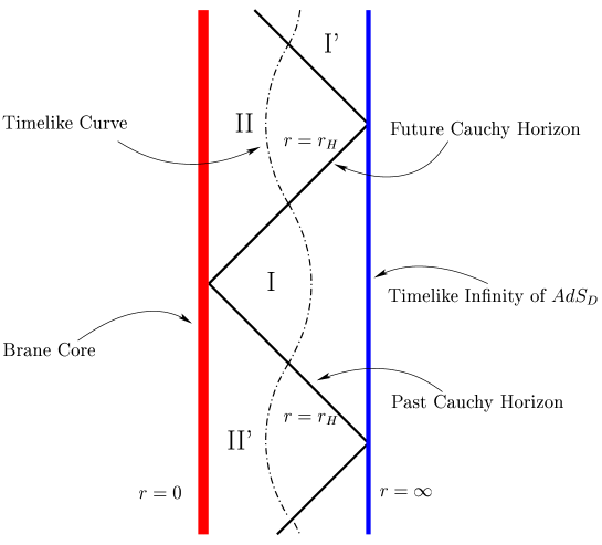
FIG. 3.: Penrose diagram for the extreme global black $p$-brane with field configurations shown in FIG. 1. The spatial coordinates $x^{i}$ and $\theta^{a}$ are suppressed. This diagram is very similar to that of the extreme Reissner-Nordström black hole, but now there is a non-singular brane core at $r=0$ rather than a curvature singularity. The boundary at $r\to\infty$ is timelike rather than null.

The near horizon geometry is very similar to that of the extreme RN black hole, of which geometry has the topology of $AdS_{2}\times S^{2}$ with constant curvature scales of $1/r_{H}$. It is easy to see that the metric (59), with $\bar{g}_{\mu\nu}(x)=\eta_{\mu\nu}$, describes a constant curvature spacetime with topology of $AdS_{p+2}\times S^{d-1}$ with curvature scales $\sqrt{(1-\alpha)^{2}B_{H}}$ and $1/r_{H}$ for $AdS_{p+2}$ and $S^{d-1}$, respectively: Components of the Riemann curvature tensor corresponding to the metric (59) are given by

$$R_{\hat{\mu}\hat{\nu}\hat{\lambda}\hat{\rho}} = -(1-\alpha)^{2}B_{H}(g_{\hat{\mu}\hat{\lambda}}g_{\hat{\nu}\hat{\rho}}-g_{\hat{\mu}\hat{\rho}}g_{\hat{\nu}\hat{\lambda}}),$$ (84)

$$R_{\theta_{a}\theta_{b}\theta_{c}\theta_{d}} = \frac{1}{r_{H}^{2}}(g_{\theta_{a}\theta_{c}}g_{\theta_{b}\theta_{d}}-g_{\theta_{a}\theta_{d}}g_{\theta_{b}\theta_{c}}),$$ (85)

where $\hat{\mu},\hat{\nu},...$ refer to $x_{\mu}$ and $r$, and $\theta_{a},\theta_{b},...$ do indices on $S^{d-1}$.

It will be helpful to rewrite the metric (59) in the form of Robinson-Bertotti (RB) metric as

$$ds^{2}_{RB}\approx\frac{\rho^{2}}{\rho_{H}^{2}}\eta_{\mu\nu}dx^{\mu}dx^{\nu}+\frac{\rho_{H}^{2}}{\rho^{2}}d\rho^{2}+r_{H}^{2}d\Omega_{d-1}^{2},$$ (86)

where we have introduced the Poincaré radial coordinate

$$\frac{\rho}{\rho_{H}}=\sqrt{B_{H}}[\sigma(r-r_{H})]^{1-\alpha}~{}~{}\Leftrightarrow~{}~{}r=r_{H}+\sigma\left(\frac{\rho}{\sqrt{B_{H}}~{}\rho_{H}}\right)^{1/(1-\alpha)},$$ (87)

with $\rho_{H}\equiv 1/\sqrt{B_{H}}(1-\alpha)$. If the radial coordinate $\rho$ ranges between $0$ and $\infty$, then the Poincaré coordinates $\{x_{\mu},\rho\}$ cover only one half of $AdS_{p+2}$, which is named as the Poincaré patch. In this coordinate system, the Cauchy horizon is at $\rho=0$ and the boundary of $AdS_{p+2}$ at $\rho=\infty$ corresponds to a $(p+1)$-dimensional flat Minkowski spacetime, $R^{1,p}$. However, with the definition Eq. (87) $\rho$ has restricted ranges and so each region covers only a part of the Poincaré patch. When $(1-\alpha)$ is positive, $\rho$ ranges from $0$ to a finite value $\rho_{f}$. For the interior solution ($\sigma=-1$), roughly $\rho_{f}\sim r_{H}^{1-\alpha}/(1-\alpha)$ (at $r\sim 0$). For the exterior region ($\sigma=1$), the metric (86) should be replaced with asymptotic solution (34) or (76) with appropriate coordinate transformation at $\rho_{f}$. Hence, with positive $(1-\alpha)$, the metric (86) describes portions including the AdS horizon of $AdS_{p+2}\times S^{d-1}$.

On the other hand, when $(1-\alpha)$ is negative, the boundary at $r=r_{H}$ is not a horizon and the metric is not that of the near horizon geometry of extremal black brane because the timelike Killing vector $\partial_{t}$ diverges at $r=r_{H}$. And, as can be observed from Eq. (83), the boundary is at a affinely infinite distance. Thus, the boundary at $r=r_{H}$ corresponds to the timelike infinity of $AdS_{p+2}$, which is conformal to flat Minkowski spacetime ${\cal M}^{1,p}$. In this branch, $\rho$ ranges from a finite value to infinity. Hence, the metric (86) describes an AdS fragment including the $(p+1)$-dimensional flat Minkowski boundary but cutting out the AdS horizon.

Recall that near the horizon of the extremal RN black hole the asymptotic metric is also written in the form of the RB metric as

$$ds_{RB}^{2}=-\frac{\rho^{2}}{r_{H}^{2}}dt^{2}+\frac{r_{H}^{2}}{\rho^{2}}d\rho^{2}+r_{H}^{2}d\Omega_{2}^{2},$$ (88)

where $r_{H}=GM$ is the size of the horizon of the extremal RN black hole. It is a kind of ‘Kaluza-Klein’ vacuum in which two directions are compactified and the ‘effective’ spacetime is the two-dimensional $AdS_{2}$ spacetime of constant negative curvature. Similarly, the $AdS_{p+2}\times S^{d-1}$ spacetime described by the near horizon metric (59) or (86) is also a ‘Kaluza-Klein’ vacuum. Usually, such type of vacuum is realized as a supersymmetric bosonic configuration, i.e., a ‘supersymmetric’ vacuum of a higher-dimensional supergravity theory. It also appears as the near horizon geometry of non-dilatonic black $p$-brane solutions of higher-dimensional supergravity or superstring theories. It will be interesting to compare the metric (59) with that of supersymmetric non-dilatonic black $p$-branes.

For comparison, we write down the metric of non-dilatonic extremal black $p$-brane:

$$ds^{2}={[\sigma\Delta(r)]}^{\frac{2}{p+1}}\eta_{\mu\nu}dx^{\mu}dx^{\nu}+\frac{dr^{2}}{{\Delta(r)}^{2}}+r^{2}d\Omega_{d-1}^{2},$$ (89)

where the extra dimension is fixed to be $d=4p/(p-1)$ and

$$\Delta(r)\equiv 1-\left(\frac{r_{H}}{r}\right)^{d-2}.$$ (90)

In the limit $r\to r_{H}$, the metric is written as

$$ds^{2} \approx \left[\frac{2(p+1)}{(p-1)r_{H}}\right]^{\frac{2}{p+1}}[\sigma(r-r_{H})]^{\frac{2}{p+1}}\eta_{\mu\nu}dx^{\mu}dx^{\nu}+\left[\frac{2(p+1)}{(p-1)r_{H}}\right]^{-2}\frac{dr^{2}}{(r-r_{H})^{2}}+r_{H}^{2}d\Omega_{d-1}^{2},$$ (91)

which explicitly has the same form as Eq. (59). Even though Eqs. (59) and (91) describe the same geometry near the horizon, the global spacetime structures of the two system, the global black brane and the non-dilatonic black brane, are much different. The spacetime of the global black brane is completely regular everywhere, whereas that of the non-dilatonic black brane is singular at the center $r=0$. The geometry of the spacetime of the global black brane asymptotes to an $AdS$ space, while that of the non-dilatonic brane does to the Minkowski spacetime.

Notice that if we used a metric ansätz using a proper radial distance instead the Schwarzschild coordinates, we would obtain a spacetime described Eq. (59) as an asymptotic solution because the horizon is sitting at infinite proper distance from the core. This is the thing done in Refs. [11] and [12], in which the authors discovered cigar-like warped spacetimes which is nothing but the infinitely long AdS throat with topology of $AdS_{p+2}\times S^{d-1}$. It is easy to see relation between the near horizon solution and the cigar-like warped spacetime obtained in Refs. [11, 12]: Introducing a new radial coordinate $\chi$($>0$) such that

$$\exp(-k\chi)\equiv\sqrt{B_{H}}~{}[\sigma(r-r_{H})]^{1-\alpha},$$ (92)

the metric Eq.(59) is rewritten as

$$ds^{2}\approx\exp\left(-2k\chi\right)\bar{g}_{\mu\nu}(x)dx^{\mu}dx^{\nu}+d\chi^{2}+r_{H}^{2}d\Omega_{d-1}^{2},$$ (93)

where the curvature scale $k$ of the $AdS_{p+2}$ is defined by $k\equiv(1-\alpha)\sqrt{B_{H}}$. For the interior solution ($\sigma=-1$), $\chi$ runs from a finite value to $\infty$ (at $r=r_{H}$). For the exterior solution ($\sigma=1$), $\chi$ runs between $\infty$ (at $r=r_{H}$) and $-\infty$ (at $r=\infty$), but $\chi$ ought to be truncated at a finite distance as, sufficiently large $r$, the near horizon geometry is replaced by the asymptotic spacetime Eq. (76). The metric (93) coincides with the cigar-like warped solution of Refs. [11, 12] in the thin core limit of $f_{H}\to 1$ where the horizon locates outside the core. Hence, among solutions obtained in [11] and [12], the meaningful solutions relevant for the Randall-Sundrum scenario would quite naturally be interpreted as the near horizon geometry of extremal global black $p$-branes. Moreover, we also find that the two solutions, Eqs. (76) and (93), which were apparently treated disjointedly in Refs. [11, 12], can be matched to each other and describe the exterior region together.

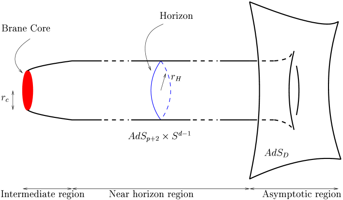
FIG. 4.: The shape of the slice of the transverse part of the spacetime of the extreme global black brane. The time and longitudinal directions are suppressed. Circles parallel to the horizon line represent $S^{d-1}$. The surface is a transversal slice.

In summary, the exterior region outside the horizon interpolates between the near horizon region, the infinitely long AdS throat with topology of $AdS_{p+2}\times S^{d-1}$, and the asymptotic region which asymptotes to $AdS_{d}$. The interior region can be divided to three separated regions, core region, near horizon region and intermediate region between the two regions. The near horizon region corresponds to the infinitely long AdS throat $(AdS_{p+2}\times S^{d-1})$. As such, the central region surrounded by the AdS throat region looks like a one-sided Randall-Sundrum domain-wall embedded in $(p+2)$-dimensional AdS spacetime $(AdS_{p+2})$. When the cosmological constant is of the same order as the fundamental scale, i.e., $M_{*}\sim|\Lambda|^{1/2}\sim M_{pl}$, most portion of the interior region is occupied by the core and near horizon regions and so the interior region is well described by only the two region. The curvature radii of both $AdS_{p+2}$ and $S^{d-1}$ are of the order of the Planck scale. At low-energy below the Planck scale, the extra space is reduced effectively to a one-dimensional space. Consequently, the global $p$-brane core looks like a $p$-dimensional domain-wall embedded in an $AdS_{p+2}$ bulk spacetime. In the ‘thin core-approximation’ limit, the system is essentially the same as that of the original Randall-Sundrum scenario. However, when the cosmological constant is much less than the fundamental scale, the core and the near horizon regions are squeezed into small portions and, in between the two most portion is occupied by an intermediate region. Since the cosmological constant is negligible in the intermediate region, its geometry can be approximated by that of the global defect spacetime in the absence of the negative cosmological constant. The geometry of this region resembles that of the Cohen-Kaplan solution [10] as $d=2$ and the global monopole solution [12] as $d\geq 3$. Putting the above results together, the spacetime geometry of the global black $p$-brane is illustrated in FIG. 4.

B Non-extreme global black branes

In this subsection we discuss the spacetime of the bent brane surrounded by two horizons, of which a field configuration is shown in FIG. 2. Since the world volume curvature of the brane core has to be positive constant, the corresponding world volume metrics are those of $(p+1)$-dimensional de Sitter spacetime, e.g.,

$$d\hat{s}^{2} = -dt^{2}+e^{2Ht}dx_{i}^{2}$$ (94)

$$= -(1-H^{2}\gamma^{2})dt^{2}+(1-H^{2}\gamma^{2})^{-1}d\gamma^{2}+\gamma^{2}d\Omega_{p-1}^{2},$$ (95)

where $\gamma^{2}\equiv x_{i}^{2}$, and $H$ is the expansion rate along the brane. The first metric (94) is defined in terms of planar coordinates and corresponds to a flat Friedman universe. The second one is static and is the analog of the Schwarzschild metric for the flat de Sitter spacetime. The $t$ in these coordinates is not the same as the $t$ in planar coordinates, but we are running out of letters. In this coordinate system $\partial_{t}$ is a Killing vector and generates the time translation symmetry. From (95), we see that at $\gamma=H^{-1}$ the norm of $\partial_{t}$ vanishes, so that it becomes null. Thus, the surface at $\gamma=H^{-1}$ is the usual de Sitter horizon. On the other hand, since $H$ is related to the world volume curvature as $\hat{R}=p(p+1)H^{2}$, from Eqs. (67) and (68) it can be read off that

$$H=\pm\frac{1}{2}e^{{A_{H}}_{\pm}}|{B_{1}}_{\pm}|.$$ (96)

The metrics (64), (65), and (71) describe only a few separated regions, but they are smoothly connected as shown in FIG. 2. Similarly to the extreme black brane case, when the cosmological constant is of the order of the fundamental scale, both the core size $r_{c}$ and the sizes of the horizons ${r_{H}}_{\pm}$ are of the order of $M_{*}^{-1}$ and so the spacetime of the interior region inside ${r_{H}}_{-}$ will be well described by the two metrics (64) and (71). On the other hand, when the cosmological constant is much less than the fundamental scale, in the intermediate region the transverse to the brane part of the solution will coincide with the metric of a global monopole of Ref. [12].

The exterior region outside the outer horizon at ${r_{H}}_{+}$ interpolates between the near horizon region and the asymptotic region described by metrics (65) and (71), respectively. In the far region, the spacetime described by the metric (65) asymptotes to $AdS_{D}$, even though the longitudinal part of the solution is not flat. The Riemann curvature tensor corresponding to the metric (65) is

$$R_{MNPQ}=\left(-B_{\infty}+\left[\frac{H^{2}}{B_{\infty}r^{2}}\right]_{M,N,P,Q\in\{x^{\mu}\}}+\left[\frac{1}{r^{2}}\right]_{M,N,P,Q\in\{\theta^{a}\}}\right)(g_{MP}g_{NQ}-g_{MQ}g_{NP}),$$ (97)

where the two terms dressed by square brackets are non-vanishing only if $M,N,P,Q\in\{x^{\mu}\}$ and $M,N,P,Q\in\{\theta^{a}\}$, respectively. Since the two terms in the square bracket decay quadratically, the spacetime asymptotes to $AdS_{D}$ as $r\to\infty$. This type of spacetime has also been found in Ref. [12], and the metric can be rewritten to the form found in Ref. [12] as done in the flat brane case

$$ds^{2}\approx e^{2\sqrt{B_{\infty}}\xi}\hat{g}_{\mu\nu}(x)dx^{\mu}dx^{\nu}+d\xi^{2}+e^{2\sqrt{B_{\infty}}\xi}d\Omega_{d-1}^{2}.$$ (98)

Now we turn to the near horizon metrics (71). One may check directly by calculating the geodesics of the metric (71) that the coordinate chart $\{x^{\mu},r,\theta^{a}\}$ is geodesically incomplete. As done in the case of flat brane, we consider the motion of test particles. It will be sufficient to consider the radial motion of test particles along the line of $\gamma=0$ in the static coordinate system to see the causal structure on the transverse slice. That is, it is sufficient to study null and timelike geodesics in the system

$$ds^{2}=-\frac{4H^{2}}{{B_{1}}_{\pm}}(r-{r_{H}}_{\pm})dt^{2}+\frac{dr^{2}}{{B_{1}}_{\pm}(r-{r_{H}}_{\pm})},$$ (99)

where we have used the relation (96). This metric is reminiscent of the near horizon metrics of the non-extremal Reissner-Nordström black hole. The proper distances from a point $r_{0}$ to the horizons in a constant time slice is finite and is given by $\chi(r_{0})\sim 2\sqrt{(r_{0}-{r_{H}}_{\pm})/{B_{1}}_{\pm}}$. With this metric we find the geodesic equation

$$\kappa=-\frac{H^{2}}{{B_{1}}_{\pm}}(r-{r_{H}}_{\pm})\left(\frac{dt}{d\tau}\right)^{2}+\frac{1}{{B_{1}}_{\pm}(r-{r_{H}}_{\pm})}\left(\frac{dr}{d\tau}\right)^{2}.$$ (100)

With the static world volume metric, there is a constant of motion corresponding to the Killing vector $\partial_{t}$

$$\epsilon=\frac{H^{2}}{{B_{1}}_{\pm}}(r-{r_{H}}_{\pm})\frac{dt}{d\tau}.$$ (101)

The equation of motion of the test particles then is

$$\left(\frac{dr}{d\tau}\right)^{2}-\epsilon^{2}\frac{{B_{1}}_{\pm}}{H^{2}}-\kappa{B_{1}}_{\pm}(r-{r_{H}}_{\pm})=0.$$ (102)

The equation of motion tells that the test particle reach at the horizon with a finite velocity, i.e., $(dr/d\tau)\to\epsilon{B_{1}}_{\pm}/H$ as $r\to{r_{H}}_{\pm}$. Therefore, the coordinate chart $\{x^{\mu},r,\theta^{a}\}$ is geodesically incomplete and so the extensions beyond each horizon are required. If the solutions obtained in separated regions are mutually connected as shown in FIG. 2, the causal structure induced by the $(t,r)$-part of the solutions will resemble that of the non-extreme RN black hole. The differences are the non-singular brane core instead a curvature singularity at $r=0$ and the timelike boundary rather than null at $r=\infty$. The corresponding Penrose diagram is shown in FIG. 5.

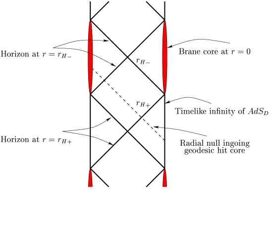
FIG. 5.: Penrose diagram for the non-extreme global black brane with field configurations shown in FIG. 2. The spatial coordinates $x^{i}$ and $\theta^{a}$ are suppressed. This diagram is very similar to that of the non-extreme Reissner-Nordström black hole, but now there is a non-singular brane core at $r=0$ rather than a curvature singularity. The boundary at $r=\infty$ is timelike rather than null.

The metric (71) has some very interesting properties. The metrics with the form of (71) usually have curvature singularities at $r={r_{H}}_{\pm}$. However, when the relation (96) holds, the curvature invariants are finite and the surfaces at $r={r_{H}}_{\pm}$ do indeed appear to be just coordinate singularities. For example, the corresponding Kretschmann scalar near each horizon at $r={r_{H}}_{\pm}$ is given by

$$R_{MNPQ}R^{MNPQ}=\frac{2(d-1)(d-2)}{{r_{H}}_{\pm}^{4}}.$$ (103)

This is not surprising, since the metric (71), in fact, describes constant curvature spacetimes with topology of locally $(p+2)$-dimensional flat Minkowski spacetime multiplied by $(d-1)$-dimensional sphere with radius ${r_{H}}_{\pm}$, i.e., ${\cal M}^{1,p+1}\times S^{d-1}$. This can easily be observed by calculating the Riemann curvature tensor and noticing that the only non-vanishing components of the corresponding Riemann curvature tensor are

$$R_{\theta_{a}\theta_{b}\theta_{c}\theta_{d}}=\frac{1}{{r_{H}}_{\pm}^{2}}(g_{\theta_{a}\theta_{c}}g_{\theta_{b}\theta_{d}}-g_{\theta_{a}\theta_{d}}g_{\theta_{b}\theta_{c}}),$$ (104)

where $\theta_{a},\theta_{b},...$ refer to indices on $S^{d-1}$.

It is interesting to observe that the $(p+2)$-dimensional flat part corresponds the spacetime of a $p$-dimensional thin domain wall embedded in $(p+2)$-dimensional flat spacetime, which is a generalization of the inflating three-brane in four-dimensions [23]. The metric (71) can be rewritten to an analogous form to that of the inflating three-brane found in Ref. [23] introducing a new radial coordinate $e^{-2Hz}\equiv 4H^{2}[(r-{r_{H}}_{\pm})/{B_{1}}_{\pm}]$, the metric can easily be rewritten as

$$ds^{2}=e^{-2Hz}\left[d\hat{s}^{2}+dz^{2}\right]+{r_{H}}_{\pm}^{2}d\Omega_{d-1}^{2},$$ (105)

where the horizons are located at $z=\infty$. Another coordinate transformation $\rho\equiv 2\sqrt{{B_{1}}_{\pm}(r-{r_{H}}_{\pm})}/{B_{1}}_{\pm}+\rho_{0}$, where $\rho_{0}$ is an integral constant, brings Eq. (71) to the form

$$ds^{2}=(1-H\rho)^{2}d\hat{s}^{2}+d\rho^{2}+{r_{H}}_{\pm}^{2}d\Omega_{d-1}^{2},$$ (106)

where the relation Eq. (96) has been used and $\rho_{0}$ has been set as to be $\rho_{0}=H^{-1}$, so that the horizons are at $\rho=H^{-1}$. The $(x_{\mu},\rho)$-parts of metrics explicitly coincide with those of the vacuum domain wall obtained in Ref. [23]. Thus, the near horizon spacetime of the bent brane is nothing but that of $(p+2)$-dimensional vacuum domain wall times $(d-1)$-dimensional sphere.

The spacetime of domain walls has been extensively studied in many literatures [23, 24, 25, 26, 27, 28, 29, 30, 31, 32]. For the metric Eq. (105), the $z={\rm const}$ (or $\rho={\rm const}$ for Eq. (106)) hypersurfaces have the properties of $(p+1)$-dimensional de Sitter space. Furthermore, the $(t,z)$-part (or $(t,\rho)$-part) of the metric describes a $(1+1)$-dimensional Rindler space (i.e., flat space in the reference frame of a uniformly accelerating observer with proper acceleration $H$). Therefore, at each of the $(p+1)$ spatial directions event horizons exist. The ones in the $p$ longitudinal directions are de Sitter-like as discussed at the beginning of this subsection. The one in the radial direction is Rindler-like, and the various extensions beyond it were considered in Refs. [23, 25, 27]. The extensions could be simply obtained by gluing together two portions of Minkowski spacetime. Such extensions occupy only the interior region of the Penrose diagram of FIG. 5 without the exterior region interpolating between the horizon and the timelike infinity. On the other hand, the global spacetime of non-extreme global black brane corresponding to the field configuration of FIG. 2 bears remarkable similarities to that of the non-extreme domain walls found in Ref. [30].

When the horizon size ${r_{H}}_{-}$ is of the order of the Planck length scale (this will be true if $|\Lambda|^{1/2}\sim M_{*}\sim M_{pl}$), at low-energy below the Planck scale the brane core will look like a inflating domain wall embedded in $(p+2)$-dimensional Minkowski spacetime to an observer residing near the inner horizon. However, when the bulk cosmological constant is much less than the fundamental scale, the horizon size is much larger than the fundamental length scale and so, even at low-energy, the core will look like a string, or a monopole, etc, depending on the number of extra dimensions rather than a domain wall. Interestingly, when $p=1$ and $d=2$ the metric (106) itself coincide with the asymptotic solution near the horizon of the non-static global cosmic string found in Ref. [5], and the interior region inside the inner horizon resembles the spacetime of the non-static global cosmic string. On the other hand, the nature of the cosmological event horizon of Refs. [5, 6] seems to be different from the inner horizon at ${r_{H}}_{-}$, in the sense that across the cosmological event horizon the coordinates $t$ and $\rho$ of [5, 6] remain timelike and spacelike respectively, while the roles of $t$ and $\rho$ in the metric (106) is exchanged across the inner horizon. The interior region of the other defects of $p>1$ and $d\geq 2$ are simply the generalizations of the non-static global cosmic string spacetime.

V Brane worlds and a thermal instability for the cosmological constant

In this section we consider the global black branes as an approximation for brane world scenarios. We will shortly summarize the contents of Ref. [16], in which the extremal ones only are considered, and discuss the effective gravity on the brane when it is non-extremal. We briefly comment a few thermodynamic properties of the global black branes, and discuss a decrease of the effective cosmological constant in the brane world through thermal instability of the non-extremal black brane. The exterior region of the extremal global black branes by itself does not seem to provide a suitable framework for the brane world scenario, because in one direction one will reach the $(p+2)$-dimensional AdS horizon, while in the other direction one will reach the $D$-dimensional AdS spacetime. On the other hand, the interior region possesses all the feature necessary for realizing the Randall-Sundrum (RS) type brane world scenario. In one direction, it asymptotes to the infinitely long AdS throat. As such, the central region surrounded by the AdS region looks like a one-sided RS domain-wall embedded in $(AdS_{p+2})$. As discussed in Ref. [16], the size of the horizon can be interpreted as the effective size of $d$ extra dimensions in that the Planck scale in the $p$-dimensional brane world $M_{pl}$ is determined by the fundamental scale $M_{*}$ and the horizon size $r_{H}$ via the familiar relation $M_{pl}^{p-1}\sim M_{*}^{p-1+d}r_{H}^{d}$. Moreover, the gravity on the brane world behaves as expected in a world with $d$-extra dimensions compactified with size $r_{H}$.

When the fundamental scale and the bulk cosmological constant are of the order of the brane world Planck scale, i.e., $M_{*}\sim|\Lambda|^{1/2}\sim M_{pl}$, then the curvature radii of $AdS_{p+2}$ and $S^{d-1}$ are of the order of the Planck scale. Thus, at low-energy below the Planck scale, the extra space is reduced effectively to a one-dimensional space. Consequently, the global $p$-brane core looks like a $p$-dimensional domain-wall embedded in an $AdS_{p+2}$ bulk spacetime. In the ‘thin core-approximation’ limit, the physics on the brane is essentially the same as that of the original RS scenario. On the other hand, when the cosmological constant is hierarchically smaller than the fundamental mass scale, the horizon size is much larger than the core size or the fundamental length scale, i.e., $r_{H}\gg r_{c}\sim M_{*}^{-1}$, so the physics is quit analogous to that of the large extra dimension scenario. Then the Planck scale $M_{pl}$ in the brane world is hierarchically bigger than the fundamental scale $M_{*}$ of the higher dimensional gravity, according to the familiar relation $M_{pl}^{p-1}\sim M_{*}^{p-1+d}r_{H}^{d}$. And as shown in Ref. [16], the phenomenology on the brane is imperceptibly different from that of the usual large extra dimension scenario.

For the bent branes surrounded by two horizons, since the interior region is bounded by the inner horizon as the interior region of the extreme black brane is bounded by the Cauchy horizon, the outside of the inner horizon is out of causal contact with the brane world. So the Planck scale on the brane world is given by $M_{pl}^{p-1}\sim M_{*}^{p-1+d}{r_{H}}_{-}^{d}$. The interior region has similar features to the inflating domain wall spacetime or the de Sitter brane, so the gravity on the brane will resemble that on the de Sitter brane. As discussed in Refs. [34, 35, 36], the massless graviton is trapped on the de Sitter brane reproducing the correct $(p+1)$-dimensional gravity on the brane as on the Minkowski brane. A difference is that in the Minkowski case the massless graviton is a marginal bound state and the continuum of Kaluza-Klein modes starts at zero mass, while in the de Sitter case the graviton is separated by a finite mass gap of $m=(3/2)H$ from the continuum, that is, the Kaluza-Klein continuum modes starts at $m=(3/2)H$.

In this picture, the Hawking radiation could be a possible mechanism for the resolution of various problems associated with the brane world scenarios, such as the observed flatness and the approximate Lorentz invariance of our world. The bending of the brane and the bulk curvature that violate the $SO(3,1)$ isometry on our brane [37, 38] would correspond to excitations upon the extremal state, and the excited states that correspond to non-extremal states would evolve into an extremal state through the Hawking radiation process. The similar argument may be applicable as well for the cosmological constant problems.

We now turn to the thermal instability of the non-extremal black branes, which could be a mechanism resolving the cosmological constant problem. In the brane world, the intrinsic curvature of the brane amounts to a net cosmological constant as viewed by an observer pinned on the brane, i.e., $\Lambda_{\rm phys}=[(p-1)/2(p+1)]\hat{R}$. Since we have found that, in higher-dimensional pure gravity theory with a cosmological constant term $\Lambda$ explicitly, there exists a class of solutions with physical $(p+1)$-dimensional metrics obeying the standard Einstein equations with positive arbitrary (including zero) values of $\Lambda_{\rm phys}$ or $\hat{R}$, the cosmological constant problem may be solved by choosing a solution characterized by vanishingly small $\Lambda_{\rm phys}$, that is, a very near extremal black brane solution. However, this doesn’t seem to tell anything about the cosmological constant problem, because there are no convincing arguments in favor of this choice. In this respect, we might need a dynamical mechanism that singles out the solution with an extremely small $\Lambda_{\rm phys}$, which would be a complete solution to the cosmological constant problem. As discussed in Refs. [16, 18], a possible dynamical mechanism may be related to the thermodynamic instability of the non-extreme black branes, by which the positive vacuum energy density on the brane could be radiated away causing the brane to evolve into an extremal state.

In this respect, we briefly comment a few thermodynamic properties of the extreme and non-extreme global black branes, and discuss a decrease of the effective cosmological constant on the brane. For the extremal black brane, since the surface gravity is zero at the degenerated horizon, the Hawking temperature is zero and there is no Hawking radiation. Thus, this system is in fact thermodynamically stable. The entropy of a system is associated with the number of accessible states. Since the extremal state of the global black brane seems to be a unique solution to the equations of motion as discussed in the subsection III A, its entropy would be zero. On the other hand, the entropy associated with a spacetime containing horizon is given by the area of the event horizon: $S_{BH}=A_{D}/4\pi G_{D}$, where $A_{D}$ is the area of the horizon and $G_{D}$ is the $D$-dimensional Newton constant. The area of the spacelike surface of constant $r$ reads from the metric Eq.(59) as: $A_{D}(r)\sim(r-r_{H})^{2p(1-\alpha)}$, which clearly vanishes as $r\to r_{H}$. This supports the conclusion of zero entropy property of the extreme black brane.

For the non-extremal case, as mentioned in the previous section there are de Sitter horizon in $p$ longitudinal directions and the Rindler horizon in radial direction. The de Sitter horizon is associated with a surface gravity $\kappa=H$ and so an observer will detect an isotropic background in the longitudinal directions of thermal radiation with temperature $T=(2\pi)^{-1}H$ coming, apparently, from the horizon [33]. The de Sitter horizon also may be interpreted as the entropy or lack of information that the observer has about the regions of the universe that he cannot see. If one absorbs the thermal radiations, one gains energy and entropy at the expanse of this region and so the area of the horizon will go down according to the first law of the black hole dynamics. As the area decreases, the temperature of the cosmological radiation goes up (like the black hole case), so the cosmological event horizon is unstable. On the other hand, at the Rindler horizon the surface gravity can be identified by the proper acceleration of a uniformly accelerating observer. Since the metric corresponds to that of the uniformly accelerating observer with the proper acceleration $H$, the surface gravity is simply given by $\kappa=H$, and the temperature measured by a static observer near both horizons at ${r_{H}}_{\pm}$ is just $T=(2\pi)^{-1}H$ or $T=(2\pi)^{-1}\sqrt{2\Lambda_{\rm phys}/p(p-1)}$. Therefore, the observer will detect two thermal radiations with the same temperatures of $T=(2\pi)^{-1}H$ coming from the de Sitter horizon and the Rindler one, respectively. This seems to be well matched with the zeroth law of black hole mechanics. Here, an interesting point is that the surface gravity at the horizons is determined by the brane world volume curvature solely regardless the size of the horizon unlike usual black hole and static black brane cases. An observer residing in the exterior region at a distance from the outer horizon may observe a steady current of thermal radiation coming from the outer horizon and going out toward the asymptotically anti-de Sitter infinity, even if the observer see an isotropic thermal background in the longitudinal directions. This implies a possibility that the non-extreme black brane could evolve into an extreme black brane of which world volume is flat. Since the brane itself is the source of the radiation in radial direction, this must result in energy loss from the brane. If the quantum fluctuations of the vacuum energy on the brane is coupled to bulk fields (including bulk gravitational field), then the vacuum energy density could be radiated into the bulk outside of the outer horizon through the Hawking radiation process, resulting in a decrease of the vacuum energy density or, equivalently, the world volume curvature $\hat{R}$. Thus, the Hawking temperature goes down with time, and the radiation will last until the temperature reaches to zero. Since the temperature is proportional to $\sqrt{\hat{R}}$, the radiation will go on until $\hat{R}=0$. Equivaletly, since the temperature is proportional to the square root of the effective cosmological constant, $\sqrt{\Lambda_{\rm phys}}$, the radiation will continue until $\Lambda_{\rm phys}=0$. Thus, this effect may radiate away all contributions to the cosmological constant.

VI Conclusions

In this paper we have mainly examined global black $p$-brane solutions, which are black hole-like $p$-dimensional extended global defect solutions to a scalar theory with global $O(d)$ internal symmetry coupled to higher-dimensional gravity with a negative cosmological constant. The spacetimes of them are perfectly regular everywhere. We have found series solutions in a few separated regions and numerically showed that they can be smoothly connected. There are two kinds of such solutions, extremal or non-extremal black branes. The extremal black branes have a Ricci flat world volume and are surrounded by a degenerated Killing horizon. On the other hand, the world volumes of non-extremal black branes surrounded by two horizons are not Ricci flat but of non-zero constant curvature. The extremal black brane solutions seem to be the critical limit of non-extremal ones, in that the positions of two horizons of non-extremal branes approach to and are degenerated at the position the horizon of extremal black branes in the limit that the world volume curvature goes to zero, i.e., $\hat{R}\to 0$. The exterior region of both objects asymptotes to anti-de Sitter infinity.

The near horizon geometries of both the extremal and the non-extremal branes have very interesting features. For the extremal black brane the geometry is the infinitely long anti-de Sitter throat with the topology of $AdS_{p+2}\times S^{d-1}$. The curvature scales of both $AdS_{p+2}$ and $S^{d-1}$ parts are of the order of $\sqrt{|\Lambda|}$. So the core will look like a one-side flat domain wall embedded in $(p+2)$-dimensional anti-de Sitter space to an observer residing in the near horizon region of the interior region if the size of the sphere is small so that the observer doesn’t see $S^{d-1}$-part. The physics on the branes then is essentially the same as that on the Randall-Sundrum brane as discussed in Ref. [16]. On the other hand, for the non-extremal ones it is the $(p+2)$-dimensional flat spacetime times $(d-1)$-dimensional sphere with radii ${r_{H}}_{\pm}$ at each horizon. The $(p+2)$-dimensional flat part corresponds to the spacetime of a $p$-dimensional thin domain wall embedded in $(p+2)$-dimensional flat spacetime. An observer residing in the near horizon region inside the inner horizon will see an inflating domain wall if the size of the inner horizon is small enough. Therefore, the gravitational Kaluza-Klein modes have a mass gap in the spectrum and the continuous spectrum starts above the mass $m=(3/2)H$, where $H$ is the expansion rate of the brane.

In the brane world, the world volume curvature amounts to the effective cosmological constant. We obtained a flat brane solution with $\hat{R}=0$ (i.e., the extremal black brane) without fine-tuning between parameters in the Lagrangian. However, to solve the cosmological constant problem completely we need a dynamical mechanism that picks out the flat brane solution among whole solutions of any $\hat{R}$. We have suggested a possible thermodynamic mechanism as a candidate for such mechanism. It is provable for a non-extremal black brane to evolve into an extremal black brane owing to its thermodynamic instability. It might emit a thermal radiation with temperature $T\propto\sqrt{\hat{R}}\propto\sqrt{\Lambda_{\rm phys}}$ resulting in a decrease of the vacuum energy on the brane, flattening itself and finally reaching to the extremal limit at temperature $T=0$. This effect will dilute all contribution to the cosmological constant. If it is really possible, then the black brane world model represents a solution to the cosmological constant problem.

REFERENCES

- [1] A. Vilenkin and E.P.S. Shellard, Cosmic String and other Topological Defects, Cambridge University Press, 1994.
- [2] R. Gregory, Phys. Lett. B 215, 663 (1988); G.W. Gibbons, M.E. Ortiz and F. Ruiz-Ruiz, Phys. Rev. D 39, 1546 (1989).
- [3] A. G. Cohen and D. B. Kaplan, Phys. Lett. B 215, 67 (1988).
- [4] M. Barriola and A. Vilenkin, Phys. Rev. Lett. 63, 341 (1989).
- [5] R. Gregory, Phys. Rev. D 54, 4955 (1996).
- [6] A. Wang and J.A.C. Nogales, Phys. Rev. D 56, 6217 (1997).
- [7] N. Arkani-Hamed, S. Dimopoulos and G. Dvali, Phys. Lett. B429 (1998) 263; Phys. Rev. D 59 (1999) 086004;
- [8] L. Randall and R. Sundrum, Phys. Rev. Lett. 83, 3370 (1999).
- [9] L. Randall and R. Sundrum, Phys. Rev. Lett. 83, 4690 (1999).
- [10] A. G. Cohen and D. B. Kaplan, Phys. Lett. B 470, 52 (1999).
- [11] R. Gregory, Phys. Rev. Lett. 84, 2564 (2000).
- [12] I. Olasagati and A. Vilenkin, Phys. Rev. D 62, 044014 (2000).
- [13] T. Gherghetta and M. Shaposhnikov, Phys. Rev. Lett. 85, 240 (2000).
- [14] T. Gherghetta, E. Roessl and M. Shaposhnikov, Phys. Lett. B 491, 353 (2000).
- [15] I. Oda, Phys.Lett. B 496, 113 (2000).
- [16] Y. Kim, S.-H. Moon and S.-J. Rey, Nucl. Phys. B 602, 467 (2001).
- [17] K. Benson and I. Cho, Phys. Rev. D 64, 065026 (2001).
- [18] W.S. Bae, Y.M. Cho and S.-H. Moon, J. High-Energy Phys. 0103, 039 (2001).
- [19] N. Kim, Y. Kim and K. Kimm, Phys. Rev. D 56, 8029 (1997); Class. Quant. Grav. 15, 1513 (1998).
- [20] Y. Kim and S.-H. Moon, Phys. Rev. D 58, 105013 (1998); G. Clément and A. Fabbri, Class. Quant. Grav. 17, 2537 (2000).
- [21] K. Lee, V.P. Nair and E.J. Weinberg, Phys. Rev. Lett. 68, 1100 (1992); Phys. Rev. D 45, 2751 (1992).
- [22] G.T. Horowitz and A. Strominger, Nucl. Phys. B 360, 197 (1991).
- [23] A. Vilenkin, Phys. Lett. B 133, 177 (1983).
- [24] L.M. Widrow, Phys. Rev. D 39, 3571 (1989).
- [25] G.W. Gibbons, Nucl. Phys. B 394, 3 (1993).
- [26] A. Wang and P.S. Letelier, Phys. Rev. D 51, R6612 (1995).
- [27] A. Wang and P.S. Letelier, Phys. Rev. D 52, 1800 (1995).
- [28] M. Cvetic, S. Griffies and S.-J. Rey, Nucl. Phys. B 381, 301 (1992); Nucl. Phys. B 389, 3 (1993).
- [29] M. Cvetic, R.L. Davis, S. Griffies, and H.H. Soleng, Phys. Rev. Lett. 70, 1191 (1993).
- [30] M. Cvetic, S. Griffies, and H.H. Soleng, Phys. Rev. Lett. 71, 670 (1993).
- [31] N. Kaloper and A. Linde, Phys. Rev. D 59, 101303 (1999).
- [32] N. Kaloper, Phys. Rev. D 60, 123506 (1999).
- [33] G.W. Gibbons and S.W. Hawking, Phys. Rev. D 15, 2738 (1977).
- [34] O. DeWolfe, D.Z. Freedman, S.S. Gubser, and A. Karch, Phys. Rev. D 62, 046008 (2000).
- [35] A. Karch and L. Randall, J. High-Energy Phys. 0105, 008 (2001).
- [36] J. Garriga and M. Sasaki, Phys. Rev. D 62, 043523 (2000).
- [37] D.J.H. Chung, E.W. Kolb, and A. Riotto, Extra dimensions present a new flatness problem, hep-ph/0008126.
- [38] J.F. Vázquez-Poritz, Massive Gravity on a Non-extremal Brane, hep-th/0110299.
- [39] V.A. Rubakov and M.E. Shaposhnikov, Phys. Lett. B 125 (1983) 139.
- [40] N. Arkani-Hamed, S. Dimopoulos, N. Kaloper, and R. Sundrum, Phys. Lett. B 480, 193 (2000).
- [41] S. Kachru, M. Schulz, and E. Silverstein, Phys. Rev. D 62, 045021 (2000).
- [42] A. Kenhagias and K. Tamvaski, A Self-Tuning Solution of the Cosmological Constant Problem, hep-th/0011006.
- [43] N. Tetradis, Phys. Lett. B 509, 307 (2001).
- [44] J.E. Kim, B. Kyae and H.M. Lee, Phys. Rev. Lett. 86, 4223 (2001); Nucl. Phys. B 613, 306 (2000).
- [45] S. Forste, Z. Lalak, S. Lavignac, and H.P. Nilles, Phys. Lett. B 481, 360 (2000); J. High-Energy Phys. 0009, 034 (2000).
- [46] C. Csaki, J. Erlich, C. Grojean, and T. Hollowood, Nucl. Phys. B 584, 359 (2000).
- [47] I. Low and A. Zee, Nucl. Phys. B 585, 395 (2000).
- [48] P. Binetruy, J.M. Cline and C. Grojean, Phys. Lett. B 489, 403 (2000).
- [49] J. Diemand, C. Mathys and D. Wyler, Dynamical Instabilities of Brane World Models, hep-th/0105240.
- [50] A.J.M. Medved, Dynamical Instability of Self-Tuning Solution with Antisymmetric Tensor Field, hep-th/0109180.
- [51] N. Bahcall, J.P. Ostriker, S. Perlmutter and P.J. Steinhardt, Science 284, 1481 (1999).
- [52] S. Alexander, Yi Ling, and Lee Smolin, A thermal instability for positive brane cosmological constant in the Randall-Sundrum cosmologies, hep-th/0106097.