SU-ITP 01-52

hep-th/0112081

Open Dielectric Branes

Mark Van Raamsdonk

Institute for Theoretical Physics

Stanford University

Stanford, CA, 94306 U.S.A

mav@itp.stanford.edu

We derive leading terms in the effective actions describing the coupling of bulk supergravity fields to systems of arbitrary numbers of Dp-branes and D(p+4)-branes in type IIA/IIB string theory. We use these actions to investigate the physics of Dp-D(p+4) systems in the presence of weak background fields. In particular, we construct various solutions describing collections of Dp-branes blown up into open D(p+2)-branes ending on D(p+4)- branes. The configurations are stabilized by the presence of background fields and represent an open-brane analogue of the Myers dielectric effect. To deduce the D-brane actions, we use supersymmetry to derive operators corresponding to moments of various conserved currents in the Berkooz-Douglas matrix model of M-theory in the presence of longitudinal M5-branes and then use dualities to relate these operators to the worldvolume operators appearing in the Dp-D(p+4)-brane effective actions.

December 2001

1 Introduction

One of the most remarkable properties of D-branes in string theory is that while a single Dp-brane behaves geometrically much like a classical p-dimensional surface, collections of many Dp-branes can exist in configurations completely different from those of a set of such classical surfaces. For example, configurations of $N$ D0-branes with coordinate matrices that do not mutually commute do not have well defined positions for the D0-branes [1]. In some cases, the interpretation as a set of $N$ particles is lost entirely, and the configuration of D0-branes is better described as a smooth, higher dimensional object.

A standard example is the fuzzy sphere [2, 3] for which the first three coordinate matrices for a set of $N$ D0-branes are identified with the generators of the $N$-dimensional irreducible representation of $SU(2)$, $X^{i}=\alpha J^{i}$. This configuration, for which

$$[X^{i},X^{j}]=\alpha i\epsilon^{ijk}X^{k}\;,$$ (1)

has an alternate description as a spherical D2-brane of radius $R\approx{\alpha N\over 2}$ with a uniform magnetic field on its worldvolume (corresponding to the zero-brane charge). A second example, with an infinite number of D0-branes, is given by choosing $X^{i}$ such that

$$[X^{i},X^{j}]=i\theta^{ij}\;$$

for constant $\theta$ [4]. In this configuration, the coordinate matrices represent the algebra of noncommutative $R^{2n}$ and the physical interpretation is an infinite flat D(2n)-brane with a uniform magnetic field $F_{12}=\dots=F_{(2n-1)\;(2n)}$. This ability to construct higher dimensional brane configurations using D0-branes is essential for the success of the BFSS Matrix Theory [5], where for example arbitrary membrane configurations in M-theory must be described in terms of the low energy degrees of freedom of D0-branes.

The examples above indicate that while noncommuting configurations do not have well defined positions for the individual D0-branes, there is still some geometrical interpretation. In fact, it is still possible to measure the spacetime distribution of matter and charges for an arbitrary noncommuting configuration using the operators coupling to bulk supergravity fields in the low energy effective action. For example, the zero-brane charge distribution is measured by the operator coupling to the time component of the Ramond-Ramond one-form field, and is given (at weak coupling and small $\alpha^{\prime}$) in momentum space by [6]

$${\cal J}_{(1)}^{0}(k)={\rm Tr}\,(e^{ik\cdot X})\;.$$ (2)

Operators measuring multipole moments of the zero-brane charge distribution correspond to derivatives with respect to $k$ of this expression at $k=0$. Similarly, the D(2p+1)-brane charge density is measured by operators

$${\cal J}_{(2n+1)}^{0i_{1}\cdots i_{2n}}(k)\propto{\rm STr}\,([X^{[i_{1}},X^{i_{2}}]\cdots[X^{i_{2n-1}},X^{i_{2n}]}]e^{ik\cdot X})$$ (3)

coupling to the higher Ramond-Ramond fields in the effective action. From this expression it is manifest that noncommuting configurations of D0-branes involve higher dimensional brane charges. These operators and the corresponding bulk-brane effective actions (for weak coupling and small $\alpha^{\prime}$) were worked out for D0-branes in [6] and for Dp-branes of any dimension in [7, 8].

Of course, these effective actions also permit the study of collections of D-branes in the presence of weak background fields, and in particular provide a method to produce stable noncommutative brane configurations with higher dimensional brane charges. For example, Myers showed that in the presence of a constant Ramond-Ramond three-form field strength, a system of D0-branes will blow up into the spherical D2-brane configuration (1) with a radius proportional to the field strength [8].

Thus, the low energy effective actions describing linear couplings of bulk supergravity fields to the D-brane worldvolume fields provide essential tools in understanding the spacetime properties of general noncommuting D-brane configurations.

Open branes

So far, we have discussed collections of a single type of D-brane in the bulk, and the higher dimensional branes that arose from noncommuting configurations were “closed” branes in the sense that they have the geometry of surfaces without boundaries, and carry zero net higher dimensional brane charges in the case of finite $N$ (due to the vanishing of the expressions (3) at $k=0$). On the other hand, it is well known that branes can often have boundaries on higher dimensional branes [9]. Perhaps the simplest example is that a Dp-brane can end on D(p+2)-brane (related by S and T-duality to the fact that fundamental strings may end on D-branes). Given that D-branes can exist in higher dimensional closed brane configurations, it is natural to ask whether we can also build open brane configurations from lower dimensional branes. For example, can we find configurations of Dp-branes corresponding to open D(p+2)-branes ending on D(p+4)-branes?

A hint that the answer is yes is provided by the matrix model of Berkooz and Douglas, proposed to describe M-theory in the presence of longitudinal M5-branes [10] (see also [11]). If correct, this model should include states corresponding to arbitrarily shaped open membranes ending on the M5-branes, since these open membranes are allowed objects in M-theory. On the other hand, the degrees of freedom of the model are the lowest energy modes of 0-0 strings and 0-4 strings in a system of $N$ D0-branes and $k$ D4-branes, where $N$ represents the DLCQ momentum in the theory and $k$ corresponds to the number of $M5$-branes. Thus, we should be able to describe arbitrary open membranes in terms of the degrees of freedom of D0-branes in the presence of D4-branes. Interpreted in the context of type IIA string theory at low energies and weak coupling, these configurations should correspond to D0-branes blown up into open D2-branes ending on the D4-branes.

In this paper, motivated by the Berkooz-Douglas matrix model, we will consider systems of Dp-branes in the presence of D(p+4)-branes and look for classical configurations in which the Dp-branes form a noncommutative open D(p+2)-brane ending on the D(p+4)-branes. Just as for the case of noncommutative closed-brane configurations, an essential tool will be the low energy effective action describing the couplings of the brane system to the bulk supergravity fields. Since this effective action has not to our knowledge been determined previously for the Dp-D(p+4) system with arbitrary number of Dp-branes and D(p+4) branes, our first task will be to provide a derivation of some of the leading terms in this action.

Thus, the goals of this paper will be to derive leading terms in the effective action describing the couplings of the Dp-D(p+4) system to bulk supergravity fields and to use this effective action to create and study open noncommutative branes.

A summary of the remainder of the paper is as follows. In section 2, we discuss various tools that will be useful in constructing the Dp-D(p+4) effective actions. We recall that all the actions are related by T-duality and further that these actions are related to the action for Matrix theory (in this case, the Berkooz-Douglas matrix model) in the presence of background 11-dimensional supergravity fields. We will find it simplest to derive the currents in the matrix model. In section 3, we show that all the currents are related to each other by supersymmetry and that in the matrix model context, these supersymmetry relations may be used to derive all the currents from a single “primary” current, namely the operator $T^{++}$ coupling to the metric component $h_{++}$ (corresponding in the D0-D4 picture to the zero-brane density $J_{0}$). In section 4, as a check of our approach, we use these supersymmetry relations in the context of the BFSS matrix model to rederive the currents for systems of a single type of D-brane starting from the expression (2). We find complete agreement with known expressions for the matrix theory currents derived in [13, 14, 15].

In section 5, we recall the Berkooz-Douglas matrix model, obtained from the dimensional reduction of the D5-D9 action in flat space. In section 6, we use our supersymmetry relations to derive leading terms in the operators describing conserved currents in the Berkooz-Douglas model. In this case, we do not even know the “primary” operator $T^{++}$ except that it should agree with the BFSS result (2) when the fields arising from 0-4 strings are set to zero. Nevertheless, we are able to deduce the leading new terms (quadratic in the 0-4 strings) by demanding consistency of the supersymmetry relations. This is enough to determine leading operators in the Dp-D(p+4) actions coupling to arbitrary weak type II supergravity fields, and we present these results in section 7.

In section 8, we apply our results to look for noncommutative open-brane configurations. We first discuss configurations of D0-branes corresponding to flat open D2-branes of various shapes inside a D4-brane. In particular, we show explicitly that planar configurations of noncommutative instantons carry non-zero D2-brane area, as suggested previously by Berkooz in the context of the matrix model for the noncommutative (0,2) theory [12]. Since these instanton configurations are supersymmetric, we may conclude that the flat noncommutative D2-brane solutions we discuss are stable and BPS. Starting from a disk-like open D2-brane configurations, we show that by turning on a gradient of either the RR one-form or the RR three-form potential in a direction perpendicular to the D4-brane, we can pull the interior of the open D2-brane off the D4-brane such that the final configuration is a bulging parabolic D2-brane with a circular boundary on the D4-brane (for a preview, see figure 6 in section 8.4). Thus, starting with a collection of coincident D0-branes, we can turn on a combination of background fields to produce an “open dielectric brane” analogous to closed dielectric brane discovered by Myers.

In section 9, we discuss an approach based on the ADHM construction for deriving higher order terms in the expression for the primary current $T^{++}$ in the Berkooz-Douglas model that would allow a more complete derivation of the Dp-D(p+4) effective actions. Finally, we offer some concluding remarks in section 10 and a variety of useful formulae and results in a set of appendices.

2 Deriving D-brane actions

We would like to derive leading terms in the effective actions describing the couplings of type IIA/IIB supergravity fields to the worldvolume fields of a system of Dp-branes and D(p+4)-branes. These worldvolume fields arise from the massless excitations of open p-p strings, p-(p+4) strings, and (p+4)-(p+4) strings. The (p+4)-(p+4) fields propagate on the (p+5)-dimensional worldvolume of the D(p+4)-branes, while the p-p and p-(p+4) fields are restricted to the (p+1)-dimensional worldvolume of the Dp-branes. The field content and flat space Lagrangian of the theory will be reviewed in section 5.

In general, the effective action for the couplings of type II supergravity fields to the worldvolume fields on a system of D-branes takes the form

$$S=\int d^{10}x({1\over 2}h_{\mu\nu}{\cal T}^{\mu\nu}+\phi{\cal J}_{\phi}+{1\over 2}B_{\mu\nu}{\cal J}_{s}^{\mu\nu}+{1\over n!}C^{(n)}_{\mu_{1}\cdots\mu_{n}}{\cal J}_{(n)}^{\mu_{1}\cdots\mu_{n}})$$ (4)

Here $h$ is the metric fluctuation, $\phi$ is the dilaton, $B$ is the NS-NS two form field, and $C^{(n)}$ are the Ramond-Ramond fields, with $n$ even in the type IIB case and odd in the type IIA case. Our goal is to determine expressions for the currents ${\cal T}$, ${\cal J}_{\phi}$, ${\cal J}_{s}$, and ${\cal J}_{(n)}$ in terms of the D-brane worldvolume fields. In principle, one could compute these directly by calculating tree-level string amplitudes with one closed string vertex operator and various numbers of open string vertex operators on the disk but this would be a forbidding amount of work. Fortunately, there are a number of indirect approaches which help to determine these actions, and we review some of these presently.

Symmetries and T-duality

Firstly, the various symmetries of the theory place strong constraints on the possible terms appearing in the action. For the Dp-D(p+4) system, we must have $SO(p,1)$ Lorentz invariance in the Dp-brane directions, $SO(4)$ rotational invariance in the D(p+4) directions transverse to the Dp-brane, and $SO(5-p)$ rotational invariance in the directions transverse to the D(p+4)-branes.

Furthermore, the actions are all related by T-duality, which acts on the worldvolume fields by dimensional reduction/oxidation, and acts on the bulk fields (to linear order) as [18]

$$h_{\mu\nu} \rightarrow h_{\mu\nu}$$

$$B_{\mu\nu} \rightarrow B_{\mu\nu}$$

$$h_{\mu\hat{\nu}} \leftrightarrow -B_{\mu\hat{\nu}}$$

$$h_{\hat{\mu}\hat{\nu}} \rightarrow -h_{\hat{\mu}\hat{\nu}}$$ (5)

$$B_{\hat{\mu}\hat{\nu}} \rightarrow -B_{\hat{\mu}\hat{\nu}}$$

$$\phi \rightarrow \phi-{1\over 2}\sum_{\hat{\mu}}h_{\hat{\mu}\hat{\mu}}$$

$$C^{(n)}_{\mu_{1}\cdots\mu_{n-k}}{}^{\hat{\nu}_{1}\cdots\hat{\nu}_{k}} \rightarrow {1\over(n-k)!}{\epsilon}^{\hat{\nu}_{1}\cdots\hat{\nu}_{m}}C^{(n-2k+m)}_{\mu_{1}\cdots\mu_{n-k}\hat{\nu}_{k+1}\hat{\nu}_{m}}$$

where hatted indices are in the $m$ directions being dualized and unhatted indices denote the remaining directions. Thus, for example the operator coupling to $h_{08}$ in the D0-D4 action can be obtained from the operator coupling to $-B_{08}$ in the D5-D9 action by dimensional reduction. These T-duality relationships proved particularly useful in the construction of the nonabelian actions for a system of Dp-branes, where T-duality combined with knowledge of the abelian D9-brane action determines much of the nonabelian structure in the dual Dp-brane actions [7, 8, 19].

Conservation Relations

Most of the supergravity fields we are interested in are gauge fields and transform nontrivially under gauge transformations such as

$$\delta h_{\mu\nu}=\partial_{(\mu}\xi_{\nu)}$$

In order for the action (4) to be gauge invariant, the currents must obey conservation laws, which to linear order take the form

$$\partial_{\mu}I^{\mu\nu_{1}\cdots\nu_{n}}=0$$

In cases where the expressions for the currents are unknown, these relations will help to determine certain components of the currents in terms of other components.

Relation to Matrix Theory

Another tool that has proved very useful in constructing non-abelian Dp-brane actions is the relationship between Matrix theory and D0-branes in type IIA string theory. The usual BFSS Matrix Theory lagrangian arises from leading terms in the low energy, weak coupling action for D0-branes in flat space. In a similar way, a matrix model action describing M-theory in the presence of weak eleven-dimensional supergravity fields arises from leading terms in the action describing a system of D0-branes in the presence of weak type IIA supergravity fields [6]. Using this relationship, it is therefore possible to derive leading terms in the D0-brane action (and by T-duality, the other Dp-brane actions) from the action for Matrix Theory with background fields, as was carried out in [6]. Explicitly, the spacetime currents (4) for a system of D0-branes are determined in terms of the Matrix theory currents as

$$\begin{array}[]{ll}{\cal T}^{00}=T^{++}+T^{+-}+{\cal O}(X^{8})&{\cal J}_{(1)}^{0}=T^{++}\\ {\cal T}^{0i}=T^{+i}+T^{-i}+{\cal O}(X^{10})&{\cal J}_{(1)}^{i}=T^{+i}\\ {\cal T}^{ij}=T^{ij}+{\cal O}(X^{8})&{\cal J}_{(3)}^{ijk}=J^{ijk}+{\cal O}(X^{8})\\ {\cal J}_{\phi}=T^{++}-\left({1\over 3}T^{+-}+{1\over 3}T^{ii}\right)+{\cal O}(X^{8})&{\cal J}_{(3)}^{0ij}=J^{+ij}+{\cal O}(X^{10})\\ {\cal J}_{s}^{0i}={1\over 2}J^{+-i}+{\cal O}(X^{8})&{\cal J}_{(5)}^{0ijkl}=M^{+-ijkl}+{\cal O}(X^{8})\\ {\cal J}_{s}^{ij}={1\over 2}J^{+ij}-{1\over 2}J^{-ij}+{\cal O}(X^{10})&{\cal J}_{(5)}^{ijklm}=-M^{-ijklm}+{\cal O}(X^{10})\end{array}$$ (6)

where $T$, $J$, and $M$ are the Matrix theory stress-energy tensor, membrane current and fivebrane currents which couple to the eleven-dimensional supergravity fields as

$${\cal L}_{MT}={1\over 2}h_{IJ}T^{IJ}+{1\over 3!}A_{IJK}J^{IJK}+{1\over 6!}A^{D}_{IJKLMN}M^{IJKLMN}+iS^{I}\psi_{I}\;.$$ (7)

Here, $h$ is the metric, $A$ is the three-form field, and $A_{D}$ is the six-form field with field strength dual to the field strength of $A$. For future use, we also include a fermionic current $S^{I}$ which couples to the gravitino $\psi_{I}$. It is important to note that here and in the rest of this work, $T$, $J$, $M$ and $S$ represent matrix theory currents integrated over the longitudinal direction so that the resulting expressions depend only on time and the nine transverse directions.

While the results above were derived for a system of D0-branes and the BFSS Matrix model, an identical relationship should exist between the action for the D0-D4 system and the Berkooz-Douglas matrix model for M-theory in the presence of M5-branes. Precisely the same limit relates this matrix model to the D0-D4 system as relates the BFSS model to the system of D0-branes. Thus, the relations (6) should determine leading terms in the currents for the D0-D4 system if the currents on the right side are taken to be those of the Berkooz-Douglas model.

In this paper, we will find it most convenient to derive the currents in the Berkooz-Douglas model, then use the relations (6) to determine leading terms in the currents for the D0-D4 system, and finally, determine the effective actions for the general Dp-D(p+4) systems via T-duality.

For the BFSS model, the currents were determined in [13, 14] by comparing the one-loop matrix theory effective action for a pair of arbitrary widely separated systems with the classical effective potential obtained from linearized DLCQ eleven-dimensional supergravity. One way to determine the currents in the Berkooz-Douglas model would be to perform a similar one loop matrix theory calculation. In this case, there is only half as much supersymmetry, so the terms that could be reliably compared with supergravity are at lower orders ($F^{2}/r^{3}$ type terms rather than $F^{4}/r^{7}$ terms).

While the calculation of the Berkooz-Douglas matrix model potential seems feasible, we will take an approach that is still less direct and constrain the currents using supersymmetry.

Supersymmetry

We have argued above that various bosonic symmetries place strong constraints on the terms in the effective action. Further constraints follow from the fact that the effective actions in string theory should be supersymmetric.

To understand the constraints that supersymmetry places on the currents, consider a general supergravity theory with bosonic fields denoted by $\phi$ and fermionic fields denoted by $\psi$ coupled to a system of branes. The linear couplings between supergravity fields and the worldvolume fields on the branes will take the form

$$S=\int d^{d}x\left\{\phi J+\bar{\psi}S\right\}$$

where $J$ represents the set of (unknown) bosonic currents and $S$ represents the (unknown) fermionic currents. This effective action should be invariant under the supersymmetries of the theory, so

$$0=\delta S=\int d^{d}x\left\{\delta\phi J+\bar{\psi}\delta S+\phi\delta J+\delta\bar{\psi}S\right\}$$ (8)

Here, for example, $\delta J$ is the variation of the bosonic current under a supersymmetry transformation of the worldvolume fields. To linear order, the supersymmetry variations of the bulk supergravity fields will be some known expressions given schematically by

$$\delta\phi=\bar{\psi}\gamma\epsilon\qquad\delta\psi={\epsilon}\partial\phi$$

where ${\epsilon}$ is the supersymmetry variation parameter, $\gamma$ is some product of Dirac matrices, and $\partial$ is some operator containing a single derivative.

Inserting these bulk supersymmetry variations into the expression (8), we obtain

$$\int d^{d}x\left(\bar{\psi}\{\delta S+\gamma{\epsilon}J\}+\phi\{\delta J-\bar{{\epsilon}}\partial S\}\right)=0$$

where we have integrated by parts to obtain the final term.

Naively, it would seem that we could now set each of the expressions in curly brackets to zero to obtain one relation for each component of each bulk supergravity field. However, we must remember that the supersymmetry variation of the action is only required to vanish after using the bulk equations of motion (if we are using an on-shell formulation of supergravity). Writing these equations of motion as

$${\hbox to0.0pt{$D$\hss}\thinspace/}\psi=0\qquad D^{2}\phi=0$$

the proper conclusion is that the worldvolume currents obey the relations

$$\delta S = -\gamma{\epsilon}J+{\hbox to0.0pt{$D$\hss}\thinspace/}R_{ferm}$$

$$\delta J = \bar{{\epsilon}}\partial S+D^{2}R_{bos}$$ (9)

where $R_{bos}$ and $R_{ferm}$ are some “auxiliary” currents. Thus, invariance of the effective action under supersymmetry implies a set of equations relating the supersymmetry variation of bosonic currents to fermionic currents and vice-versa. We will find that these relations are very useful in actually deriving expressions for the various worldvolume currents based on knowledge of a single current.

The approach just described is quite general and for our purposes could be used either in the case of type II string theory directly to obtain relations between currents in the Dp-D(p+4) system, or in the context of Matrix Theory, to obtain relations between the Matrix theory currents. In this paper, we will take the latter approach, since as we will explain shortly, the form of the relations (9) in the matrix theory case are particularly useful for deriving the currents.

A very similar approach was used to derive expressions for vertex operators in string theory in [20] and more recently to derive vertex operators for the eleven-dimensional superparticle in [21] and for the eleven-dimensional supermembrane in [15]. Our approach is slightly different in that we are working with an off-shell effective action rather than the operators corresponding to particular on-shell states.

3 Supergravity couplings in matrix theory via supersymmetry

In this section, we flesh out the general procedure just described to derive explicit supersymmetry relations between the currents in Matrix Theory. A related discussion for the continuum supermembrane may be found in [15, 22]. In the present case, the bulk fields are those of eleven-dimensional supergravity. We use conventions for which the kinetic terms in the eleven-dimensional supergravity lagrangian are

$${\cal L}_{\rm kin}={1\over 2\kappa^{2}}\left\{\sqrt{-g}R-{1\over 48}F_{IJKL}F^{IJKL}-2i\bar{\psi}_{I}\Gamma^{IJK}\partial_{J}\psi_{K}\right\}\;.$$

To linear order, the supersymmetry variations of the fields in this Lagrangian are given by

$$\delta h_{IJ} = 2i\bar{\epsilon}\Gamma_{(I}\psi_{J)}$$

$$\delta A_{IJK} = 3i\bar{\epsilon}\Gamma_{[IJ}\psi_{K]}$$ (10)

$$\delta\psi_{I} = -{1\over 2}\partial_{J}h_{KI}\Gamma^{JK}\epsilon-{1\over 72}(\Gamma_{I}{}^{JKLM}-8\delta_{I}^{J}\Gamma^{KLM}){\epsilon}\partial_{[J}A_{KLM]}$$

These supergravity fields couple linearly to the matrix theory currents as

$${\cal L}_{MT}={1\over 2}h_{IJ}T^{IJ}+{1\over 3!}A_{IJK}J^{IJK}+{1\over 6!}A^{D}_{IJKLMN}M^{IJKLMN}+iS^{I}\psi_{I}\;.$$ (11)

In order to write the supersymmetry variation of this expression, we need to know how the dual six-form field varies under a supersymmetry transformation. It may be checked that the variation

$$\delta A^{D}_{IJKLMN}=6i\bar{{\epsilon}}\Gamma_{[IJKLM}\psi_{N]}$$ (12)

leads to the correct supersymmetry variation for the seven-form field strength (consistent with the variation of the dual four-form field strength).

Inserting the bulk supersymmetry transformations (10),(12) into the action (11), and separating terms involving the metric, gravitino and form-fields, we find

$$0 = \int d^{11}x\left\{h_{IJ}\delta T^{IJ}-i\partial_{I}h_{JK}S^{K}\Gamma^{IJ}{\epsilon}\right\}$$

$$0 = \int d^{11}x\left\{i\delta S^{I}\psi_{I}+i\bar{{\epsilon}}\Gamma_{I}\psi_{J}T^{IJ}+{i\over 2}\bar{{\epsilon}}\Gamma_{IJ}\psi_{K}J^{IJK}+{i\over 120}\bar{{\epsilon}}\Gamma_{IJKLM}\psi_{N}M^{IJKLMN}\right\}$$

$$0 = \int d^{11}x\left\{A_{IJK}\delta J^{IJK}+{1\over 120}A^{D}_{IJKLMN}\delta M^{IJKLMN}-{i\over 48}F_{IJKL}S^{M}(\Gamma_{M}{}^{IJKL}-8\delta_{M}^{I}\Gamma^{JKL}){\epsilon}\right\}$$

In order for the last equation to hold, the supersymmetry variations of $J$ and $M$ should take the form

$$\delta J^{IJK} = \partial_{L}K^{LIJK}$$

$$\delta M^{IJKLMN} = \partial_{P}N^{PIJKLMN}$$

where $K$ and $N$ are totally antisymmetric, so that we may integrate by parts to obtain an expression depending only on the field strength.

To determine the appropriate relations (9), we need to take into account the equations of motion for the bulk fields, which to linear order read

$$0 = \partial_{I}\partial_{K}h^{K}{}_{J}+\partial_{J}\partial_{K}h^{K}{}_{I}-\partial^{2}h_{IJ}-\partial_{I}\partial_{J}h^{K}{}_{K}$$

$$0 = \partial^{I}F_{IJKL}$$

$$0 = \Gamma^{IJK}\partial_{J}\psi_{K}$$

Then the desired supersymmetry relations between the currents are

$$\delta T^{IJ} = -i\partial_{K}S^{J}\Gamma^{KI}{\epsilon}+\{\partial_{K}\partial^{J}R^{KI}+\partial_{K}\partial^{I}R^{KJ}-\partial^{2}R^{IJ}-\partial_{K}\partial_{L}R^{KL}\eta^{IJ}\}$$ (13)

$$\delta S^{I} = -\Gamma^{0}\Gamma_{J}{\epsilon}T^{JI}-{1\over 2}\Gamma^{0}\Gamma_{JK}{\epsilon}J^{JKI}-{1\over 120}\Gamma^{0}\Gamma_{JKLMN}{\epsilon}M^{JKLMNI}-\{\Gamma^{0}\Gamma^{IJK}\partial_{J}R_{K}\}$$

$$K^{IJKL}+{1\over 5040}{\epsilon}^{IJKL}{}_{M_{1}\cdots M_{7}}N^{M_{1}\cdots M_{7}}=-{i\over 12}S^{M}(\Gamma_{M}{}^{IJKL}-8\delta_{M}^{I}\Gamma^{JKL}){\epsilon}+\{\partial^{[I}R^{JKL]}\}$$

where the terms in curly brackets are auxiliary terms as in (9) above. An important property of the matrix theory currents is that they have dimensions determined by their $SO(1,1)$ charge $q$. In the limit defining Matrix Theory from type IIA string theory, the only currents which survive are those obeying

$$d_{bos}=4-2q$$

for bosonic currents and

$$d_{ferm}={9\over 2}-2q$$

for fermionic currents [6]. In these expressions, $d$ is the dimension in units where bosonic fields and time derivatives are assigned dimension 1, fermionic fields are assigned dimension 3/2, and transverse momenta are assigned dimension -1.

For the bosonic currents, $q$ is simply the number of $+$ indices minus the number of $-$ indices. Thus, there is a unique current $T^{++}$ of lowest dimension 0 and a unique current $T^{--}$ of highest dimension 8. For the fermionic currents $S^{I}$, $q$ is the number of $+$ indices minus the number of $-$ indices plus the eigenvalue of ${1\over 2}\Gamma^{-+}$. In particular, the 32 supersymmetry generators (zero momentum part of the currents coupling to the time component of the gravitino field) split into 16 with dimension ${3\over 2}$, denoted by $S_{+}^{+}$, and 16 with dimension $7/2$, denoted by $S_{-}^{+}$ (where the lower sign denotes the $\Gamma^{-+}$ eigenvalue). In terms of these generators the supersymmetry variations of a given operator are

$$\delta_{+}{\cal O}=[{\epsilon}^{\dagger}S^{+}_{+},{\cal O}]\;,\qquad\qquad\delta_{-}{\cal O}=[{\epsilon}^{\dagger}S^{+}_{-},{\cal O}]$$

Comparing these with (13), it is easy to see that the $S^{+}_{+}$ will act as lowering operators, giving lower dimensional currents in terms of higher dimensional currents, while the $S^{+}_{-}$ will act as raising operators, giving higher dimensional currents in terms of lower dimensional currents.

It is then very useful to split up the relations (13) into independent equations with specific $SO(1,1)\times SO(9)$ transformation properties. Since the Matrix theory variables depend only on time, it is convenient in practice to write the matrix theory currents in (spatial) momentum space, as functions of time and nine transverse momenta. As noted previously, we will always talk about currents integrated over the longitudinal ($x^{-}$) direction so the relations we use will be the spatial Fourier transforms of the expressions (13) at longitudinal momentum $k_{-}$ equal to zero.

For example, the raising supersymmetries acting on the stress energy tensor give

$$\delta_{-}T^{++} = -k_{i}S^{+}_{+}\Gamma^{i+}\epsilon_{-}+\{R^{IJ}{\rm terms}\}$$

$$\delta_{-}T^{+i} = -{i\over 2}\partial_{t}S^{+}_{+}\Gamma^{+i}{\epsilon}_{-}-{1\over 2}k_{j}S_{+}^{i}\Gamma^{j+}{\epsilon}_{-}-{1\over 2}k_{j}S_{-}^{+}\Gamma^{ji}{\epsilon}_{-}+\{R^{IJ}{\rm terms}\}$$

$$\delta_{-}T^{+-} = -{1\over 2}k_{i}S^{-}_{+}\Gamma^{i+}{\epsilon}_{-}+\{R^{IJ}{\rm terms}\}$$

$$\delta_{-}T^{ij} = -i\partial_{t}S^{i}_{+}\Gamma^{+j}{\epsilon}_{-}-k_{k}S^{i}_{-}\Gamma^{kj}{\epsilon}_{-}+\{R^{IJ}{\rm terms}\}$$

$$\delta_{-}T^{-i} = -{i\over 2}\partial_{t}S^{-}_{+}\Gamma^{+i}{\epsilon}_{-}-{1\over 2}k_{j}S^{-}_{-}\Gamma^{ji}{\epsilon}_{-}+\{R^{IJ}{\rm terms}\}$$

$$\delta_{-}T^{--} = 0$$

Here, all currents are written as functions of time and transverse spatial momenta, and $\partial_{t}$ is the derivative with respect to $x^{+}$ which is identified with worldvolume time.

If not for the auxiliary current terms, these relations (and the others we have not written explicitly) would completely determine all currents from the lowest dimension current $T^{++}$ which measures the density of D0-brane charge. In fact, we will find that the auxiliary currents do not introduce much ambiguity and are often completely determined as the only possible expressions that can be subtracted from the variations of the currents on the left hand side of (13) to give an expression of the correct form to match the right hand side.

Roughly speaking, the set of currents $T$, $J$, $M$, and $S$ form a multiplet under the supersymmetry with $T^{++}$ playing the role of a primary field. The complete set of supersymmetry relations are summarized pictorially in figure 1, though one should keep in mind the presence of the auxiliary terms and also terms involving time derivatives of currents.

Figure 1: Summary of SUSY relations between Matrix theory currents.

In the next section, we will test our approach by checking that the supersymmetry relations are satisfied on the known expressions for the currents in the BFSS theory. We will then apply the technique to derive currents in the Berkooz-Douglas model in section 6 after reviewing the model in section 5.

4 Currents in the BFSS matrix model

In this section, as a check of our approach, we use the supersymmetry relations to rederive currents in the BFSS Matrix model starting with the lowest dimension current $T^{++}$. We will find complete agreement with the known results, derived originally in [13, 14, 15, 22].

The Lagrangian for the theory corresponding to $N$ units of longitudinal momentum is given by the low energy theory of N D0-branes in flat space, namely the dimensional reduction of ten-dimensional $U(N)$ SYM theory to 0+1 dimensions,

$${\cal L}={\rm Tr}\,(-{1\over 2}D_{0}X^{i}D_{0}X^{i}+{1\over 4}[X^{i},X^{j}]^{2}-{i\over 2}{\bar{\lambda}}\gamma^{0}D_{0}{\lambda}+{1\over 2}{\bar{\lambda}}\gamma^{i}[X^{i},{\lambda}])$$ (14)

where $X^{i}$, $i=1,\dots,9$ are scalars in the adjoint of $U(N)$ and $\lambda$ are 32-component Majorana-Weyl spinors.

The supersymmetry transformation rules include the 16 supersymmetries inherited from those of the $D=10$ SYM theory,

$$\partial_{-}\lambda = {1\over 2}F_{ij}\gamma^{ij}{\epsilon}_{-}+F_{0i}\gamma^{0i}{\epsilon}_{-}$$

$$\partial_{-}X_{i} = -i\bar{{\epsilon}}_{-}\gamma_{i}\lambda$$ (15)

as well as 16 linearly realized supersymmetries (which act non-trivially on a D0-brane to generate the 256 polarization states)

$$\partial_{+}\lambda = \gamma_{0}{\epsilon}_{+}{\hbox to0.0pt{1\hss}\hskip 1.6pt\hbox{1}}$$

$$\partial_{+}X^{i} = 0$$ (16)

Here, ${\epsilon}_{+}$ and ${\epsilon}_{-}$ are positive and negative chirality spinors, satisfying

$${1\over 2}(1\pm\gamma^{10}){\epsilon}_{\pm}={\epsilon}_{\pm}$$

From the discussion of the previous section, it is clear that the first set corresponds to the “raising” supersymmetries generated by $S^{+}_{-}$ while the second set corresponds to the “lowering” supersymmetries generated by $S^{+}_{+}$.

In order to apply the supersymmetry relations (13) explicitly, we must match conventions between those in (13) with those in (14), (15), and (16). In particular, we have

$$\Gamma^{-}={1\over\sqrt{2}}(1-\gamma^{10})\gamma^{0}\qquad\Gamma^{+}={1\over\sqrt{2}}(1+\gamma^{10})\gamma^{0}\qquad\Gamma^{i}=\gamma^{i0}$$ (17)

where the upper-case Dirac matrices are those appearing in the eleven-dimensional supergravity expressions and the lower-case Dirac matrices are those appearing in the Matrix Theory expressions. Also, the supersymmetry variation parameters in the matrix theory expressions (15) and (16) are related to those in the (13) by

$${\epsilon}^{11}_{-}={1\over 2^{1\over 4}}{\epsilon}^{10}_{-}\qquad{\epsilon}^{11}_{+}=-{1\over 2^{3\over 4}}{\epsilon}^{10}_{+}$$ (18)

Finally, to simplify coefficients, it will be convenient to redefine the fermionic currents as

$$S^{I}_{new}=2^{1\over 4}S^{I}_{old}$$ (19)

Starting from (13), and using (17), (18), and (19), it is now straightforward to write down supersymmetry relations appropriate for the conventions of this section. As an example, the expressions relating the lowest dimension currents $T^{++}$, $S^{+}_{+}$, $T^{+i}$, and $J^{+ij}$ are

$$\delta_{+}T^{++} = 0$$ (20)

$$\delta_{-}T^{++} = k_{i}\bar{{\epsilon}}_{-}\gamma^{0i}S^{+}_{+}$$ (21)

$$\delta_{+}S^{+}_{+} = {\epsilon}_{+}T^{++}$$ (22)

$$\delta_{-}S^{+}_{+} = -\gamma^{i}{\epsilon}T^{+i}-{1\over 2}\gamma^{0ij}{\epsilon}J^{+ij}+i{\hbox to0.0pt{$k$\hss}\thinspace/}R_{-}^{-}$$ (23)

$$\delta_{+}T^{+i} = {1\over 4}k_{j}\bar{{\epsilon}}\gamma^{0ij}S_{+}^{+}$$ (24)

$$\delta_{+}J^{+ij} = -{1\over 4}k_{k}\bar{{\epsilon}}\gamma^{ijk}S_{+}^{+}$$ (25)

Here, we have omitted the auxiliary currents in some of the terms since they turn out to be zero. Additional explicit supersymmetry relations involving the higher dimensional currents will be given below.

To use these relations, we begin with the expression for $T^{++}$. For the BFSS model, this was derived in [13] and is given by

$$T^{++}(k)={\rm STr}\,(e^{ik\cdot X})\;.$$

This expression can be motivated by noting that it is the simplest operator whose Fourier transform gives a sum of delta-functions for diagonal $X^{i}$. This property is required since $T^{++}$ is exactly the operator measuring the spatial density of D0-brane charge in the ${\alpha}^{\prime}\to 0$, $g_{s}\to 0$ limit of type IIA string theory.

Since $T^{++}$ is purely bosonic, the relation (20) is trivially satisfied (and the auxiliary current that could have appeared on the right-hand side is determined to be 0.) The first nontrivial relation is (21). Evaluating the left side, we find

$$\partial_{-}T^{++}=k_{i}\bar{{\epsilon}}\gamma^{i}{\lambda}$$

This is consistent with the right-hand side if

$$S^{+}_{+}={\rm STr}\,(\gamma^{0}{\lambda}e^{ik\cdot X})\;.$$

Again, we can take the possible auxiliary current term to vanish. We can check that this expression satisfies the lowering supersymmetry relation (22). Considering now (23), we find that the left side gives

$$\delta_{-}S^{+}_{+} = {\rm STr}\,(e^{ik\cdot X}\{-\gamma^{i}{\epsilon}_{-}F_{0i}+{1\over 2}\gamma^{0ij}{\epsilon}_{-}F_{ij}+k_{i}\gamma^{0}{\lambda}{\bar{\lambda}}\gamma^{i}{\epsilon}_{-}\})$$

$$= -\gamma^{i}{\epsilon}_{-}\;{\rm STr}\,(e^{ik\cdot X}\{F_{0i}+{1\over 8}{\bar{\lambda}}\gamma^{0ij}{\lambda}k_{j}\})$$

$$-{1\over 2}\gamma^{0ij}{\epsilon}_{-}\;{\rm STr}\,(e^{ik\cdot X}\{-F_{ij}+{1\over 8}{\bar{\lambda}}\gamma^{ijk}{\lambda}k_{k}\})$$

$$+{\hbox to0.0pt{$k$\hss}\thinspace/}\;{\rm STr}\,(e^{ik\cdot X}\{-{1\over 32}\gamma^{jk}{\epsilon}{\bar{\lambda}}\gamma^{0jk}{\lambda}-{1\over 96}\gamma^{0jkl}{\epsilon}{\bar{\lambda}}\gamma^{jkl}{\lambda}\})$$

where we have used a Fierz identity

$${\lambda}{\lambda}^{\dagger}={1\over 96}\gamma^{\mu\nu{\lambda}}\gamma^{0}\;({\bar{\lambda}}\gamma_{{\lambda}\nu\mu}{\lambda})$$

to rearrange the fermion terms into a form consistent with the right hand side of (23). It is clear that the relation (23) can only be satisfied if we choose the auxiliary term $R^{-}_{-}$ at order $k^{0}$ to be

$$R^{-}_{-}={i\over 32}\gamma^{jk}{\epsilon}\;{\rm STr}\,(e^{ik\cdot X}{\bar{\lambda}}\gamma^{0jk}{\lambda})+{i\over 96}\gamma^{0jkl}{\epsilon}\;{\rm STr}\,(e^{ik\cdot X}{\bar{\lambda}}\gamma^{jkl}{\lambda})$$

Assuming no terms in $R^{-}_{-}$ at higher order in $k$ (this is consistent but not obviously necessary), we may conclude that

$$T^{+i}=I_{2}^{0i}\;,\qquad J^{+ij}=I_{2}^{ij}$$ (26)

where

$$I_{2}^{\mu\nu}={\rm STr}\,(\{-F^{\mu\nu}+{1\over 8}{\bar{\lambda}}\gamma^{\mu\nu i}{\lambda}k_{i}\}e^{ik\cdot X})$$ (27)

These expressions match the results derived originally in [13, 14].

As discussed in [7], the fact that $T^{+i}$ and $J^{+ij}$ are different components of a single Lorentz covariant expression $I^{\mu\nu}_{2}$ (where $\mu$ and $\nu$ are ten-dimensional indices) is actually required. Using the relations (6) and the T-duality relations (5), one finds that $T^{+i}$ and $J^{+ij}$ couple to the $(0i)$ and $(ij)$ components of the NS-NS two-form field in the Dp-brane action where $i$ and $j$ are taken along the brane directions. Thus, we could have deduced the expression for $T^{+i}$ from $J^{+ij}$ or vice-versa. This approach will be quite useful when we derive currents in the Berkooz-Douglas model.

Using additional supersymmetry relations, we can proceed in this way to derive expressions for the higher dimensional currents. Since these expressions are already known, we will skip the details of the derivation and present the results. From (13), we find that the relevant supersymmetry relations involving currents up to dimension 4 include raising supersymmetry relations

$$\delta_{-}T^{++} = k_{i}\bar{{\epsilon}}_{-}\gamma^{0i}S^{+}_{+}$$

$$\delta_{-}S^{+}_{+} = -\gamma^{i}{\epsilon}_{-}T^{+i}-{1\over 2}\gamma^{0ij}{\epsilon}_{-}J^{+ij}$$

$$+i{\hbox to0.0pt{$k$\hss}\thinspace/}R_{-}^{-}$$

$$\delta_{-}T^{+i} = -{i\over 2}\partial_{t}S_{+}^{+}\gamma^{i}{\epsilon}_{-}+{1\over 2}k_{j}S_{+}^{i}\gamma^{j}{\epsilon}_{-}-{\sqrt{2}\over 4}k_{j}S^{+}_{-}\gamma^{ji}{\epsilon}_{-}$$

$$\delta_{-}J^{+ij} = {\sqrt{2}\over 12}\bar{{\epsilon}}_{-}\gamma^{ijk}S_{-}^{+}k_{k}-{1\over 6}\bar{{\epsilon}}_{-}\gamma^{lijk}S_{+}^{l}k_{k}-\bar{{\epsilon}}_{-}\gamma^{[ij}S_{+}^{k]}k_{k}$$ (28)

$$\delta_{-}S_{+}^{i} = -\gamma^{j}{\epsilon}_{-}T^{ij}-{1\over 2}\gamma^{0jk}{\epsilon}_{-}J^{ijk}+\gamma^{0}{\epsilon}_{-}J^{+-i}-{1\over 6}\gamma^{jkl}{\epsilon}_{-}M^{+-ijkl}$$

$$-\gamma^{i}\partial_{t}R_{-}^{-}+\sqrt{2}i\gamma^{ij}k_{j}R_{-}^{+}-i\gamma^{ijk}k_{j}R_{k}^{-}$$

$$\delta_{-}S^{+}_{-} = -\sqrt{2}{\epsilon}_{-}T^{+-}+\sqrt{2}\gamma^{0i}{\epsilon}_{-}J^{+-i}+{\sqrt{2}\over 4!}\gamma^{ijkl}{\epsilon}_{-}M^{+-ijkl}$$

$$-i{\hbox to0.0pt{$k$\hss}\thinspace/}R_{-}^{+}+\sqrt{2}i\gamma^{ij}k_{i}R_{j}^{-}$$

and lowering supersymmetry relations

$$\delta_{+}T^{++} = 0$$

$$\delta_{+}S^{+}_{+} = {\epsilon}_{+}T^{++}$$

$$\delta_{+}T^{+i} = {1\over 4}k_{j}\bar{{\epsilon}}_{+}\gamma^{0ij}S_{+}^{+}$$

$$\delta_{+}J^{+ij} = -{1\over 4}k_{k}\bar{{\epsilon}}_{+}\gamma^{ijk}S_{+}^{+}$$

$$\delta_{+}S_{+}^{i} = {\epsilon}_{+}T^{+i}+\gamma^{0j}{\epsilon}_{+}J^{+ij}$$

$$+\sqrt{2}i\gamma^{ij}k_{j}\tilde{R}_{-}^{+}-i\gamma^{ijk}k_{j}\tilde{R}_{k}^{-}$$

$$\delta_{+}S^{+}_{-} = {\sqrt{2}\over 2}\gamma^{i}{\epsilon}_{+}T^{+i}+{\sqrt{2}\over 4}\gamma^{0ij}{\epsilon}_{+}J^{+ij}$$

$$-i{\hbox to0.0pt{$k$\hss}\thinspace/}\tilde{R}_{-}^{+}+\sqrt{2}i\gamma^{ij}k_{i}\tilde{R}_{j}^{-}$$

$$\delta_{+}T^{ij} = {1\over 2}k_{l}\bar{{\epsilon}}_{+}\gamma^{0l(i}S_{+}^{j)}$$

$$\delta_{+}T^{+-} = -{i\over 4}{\epsilon}_{+}\partial_{t}S_{+}^{+}+{\sqrt{2}\over 4}k_{l}\bar{{\epsilon}}_{+}\gamma^{0l}S_{-}^{+}$$

Here, we have included auxiliary current terms only in cases where they turn out to be non-zero. Using these, we find that the complete expressions for the bosonic BFSS currents with dimension 4 and less are given by

$$\begin{array}[]{lll}T^{++}=I_{0}&T^{+i}=I_{2}^{0i}&J^{+ij}=I_{2}^{ij}\\ T^{ij}=I_{4}^{ij}&J^{+-i}=I_{4}^{0i}&T^{+-}=I_{4}^{00}-{1\over 4}I_{4}^{\mu}{}_{\mu}\\ J^{ijk}=I_{4}^{0ijk}&M^{+-ijkl}=I_{4}^{ijkl}&\end{array}$$ (29)

where

$$I_{0} = {\rm STr}\,(e^{ik\cdot X})$$

$$I_{2}^{\mu\nu} = {\rm STr}\,(\{-F^{\mu\nu}+{1\over 8}k_{i}{\bar{\lambda}}\gamma^{\mu\nu i}{\lambda}\}e^{ik\cdot X})$$

$$I_{4}^{\mu\nu} = {\rm STr}\,(\{F^{\mu{\lambda}}F_{\lambda}{}^{\nu}-{i\over 2}\bar{\lambda}\Gamma^{(\mu}D^{\nu)}\lambda+{1\over 4}k_{i}{\bar{\lambda}}\gamma^{{\lambda}(\mu}{}_{i}{\lambda}F_{\lambda}{}^{\nu)}$$

$$\qquad-{1\over 192}k_{i}k_{j}{\bar{\lambda}}\gamma^{i{\lambda}(\mu}{\lambda}{\bar{\lambda}}\gamma_{\lambda}{}^{\nu)j}{\lambda}\}e^{ik\cdot X})$$

$$I_{4}^{\mu\nu{\lambda}{\sigma}} = {\rm STr}\,(\{3F^{[\mu\nu}F^{{\lambda}{\sigma}]}+{i\over 4}{\bar{\lambda}}\gamma^{\mu\nu{\lambda}{\sigma}{\rho}}D_{\rho}{\lambda}-{3\over 4}k_{i}{\bar{\lambda}}\gamma^{i[\mu\nu}{\lambda}F^{{\lambda}{\sigma}]}$$

$$\qquad+{3\over 16}k_{i}k_{j}{\bar{\lambda}}\gamma^{i[\mu\nu}{\lambda}{\bar{\lambda}}\gamma^{{\lambda}{\sigma}]j}{\lambda}\}e^{ik\cdot X})$$

Complete expressions for the fermionic currents with dimension less than four are given by

$$S_{+}^{+} = {\rm STr}\,(\gamma^{0}{\lambda}e^{ik\cdot X})$$

$$S_{+}^{i} = {\rm STr}\,(\{\gamma^{\mu}{\lambda}F_{\mu i}-{1\over 24}\gamma^{\mu}{\lambda}{\bar{\lambda}}\gamma_{\mu}{}^{ij}{\lambda}k_{j}\}e^{ik\cdot X})$$

$$S_{-}^{+} = {\rm STr}\,({\sqrt{2}\over 2}\{-\gamma^{0i}{\lambda}F_{0i}+{1\over 2}\gamma^{ij}\lambda F_{ij}+{1\over 12}\gamma^{0\mu}\lambda{\bar{\lambda}}\gamma_{\mu}{}^{0j}\lambda k_{j}\}e^{ik\cdot X})$$

For each of the supersymmetry relations we have checked, the auxiliary currents at a given order in $k$ either may be taken to vanish or are completely fixed by requiring consistency in the structures on each side of the equation.

The bosonic terms and two-fermion terms in these expressions were derived originally in [13] and [14], while the higher order fermion terms were worked out in [15, 22] using supermembrane results. In all cases, the expressions above match those previously derived. With more work, it should be possible using this approach to determine complete expressions for the remaining higher dimension currents, for which only the terms with up to two fermions have been written down previously [13, 14]. (From the form of the supersymmetry relations, it is clear that the dimension $2k$ bosonic currents will include terms with up to $2k$ fermions, while the dimension $2k+{3\over 2}$ fermionic currents will contain terms with up to $2k+1$ fermions.)

5 Dp-D(p+4) systems and the Berkooz-Douglas matrix model

We have seen that the supersymmetry relations (13) provide a powerful tool for deriving spacetime currents in Matrix theory. We would now like to apply these techniques to derive currents in the Berkooz-Douglas matrix model, and then use these currents to deduce leading terms in the Dp-D(p+4) brane actions. To prepare for this, we review in this section the field content, symmetries, Lagrangian of a system of Dp-branes and D(p+4)-branes, and then recall the Berkooz-Douglas matrix model which arises as a low-energy, weak-coupling limit of the 0-4 system.

5.1 Dp-D(p+4) field content

The field content for the various Dp-D(p+4) systems is related by T-duality, just as for the case of a single type of D-brane. To describe the field content, it is convenient to begin with the D5-D9 system, which has the largest symmetry group. In what follows, we will always take $N$ to be the number of Dp-branes and $k$ to be the number of D(p+4)-branes.

Figure 2: Summary of field content and symmetries for D5-D9 system.

The massless 5-5 and 5-9 strings together give the field content of a six-dimensional ${\cal N}=1$ supersymmetric $U(N)$ Yang-Mills theory, consistent with the fact that the system of branes preserves 8 supercharges. The 5-5 strings give rise to the gauge multiplet as well as one adjoint hypermultiplet, while the 5-9 strings give $k$ fundamental hypermultiplets. This theory has an $SO(4)=SU(2)_{L}\times SU(2)_{R}$ internal symmetry related to rotations in the 4 directions transverse to the 5-brane. To label the fields, we use indices $a,b,c,\dots$ to label spacetime indices in the 5-brane directions, lower case Greek indices ${\alpha},{\rho},{\sigma},\dots$ as fundamental $SU(2)_{R}$ indices and dotted lower case greek indices ${\dot{\alpha}},{\dot{\rho}},{\dot{\sigma}},\dots$ as fundamental $SU(2)_{L}$ indices. Then the gauge multiplet fields from the 5-5 strings are a gauge field $A_{a}$ and positive chirality fermion $\lambda_{\rho}$, the adjoint hypermultiplet fields from the 5-5 strings are scalars $X_{{\rho}{\dot{\rho}}}$ and a negative chirality fermion ${\theta}_{\dot{\rho}}$, and the fundamental hypermultiplet fields from the 5-9 strings are scalars ${\Phi}_{\rho}$ and a negative chirality fermion $\chi$. The fermions each have 8 real components, because of the Weyl condition as well as constraints

$$\lambda_{\rho}={\epsilon}_{{\rho}{\sigma}}(\lambda^{c})^{\sigma}\qquad\theta_{\dot{\rho}}=-{\epsilon}_{{\dot{\rho}}{\dot{\sigma}}}({\theta}^{c})^{\dot{\sigma}}$$

The scalars $X_{\rho{\dot{\rho}}}$ also obey a reality condition

$$X_{{\rho}{\dot{\rho}}}={\epsilon}_{{\rho}{\sigma}}{\epsilon}_{{\dot{\rho}}{\dot{\sigma}}}\bar{X}^{{\sigma}{\dot{\sigma}}}$$

so that they transform as a real vector of $SO(4)$, as desired.

Finally, the massless 9-9 fields are precisely those of the ${\cal N}=1$ $U(k)$ supersymmetric Yang-Mills theory in 10 dimensions, namely a gauge field $\tilde{A}_{a},\tilde{A}_{{\rho}{\dot{\rho}}}$ and a Majorana-Weyl fermion $\tilde{\lambda}_{\rho},\tilde{\lambda}_{\dot{\rho}}$. The hypermultiplet from the 5-9 strings transforms in the antifundamental of the $U(k)$ gauge group. The field content is summarized in figure 2. A number of formulae useful for manipulating expressions involving six-dimensional spinors and also for relating the $SO(4)$ notation to $SU(2)\times SU(2)$ notation are given in appendix B.

5.2 Dp-D(p+4) action

The action and supersymmetry transformation rules for a general six-dimensional $N=1$ supersymmetric Yang-Mills theory containing a vector multiplet with arbitrary gauge group and an arbitrary set of hypermultiplets is given in appendix A. Specializing to the D5-D9 system, we can immediately read off the action for the six-dimensional theory describing the 5-5 and 5-9 strings. The Lagrangian density is given by

$${\cal L} = {\rm Tr}\,\left(-{1\over 4}F_{\mu\nu}F^{\mu\nu}-{1\over 2}D_{\mu}\bar{X}^{\rho\dot{\rho}}D^{\mu}X_{\rho\dot{\rho}}-{i\over 2}{\bar{\lambda}}^{\rho}\gamma^{\mu}D_{\mu}{\lambda}_{\rho}-{i\over 2}{\bar{\theta}}^{\dot{\alpha}}\gamma^{\mu}D_{\mu}{\theta}_{\dot{\alpha}}\right)$$

$$+{\rm tr}\left(-D_{\mu}{\bar{\Phi}}^{\rho}D^{\mu}{\Phi}_{\rho}-i{\bar{\chi}}\gamma^{\mu}D_{\mu}\chi\right)$$

$$+{\rm Tr}\,\left(-{1\over 4}[\bar{X}^{{\alpha}{\dot{\alpha}}},X_{{\beta}{\dot{\alpha}}}][\bar{X}^{{\beta}{\dot{\beta}}},X_{{\alpha}{\dot{\beta}}}]-\sqrt{2}i{\epsilon}^{{\alpha}{\beta}}{\bar{\theta}}^{\dot{\alpha}}[X_{{\beta}{\dot{\alpha}}},{\lambda}_{\alpha}]\right)$$

$$+{\rm tr}\left({\bar{\Phi}}^{\alpha}[{\bar{X}}^{{\beta}{\dot{\alpha}}},X_{{\alpha}{\dot{\alpha}}}]{\Phi}_{\beta}+{1\over 2}{\bar{\Phi}}^{\alpha}{\Phi}_{\beta}{\bar{\Phi}}^{\beta}{\Phi}_{\alpha}-{\bar{\Phi}}^{\alpha}{\Phi}_{\alpha}{\bar{\Phi}}^{\beta}{\Phi}_{\beta}\right.$$

$$\left.+\sqrt{2}i{\epsilon}^{{\alpha}{\beta}}{\bar{\chi}}{\lambda}_{\alpha}{\Phi}_{\beta}-\sqrt{2}i{\epsilon}_{{\alpha}{\beta}}{\bar{\Phi}}^{\alpha}{\bar{\lambda}}^{\beta}{\chi}\right)$$

Here ${\rm Tr}\,$ and ${\rm tr}$ represent traces over $U(N)$ and $U(k)$ indices respectively. In addition, we have the usual ten-dimensional ${\cal N}=1$ SYM action describing the 9-9 strings, and these couple to the 5-9 strings via the covariant derivatives in the action above, which should be defined as

$$D_{\mu}{\Phi}_{\rho}=\partial_{\mu}{\Phi}_{\rho}+iA_{\mu}{\Phi}_{\rho}-i{\Phi}_{\rho}\tilde{A}_{\mu}$$

where $\tilde{A}_{\mu}$ represents a pull-back of $\tilde{A}$ to the D5-brane worldvolume.

The low-energy actions describing the remaining Dp-D(p+4) systems follow from this action by dimensional reduction. The Lagrangian density is then precisely the expression above if we define $F_{ab}=i[X^{a},X^{b}]$ and so forth, where $a,b,\dots$ are the directions that have been dualized, i.e. the directions perpendicular to both sets of branes.

5.3 The Berkooz-Douglas matrix model

The Berkooz Douglas matrix model was proposed as a matrix model for DLCQ M-theory with $N$ units of momentum along the longitudinal direction in the presence of $k$ longitudinal M5-branes. It is given by the limit of type IIA string theory with $N$ D0-branes and $k$ D4-branes with $g_{s}\sim{\epsilon}^{3\over 2}\to 0$ and ${{\alpha}}^{\prime}\sim{\epsilon}\to 0$, keeping only states with finite energy in the limit. In particular, the only dynamical degrees of freedom which remain in the limit are the lowest energy modes of the 0-0 and 0-4 strings. From the 4-4 strings, only zero-modes of the scalars $\tilde{X}_{a}$ survive, and these become parameters describing the transverse positions of the M5-branes

The Lagrangian for the Berkooz-Douglas model may therefore be read off from (5.2)

$${\cal L} = {\rm Tr}\,\left({1\over 2}D_{0}X^{a}D_{0}X^{a}+{i\over 2}\lambda^{\dagger^{\rho}}D_{0}\lambda_{\rho}+{1\over 2}D_{0}\bar{X}^{\rho\dot{\rho}}D_{0}X_{\rho\dot{\rho}}+{i\over 2}\theta^{\dagger{\dot{\rho}}}D_{0}\theta_{\dot{\rho}}\right)$$

$$+{\rm tr}\left(D_{0}{\bar{\Phi}}^{\rho}D_{0}{\Phi}_{\rho}+i\chi^{\dagger}D_{0}\chi\right)+{\cal L}_{int}$$

where

$${\cal L}_{int} = {\rm Tr}\,\left({1\over 4}[X^{a},X^{b}][X^{a},X^{b}]+{1\over 2}[X^{a},\bar{X}^{\rho\dot{\rho}}][X^{a},X_{\rho\dot{\rho}}]-{1\over 4}[\bar{X}^{{\alpha}{\dot{\alpha}}},X_{{\beta}{\dot{\alpha}}}][\bar{X}^{{\beta}{\dot{\beta}}},X_{{\alpha}{\dot{\beta}}}]\right)$$

$$-{\rm tr}\left(({\bar{\Phi}}^{{\rho}}X^{a}-x^{a}{\bar{\Phi}}^{{\rho}})(X^{a}{\Phi}_{\rho}-{\Phi}_{\rho}x^{a})\right)$$

$$+{\rm tr}\left({\bar{\Phi}}^{\alpha}[{\bar{X}}^{{\beta}{\dot{\alpha}}},X_{{\alpha}{\dot{\alpha}}}]{\Phi}_{\beta}+{1\over 2}{\bar{\Phi}}^{\alpha}{\Phi}_{\beta}{\bar{\Phi}}^{\beta}{\Phi}_{\alpha}-{\bar{\Phi}}^{\alpha}{\Phi}_{\alpha}{\bar{\Phi}}^{\beta}{\Phi}_{\beta}\right)$$

$$+{\rm Tr}\,\left({1\over 2}{\bar{\lambda}}^{\rho}\gamma^{a}[X^{a},{\lambda}_{\rho}]+{1\over 2}{\bar{\theta}}^{\dot{\alpha}}\gamma^{a}[X^{a},{\theta}_{\dot{\alpha}}]-\sqrt{2}i{\epsilon}^{{\alpha}{\beta}}{\bar{\theta}}^{\dot{\alpha}}[X_{{\beta}{\dot{\alpha}}},{\lambda}_{\alpha}]\right)$$

$$+{\rm tr}\left({\bar{\chi}}\gamma^{a}(X^{a}{\chi}-{\chi}x^{a})+\sqrt{2}i{\epsilon}^{{\alpha}{\beta}}{\bar{\chi}}{\lambda}_{\alpha}{\Phi}_{\beta}-\sqrt{2}i{\epsilon}_{{\alpha}{\beta}}{\bar{\Phi}}^{\alpha}{\bar{\lambda}}^{\beta}{\chi}\right)$$

Here, $x^{a}$ are diagonal matrices whose $k$ elements describe the transverse positions of the $k$ M5-branes. Also, ${\rm Tr}\,$ denotes a trace over the $U(N)$ gauge indices, while ${\rm tr}$ denotes a trace over the global $SU(k)$ indices. The terms in the first line are just the usual quartic potential of the BFSS model. The term in the second line gives a mass for the fundamental fields on the (classical) Coulomb branch of the theory (when the D0-branes are separated from the D4-branes). The terms in the third line plus the last term in the first line may also be written together as

$$-{1\over 2}{\rm Tr}\,({\cal D^{A}}{\cal D^{A}})$$

where

$${\cal D^{A}}=\sigma^{A}_{\rho}{}^{\sigma}({1\over 2}[{\bar{X}}^{{\rho}{\dot{\rho}}},X_{{\sigma}{\dot{\rho}}}]-{\Phi}_{\sigma}{\bar{\Phi}}^{\rho})$$

Classically, on the Higgs-branch where $X^{a}=0$, demanding that this potential vanishes gives the ADHM equations ${\cal D}_{A}=0$ whose solutions describe configurations of $N$ instantons dissolved in the $k$ coincident D4-branes.

In most of the remainder of this paper, we will set $x^{a}=0$ for simplicity, corresponding to the case of coincident M5-branes or D(p+4)-branes. However, the $x^{a}$ dependence can generally be restored by the replacements $X^{a}{\Phi}\to X^{a}{\Phi}-{\Phi}x^{a}$ and $X^{a}{\chi}\to X^{a}{\chi}-{\chi}x^{a}$.

The Berkooz-Douglas model is invariant under sixteen supersymmetries, since the presence of M5-branes breaks half of the supersymmetries of the BFSS theory. Of the “raising” supersymmetries $S^{+}_{-}$, only those with positive eigenvalue for $\gamma^{012345}$ are preserved. These are the 8 supersymmetries inherited from the six-dimensional ${\cal N}=1$ theory (5.2), and act as

$$\delta_{-}A_{0} = -i{\bar{\zeta}}^{\rho}\gamma_{0}{\lambda}_{\rho}$$

$$\delta_{-}X_{a} = -i{\bar{\zeta}}^{\rho}\gamma^{a}{\lambda}_{\rho}$$

$$\delta_{-}{\lambda}_{\rho} = {i\over 2}[X^{a},X^{b}]\gamma^{ab}{\zeta}_{\rho}+D_{0}X^{a}\gamma^{0a}{\zeta}_{\rho}-i{\zeta}_{\alpha}[{\bar{X}}^{{\alpha}{\dot{\alpha}}},X_{{\rho}{\dot{\alpha}}}]+2i{\zeta}_{\alpha}{\Phi}_{\rho}{\bar{\Phi}}^{\alpha}-i{\zeta}_{\rho}{\Phi}_{\alpha}{\bar{\Phi}}^{\alpha}$$

$$\delta_{-}X_{{\rho}{\dot{\rho}}} = \sqrt{2}{\epsilon}_{{\rho}{\sigma}}{\bar{\zeta}}^{\sigma}{\theta}_{\dot{\rho}}$$

$$\delta_{-}{\theta}_{\dot{\rho}} = \sqrt{2}i{\epsilon}^{{\alpha}{\beta}}D_{0}X_{{\alpha}{\dot{\rho}}}\gamma^{0}{\zeta}_{\beta}-\sqrt{2}{\epsilon}^{{\alpha}{\beta}}[X^{a},X_{{\alpha}{\dot{\rho}}}]\gamma^{a}\zeta_{\beta}$$

$$\delta_{-}{\Phi}_{\rho} = \sqrt{2}{\epsilon}_{{\rho}{\sigma}}{\bar{\zeta}}^{\sigma}{\chi}$$

$$\delta_{-}{\chi} = \sqrt{2}i{\epsilon}^{{\alpha}{\beta}}D_{0}{\Phi}_{\alpha}\gamma^{0}{\zeta}_{\beta}-\sqrt{2}{\epsilon}^{{\alpha}{\beta}}X^{a}{\Phi}_{\alpha}\gamma^{a}{\zeta}_{\beta}$$ (31)

The remaining 8 supersymmetries are the half of the “lowering” supersymmetries which have a negative eigenvalue for $\gamma^{012345}$. These act only on $\theta_{\dot{\rho}}$, as

$$\delta_{+}{\theta}_{\dot{\rho}}=\gamma_{0}{\zeta}_{\dot{\rho}}$$ (32)

Choosing the gauge $A_{0}=0$, the Hamiltonian of the theory is given by

$${\rm Tr}\,({1\over 2}\Pi^{a}\Pi^{a}+{1\over 2}\bar{\Pi}^{{\rho}{\dot{\rho}}}\Pi_{{\rho}{\dot{\rho}}})+\bar{P}^{\rho}P_{\rho}-{\cal L}_{int}$$

The quantum commutation relations are given by

$$\left[X^{a}_{kl},\Pi^{b}_{mn}\right] = i\delta_{kn}\delta_{lm}\delta^{ab}$$

$$\left[X_{{\rho}{\dot{\rho}}\;kl},\bar{\Pi}^{{\sigma}{\dot{\sigma}}}_{mn}\right] = i\delta^{\sigma}_{\rho}\delta^{{\dot{\sigma}}}_{{\dot{\rho}}}\delta_{kn}\delta_{lm}$$

$$\left[{\Phi}^{iI}_{\rho},\bar{P}^{{\sigma}Jj}\right] = i\delta^{IJ}\delta^{ij}\delta_{{\rho}}^{{\sigma}}$$

$$\left\{({\lambda}_{{\rho}\;kl})_{\alpha},({\lambda}^{\dagger\sigma}_{mn})_{\beta}\right\} = \delta_{\rho}^{\sigma}\delta_{{\alpha}{\beta}}\delta_{kn}\delta_{lm}$$

$$\left\{(\theta_{{\dot{\rho}}\;kl})_{\alpha},({\theta}^{\dagger{\dot{\sigma}}}_{mn})_{\beta}\right\} = \delta_{\dot{\rho}}^{\dot{\sigma}}\delta_{{\alpha}{\beta}}\delta_{kn}\delta_{lm}$$

$$\left\{({\chi}^{iI})_{\alpha},({\chi}^{\dagger Ij})_{\beta}\right\} = \delta^{ij}\delta^{IJ}\delta_{{\alpha}{\beta}}$$

Variation of the action gives the following equations of motion that will be required in deriving the currents

$$D_{0}D_{0}X^{a} = -[[X^{a},X^{b}],X^{b}]-i{\bar{X}}^{{\rho}{\dot{\rho}}}D_{a}X_{{\rho}{\dot{\rho}}}+iD_{a}X_{{\rho}{\dot{\rho}}}{\bar{X}}^{{\rho}{\dot{\rho}}}-i{\Phi}_{\rho}D_{a}{\bar{\Phi}}^{\rho}+iD_{a}{\Phi}_{\rho}{\bar{\Phi}}^{\rho}$$

$$-{\bar{\lambda}}^{\rho}\gamma^{a}{\lambda}_{\rho}-{\bar{\theta}}^{\dot{\rho}}\gamma^{a}{\theta}_{\dot{\rho}}-\gamma^{a}{\chi}{\bar{\chi}}$$

$$D_{0}D_{0}X_{{\rho}{\dot{\rho}}} = D_{a}D_{a}X_{{\rho}{\dot{\rho}}}+[[{\bar{X}}^{{\beta}{\dot{\beta}}},X_{{\rho}{\dot{\beta}}}]X_{{\beta}{\dot{\rho}}}]+2[X_{{\alpha}{\dot{\rho}}},{\Phi}_{\rho}{\bar{\Phi}}^{{\alpha}}]-[X_{{\rho}{\dot{\rho}}},{\Phi}_{{\alpha}}{\bar{\Phi}}^{{\alpha}}]$$ (33)

$$+\sqrt{2}i{\epsilon}_{{\alpha}{\rho}}{\bar{\lambda}}^{\alpha}{\theta}_{\dot{\rho}}-\sqrt{2}i{\epsilon}_{{\dot{\alpha}}{\dot{\rho}}}{\bar{\theta}}^{{\dot{\alpha}}}{\lambda}_{\rho}$$

$$D_{0}D_{0}{\Phi}_{\rho} = D_{a}D_{a}{\Phi}_{\rho}+[{\bar{X}}^{{\beta}{\dot{\alpha}}},X_{{\rho}{\dot{\alpha}}}]{\Phi}_{\beta}+{\Phi}_{\beta}{\bar{\Phi}}^{\beta}{\Phi}_{\rho}-2{\Phi}_{\rho}{\bar{\Phi}}^{\alpha}{\Phi}_{\alpha}$$

$$-\sqrt{2}i{\epsilon}_{{\rho}{\beta}}{\bar{\lambda}}^{\beta}{\chi}$$

$$D_{0}{\lambda}_{\rho} = \gamma^{0a}D_{a}{\lambda}_{\rho}-\sqrt{2}{\epsilon}_{{\alpha}{\rho}}\gamma^{0}\chi{\bar{\Phi}}^{\alpha}+\sqrt{2}{\epsilon}_{{\rho}{\beta}}[{\bar{X}}^{{\beta}{\dot{\rho}}},\gamma^{0}{\theta}_{\dot{\rho}}]+\sqrt{2}{\Phi}_{\rho}\gamma^{0}{\chi}^{c}$$

$$D_{0}{\theta}_{\dot{\alpha}} = \gamma^{0a}D_{a}{\theta}_{\dot{\alpha}}+\sqrt{2}{\epsilon}^{{\alpha}{\beta}}[X_{{\beta}{\dot{\alpha}}},\gamma^{0}\lambda_{\alpha}]$$

$$D_{0}{\chi} = \gamma^{0a}D_{a}{\chi}-\sqrt{2}{\epsilon}^{{\alpha}{\beta}}\gamma^{0}{\lambda}_{\alpha}{\Phi}_{\beta}$$

The Gauss Law constraint, arising from the equation of motion for $A_{0}$ is

$$0 = D_{a}F_{0a}+i{\bar{X}}^{{\rho}{\dot{\rho}}}D_{0}X_{{\rho}{\dot{\rho}}}-iD_{0}X_{{\rho}{\dot{\rho}}}{\bar{X}}^{{\rho}{\dot{\rho}}}+i{\Phi}_{\rho}D_{0}{\bar{\Phi}}^{\rho}-iD_{0}{\Phi}_{\rho}{\bar{\Phi}}^{\rho}$$

$$-{\bar{\lambda}}^{\rho}\gamma^{0}{\lambda}_{\rho}-{\bar{\theta}}^{\dot{\rho}}\gamma^{0}{\theta}_{\dot{\rho}}-\gamma^{0}{\chi}{\bar{\chi}}$$

In the quantum mechanical matrix model, physical states are required to vanish under the action of this operator (the generator of $U(N)$ transformations.)

We now have all the tools needed to derive expressions for the currents in the Berkooz-Douglas model.

6 Currents in the Berkooz-Douglas model

In this section, we would like to derive expressions for currents in the Berkooz Douglas model using the supersymmetry relations (13), as we did for the BFSS model in section 4. Since the $SO(9)$ symmetry of the BFSS model is now broken to $SO(5)\times SO(4)\sim SO(5)\times SU(2)_{L}\times SU(2)_{R}$, we should further split the currents to reflect transformation properties under this smaller group. For example, the membrane current $J^{+ij}$ now splits up into $J^{+ab}$, $J^{+a}{}_{{\rho}{\dot{\rho}}}$, $J^{+A}$, and $J^{+\dot{A}}$, where $A$ and $\dot{A}$ represent indices in the ${\bf 3}$ of $SU(2)_{R}$ and $SU(2)_{L}$ respectively (corresponding to the self-dual and anti-self-dual parts of $J^{+ij}$ with $i$ and $j$ in transverse M5-brane directions). Our conventions for the normalizations all of these components appear in appendix B. The reader interested only in the results will find these summarized in section 7.

Unfortunately, unlike the BFSS case, we do not have available to us the complete expression for $T^{++}$. A suggestion for the full form of this operator in the Berkooz-Douglas theory will be given in section 9, but for the present, we will start only with the knowledge that $T^{++}$ (and each of the other currents) should reduce to the BFSS expression when the fundamental fields are set to zero.

Thus, we have

$$T^{++}={\rm STr}\,(e^{ik\cdot X}\{1+\dots\})$$

where now $k\cdot X=k_{a}X^{a}+\bar{k}^{{\rho}{\dot{\rho}}}X_{{\rho}{\dot{\rho}}}$ and the dots indicate terms with one or more pairs of fundamental fields. Fortunately, we will find that these unknown terms are at least partly determined from the known terms by demanding consistency of the supersymmetry relations (13).

To proceed, it is useful to think about the set of unknown terms as an expansion in the number of powers of momentum. Physically, terms in the Taylor expansion of the currents in powers of momentum correspond to the multipole moments of the current distribution. Thus, if we can determine the leading terms in this momentum expansion, we will know the operators measuring the monopole moment, dipole moment, etc.. of the various currents. The form of the supersymmetry relations (13) imply that the $l$-pole moment of a dimension $d$ current will be determined in terms of the $(l+1)$-pole and lower moments of the dimension $(d-2)$ currents. Thus, working with a partial expression for $T^{++}$ up to order $l$ in momenta, we should be able to use the supersymmetry relations to determine terms in the dimension $d$ currents up to order $l-{d\over 2}$ in momenta.

By dimension counting, the leading unknown terms (bilinear in the fundamental fields) must have at least two powers of momentum and will come in at the level of the quadrupole moment of $T^{++}$. Up to order $k^{2}$, it is easy to see that $T^{++}$ must take the form

$$T^{++} = {\rm STr}\,(e^{ik\cdot X}\{1+ak_{{\rho}{\dot{\rho}}}\bar{k}^{{\rho}{\dot{\rho}}}{\Phi}_{\sigma}{\bar{\Phi}}^{\sigma}+bk_{a}k_{a}{\Phi}_{\sigma}{\bar{\Phi}}^{\sigma}+\dots\})$$

$$= {\rm STr}\,(1+ik_{a}X^{a}+ik_{{\rho}{\dot{\rho}}}X^{{\rho}{\dot{\rho}}}-{1\over 2}k_{a}k_{b}X^{a}X^{b}-k_{a}\bar{k}^{{\rho}{\dot{\rho}}}X^{a}X_{{\rho}{\dot{\rho}}}$$

$$\qquad-{1\over 2}\bar{k}^{{\rho}{\dot{\rho}}}\bar{k}^{{\sigma}{\dot{\sigma}}}X_{{\rho}{\dot{\rho}}}X_{{\sigma}{\dot{\sigma}}}+ak_{{\rho}{\dot{\rho}}}\bar{k}^{{\rho}{\dot{\rho}}}{\Phi}_{\sigma}{\bar{\Phi}}^{\sigma}+bk_{a}k_{a}{\Phi}_{\sigma}{\bar{\Phi}}^{\sigma}+{\cal O}(k^{3}))$$

for some coefficients $a$ and $b$.

This expression will be our starting point in applying the supersymmetry relations (13). We will first determine the terms in the currents that follow from the order $k$ terms in (6), and then determine the additional terms following from the order $k^{2}$ terms in (6). Together, these give the monopole moments for all currents of dimension four and less, the dipole moments for all currents of dimension two and less, and the quadrupole moment of $T^{++}$.

6.1 Order $k$

The order $k$ terms in $T^{++}$ will determine the leading terms in the operators of dimension 2 and less. The relevant supersymmetry relations follow from those of the BFSS model (28) and (4) using the relations of appendix B to reduce them to the six-dimensional notation. For the raising supersymmetries, we find

$$\delta_{-}T^{++} = -k_{a}{\zeta}^{\dagger{\rho}}_{-}\gamma_{a}S^{+}_{+{\rho}}+\sqrt{2}i\bar{k}^{{\rho}{\dot{\rho}}}{\epsilon}_{{\rho}{\sigma}}{\zeta}^{\dagger\sigma}_{-}S^{+}_{+{\dot{\rho}}}$$ (35)

$$+(k_{a}k_{a}+\bar{k}^{{\rho}{\dot{\rho}}}k_{{\rho}{\dot{\rho}}})R^{++}$$

$$\delta_{-}S^{+}_{+{\rho}} = -{1\over 2}\gamma^{0ab}\zeta_{\rho}J^{+ab}-\gamma^{a}\zeta_{\rho}T^{+a}-\sqrt{2}i\gamma^{0}{\sigma}^{A}_{{\rho}}{}^{\alpha}{\zeta}_{\alpha}J^{+A}$$ (36)

$$+i{\hbox to0.0pt{$k$\hss}\thinspace/}R_{-{\rho}}^{-}+\sqrt{2}\bar{k}^{{\sigma}{\dot{\rho}}}{\epsilon}_{{\rho}{\sigma}}R^{-}_{-{\dot{\rho}}}$$

$$\delta_{-}S^{+}_{+{\dot{\rho}}} = -\sqrt{2}i{\epsilon}^{{\alpha}{\beta}}{\zeta}_{\beta}T^{+}{}_{{\alpha}{\dot{\rho}}}-\sqrt{2}i\gamma^{0a}{\epsilon}^{{\alpha}{\beta}}{\zeta}_{\beta}J^{+a}{}_{{\alpha}{\dot{\rho}}}$$ (37)

$$+i{\hbox to0.0pt{$k$\hss}\thinspace/}R_{-{\dot{\rho}}}^{-}+\sqrt{2}{\epsilon}_{{\dot{\sigma}}{\dot{\rho}}}\bar{k}^{{\rho}{\dot{\sigma}}}R^{-}_{-{\rho}}$$

Varying

$$T^{++}={\rm STr}\,(1+k_{a}X^{a}+k_{{\rho}{\dot{\rho}}}X^{{\rho}{\dot{\rho}}}+{\cal O}(k))$$

using the raising supersymmetry transformations (31) and applying the relation (35) determines the leading terms in $S^{+}_{+{\rho}}$ and $S^{+}_{+{\dot{\rho}}}$,

$$S^{+}_{+{\rho}} = {\rm Tr}\,(\gamma^{0}{\lambda}_{\rho}+{\cal O}(k))$$

$$S^{+}_{+{\dot{\rho}}} = {\rm Tr}\,(\gamma^{0}\theta_{\dot{\rho}}+{\cal O}(k))$$

Note that the auxiliary current term in (35) is only relevant at the next order.

From these fermionic currents, we may now use the relations (36) and (37) to determine the monopole terms in the dimension 2 currents. Again, the auxiliary currents are not relevant at this order, so it is straightforward to determine

$$T^{+a} = {\rm Tr}\,(F_{0a}+{\cal O}(k))$$

$$T^{+}{}_{{\rho}{\dot{\rho}}} = {\rm Tr}\,(D_{0}X_{{\rho}{\dot{\rho}}}+{\cal O}(k))$$

$$J^{+A} = {\rm Tr}\,({\sqrt{2}\over 4}F^{\alpha}{}_{\beta}\sigma^{A}_{\alpha}{}^{\beta}-{\sqrt{2}\over 2}\sigma^{A}_{\rho}{}^{\sigma}{\Phi}_{\sigma}{\bar{\Phi}}^{\rho}+{\cal O}(k))$$

$$J^{+a}{}_{{\rho}{\dot{\rho}}} = {\rm Tr}\,(-D_{a}X_{{\rho}{\dot{\rho}}}+{\cal O}(k))$$

$$J^{+ab} = {\rm Tr}\,(-F^{ab}+{\cal O}(k))\;.$$

where we define

$$F^{\alpha}{}_{\beta}\equiv[{\bar{X}}^{{\alpha}{\dot{\rho}}},X_{{\beta}{\dot{\rho}}}]\;,$$

and $F_{ab}$, $D_{a}X_{{\rho}{\dot{\rho}}}$, etc… are to be understood as dimensional reduced six-dimensional expressions.

There is one additional dimension 2 current, $J^{+\dot{A}}$ which does not appear in the supersymmetry relations (36) or (37). At leading order, there are no possible terms involving the fundamental fields that are consistent with the transformation properties, so the monopole term may be read off from the appropriate components of the BFSS current $J^{+ij}$. In the six-dimensional language, we find

$$J^{+\dot{A}}={\rm Tr}\,({\sqrt{2}\over 4}F^{\dot{\alpha}}{}_{\dot{\beta}}\sigma^{\dot{A}}_{\dot{\alpha}}{}^{\dot{\beta}}+{\cal O}(k))$$

where

$$F^{\dot{\alpha}}{}_{\dot{\beta}}\equiv[{\bar{X}}^{{\rho}{\dot{\alpha}}},X_{{\rho}{\dot{\beta}}}]\;,$$

So far, the only new term involving the fundamental fields appears in the current $J^{+A}$ (transforming in the 3 of $SU(2)_{R}$). This operator (which couples to a constant 3-form potential $C_{+A}$) represents a FI-term deformation of the matrix model preserving all 16 supersymmetries. The matrix model with this deformation corresponds to “light-like” noncommutativity on the M5-branes and was discussed originally in [23].

6.2 Order $k^{2}$

Having determined all terms that follow from the order $k$ terms in $T^{++}$ we now turn to order $k^{2}$, which becomes substantially more involved.

Our starting point is

$$T^{++}={\rm STr}\,(e^{ik\cdot X}\{1+ak_{{\rho}{\dot{\rho}}}\bar{k}^{{\rho}{\dot{\rho}}}{\Phi}_{\sigma}{\bar{\Phi}}^{\sigma}+bk_{a}k_{a}{\Phi}_{\sigma}{\bar{\Phi}}^{\sigma}+{\cal O}(k^{3})\})$$

Varying under the supersymmetry transformations (31) and applying the relation (35), we find at this order the possibility of an auxiliary term

$$R^{++}=\alpha{\zeta}^{\dagger{\rho}}_{-}{\rm Tr}\,(\gamma^{0}\chi{\bar{\Phi}}^{\sigma}{\epsilon}_{{\rho}{\sigma}}+{\Phi}_{\rho}\gamma^{0}{\chi}^{c})$$

with an unknown coefficient $\alpha$. Taking into account this term, the dimension ${3\over 2}$ fermionic currents to order $k$ are then determined to be

$$S^{+}_{+{\rho}} = {\rm STr}\,\left(e^{ik\cdot X}\left\{\gamma^{0}{\lambda}_{\rho}+(b\sqrt{2}+{\alpha})k_{a}({\epsilon}_{{\sigma}{\rho}}\gamma^{0a}{\chi}{\bar{\Phi}}^{{\sigma}}-{\Phi}_{\rho}\gamma^{0a}{\chi}^{c})+{\cal O}(k^{2})\right\}\right)$$

$$S^{+}_{+{\dot{\rho}}} = {\rm STr}\,\left(e^{ik\cdot X}\left\{\gamma^{0}\theta_{\dot{\rho}}-\sqrt{2}i(\sqrt{2}a+\alpha)k_{{\rho}{\dot{\rho}}}(\gamma^{0}\chi{\bar{\Phi}}^{\rho}-{\epsilon}^{{\rho}{\sigma}}{\Phi}_{\sigma}\gamma^{0}\chi^{c})+{\cal O}(k^{2})\right\}\right)$$

Next, we vary these currents under the raising supersymmetries (31) and use the relations (36) and (37). At this order, there are many possible terms that might appear in the auxiliary currents $R^{-}_{-}{}_{\rho}$ and $R^{-}_{-}{}_{\dot{\rho}}$, however, it turns out that they are all determined uniquely. Firstly, there are terms involving only the adjoint fields that appeared previously in our BFSS calculation as $R^{-}_{-}$,

$$(R_{-}^{-}{}_{\rho})_{1} = {\rm Tr}\,(-{i\over 4}{\zeta}_{\beta}{\bar{\lambda}}^{\beta}\gamma^{0}{\lambda}_{\rho}-{i\over 4}\gamma^{0a}{\zeta}_{\beta}{\bar{\lambda}}^{\beta}\gamma^{a}{\lambda}_{\rho}+{i\over 16}\gamma^{ab}{\zeta}_{\rho}{\bar{\theta}}^{\dot{\rho}}\gamma^{0ab}{\theta}_{\dot{\rho}})$$

$$(R^{-}_{-}{}_{\dot{\rho}})_{1} = {\rm Tr}\,({i\over 4}\gamma^{0}\zeta_{\rho}{\bar{\lambda}}^{\rho}{\theta}_{\dot{\rho}}-{i\over 4}\gamma^{a}\zeta_{\rho}{\bar{\lambda}}^{\rho}\gamma^{0a}{\theta}_{\dot{\rho}}-{i\over 8}\gamma^{0ab}{\zeta}_{\rho}{\bar{\lambda}}^{\rho}\gamma^{ab}{\theta}_{\dot{\rho}})$$

In addition, the following terms involving the fundamentals are allowed by symmetry

$$(R^{-}_{-}{}_{\rho})_{2} = {\rm tr}({\alpha}_{1}{\zeta}_{\rho}{\bar{\Phi}}^{\sigma}\dot{{\Phi}}_{\sigma}+{\alpha}_{2}{\zeta}_{\beta}{\bar{\Phi}}^{\beta}\dot{{\Phi}}_{\rho}+{\alpha}_{3}{\zeta}_{\rho}\dot{{\bar{\Phi}}}^{\sigma}{\Phi}_{\sigma}+{\alpha}_{4}{\zeta}_{\beta}\dot{{\bar{\Phi}}}^{\beta}{\Phi}_{\rho}$$

$$+{\beta}_{1}\gamma^{0a}{\zeta}_{\rho}{\bar{\Phi}}^{\sigma}X^{a}{\Phi}_{\sigma}+{\beta}_{2}\gamma^{0a}{\zeta}_{\beta}{\bar{\Phi}}^{\beta}X^{a}{\Phi}_{\rho}$$

$$+\eta_{1}{\zeta}_{\rho}{\bar{\chi}}\gamma^{0}{\chi}+\eta_{2}\gamma^{0a}{\zeta}_{\rho}{\bar{\chi}}\gamma^{a}{\chi}+\eta_{3}\gamma^{ab}\zeta_{\rho}{\bar{\chi}}\gamma^{0ab}{\chi})$$

$$(R^{-}_{-}{}_{\dot{\rho}})_{2} = {\rm tr}(\mu_{1}{\epsilon}^{{\alpha}{\beta}}\gamma^{0}{\zeta}_{\rho}{\bar{\Phi}}^{\rho}X_{{\beta}{\dot{\rho}}}{\Phi}_{\alpha}+\mu_{2}{\epsilon}^{{\rho}{\beta}}\gamma^{0}{\zeta}_{\rho}{\bar{\Phi}}^{\sigma}X_{{\beta}{\dot{\rho}}}{\Phi}_{\sigma})$$

The undetermined coefficients are constrained by the requirement that (36) and (37) are consistent, that is, the supersymmetry variation on the left hand side minus the auxiliary current terms on the right hand side must give a set of terms of the same form as the unknown terms on the right hand side. Additional constraints are provided by conservation laws for the stress energy tensor and membrane current,

$$\dot{T}^{++} = ik_{a}T^{+a}+i\bar{k}^{{\rho}{\dot{\rho}}}T^{+}{}_{{\rho}{\dot{\rho}}}$$

$$\dot{J}^{+a}{}_{{\rho}{\dot{\rho}}} = ik_{b}J^{ba}{}_{{\rho}{\dot{\rho}}}-{\sqrt{2}\over 2}k_{{\sigma}{\dot{\rho}}}{\sigma}^{A}_{\rho}{}^{\sigma}J^{aA}-{\sqrt{2}\over 2}k_{{\rho}{\dot{\sigma}}}{\sigma}^{\dot{A}}_{\dot{\rho}}{}^{\dot{\sigma}}J^{a\dot{A}}\;.$$

The first equation places obvious constraints on $T^{+a}$ and $T^{+}{}_{{\rho}{\dot{\rho}}}$, while the antisymmetry in $a$ and $b$ of $J^{ba}{}_{{\rho}{\dot{\rho}}}$ on the right hand side of the second equation forbids terms in $J^{+a}{}_{{\rho}{\dot{\rho}}}$ at order $k$ proportional to $k^{a}$.

Using the constraints provided by the consistency of the supersymmetry relations and the two conservation laws, the undetermined coefficients in the auxiliary currents are determined to be

$${\alpha}_{1} = (b+\sqrt{2}{\alpha}),\qquad{\alpha}_{2}=-2(b+{\alpha}{\sqrt{2}\over 2}),\qquad{\alpha}_{3}=-b,\qquad{\alpha}_{4}=2(b+{\sqrt{2}\over 2}{\alpha})$$

$${\beta}_{1} = -2i(b+{\sqrt{2}\over 2}{\alpha}),\qquad{\beta}_{2}=4i(b+{\sqrt{2}\over 2}{\alpha})$$ (39)

$$\eta_{3} = -{i\over 2}(a+{\sqrt{2}\over 2}{\alpha}),\qquad\eta_{1}=\eta_{2}=\mu_{i}=0$$

The dimension 2 currents are now determined up to order $k$ from (36) and (37) to be

$$T^{+a} = {\rm STr}\,(e^{ik\cdot X}\{D_{0}X^{a}+{1\over 8}{\bar{\lambda}}^{\beta}\gamma^{0ab}{\lambda}_{\beta}k_{b}+{1\over 8}{\bar{\theta}}^{\dot{\rho}}\gamma^{0ab}{\theta}_{\dot{\rho}}k_{b}+{\sqrt{2}\over 4}i\bar{k}^{{\sigma}{\dot{\sigma}}}{\epsilon}_{{\sigma}{\rho}}{\bar{\lambda}}^{\rho}\gamma^{0a}{\theta}_{\dot{\sigma}}$$

$$\qquad\qquad-ibk_{a}({\Phi}_{\sigma}\dot{{\bar{\Phi}}}^{\sigma}+\dot{{\Phi}}_{\sigma}{\bar{\Phi}}^{\sigma})+(b-a)k_{b}{\bar{\chi}}^{c}\gamma^{0ab}{\chi}^{c}\})$$

$$T^{+}{}_{{\rho}{\dot{\rho}}} = {\rm STr}\,(e^{ik\cdot X}\{D_{0}X_{{\rho}{\dot{\rho}}}-{\sqrt{2}\over 4}i{\epsilon}_{{\rho}{\beta}}{\bar{\lambda}}^{\beta}\gamma^{0a}{\theta}_{\dot{\rho}}k_{a}-{1\over 4}{\bar{\theta}}^{\dot{\sigma}}\gamma^{0}{\theta}_{\dot{\rho}}k_{{\rho}{\dot{\sigma}}}-{1\over 4}{\bar{\lambda}}^{\sigma}\gamma^{0}{\lambda}_{\rho}k_{{\sigma}{\dot{\rho}}}$$

$$-bik_{{\rho}{\dot{\rho}}}\dot{{\Phi}}_{\sigma}{\bar{\Phi}}^{\sigma}+i(b-2a)k_{{\rho}{\dot{\rho}}}{\Phi}_{\sigma}\dot{{\bar{\Phi}}}^{\sigma}+2i(b-a)k_{{\sigma}{\dot{\rho}}}\dot{{\Phi}}_{\rho}{\bar{\Phi}}^{\sigma}+2i(a-b)k_{{\sigma}{\dot{\rho}}}{\Phi}_{\rho}\dot{{\bar{\Phi}}}^{\sigma}\})$$

$$J^{+A} = {\rm STr}\,(e^{ik\cdot X}\{{\sqrt{2}\over 4}F^{\alpha}{}_{\beta}\sigma^{A}_{\alpha}{}^{\beta}-{\sqrt{2}\over 2}\sigma^{A}_{\rho}{}^{\sigma}{\Phi}_{\sigma}{\bar{\Phi}}^{\rho}+{i\sqrt{2}\over 8}{\bar{\lambda}}^{\rho}\sigma^{A}_{\rho}{}^{\sigma}\gamma^{a}{\lambda}_{\sigma}k_{a}+{1\over 4}\bar{k}^{{\rho}{\dot{\rho}}}\sigma^{A}_{\rho}{}^{\sigma}{\epsilon}_{{\sigma}\tau}{\bar{\lambda}}^{\tau}{\theta}_{\dot{\rho}}\})$$

$$J^{+a}{}_{{\rho}{\dot{\rho}}} = {\rm STr}\,(e^{ik\cdot X}\{-i[X_{a},X_{{\rho}{\dot{\rho}}}]-{\sqrt{2}\over 4}i{\epsilon}_{{\rho}{\beta}}{\bar{\lambda}}^{{\beta}}\gamma^{ab}{\theta}_{\dot{\rho}}k_{b}-{1\over 4}{\bar{\theta}}^{\dot{\sigma}}\gamma^{a}{\theta}_{\dot{\rho}}k_{{\rho}{\dot{\sigma}}}-{1\over 4}{\bar{\lambda}}^{\sigma}\gamma^{a}{\lambda}_{\rho}k_{{\sigma}{\dot{\rho}}}$$

$$\qquad\qquad+4(b-a)k_{{\beta}{\dot{\rho}}}X_{a}{\Phi}_{\rho}{\bar{\Phi}}^{\beta}+2(a-b)k_{{\rho}{\dot{\rho}}}{\Phi}_{\sigma}{\bar{\Phi}}^{\sigma}X^{a}\})$$

$$J^{+ab} = {\rm STr}\,(e^{ik\cdot X}\{-F^{ab}+{1\over 8}{\bar{\lambda}}^{\rho}\gamma^{abc}{\lambda}_{\rho}k_{c}+{1\over 8}{\bar{\theta}}^{\dot{\rho}}\gamma^{abc}{\theta}_{\dot{\rho}}k_{c}$$

$$\qquad\qquad\qquad+{\sqrt{2}\over 4}i\bar{k}^{{\sigma}{\dot{\sigma}}}{\epsilon}_{{\sigma}{\rho}}{\bar{\lambda}}^{\rho}\gamma^{ab}{\theta}_{\dot{\sigma}}+(b-a)k_{c}{\bar{\chi}}\gamma^{abc}{\chi}\})$$

It is interesting to note that all dependence on the coefficient $\alpha$ of $R^{++}$ has cancelled in these expressions.

As we noted earlier, the remaining dimension 2 current $J^{+\dot{A}}$ does not appear in the supersymmetry relations (36) and (37). The terms involving only the adjoint fields are determined from the BFSS current $J^{+ij}$, but there are additional possible terms involving the fundamentals. The most general possibility consistent with the symmetries is

$$J^{+\dot{A}} = {\rm STr}\,(e^{ik\cdot X}\{{\sqrt{2}\over 4}F^{\dot{\alpha}}{}_{\dot{\beta}}\sigma^{\dot{A}}_{\dot{\alpha}}{}^{\dot{\beta}}+{i\sqrt{2}\over 8}{\bar{\theta}}^{\dot{\rho}}\sigma^{\dot{A}}_{\dot{\rho}}{}^{\dot{\sigma}}\gamma^{a}{\theta}_{\dot{\sigma}}k_{a}-{1\over 4}{\epsilon}_{{\dot{\sigma}}{\dot{\alpha}}}\bar{k}^{{\alpha}{\dot{\rho}}}\sigma^{\dot{A}}_{\dot{\rho}}{}^{\dot{\sigma}}{\bar{\theta}}^{\dot{\alpha}}{\lambda}_{\alpha}$$

$$\hskip 72.26999pt+(Ak_{{\sigma}{\dot{\sigma}}}\sigma^{\dot{A}}_{\dot{\rho}}{}^{\dot{\sigma}}{\bar{X}}^{{\rho}{\dot{\rho}}}{\Phi}_{\rho}{\bar{\Phi}}^{\sigma}+Bk_{{\sigma}{\dot{\sigma}}}\sigma^{\dot{A}}_{\dot{\rho}}{}^{\dot{\sigma}}{\bar{X}}^{{\sigma}{\dot{\rho}}}{\Phi}_{\rho}{\bar{\Phi}}^{\rho})\})\;.$$

However, it must be that $A=B=0$ since the position space current must take the form $J(X_{{\rho}{\dot{\rho}}}-x_{{\rho}{\dot{\rho}}})$ by translation invariance. In momentum space, this implies $J(k,X_{{\rho}{\dot{\rho}}}+x_{{\rho}{\dot{\rho}}})=e^{ik\cdot x}J(k,X)$, and the extra terms above do not satisfy this.

The next set of currents are the fermionic currents of dimension 5/2. Since $(S^{+}_{+})_{\dot{\rho}}$ is a conserved current (it generates the lowering supersymmetry) it obeys the conservation relation

$$\dot{S}^{+}_{+{\dot{\rho}}}=ik_{a}(S_{+}^{a})_{\dot{\rho}}+i\bar{k}^{{\sigma}{\dot{\sigma}}}(S_{+{\sigma}{\dot{\sigma}}})_{\dot{\rho}}$$

Inserting the expression for $(S^{+}_{+})_{\dot{\rho}}$ above on the left side, we find

$$(S_{+}^{a})_{\dot{\rho}} = {\rm STr}\,(e^{ik\cdot X}\{\gamma^{0}{\theta}_{\dot{\rho}}D_{0}X^{a}+\gamma^{b}{\theta}_{\dot{\rho}}F_{ba}+\sqrt{2}i{\epsilon}^{{\alpha}{\beta}}{\lambda}_{\alpha}D_{a}X_{{\beta}{\dot{\rho}}}+{\cal O}(k)\})$$

$$(S_{+{\sigma}{\dot{\sigma}}})_{\dot{\rho}} = {\rm STr}\,(e^{ik\cdot X}\{\gamma^{0}{\theta}_{\dot{\rho}}D_{0}X_{{\sigma}{\dot{\sigma}}}+\gamma^{a}{\theta}_{\dot{\rho}}D_{a}X_{{\sigma}{\dot{\sigma}}}+\sqrt{2}{\epsilon}^{{\alpha}{\beta}}{\lambda}_{\alpha}[X_{{\beta}{\dot{\rho}}},X_{{\sigma}{\dot{\sigma}}}]$$

$$-\sqrt{2}(\sqrt{2}a+{\alpha})({\epsilon}_{{\rho}{\sigma}}{\epsilon}_{{\dot{\rho}}{\dot{\sigma}}}\gamma^{0}\chi D_{0}{\bar{\Phi}}^{\rho}-{\epsilon}_{{\dot{\rho}}{\dot{\sigma}}}D_{0}{\Phi}_{\sigma}\gamma^{0}{\chi}^{c}-{\epsilon}_{{\rho}{\sigma}}{\epsilon}_{{\dot{\rho}}{\dot{\sigma}}}\gamma^{a}D_{a}{\chi}{\bar{\Phi}}^{\rho}$$

$$+{\epsilon}_{{\dot{\rho}}{\dot{\sigma}}}{\Phi}_{\sigma}\gamma^{a}D_{a}\chi^{c}+\sqrt{2}{\epsilon}_{{\dot{\rho}}{\dot{\sigma}}}{\Phi}_{\sigma}{\bar{\Phi}}^{\rho}\lambda_{\rho}+\sqrt{2}{\epsilon}_{{\dot{\rho}}{\dot{\sigma}}}{\lambda}_{\rho}{\Phi}_{\sigma}{\bar{\Phi}}^{\rho}-\sqrt{2}{\epsilon}_{{\dot{\rho}}{\dot{\sigma}}}{\lambda}_{\sigma}{\Phi}_{\rho}{\bar{\Phi}}^{\rho})+{\cal O}(k)\})$$

To arrive at these results, it is necessary to use the equations of motion (33).

The leading ($k=0$) term in the current $(S_{-}^{+})_{\rho}$ is the generator of the raising supersymmetry. In order to reproduce the transformation rules (31), we must have

$$(S_{-}^{+})_{\rho} = {\rm STr}\,(e^{ik\cdot X}\{-{\sqrt{2}\over 2}\gamma^{0a}{\lambda}_{\rho}D_{0}X^{a}-i{\epsilon}_{{\alpha}{\rho}}\gamma^{0}{\theta}_{\dot{\rho}}D_{0}{\bar{X}}^{{\alpha}{\dot{\rho}}}+i{\epsilon}_{{\rho}{\alpha}}\gamma^{a}{\theta}_{\dot{\rho}}D_{a}{\bar{X}}^{{\alpha}{\dot{\rho}}}+{\sqrt{2}\over 4}\gamma^{ab}{\lambda}_{\rho}F_{ab}$$

$$-{i\sqrt{2}\over 2}{\lambda}_{\alpha}F^{\alpha}{}_{\rho}-i{\epsilon}_{{\alpha}{\rho}}\gamma^{0}{\chi}D_{0}{\bar{\Phi}}^{\alpha}+iD_{0}{\Phi}_{\rho}\gamma^{0}{\chi}^{c}-{\epsilon}_{{\rho}{\alpha}}\gamma^{a}{\chi}{\bar{\Phi}}^{\alpha}X_{a}$$

$$+X_{a}{\Phi}_{\rho}\gamma^{a}{\chi}^{c}+\sqrt{2}i{\Phi}_{\rho}{\bar{\Phi}}^{\alpha}{\lambda}_{\alpha}-{i\sqrt{2}\over 2}{\Phi}_{\alpha}{\bar{\Phi}}^{\alpha}{\lambda}_{\rho}+{\cal O}(k)\})$$

where the normalization may be fixed by comparing the terms involving only adjoint fields with the BFSS current $S_{-}^{+}$ using the formulae of appendix B.

To determine the currents $(S_{+{\sigma}{\dot{\sigma}}})_{\rho}$ and $(S_{-}^{+})_{\dot{\rho}}$, we can again determine the adjoint field terms directly from the BFSS currents, while the only fundamental field terms allowed by symmetries may be fixed easily using the lowering supersymmetry relations

$$\delta_{+}(S^{+}_{-})_{\dot{\rho}} = {\sqrt{2}\over 2}\gamma^{a}{\zeta}_{\dot{\rho}}T^{+a}+i{\sigma}^{\dot{A}}_{\dot{\rho}}{}^{\dot{\sigma}}\gamma^{0}{\zeta}_{\dot{\sigma}}J^{+\dot{A}}+{\sqrt{2}\over 4}\gamma^{0ab}\zeta_{\dot{\rho}}J^{+ab}$$

$$\delta_{+}(S_{+{\sigma}{\dot{\sigma}}})_{\rho} = {\epsilon}_{{\rho}{\beta}}{\sigma}^{A}_{\sigma}{}^{\beta}{\zeta}_{\dot{\sigma}}J^{+A}+{\epsilon}_{{\rho}{\sigma}}{\sigma}^{\dot{A}}_{\dot{\sigma}}{}^{\dot{\rho}}{\zeta}_{\dot{\rho}}J^{+\dot{A}}\;.$$

We find

$$(S_{+{\sigma}{\dot{\sigma}}})_{\rho} = {\rm STr}\,(e^{ik\cdot X}\{\gamma^{\mu}\lambda_{\rho}D_{\mu}X_{{\sigma}{\dot{\sigma}}}+{\sqrt{2}\over 2}{\epsilon}_{{\rho}\tau}{\theta}_{\dot{\sigma}}F^{\tau}{}_{\sigma}+{\sqrt{2}\over 2}{\epsilon}_{{\rho}{\sigma}}{\theta}_{\dot{\rho}}F^{\dot{\rho}}{}_{\dot{\sigma}}$$

$$\qquad\qquad-{\sqrt{2}\over 2}{\epsilon}_{{\sigma}\tau}{\theta}_{\dot{\sigma}}{\Phi}_{\rho}{\bar{\Phi}}^{\tau}-{\sqrt{2}\over 2}{\epsilon}_{{\rho}\tau}{\theta}_{\dot{\sigma}}{\Phi}_{\sigma}{\bar{\Phi}}^{\tau}+{\cal O}(k)\})$$

$$(S_{-}^{+})_{\dot{\rho}} = {\rm STr}\,(e^{ik\cdot X}\{-{\sqrt{2}\over 2}\gamma^{0a}{\theta}_{\dot{\rho}}D_{0}X^{a}+i{\epsilon}_{{\dot{\alpha}}{\dot{\rho}}}\gamma^{0}{\lambda}_{\rho}D_{0}{\bar{X}}^{{\rho}{\dot{\alpha}}}-i{\epsilon}_{{\dot{\sigma}}{\dot{\rho}}}\gamma^{a}{\lambda}_{\sigma}D_{a}{\bar{X}}^{{\sigma}{\dot{\sigma}}}$$

$$\qquad\qquad+{\sqrt{2}\over 4}\gamma^{ab}{\theta}_{\dot{\rho}}F_{ab}-{i\sqrt{2}\over 2}{\theta}_{\dot{\sigma}}F^{\dot{\sigma}}{}_{\dot{\rho}}+{\cal O}(k)\})$$

The remaining current at dimension ${5\over 2}$ is given by

$$(S_{+}^{a})_{\rho} = {\rm STr}\,(e^{ik\cdot X}\{\gamma^{\mu}{\lambda}_{\rho}F_{\mu a}-\sqrt{2}i{\theta}_{\dot{\rho}}{\epsilon}^{{\dot{\rho}}{\dot{\sigma}}}D_{a}X_{{\rho}{\dot{\sigma}}}+\sqrt{2}i{\epsilon}_{{\rho}{\sigma}}\chi D_{a}{\bar{\Phi}}^{\sigma}+\sqrt{2}iD_{a}{\Phi}_{\rho}\chi^{c}$$

$$-i(\sqrt{2}a+{\alpha})({\epsilon}_{{\sigma}{\rho}}\gamma^{0}\chi D_{0}{\bar{\Phi}}^{\sigma}-D_{0}{\Phi}_{\rho}\gamma^{0}{\chi}^{c}-{\epsilon}_{{\sigma}{\rho}}\gamma^{a}D_{a}{\chi}{\bar{\Phi}}^{\sigma}$$

$$+{\Phi}_{\rho}\gamma^{a}D_{a}\chi^{c}+\sqrt{2}{\Phi}_{\rho}{\bar{\Phi}}^{\sigma}\lambda_{\sigma}+\sqrt{2}{\lambda}_{\sigma}{\Phi}_{\rho}{\bar{\Phi}}^{\sigma}-\sqrt{2}{\lambda}_{\rho}{\Phi}_{\sigma}{\bar{\Phi}}^{\sigma})+{\cal O}(k)\})$$

This may be determined from the dimension 2 bosonic currents using a raising supersymmetry relation, but in practice, we have determined it from the dimension 4 currents and the relation (6.2) below (we will see that the dimension 4 currents will be determined without using this expression and we have provided it for completeness).

We now turn to the dimension 4 bosonic currents. Here, we expect the leading ($k=0$) terms to be determined from the lower dimensional currents above using the supersymmetry relations. For simplicity, we will focus on the purely bosonic terms in these currents. The relevant relations are

$$\delta_{-}(S_{+}^{a})_{\rho} = -\gamma^{b}{\zeta}_{\rho}T^{ab}-{1\over 2}\gamma^{0bc}{\zeta}_{\rho}J^{abc}-\sqrt{2}i{\sigma}^{A}_{\rho}{}^{\sigma}\gamma^{0}{\zeta}_{\sigma}J^{aA}$$

$$+\gamma^{0}{\epsilon}_{\rho}J^{+-a}-{1\over 6}\gamma^{bcd}{\epsilon}_{\rho}M^{+-abcd}-\sqrt{2}i{\sigma}^{A}_{\rho}{}^{\sigma}\gamma^{a}{\zeta}_{\sigma}M^{+-abA}-\gamma^{a}\partial_{t}(R_{-}^{-})_{\rho}$$

$$\delta_{-}(S^{a}_{+})_{\dot{\rho}} = -\sqrt{2}i{\epsilon}^{{\alpha}{\beta}}{\zeta}_{\beta}(T^{a}{}_{{\alpha}{\dot{\rho}}}+M^{+-a}{}_{{\alpha}{\dot{\rho}}})-\sqrt{2}i{\epsilon}^{{\alpha}{\beta}}\gamma^{0b}{\zeta}_{\beta}J^{ab}{}_{{\alpha}{\dot{\rho}}}$$

$$-{\sqrt{2}\over 2}i{\epsilon}^{{\alpha}{\beta}}\gamma^{bc}{\zeta}_{\beta}M^{+-abc}{}_{{\alpha}{\dot{\rho}}}-\gamma^{a}\partial_{t}(R_{-}^{-})_{\dot{\rho}}$$

$$\delta_{-}(S_{+{\rho}{\dot{\rho}}})_{\sigma} = -\gamma^{b}{\zeta}_{\sigma}T^{b}{}_{{\rho}{\dot{\rho}}}-{1\over 2}\gamma^{0bc}{\zeta}_{\sigma}J^{bc}{}_{{\rho}{\dot{\rho}}}+\gamma^{0}{\zeta}_{\sigma}J^{+-}{}_{{\rho}{\dot{\rho}}}+{1\over 6}\gamma^{bcd}{\zeta}_{\sigma}M^{+-bcd}{}_{{\rho}{\dot{\rho}}}$$

$$+2\gamma^{0}{\zeta}_{\rho}J_{{\sigma}{\dot{\rho}}}-\gamma^{0}{\zeta}_{\sigma}J_{{\rho}{\dot{\rho}}}-2\gamma^{b}{\zeta}_{\rho}M^{+-b}{}_{{\sigma}{\dot{\rho}}}+\gamma^{b}{\zeta}_{\sigma}M^{+-b}{}_{{\rho}{\dot{\rho}}}+\sqrt{2}i{\epsilon}_{{\sigma}{\rho}}\partial_{t}(R^{-}_{-})_{\dot{\rho}}$$

$$\delta_{-}(S_{+{\rho}{\dot{\rho}}})_{\dot{\sigma}} = {\epsilon}_{{\dot{\rho}}{\dot{\sigma}}}{\sigma}^{A}_{\rho}{}^{\beta}\gamma^{0a}{\zeta}_{\beta}J^{aA}+{\epsilon}_{{\dot{\alpha}}{\dot{\sigma}}}{\sigma}^{\dot{A}}_{\dot{\rho}}{}^{\dot{\alpha}}\gamma^{0a}{\zeta}_{\rho}J^{a\dot{A}}-\sqrt{2}i{\epsilon}^{{\alpha}{\beta}}{\zeta}_{\beta}T_{{\rho}{\dot{\rho}}\;{\alpha}{\dot{\sigma}}}-\sqrt{2}i{\epsilon}_{{\dot{\rho}}{\dot{\sigma}}}{\zeta}_{\rho}M^{+-}$$

$$-{1\over 2}{\epsilon}_{{\dot{\rho}}{\dot{\sigma}}}{\sigma}^{A}_{\rho}{}^{\beta}\gamma^{bc}{\zeta}_{\beta}M^{+-bcA}-{1\over 2}{\epsilon}_{{\dot{\beta}}{\dot{\sigma}}}{\sigma}^{\dot{A}}_{\dot{\rho}}{}^{\dot{\beta}}\gamma^{bc}{\zeta}_{\rho}M^{+-bc\dot{A}}+\sqrt{2}i{\epsilon}_{{\dot{\rho}}{\dot{\sigma}}}\partial_{t}(R^{-}_{-})_{\rho}$$

$$\delta_{-}(S_{-}^{+})_{\rho} = -\sqrt{2}{\zeta}_{\rho}(T^{+-}-M^{+-})+\sqrt{2}\gamma^{0a}{\zeta}_{\rho}J^{+-a}+{\sqrt{2}\over 4!}\gamma^{abcd}{\zeta}_{\rho}M^{+-abcd}$$

$$+i{\sigma}^{A}_{\rho}{}^{\sigma}\gamma^{ab}{\zeta}_{\sigma}M^{+-abA}$$

$$\delta_{-}({S_{-}^{+}})_{\dot{\rho}} = 2i{\epsilon}^{{\alpha}{\beta}}\gamma^{0}\zeta_{\beta}J^{+-}{}_{{\alpha}{\dot{\rho}}}-{i\over 3}{\epsilon}^{{\alpha}{\beta}}\gamma^{abc}{\zeta}_{\beta}M^{+-abc}{}_{{\alpha}{\dot{\rho}}}+2i{\epsilon}^{{\rho}{\alpha}}\gamma^{a}\zeta_{\alpha}M^{+-a}{}_{{\rho}{\dot{\rho}}}$$

Here, we have included only auxiliary terms that give a contribution at order $k^{0}$. All of these involve expressions that have already been determined, so these relations completely determine the dimension 4 currents. In practice, we do not need to use all of these relations, since many of the currents may be determined more simply using symmetries and conservation laws.

Using the $\delta_{-}(S_{+{\rho}{\dot{\rho}}})_{\sigma}$ relation, we find

$$T^{a}{}_{{\rho}{\dot{\rho}}} = {\rm STr}\,(e^{ik\cdot X}\{F^{a\mu}D_{\mu}X_{{\rho}{\dot{\rho}}}+{i\over 2}D_{a}X_{{\beta}{\dot{\rho}}}F^{\beta}{}_{\rho}+{i\over 2}D_{a}X_{{\rho}{\dot{\beta}}}F^{\dot{\beta}}{}_{\dot{\rho}}$$

$$\qquad\qquad-iD_{a}X_{{\alpha}{\dot{\rho}}}{\Phi}_{\rho}{\bar{\Phi}}^{\alpha}+{i\over 2}D_{a}X_{{\rho}{\dot{\rho}}}{\Phi}_{\alpha}{\bar{\Phi}}^{\alpha}+{\cal O}(k)\})$$

$$J^{ab}{}_{{\rho}{\dot{\rho}}} = {\rm STr}\,(e^{ik\cdot X}\{-D_{0}X_{{\rho}{\dot{\rho}}}F_{ab}-F_{0a}D_{b}X_{{\rho}{\dot{\rho}}}+F_{0b}D_{a}X_{{\rho}{\dot{\rho}}}+{\cal O}(k)\})$$

$$J^{+-}{}_{{\rho}{\dot{\rho}}} = {\rm STr}\,(e^{ik\cdot X}\{F^{0\mu}D_{\mu}X_{{\rho}{\dot{\rho}}}-{i\over 2}F^{\sigma}{}_{\rho}D_{0}X_{{\sigma}{\dot{\rho}}}-{i\over 2}F^{\dot{\sigma}}{}_{\dot{\rho}}D_{0}X_{{\rho}{\dot{\sigma}}}$$

$$\qquad\qquad+iD_{0}X_{{\alpha}{\dot{\rho}}}{\Phi}_{\rho}{\bar{\Phi}}^{\alpha}-{i\over 2}D_{0}X_{{\rho}{\dot{\rho}}}{\Phi}_{\alpha}{\bar{\Phi}}^{\alpha}+{\cal O}(k)\})$$

$$M^{+-abc}{}_{{\rho}{\dot{\rho}}} = {\rm STr}\,(e^{ik\cdot X}\{3F_{[ab}D_{c]}X_{{\rho}{\dot{\rho}}}+{\cal O}(k)\})$$

$$J_{{\rho}{\dot{\rho}}} = {\rm STr}\,(e^{ik\cdot X}\{-{i\over 6}(D_{0}X_{{\sigma}{\dot{\rho}}}F^{\sigma}{}_{\rho}-D_{0}X_{{\rho}{\dot{\sigma}}}F^{\dot{\sigma}}{}_{\dot{\rho}})$$

$$\qquad\qquad+iD_{0}X_{{\alpha}{\dot{\rho}}}{\Phi}_{\rho}{\bar{\Phi}}^{\alpha}-{i\over 2}D_{0}X_{{\rho}{\dot{\rho}}}{\Phi}_{\alpha}{\bar{\Phi}}^{\alpha}+{\cal O}(k)\})$$

$$M^{+-a}{}_{{\rho}{\dot{\rho}}} = {\rm STr}\,(e^{ik\cdot X}\{{i\over 6}(D_{a}X_{{\sigma}{\dot{\rho}}}F^{\sigma}{}_{\rho}-D_{a}X_{{\rho}{\dot{\sigma}}}F^{\dot{\sigma}}{}_{\dot{\rho}})$$

$$\qquad\qquad-iD_{a}X_{{\alpha}{\dot{\rho}}}{\Phi}_{\rho}{\bar{\Phi}}^{\alpha}+{i\over 2}D_{a}X_{{\rho}{\dot{\rho}}}{\Phi}_{\alpha}{\bar{\Phi}}^{\alpha}+{\cal O}(k)\})$$

The current $T^{+-}$ is the conserved current that generates translations in the light-cone time direction, so $T^{+-}(k=0)$ is simply the Matrix model Hamiltonian,

$$T^{+-} = {\rm STr}\,(e^{ik\cdot X}\{-F_{0\mu}F^{0\mu}+D_{0}{\bar{X}}^{{\rho}{\dot{\rho}}}D_{0}X_{{\rho}{\dot{\rho}}}+2D_{0}{\Phi}_{\rho}D_{0}{\bar{\Phi}}^{\rho}$$

$$+{1\over 4}F_{\mu\nu}F^{\mu\nu}+{1\over 2}D_{\mu}{\bar{X}}^{{\rho}{\dot{\rho}}}D^{\mu}X_{{\rho}{\dot{\rho}}}+D^{\mu}{\Phi}_{\rho}D_{\mu}{\bar{\Phi}}^{{\rho}}$$

$$+{1\over 4}F^{\alpha}{}_{\beta}F^{\beta}{}_{\alpha}-F^{\beta}{}_{\alpha}{\Phi}_{\beta}{\bar{\Phi}}^{\alpha}-{1\over 2}{\Phi}_{\beta}{\bar{\Phi}}^{\beta}{\Phi}_{\alpha}{\bar{\Phi}}^{\alpha}+{\Phi}_{\alpha}{\bar{\Phi}}^{\beta}{\Phi}_{\beta}{\bar{\Phi}}^{{\alpha}}+{\cal O}(k)\})$$

From appendix C, the dimension 2 currents $T^{+}{}_{{\rho}{\dot{\rho}}}$ and $J^{+a}{}_{{\rho}{\dot{\rho}}}$ are conserved and thus obey conservation relations

$$\dot{T}^{+}{}_{{\rho}{\dot{\rho}}} = ik_{a}T^{a}{}_{{\rho}{\dot{\rho}}}+i\bar{k}^{{\sigma}{\dot{\sigma}}}T_{{\sigma}{\dot{\sigma}}\;{\rho}{\dot{\rho}}}$$

$$\dot{J}^{+a}{}_{{\rho}{\dot{\rho}}} = ik_{b}J^{ba}{}_{{\rho}{\dot{\rho}}}-{\sqrt{2}\over 2}k_{{\sigma}{\dot{\rho}}}{\sigma}^{A}_{\rho}{}^{\sigma}J^{aA}-{\sqrt{2}\over 2}k_{{\rho}{\dot{\sigma}}}{\sigma}^{\dot{A}}_{\dot{\rho}}{}^{\dot{\sigma}}J^{a\dot{A}}$$

Inserting our expression for $T^{+}{}_{{\rho}{\dot{\rho}}}$ on the left hand side of the first expression, one finds that the resulting expression is only consistent with the right hand side (in particular, with a symmetric stress tensor $T_{{\sigma}{\dot{\sigma}}\;{\rho}{\dot{\rho}}}$ if

$$a-b=-{1\over 4}$$

where $a$ and $b$ were the undetermined coefficients in $T^{++}$. With this restriction, the currents on the right side are determined to be

$$T_{{\rho}{\dot{\rho}}\;{\sigma}{\dot{\sigma}}} = {\rm STr}\,(e^{ik\cdot X}\{2a{\epsilon}_{{\rho}{\sigma}}{\epsilon}_{{\dot{\rho}}{\dot{\sigma}}}D^{\mu}{\Phi}_{\alpha}D_{\mu}{\bar{\Phi}}^{\alpha}-D_{\mu}X_{{\rho}{\dot{\rho}}}D^{\mu}X_{{\sigma}{\dot{\sigma}}}-{1\over 8}{\epsilon}_{{\rho}{\sigma}}{\epsilon}_{{\dot{\rho}}{\dot{\sigma}}}(F^{\alpha}{}_{\beta}F^{\beta}{}_{\alpha}+F^{\dot{\alpha}}{}_{\dot{\beta}}F^{\dot{\beta}}{}_{\dot{\alpha}})$$

$$-{1\over 2}{\epsilon}_{{\sigma}{\alpha}}{\epsilon}_{{\dot{\sigma}}{\dot{\alpha}}}F^{\alpha}{}_{\rho}F^{\dot{\alpha}}{}_{\dot{\rho}}+(1-2b){\epsilon}_{{\rho}{\sigma}}{\epsilon}_{{\dot{\rho}}{\dot{\sigma}}}F^{\beta}{}_{\alpha}{\Phi}_{\beta}{\bar{\Phi}}^{\alpha}+{1\over 2}{\epsilon}_{{\rho}{\alpha}}{\epsilon}_{{\dot{\rho}}{\dot{\beta}}}F^{\dot{\beta}}{}_{\dot{\sigma}}{\Phi}_{\sigma}{\bar{\Phi}}^{\alpha}$$

$$+{1\over 2}{\epsilon}_{{\sigma}{\alpha}}{\epsilon}_{{\dot{\sigma}}{\dot{\beta}}}F^{\dot{\beta}}{}_{\dot{\rho}}{\Phi}_{\rho}{\bar{\Phi}}^{\alpha}+4a{\epsilon}_{{\rho}{\sigma}}{\epsilon}_{{\dot{\rho}}{\dot{\sigma}}}({\Phi}_{\alpha}{\bar{\Phi}}^{\sigma}{\Phi}_{\sigma}{\bar{\Phi}}^{\alpha}-{1\over 2}{\Phi}_{\beta}{\bar{\Phi}}^{\beta}{\Phi}_{\sigma}{\bar{\Phi}}^{\sigma})+{\cal O}(k)\})$$

$$J^{ab}{}_{{\rho}{\dot{\rho}}} = {\rm STr}\,(e^{ik\cdot X}\{-D_{0}X_{{\rho}{\dot{\rho}}}F_{ab}-F_{0a}D_{b}X_{{\rho}{\dot{\rho}}}+F_{0b}D_{a}X_{{\rho}{\dot{\rho}}}+{\cal O}(k)\})$$

$$J^{aA} = {\rm STr}\,(e^{ik\cdot X}{i\sqrt{2}\over 4}\sigma^{A}_{\sigma}{}^{\rho}\{2D_{0}{\bar{X}}^{{\sigma}{\dot{\sigma}}}D_{a}X_{{\rho}{\dot{\sigma}}}-iF_{0a}F^{\sigma}{}_{\rho}$$

$$+8(b-a)(D_{a}{\Phi}_{\rho}D_{0}{\bar{\Phi}}^{\sigma}-D_{0}{\Phi}_{\rho}D_{a}{\bar{\Phi}}^{\sigma}+iF_{0a}{\Phi}_{\rho}{\bar{\Phi}}^{\sigma})+{\cal O}(k)\})$$

$$J^{a\dot{A}} = {\rm STr}\,(e^{ik\cdot X}{i\sqrt{2}\over 4}\sigma^{\dot{A}}_{\dot{\sigma}}{}^{\dot{\rho}}\{2D_{0}{\bar{X}}^{{\sigma}{\dot{\sigma}}}D_{a}X_{{\sigma}{\dot{\rho}}}-iF_{0a}F^{\dot{\sigma}}{}_{\dot{\rho}}+{\cal O}(k)\})$$

Another set of currents may be determined directly from the BFSS currents since there are no dimension 4 terms involving fundamental fields consistent with their transformation properties. These are

$$J^{abc} = {\rm STr}\,(e^{ik\cdot X}\{3F^{0[a}F^{bc]}+{\cal O}(k)\})$$

$$M^{+-abcd} = {\rm STr}\,(e^{ik\cdot X}\{3F^{[ab}F^{cd]}+{\cal O}(k)\})$$

$$M^{+-ab\dot{A}} = {\rm STr}\,(e^{ik\cdot X}{i\sqrt{2}\over 4}\sigma^{\dot{A}}_{\dot{\sigma}}{}^{\dot{\rho}}\{-2D_{a}{\bar{X}}^{{\sigma}{\dot{\sigma}}}D_{b}X_{{\sigma}{\dot{\rho}}}+iF_{ab}F^{\dot{\sigma}}{}_{\dot{\rho}}+{\cal O}(k)\})$$

$$M^{+-} = {\rm STr}\,(e^{ik\cdot X}\{{1\over 8}F^{\sigma}{}_{\rho}F^{\rho}{}_{\sigma}-{1\over 8}F^{\dot{\rho}}{}_{\dot{\sigma}}F^{\dot{\sigma}}{}_{\dot{\rho}}+{\cal O}(k)\})$$

The remaining dimension 4 currents are determined from those we already have by relations which follow from $SO(5,1)$ Lorentz invariance of the dual D5-D9 system, similar to the relation (26) discussed above for the BFSS currents. These imply that $M^{+-abA}=I^{abA}$ while $J^{aA}=I^{0aA}$ where $I^{\mu\nu A}$ is the dimensional reduction of a 5+1 dimensional Lorentz invariant current. From the expression we have derived for $J^{aA}$ we may deduce that

$$I^{\mu\nu A}=I_{4}^{\mu\nu A} = {\rm STr}\,(e^{ik\cdot X}{i\sqrt{2}\over 4}\sigma^{A}_{\sigma}{}^{\rho}\{-2D^{\mu}{\bar{X}}^{{\sigma}{\dot{\sigma}}}D^{\nu}X_{{\rho}{\dot{\sigma}}}+iF^{\mu\nu}F^{\sigma}{}_{\rho}$$

$$-8(b-a)(D^{\nu}{\Phi}_{\rho}D^{\mu}{\bar{\Phi}}^{\sigma}-D^{\mu}{\Phi}_{\rho}D^{\nu}{\bar{\Phi}}^{\sigma}+i{\Phi}_{\rho}{\bar{\Phi}}^{\sigma}F^{\mu\nu})+{\cal O}(k)\})$$

so that

$$M^{+-abA} = {\rm STr}\,(e^{ik\cdot X}{i\sqrt{2}\over 4}\sigma^{A}_{\sigma}{}^{\rho}\{-2D_{a}{\bar{X}}^{{\sigma}{\dot{\sigma}}}D_{b}X_{{\rho}{\dot{\sigma}}}+iF_{ab}F^{\sigma}{}_{\rho}$$

$$-8(b-a)(D_{b}{\Phi}_{\rho}D_{a}{\bar{\Phi}}^{\sigma}-D_{a}{\Phi}_{\rho}D_{b}{\bar{\Phi}}^{\sigma}+iF_{ab}{\Phi}_{\rho}{\bar{\Phi}}^{\sigma})+{\cal O}(k)\})$$

Similarly, $M^{+-ab\dot{A}}$ may be deduced from $J^{a\dot{A}}$ to be

$$M^{+-ab\dot{A}} = {\rm STr}\,(e^{ik\cdot X}{i\sqrt{2}\over 4}\sigma^{\dot{A}}_{\dot{\sigma}}{}^{\dot{\rho}}\{-2D_{a}{\bar{X}}^{{\sigma}{\dot{\sigma}}}D_{b}X_{{\sigma}{\dot{\rho}}}+iF_{ab}F^{\dot{\sigma}}{}_{\dot{\rho}}+{\cal O}(k)\})\;.$$

Finally, the currents $T^{ab}$ and $J^{+-a}$ follows from $T^{+-}$ and $T_{{\rho}{\dot{\rho}}\;{\sigma}{\dot{\sigma}}}$ using the relations

$$T^{ab} = I^{ab}\;,\qquad J^{+-a}=I^{0a}\;,\qquad T_{{\rho}{\dot{\rho}}\;{\sigma}{\dot{\sigma}}}=I_{{\rho}{\dot{\rho}}\;{\sigma}{\dot{\sigma}}}$$

$$T^{+-} = -I^{00}-{1\over 4}I^{\mu}{}_{\mu}-{1\over 4}I^{{\rho}{\dot{\rho}}}{}_{{\rho}{\dot{\rho}}}$$

which again follow from Lorentz invariance of the dual Dp-D(p+4) brane actions. Using these, we find

$$T^{ab} = {\rm STr}\,(e^{ik\cdot X}\{F_{a}{}^{\mu}F_{\mu b}-D_{a}{\bar{X}}^{{\rho}{\dot{\rho}}}D_{b}X_{{\rho}{\dot{\rho}}}-D_{b}{\Phi}_{\rho}D_{a}{\bar{\Phi}}^{\rho}-D_{a}{\Phi}_{\rho}D_{b}{\bar{\Phi}}^{\rho}$$

$$+b\delta^{ab}(-4D_{\mu}{\Phi}_{\rho}D^{\mu}{\bar{\Phi}}^{\rho}+4F^{\beta}{}_{\alpha}{\Phi}_{\beta}{\bar{\Phi}}^{\alpha}-8({\Phi}_{\alpha}{\bar{\Phi}}^{\sigma}{\Phi}_{\sigma}{\bar{\Phi}}^{\alpha}-{1\over 2}{\Phi}_{\alpha}{\bar{\Phi}}^{\alpha}{\Phi}_{\sigma}{\bar{\Phi}}^{\sigma})\})$$

$$J^{+-a} = {\rm STr}\,(e^{ik\cdot X}\{F_{0b}F_{ab}+D_{0}{\bar{X}}^{{\rho}{\dot{\rho}}}D_{a}X_{{\rho}{\dot{\rho}}}+D_{0}{\Phi}_{\rho}D_{a}{\bar{\Phi}}^{\rho}+D_{a}{\Phi}_{\rho}D_{0}{\bar{\Phi}}^{\rho}$$

We have now determined all terms in the matrix model currents that follow from the order $k^{2}$ terms in $T^{++}$. We have found that for consistency, the undetermined coefficients in $T^{++}$ must satisfy $a-b=-{1\over 4}$. Using this relation to write $a$ in terms of $b$, and defining ${\beta}={\alpha}+\sqrt{2}b$ it is not hard to show that the complete set of terms in the effective action involving the undetermined coefficients $b$ and ${\beta}$ may be written as

$$S=\int dtd^{9}k\;{\cal R}_{++}\{2b{\rm Tr}\,({\Phi}_{\rho}{\bar{\Phi}}^{\rho})\}+i(\Theta^{-}_{-})^{\rho}\{{\beta}i{\rm Tr}\,({\epsilon}_{{\sigma}{\rho}}{\chi}{\bar{\Phi}}^{\sigma}-{\Phi}_{\rho}\chi^{c})\}$$ (42)

where ${\cal R_{IJ}}$ is the Ricci tensor formed from the metric $h$ and $\Theta^{I}$ is the covariant field strength of the gravitino field,

$$\Theta^{I}=\Gamma^{IJK}\partial_{J}\psi_{K}\;.$$

The equations of motion for the graviton and gravitino in linearized supergravity are ${\cal R}_{IJ}=\Theta^{I}=0$, so for any on-shell background fields, the terms with undetermined coefficients will vanish. Thus, we have uniquely determined the matrix theory operators coupling to a general set of on-shell supergravity fields (to the order at which we have worked).

To define off-shell expressions for the currents, we will now argue that a natural choice is to take

$$b={\beta}=0$$

in the expressions for the currents above. Firstly, from (6.2), we see that it is only for $b=0$ that we can write $T^{+a}$ and $J^{+ab}$ as $(0a)$ and $(ab)$ components of a covariant expression $I^{ab}$ as we had for the BFSS currents (the terms proportional to $k^{a}$ in $T^{+a}$ have no counterpart in $J^{+ab}$). Furthermore, from (6.2) and (39) we find that $b={\beta}=0$ is the unique choice such that there are no auxiliary currents with purely bosonic terms (as we had for the BFSS theory). Finally, as we will see in sections 8 and 9, for $b=0$ the zero-brane charge density reproduces the expected distribution for simple configurations of instantons in D4-branes. Thus, to write final off-shell expressions for the currents we write all the undetermined coefficients in terms of $b$ and $\beta$ and assume that terms depending on $b$ and ${\beta}$ belong in higher-order currents coupling to curvatures as in (42) rather than in the basic currents defined above (the simplest possibility would be that $b={\beta}=0$). Our final results are summarized in the next section.

7 Summary of Results for Dp-D(p+4) effective actions

In this section, we summarize our results for the currents in Berkooz-Douglas model and use these to write down leading terms in the effective actions for all Dp-D(p+4) systems. Since these actions are all related by T-duality, which acts on worldvolume operators by dimensional reduction/oxidation, we will find it most convenient to write everything using the language of the D5-D9 system, which has the largest symmetry group. In particular, all the currents will be conveniently written in terms of a set of d=6 Lorentz covariant expressions which we now define.

At dimension 0, we define

$$I_{0}={\rm STr}\,(e^{ik\cdot X}\{1-{1\over 4}k_{{\rho}{\dot{\rho}}}\bar{k}^{{\rho}{\dot{\rho}}}{\Phi}_{\sigma}{\bar{\Phi}}^{\sigma}+{\cal O}(k^{3})\})$$

At dimension 2, we define

$$I_{2}^{\mu\nu} = {\rm STr}\,(e^{ik\cdot X}\{-F^{\mu\nu}+{1\over 8}{\bar{\lambda}}^{\rho}\gamma^{\mu\nu a}{\lambda}_{\rho}k_{a}+{1\over 8}{\bar{\theta}}^{\dot{\rho}}\gamma^{\mu\nu a}{\theta}_{\dot{\rho}}k_{a}+{\sqrt{2}\over 4}i\bar{k}^{{\sigma}{\dot{\sigma}}}{\epsilon}_{{\sigma}{\rho}}{\bar{\lambda}}^{\rho}\gamma^{\mu\nu}{\theta}_{\dot{\sigma}}$$

$$\hskip 72.26999pt+{1\over 4}{\bar{\chi}}^{c}\gamma^{\mu\nu a}{\chi}^{c}k_{a}+{\cal O}(k^{2})\})$$

$$I_{2}^{\mu}{}_{{\rho}{\dot{\rho}}} = {\rm STr}\,(e^{ik\cdot X}\{-D^{\mu}X_{{\rho}{\dot{\rho}}}-{\sqrt{2}\over 4}i{\epsilon}_{{\rho}{\beta}}{\bar{\lambda}}^{{\beta}}\gamma^{\mu a}{\theta}_{\dot{\rho}}k_{a}-{1\over 4}{\bar{\theta}}^{\dot{\sigma}}\gamma^{\mu}{\theta}_{\dot{\rho}}k_{{\rho}{\dot{\sigma}}}-{1\over 4}{\bar{\lambda}}^{\sigma}\gamma^{\mu}{\lambda}_{\rho}k_{{\sigma}{\dot{\rho}}}$$

$$\hskip 72.26999pt-{i\over 2}k_{{\beta}{\dot{\rho}}}D^{\mu}{\Phi}_{\rho}{\bar{\Phi}}^{\beta}-{i\over 2}k_{{\rho}{\dot{\rho}}}{\Phi}_{\sigma}D^{\mu}{\bar{\Phi}}^{\sigma}+{i\over 2}k_{{\beta}{\dot{\rho}}}{\Phi}_{\rho}D^{\mu}{\bar{\Phi}}^{\beta}+{\cal O}(k^{2})\})$$

$$I_{2}^{A} = {\rm STr}\,(e^{ik\cdot X}\{{\sqrt{2}\over 4}F^{\alpha}{}_{\beta}\sigma^{A}_{\alpha}{}^{\beta}-{\sqrt{2}\over 2}\sigma^{A}_{\rho}{}^{\sigma}{\Phi}_{\sigma}{\bar{\Phi}}^{\rho}+{i\sqrt{2}\over 8}{\bar{\lambda}}^{\rho}\sigma^{A}_{\rho}{}^{\sigma}\gamma^{a}{\lambda}_{\sigma}k_{a}$$

$$\hskip 72.26999pt+{1\over 4}\bar{k}^{{\rho}{\dot{\rho}}}\sigma^{A}_{\rho}{}^{\sigma}{\epsilon}_{{\sigma}\tau}{\bar{\lambda}}^{\tau}{\theta}_{\dot{\rho}}+{\cal O}(k^{2})\})$$

$$I_{2}^{\dot{A}} = {\rm STr}\,(e^{ik\cdot X}\{{\sqrt{2}\over 4}F^{\dot{\alpha}}{}_{\dot{\beta}}\sigma^{\dot{A}}_{\dot{\alpha}}{}^{\dot{\beta}}+{i\sqrt{2}\over 8}{\bar{\theta}}^{\dot{\rho}}\sigma^{\dot{A}}_{\dot{\rho}}{}^{\dot{\sigma}}\gamma^{a}{\lambda}_{\dot{\sigma}}k_{a}-{1\over 4}{\epsilon}_{{\dot{\sigma}}{\dot{\alpha}}}\bar{k}^{{\alpha}{\dot{\rho}}}\sigma^{\dot{A}}_{\dot{\rho}}{}^{\dot{\sigma}}{\bar{\theta}}^{\dot{\alpha}}{\lambda}_{\alpha}+{\cal O}(k^{2})\})\;.$$

Finally, at dimension 4, we define

$$I_{4}^{\mu\nu} = {\rm STr}\,(e^{ik\cdot X}\{F^{\mu{\alpha}}F_{{\alpha}}{}^{\nu}-D^{\mu}{\bar{X}}^{{\rho}{\dot{\rho}}}D^{\nu}X_{{\rho}{\dot{\rho}}}-D^{\nu}{\Phi}_{\rho}D^{\mu}{\bar{\Phi}}^{\rho}-D^{\mu}{\Phi}_{\rho}D^{\nu}{\bar{\Phi}}^{\rho}+{\cal O}(k)\})$$

$$I_{4}^{\mu}{}_{{\rho}{\dot{\rho}}} = {\rm STr}\,(e^{ik\cdot X}\{F^{\mu\nu}D_{\nu}X_{{\rho}{\dot{\rho}}}+{i\over 2}D^{\mu}X_{{\beta}{\dot{\rho}}}F^{\beta}{}_{\rho}+{i\over 2}D^{\mu}X_{{\rho}{\dot{\beta}}}F^{\dot{\beta}}{}_{\dot{\rho}}$$

$$\hskip 36.135pt-iD^{\mu}X_{{\alpha}{\dot{\rho}}}{\Phi}_{\rho}{\bar{\Phi}}^{\alpha}+{i\over 2}D^{\mu}X_{{\rho}{\dot{\rho}}}{\Phi}_{\alpha}{\bar{\Phi}}^{\alpha}+{\cal O}(k)\})$$

$$(I_{4})_{{\rho}{\dot{\rho}}\;{\sigma}{\dot{\sigma}}} = {\rm STr}\,(e^{ik\cdot X}\{-{1\over 2}{\epsilon}_{{\rho}{\sigma}}{\epsilon}_{{\dot{\rho}}{\dot{\sigma}}}D^{\mu}{\Phi}_{\alpha}D_{\mu}{\bar{\Phi}}^{\alpha}-D_{\mu}X_{{\rho}{\dot{\rho}}}D^{\mu}X_{{\sigma}{\dot{\sigma}}}-{1\over 2}{\epsilon}_{{\sigma}{\alpha}}{\epsilon}_{{\dot{\sigma}}{\dot{\alpha}}}F^{\alpha}{}_{\rho}F^{\dot{\alpha}}{}_{\dot{\rho}}$$

$$\hskip 36.135pt-{1\over 8}{\epsilon}_{{\rho}{\sigma}}{\epsilon}_{{\dot{\rho}}{\dot{\sigma}}}(F^{\alpha}{}_{\beta}F^{\beta}{}_{\alpha}+F^{\dot{\alpha}}{}_{\dot{\beta}}F^{\dot{\beta}}{}_{\dot{\alpha}})+{\epsilon}_{{\rho}{\sigma}}{\epsilon}_{{\dot{\rho}}{\dot{\sigma}}}F^{\beta}{}_{\alpha}{\Phi}_{\beta}{\bar{\Phi}}^{\alpha}+{1\over 2}{\epsilon}_{{\rho}{\alpha}}{\epsilon}_{{\dot{\rho}}{\dot{\beta}}}F^{\dot{\beta}}{}_{\dot{\sigma}}{\Phi}_{\sigma}{\bar{\Phi}}^{\alpha}$$

$$\hskip 36.135pt+{1\over 2}{\epsilon}_{{\sigma}{\alpha}}{\epsilon}_{{\dot{\sigma}}{\dot{\beta}}}F^{\dot{\beta}}{}_{\dot{\rho}}{\Phi}_{\rho}{\bar{\Phi}}^{\alpha}-{\epsilon}_{{\rho}{\sigma}}{\epsilon}_{{\dot{\rho}}{\dot{\sigma}}}({\Phi}_{\alpha}{\bar{\Phi}}^{\sigma}{\Phi}_{\sigma}{\bar{\Phi}}^{\alpha}-{1\over 2}{\Phi}_{\beta}{\bar{\Phi}}^{\beta}{\Phi}_{\sigma}{\bar{\Phi}}^{\sigma})+{\cal O}(k)\})$$

$$I_{4}^{\mu\nu{\lambda}\kappa} = {\rm STr}\,(e^{ik\cdot X}\{3F^{[\mu\nu}F^{\lambda\kappa]}+{\cal O}(k)\})$$

$$I_{4}^{\mu\nu\lambda}{}_{{\rho}{\dot{\rho}}} = {\rm STr}\,(e^{ik\cdot X}\{3F^{[\mu\nu}D^{\lambda]}X_{{\rho}{\dot{\rho}}}+{\cal O}(k)\})$$

$$I_{4}^{\mu\nu A} = {\rm STr}\,(e^{ik\cdot X}{i\sqrt{2}\over 4}\sigma^{A}_{\sigma}{}^{\rho}\{(-2D^{\mu}{\bar{X}}^{{\sigma}{\dot{\sigma}}}D^{\nu}X_{{\rho}{\dot{\sigma}}}+iF^{\mu\nu}F^{\sigma}{}_{\rho}$$

$$\hskip 36.135pt-2(D^{\nu}{\Phi}_{\rho}D^{\mu}{\bar{\Phi}}^{\sigma}-D^{\mu}{\Phi}_{\rho}D^{\nu}{\bar{\Phi}}^{\sigma}+i{\Phi}_{\rho}{\bar{\Phi}}^{\sigma}F^{\mu\nu})+{\cal O}(k)\})$$

$$I_{4}^{\mu\nu\dot{A}} = {\rm STr}\,(e^{ik\cdot X}{i\sqrt{2}\over 4}\sigma^{\dot{A}}_{\dot{\sigma}}{}^{\dot{\rho}}\{-2D^{\mu}{\bar{X}}^{{\sigma}{\dot{\sigma}}}D^{\nu}X_{{\sigma}{\dot{\rho}}}+iF^{\mu\nu}F^{\dot{\sigma}}{}_{\dot{\rho}}+{\cal O}(k)\})$$

$$\tilde{I}_{4}^{\mu}{}_{{\rho}{\dot{\rho}}} = {\rm STr}\,(e^{ik\cdot X}\{{i\over 6}(D^{\mu}X_{{\sigma}{\dot{\rho}}}F^{\sigma}{}_{\rho}-D^{\mu}X_{{\rho}{\dot{\sigma}}}F^{\dot{\sigma}}{}_{\dot{\rho}})-iD^{\mu}X_{{\alpha}{\dot{\rho}}}{\Phi}_{\rho}{\bar{\Phi}}^{\alpha}$$

$$\hskip 36.135pt+{i\over 2}D^{\mu}X_{{\rho}{\dot{\rho}}}{\Phi}_{\alpha}{\bar{\Phi}}^{\alpha}+{\cal O}(k)\})$$

$$\tilde{I}_{4} = {\rm STr}\,(e^{ik\cdot X}\{{1\over 8}F^{\sigma}{}_{\rho}F^{\rho}{}_{\sigma}-{1\over 8}F^{\dot{\rho}}{}_{\dot{\sigma}}F^{\dot{\sigma}}{}_{\dot{\rho}}+{\cal O}(k)\})$$

Here, we have omitted the fermion terms in the dimension 4 currents, thought it would be straightforward to calculate these using the results of the previous section.

7.1 Results for Berkooz-Douglas matrix model currents

In terms of the expressions we have just defined, the linear couplings of the eleven-dimensional supergravity fields to the Berkooz-Douglas matrix model are given by

$$S_{MT}=\int dtd^{9}k\;{1\over 2}h_{IJ}T^{IJ}+{1\over 3!}A_{IJK}J^{IJK}+{1\over 6!}A^{D}_{IJKLMN}M^{IJKLMN}+iS^{I}\psi_{I}\;.$$ (43)

where

$$\begin{array}[]{lll}T^{++}=I_{0}&&\\ T^{+a}=I_{2}^{0a}&J^{+ab}=I_{2}^{ab}\\ T^{+}{}_{{\rho}{\dot{\rho}}}=I_{2}^{0}{}_{{\rho}{\dot{\rho}}}&J^{+a}{}_{{\rho}{\dot{\rho}}}=I_{2}^{a}{}_{{\rho}{\dot{\rho}}}\\ J^{+A}=I_{2}^{A}&J^{+\dot{A}}=I_{2}^{\dot{A}}&\\ T^{+-}=-I_{4}^{00}-{1\over 4}I_{4}^{\mu}{}_{\mu}-{1\over 4}I_{4}^{{\rho}{\dot{\rho}}}{}_{{\rho}{\dot{\rho}}}\\ T^{ab}=I_{4}^{ab}&J^{+-a}=I_{4}^{0a}\\ T^{a}{}_{{\rho}{\dot{\rho}}}=I_{4}^{a}{}_{{\rho}{\dot{\rho}}}&J^{+-}{}_{{\rho}{\dot{\rho}}}=I_{4}^{0}{}_{{\rho}{\dot{\rho}}}&\\ T_{{\rho}{\dot{\rho}}\;{\sigma}{\dot{\sigma}}}=(I_{4})_{{\rho}{\dot{\rho}}\;{\sigma}{\dot{\sigma}}}&M^{+-}=\tilde{I}_{4}&\\ M^{+-abcd}=I_{4}^{abcd}&J^{abc}=I_{4}^{0abc}&\\ M^{+-abc}{}_{{\rho}{\dot{\rho}}}=I_{4}^{abc}{}_{{\rho}{\dot{\rho}}}&J^{ab}{}_{{\rho}{\dot{\rho}}}=I_{4}^{0ab}{}_{{\rho}{\dot{\rho}}}&\\ M^{+-abA}=I_{4}^{abA}&J^{aA}=I_{4}^{0aA}&\\ M^{+-a}{}_{{\rho}{\dot{\rho}}}=\tilde{I}_{4}^{a}{}_{{\rho}{\dot{\rho}}}&J_{{\rho}{\dot{\rho}}}=\tilde{I}_{4}^{0}{}_{{\rho}{\dot{\rho}}}&\end{array}$$ (44)

Expressions for the fermionic currents $(S^{+}_{+})_{\rho}$ and $(S^{+}_{+})_{\dot{\rho}}$ with dimension ${3\over 2}$ and $(S^{+}_{-})_{\rho}$, $(S^{+}_{-})_{\dot{\rho}}$, $(S_{+}^{a})_{\rho}$, $(S^{a}_{+})_{\dot{\rho}}$, $(S_{+{\rho}{\dot{\rho}}})_{\sigma}$, and $(S_{+{\rho}{\dot{\rho}}})_{\dot{\sigma}}$ with dimension ${5\over 2}$ may be found in the previous section. The remaining currents, all with dimensions greater than four, could be determined with additional work using the methods of the previous section.

7.2 Results for Dp-D(p+4) brane actions

The matrix theory currents of the previous subsection are related to leading terms in the currents for the D0-D4 system in type IIA string theory through the expressions (6). Using these and the T-duality relations (5), it is then straightforward to determine leading terms in the effective actions describing the linear couplings of type IIA/IIB supergravity fields to all Dp-D(p+4) brane systems.

To describe the action, we take indices $\{\hat{I},\hat{J},\dots\}$ to run from 0 to 9, $\{\hat{\mu},\hat{\nu},\dots\}$ to run from 0 to $p$ (the worldvolume directions of the Dp-brane), and $\{\hat{a},\hat{b},\dots\}$ to run from $p+1$ to 5 (which we assume to be the directions transverse to the Dp-D(p+4) system). Finally, the D(p+4)-brane directions not shared by the Dp- brane (which we assume to be 6,7,8,9) are denoted either by $SO(4)$ indices $\{i,j,\dots\}$ or by $SU(2)\times SU(2)$ indices $({\rho}{\dot{\rho}}),({\sigma}{\dot{\sigma}}),({\alpha}{\dot{\alpha}}),\dots$. Then the linear couplings to NS-NS fields are given by

$$S^{NS-NS}=\int d^{p+1}xd^{9-p}k\;{1\over 2}h_{\hat{I}\hat{J}}{\cal T}^{\hat{I}\hat{J}}+\phi{\cal J}_{\phi}+{1\over 2}B_{\hat{I}\hat{J}}{\cal J}_{s}^{\hat{I}\hat{J}}$$ (45)

where

$${\cal J}_{\phi}=I_{0}-{1\over 4}(I_{4}^{\hat{\mu}}{}_{\hat{\mu}}+I_{4}^{\hat{a}\hat{a}}+I_{4}^{{\rho}{\dot{\rho}}}{}_{{\rho}{\dot{\rho}}})$$

$${\cal T}^{\hat{\mu}\hat{\nu}}=-\eta^{\mu\nu}I_{0}-I_{4}^{\hat{\mu}\hat{\nu}}+{1\over 4}\eta^{\hat{\mu}\hat{\nu}}(I_{4}^{\hat{\lambda}}{}_{\hat{{\lambda}}}+I_{4}^{\hat{a}\hat{a}}+I_{4}^{{\rho}{\dot{\rho}}}{}_{{\rho}{\dot{\rho}}})$$

$$\begin{array}[]{ll}{\cal T}^{\hat{\mu}\hat{a}}=I_{2}^{\hat{\mu}\hat{a}}&{\cal T}^{\hat{\mu}}{}_{{\rho}{\dot{\rho}}}=I_{2}^{\hat{\mu}}{}_{{\rho}{\dot{\rho}}}\\ {\cal T}^{\hat{a}\hat{b}}=I_{4}^{\hat{a}\hat{b}}&{\cal T}^{\hat{a}}{}_{{\rho}{\dot{\rho}}}=I_{4}^{\hat{a}}{}_{{\rho}{\dot{\rho}}}\\ {\cal T}_{{\rho}{\dot{\rho}}\;{\sigma}{\dot{\sigma}}}=(I_{4})_{{\rho}{\dot{\rho}}\;{\sigma}{\dot{\sigma}}}&{\cal J}_{s}^{\hat{\mu}\hat{\nu}}=-I_{2}^{\hat{\mu}\hat{\nu}}\\ {\cal J}_{s}^{\hat{\mu}\hat{a}}=I_{4}^{\hat{\mu}\hat{a}}&{\cal J}_{s}^{\hat{\mu}}{}_{{\rho}{\dot{\rho}}}=I_{4}^{\hat{\mu}}{}_{{\rho}{\dot{\rho}}}\\ {\cal J}_{s}^{\hat{a}\hat{b}}=I_{2}^{\hat{a}\hat{b}}&{\cal J}_{s}^{\hat{a}}{}_{{\rho}{\dot{\rho}}}=I_{2}^{\hat{a}}{}_{{\rho}{\dot{\rho}}}\\ {\cal J}_{s}^{A}=(I_{2})_{A}&{\cal J}_{s}^{\dot{A}}=(I_{2})_{\dot{A}}\end{array}$$

To write the Ramond-Ramond couplings, it will be simplest just to write the result for the D0-D4 action. The RR couplings for the other Dp-D(p+4) systems may be obtained easily using the T-duality relations (5). In terms of the $I$ currents defined above, we have

$$S^{RR}_{D0-D4} = \int dtd^{9}k\;C^{(1)}_{0}I_{0}$$

$$+C^{(1)}_{a}I_{2}^{0a}+C^{(1)\;{\rho}{\dot{\rho}}}I_{2}^{0}{}_{{\rho}{\dot{\rho}}}$$

$$+{1\over 2}C^{(3)}_{0ab}I_{2}^{ab}+C^{(3)}_{0a}{}^{{\rho}{\dot{\rho}}}I_{2}^{a}{}_{{\rho}{\dot{\rho}}}+C^{(3)}_{0A}I^{A}+C^{(3)}_{0\dot{A}}I^{\dot{A}}$$

$$+{1\over 3!}C^{(3)}_{abc}I_{4}^{0abc}+{1\over 2}C^{(3)}_{ab}{}^{{\rho}{\dot{\rho}}}I_{4}^{0ab}{}_{{\rho}{\dot{\rho}}}+C^{(3)}_{aA}I_{4}^{0aA}+C^{(3)}_{a\dot{A}}I_{4}^{0a\dot{A}}+C^{(3)\;{\rho}{\dot{\rho}}}\tilde{I}_{4}^{0}{}_{{\rho}{\dot{\rho}}}$$

$$+{1\over 4!}C^{(5)}_{0abcd}I_{4}^{abcd}+{1\over 3!}C^{(5)}_{0abc}{}^{{\rho}{\dot{\rho}}}I_{4}^{abc}{}_{{\rho}{\dot{\rho}}}+{1\over 2}C^{(5)}_{0abA}I_{4}^{abA}+{1\over 2}C^{(5)}_{0ab\dot{A}}I_{4}^{ab\dot{A}}+C^{(5)}_{0a}{}^{{\rho}{\dot{\rho}}}\tilde{I}_{4}^{a}{}_{{\rho}{\dot{\rho}}}+C^{(5)}_{0}\tilde{I}_{4}$$

$$+\dots$$

Here the dots indicate couplings to higher Ramond-Ramond fields which involve currents with dimensions six and higher.

8 Open Dielectric branes

In this section, we will use our results for the Dp-D(p+4) brane actions to produce and study configurations in which the lower dimensional branes are blown up into a noncommutative open D(p+2)-brane ending on the D(p+4)-brane. We will phrase the discussion in terms of the D0-D4 system, but most of the configurations we describe can be T-dualized to the higher dimensional cases.

8.1 Flat open membranes from noncommutative instantons

The simplest configurations of open D2-branes are planar configurations, for which the interior of the D2-brane lies completely inside the D4-brane. For these configurations, the D0-brane matrices $X^{a}$ corresponding to the directions transverse to the D4-brane should be set to zero. The remaining potential (before adding any background fields) is

$$V_{0}={1\over 2}{\rm Tr}\,({\cal D}_{A}{\cal D}_{A})$$ (48)

where

$${\cal D}_{A}=\sigma^{A}_{\rho}{}^{\sigma}({1\over 2}[{\bar{X}}^{{\rho}{\dot{\rho}}},X_{{\sigma}{\dot{\rho}}}]-{\Phi}_{\sigma}{\bar{\Phi}}^{\rho})$$ (49)

We would like to turn on background fields which allow a cluster of D0-branes inside the D4-brane to expand into an open D2-brane. For the spherical dielectric branes of Myers, the strategy was to turn on a background field that made it energetically favorable for the system of D0-branes to carry a D2-brane dipole moment. This D2-brane dipole moment is measured by the operator coupling to the spatial derivative of $C_{0ij}$, thus, the appropriate background field was a constant $F_{0ijk}$. The present case is even simpler in that the configurations we want to produce have a non-zero charge, namely the D2-brane area in a given plane. Thus, it should suffice to turn on a constant RR potential $C_{0ij}$ where $i$ and $j$ are chosen to be in the directions of the D4-brane.

From (7.2), we see that only the self-dual part of a constant $C_{0ij}$ field couples to the worldvolume fields (since $I^{\dot{A}}(k=0)=0$), and the relevant term in the D0-D4 Lagrangian is

$$C_{0A}{\rm Tr}\,({\sqrt{2}\over 2}{\cal D}_{A})$$

with ${\cal D}_{A}$ defined in (49) (actually the $X$ term vanishes upon taking the trace). But from (45), we see that ${\cal D}_{A}$ is also the operator coupling to a self-dual NS-NS two form. Thus turning on either constant $C_{0A}$ or constant $B_{A}$ will introduce a term associating negative energy to an appropriately oriented D2-brane area.

The constant $B_{A}$ deformation is something quite familiar: it is exactly the supersymmetric deformation leading to a self-dual noncommutativity parameter for the D4-branes. With this modification, the potential becomes (up to a constant)

$$V=V_{0}-{\sqrt{2}\over 2}B_{A}{\rm Tr}\,({\cal D}_{A})={1\over 2}{\rm Tr}\,(({\cal D}_{A}-{\sqrt{2}\over 2}B_{A})^{2})\;,$$

thus static solutions will preserve supersymmetry and satisfy

$${\cal D}_{A}={\sqrt{2}\over 2}B_{A}$$ (50)

which are precisely the noncommutative version of the ADHM equations. Taking the trace of this relation, we find

$${\rm Tr}\,({\cal D}_{A})={\sqrt{2}\over 2}NB_{A}$$ (51)

which asserts that a configuration of $N$ noncommutative instantons carries a finite D2-brane area proportional to $N$ and to the $B$ field. Thus, we started out trying to find noncommutative open D2-branes and have ended up with noncommutative instantons. Nevertheless, we will now see that there do exist particular solutions with large numbers of instantons corresponding to large open D2-branes. Indeed, it was argued previously by Berkooz in [12] that the noncommutative ADHM moduli space should be associated with configurations of rigid (fixed area) open membranes in the matrix model of the light-like noncommutative (0,2) theory. This matrix model arises from the low energy limit of the background we are considering, so the noncommutative open D2-branes we are looking for should be exactly the same configurations as the large rigid open membranes of Berkooz. We will now provide direct evidence for Berkooz’s picture using the current operators we have derived and see that the many-instanton moduli space does contain large open D2-brane configurations.

We focus on configurations with a single D4-brane in which all the instantons sit in a single plane defined to be one of the two planes along which the self-dual B-field lies. For definiteness, we choose $B_{A}=(0,0,-\sqrt{2}B)$ corresponding to a self-dual $B$ field in the $12$ and $34$ directions, and look for solutions where the D0-brane coordinates $X^{3}$ and $X^{4}$ are zero. In terms of the $SU(2)\times SU(2)$ language, this implies $X_{12}=X_{21}=0$. We relabel the remaining coordinates as $A=X_{11}=\bar{X}^{22}$. The noncommutative ADHM equations (50) then become

$$[A,A^{\dagger}]+{\Phi}_{1}{\bar{\Phi}}^{1}-{\Phi}_{2}{\bar{\Phi}}^{2} = B$$

$${\Phi}_{1}{\bar{\Phi}}^{2} = 0$$

In order for the second equation to be satisfied, we must choose either ${\Phi}_{1}$ or ${\Phi}_{2}$ to vanish. Taking the trace of the first equation, we see that for $B>0$ we must have ${\Phi}_{1}\neq 0$ for the left side to be positive. Thus, we set ${\Phi}_{2}=0$ and define ${\Phi}={\Phi}_{1}$ so that the remaining equation is

$$[A,A^{\dagger}]+{\Phi}{\bar{\Phi}}=B$$ (52)

This equation is precisely the constraint equations that arises in a matrix regularized version of noncommutative Chern-Simons theory suggested by Polychronakos,

$${\cal L}={i\over B}{\rm Tr}\,(A^{\dagger}D_{0}A)+{i\over B}{\bar{\Phi}}D_{0}{\Phi}+{\rm Tr}\,(a_{0})$$

where $a_{0}$ is a gauge field $D_{0}A=\dot{A}+i[a_{0},A]$ and $D_{0}{\Phi}=\partial_{0}{\Phi}+ia_{0}{\Phi}$. As discussed in [26, 27, 28] this model provides a good description of a the states of an incompressible quantum Hall fluid composed of $N$ electrons in the lowest Landau level. Using knowledge of the quantum Hall fluid states, we can then obtain a more physical picture of planar noncommutative instanton configurations.

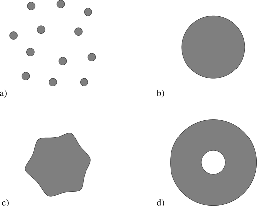
Figure 3: Configurations of noninteracting electrons in the Lowest Landau level, or planar configurations of noncommutative instantons.

A variety of configurations of electrons in the lowest Landau level are depicted in figure 3. Generic states (a) have electrons which are widely separated, and clearly correspond to states with widely separated instantons. At the opposite extreme are states for which all of the electrons come together to form a “puddle” of incompressible quantum Hall fluid. This puddle may be round (b) (corresponding to the ground state in the case that the electrons sit in a harmonic oscillator potential) or any other shape (c),(d) as long as the total area is $BN$. It is noncommutative instanton configurations corresponding to these puddle states that we would like to identify with large open membranes.

In the next subsections, we will write down explicit solutions of (52) corresponding to some of these puddle states (borrowed from Polychronakos’ studies of quantum Hall states) and show that may indeed be interpreted as open D2-branes.

8.2 The open D2-brane disk

The simplest “puddle” solution to (52) is that corresponding to the round quantum Hall droplet (figure 3b), and is given by

$$A=\sqrt{B}\left(\begin{array}[]{ccccc}0&1&&&\\ &0&\sqrt{2}&&\\ &&&\ddots&\\ &&&0&\sqrt{N-1}\\ &&&&0\end{array}\right)\qquad\qquad{\Phi}=\sqrt{B}\left(\begin{array}[]{c}0\\ 0\\ \vdots\\ 0\\ \sqrt{N}\end{array}\right)$$ (53)

This was written down by Braden and Nekrasov [29] in the context of noncommutative instantons and by Polychronakos [27] to describe the ground state of electrons in a harmonic oscillator potential in the lowest Landau level. It was argued by Berkooz in the context of the lightlike noncommutative (0,2) theory that this configuration corresponds to a round rigid open membrane.

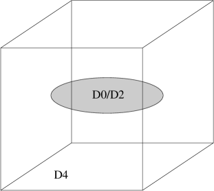
Figure 4: Noncommutative D2-brane disk in a D4-brane.

There are various ways to see that this indeed corresponds to a round open D2-brane. First, equation (51) shows that this configuration has a net D2-brane area in the $12$ plane given by $2\pi BN$, since the membrane charge (operator coupling to $C_{012}$) is ${\rm Tr}\,({\cal D}_{3})$ and the membrane tension in our units is $2\pi$. This however is true of all the noncommutative instanton configurations since each instanton carries a unit of area. To measure how this area is distributed, it is useful to determine the moments of the charge distribution. From (7.2), moments of the zero-brane charge distribution are given by derivatives of ${\cal J}^{(1)}_{0}=T^{++}$ at $k=0$. The dipole moment is

$$-i\partial_{k_{i}}{\cal J}^{(1)}_{0}(k=0)={\rm Tr}\,(X_{i})=0$$

so the charge distribution is centered at the origin. The quadrupole moments in the $x-y$ plane are

$$I_{ij}=\partial_{k_{i}}\partial_{k_{j}}{\cal J}^{(1)}_{0}(k=0)={\rm Tr}\,(X_{i}X_{j}+{1\over 2}\delta_{ij}{\Phi}{\bar{\Phi}})$$

It is straightforward to calculate

$$I_{xy}=0,\;I_{xx}=I_{yy}={1\over 2}BN^{2}$$

These are exactly the quadrupole moments of a distribution of $N$ units of charge spread uniformly over a round disk of area $2\pi BN$. Further, the moment of inertia for the D0-brane charge, $I_{xx}+I_{yy}$ is given by the trace of the operator

$$r^{2}\equiv X^{2}+Y^{2}+{\Phi}{\bar{\Phi}}=B\left(\begin{array}[]{ccccc}1&&&\\ &3&&\\ &&\ddots&\\ &&&2N-1\end{array}\right)\;.$$ (54)

The fact that this operator is diagonal with evenly spaced eigenvalues suggests that the area is evenly spaced with respect to the radius squared up to a maximum $r^{2}$ of $\sim 2BN$, as we would expect for a uniform disk. Finally, we note that in the $N=\infty$ limit, the matrix $A$ goes over to the matrix representation of a harmonic oscillator creation operator, satisfying $[A,A^{\dagger}]=B$. In terms of the real coordinates, this is $[X,Y]=iB$, which is exactly the configuration of an infinite number of D0-branes describing an infinite flat noncommutative D2-brane.

Together, these observations give good evidence that the noncommutative instanton configuration (53) may indeed be interpreted as an open noncommutative D2-brane disk of radius $R=\sqrt{2BN}$. It also provides an example of how the current operators we have derived may be used to learn about the spacetime distribution of charges for a given configuration.

8.3 Other planar open D2-branes

There are a number of transformations that permit us to generate new solutions of (52) starting from any given solution.

As pointed out in [27], given a solution of (52), the infinitesimal transformation

$$A\to A+\epsilon_{n}(A^{\dagger})^{n}$$ (55)

preserves the condition (52) and therefore generates a new solution. As explained in [27], these correspond to area-preserving deformations of the disk which change the shape of the boundary of the membrane (starting from the disk, they produce ripples with wavelength $\propto{1\over n}$). They are related to infinitesimal area preserving diffeomorphisms of the complex plane

$$z\to z+h$$

given by

$$h={\epsilon}_{n}\bar{z}^{n}$$ (56)

In fact, any function $h$ satisfying $\partial h+\bar{\partial}\bar{h}=0$ will generate an area-preserving diffeomorphism, and in general we may choose $h=\bar{\partial}(g-\bar{g})$. These are generated by (56) as well as

$$h={\epsilon}mz^{n}\bar{z}^{m-1}-\bar{{\epsilon}}n\bar{z}^{n-1}z^{m}$$ (57)

From this latter set of generators, we may guess another set of solution generating infinitesimal transformations for $A$, namely

$$A\to A+{\epsilon}_{mn}{\rm sym}(A^{n}(A^{\dagger})^{m-1})-\bar{{\epsilon}}_{mn}{\rm sym}(A^{m}(A^{\dagger})^{n-1})$$ (58)

where ${\rm sym}$ indicates a summing over all possible orderings with coefficient 1 for each independent term. It is not hard to show that these transformations preserve the constraint (52) to leading order in ${\epsilon}$.

Not all of these transformations are independent, firstly because $A^{N+1}$ may be written in terms of lower powers of $A$ and also because some of these may be equivalent to infinitesimal gauge transformations

$$A\to A+i[B+B^{\dagger},A]\qquad{\Phi}\to{\Phi}+i(B+B^{\dagger}){\Phi}\;.$$

It is straightforward to integrate some of the simpler transformations to explicitly produce new solutions. The constant $h$ transformations clearly generate translations $A\to A+z{\hbox to0.0pt{1\hss}\hskip 1.6pt\hbox{1}}$, while those linear in $z$ give $A\to\alpha A+\beta A^{\dagger}$ with $|{\alpha}|^{2}-|{\beta}|^{2}=1$, corresponding to $SL(2,R)$ transformations on the plane (rotations, shears, squashings). For example, starting from the disk and performing the $SL(2,R)$ transformation that expands the $x$ direction while contracting the $y$ direction gives the solution

$$A=\sqrt{B}\cosh(a)\left(\begin{array}[]{ccccc}0&1&&&\\ &0&\sqrt{2}&&\\ &&&\ddots&\\ &&&0&\sqrt{N-1}\\ &&&&0\end{array}\right)+\sqrt{B}\sinh(a)\left(\begin{array}[]{ccccc}0&&&&\\ 1&0&&&\\ &\sqrt{2}&0&&\\ &&&\ddots&\\ &&&\sqrt{N-1}&0\end{array}\right)$$

which should correspond to an ellipsoidal membrane with axes along the coordinate axes. As for the disk, one may calculate moments of the charge distribution, and one finds agreement with this geometrical picture.

A somewhat more complicated transformation that can be integrated readily for the case of the disk is

$$A\to A+\epsilon(A^{\dagger})^{N-1}\;.$$

As a transformation on the complex plane, this introduces $n$ ripples on the boundary of the unit disk, however, we will find a rather different interpretation for the transformation on our noncommutative open membrane disk. Solving

$$\partial_{t}A=(A^{\dagger})^{N-1}\;,$$

one finds the solution

$$A=\sqrt{B}\left(\begin{array}[]{ccccc}0&\sqrt{1+q}&&&\\ &0&\sqrt{2+q}&&\\ &&0&&\\ &&&\ddots&\sqrt{N-1+q}\\ \sqrt{q}&&&&0\end{array}\right)\qquad\qquad{\Phi}_{1}=\sqrt{B}\left(\begin{array}[]{c}0\\ 0\\ \vdots\\ 0\\ \sqrt{N}\end{array}\right)$$

where $q$ is an arbitrary parameter. This is exactly the solution written down by Polychronakos to describe a quantum Hall droplet with a quasihole of charge proportional to $q$ at the center. For a large quasi-hole, the electron fluid forms an annulus, so it seems reasonable to identify this solution with an annular open D2-brane. To verify this, note that the moment of inertia matrix for this solution is

$$r^{2}=AA^{\dagger}+A^{\dagger}A+{\Phi}{\bar{\Phi}}=B\left(\begin{array}[]{ccccc}1+q&&&&\\ &3+q&&&\\ &&\ddots&\\ &&&2N-1+q&\end{array}\right)\;.$$

As for the disk, we see that the elements of area are equally spaced in $r^{2}$, but this time from $r^{2}\sim Bq$ to $r^{2}\sim(2N+q)b$, consistent with the interpretation as a uniform annulus with inner and outer radii $\sqrt{qB}$ and $\sqrt{(2N+q)B}$ and total area $2\pi BN$, as before.

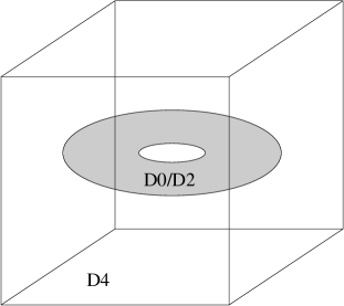
Figure 5: Annular open D2-brane configuration.

Thus, area preserving diffeomorphisms of the complex plane map to a set of transformations (55) and (58) that include both “smooth” boundary deformations of a D2-brane disk as well as transformations which create a new boundary. Using this set of transformations, it should be possibly to produce solutions corresponding to planar open membranes of arbitrary shape and topology (in the limit of large $N$). T-dualizing in directions transverse to the D4-brane, we can produce an analogous set of solutions corresponding to open D(p+2)-branes ending on D(p+4)-branes. In particular, for $p>1$, there will be a real moduli space, and these solutions will correspond to different supersymmetric vacua.

8.4 Bulging branes

We have seen in the previous section that there exist planar configurations of noncommutative instantons which have charge distributions corresponding to open D2-branes of various shapes. For these configurations, the bulk of the D2-brane sat completely inside the D4-brane, and all of the configurations were degenerate. In particular, the open D2-brane configurations could fall apart at no cost in energy to a collection of widely separated D0-branes dissolved in the D4-brane, each carrying a unit of membrane charge.

It is reasonable to ask whether such an open D2-brane configuration really behaves like a large membrane as opposed to simply a collection of individual instantons each carrying some membrane charge and arranged in the shape of a large membrane. One way to address this question would be to try and excite some collective mode of the membrane. In particular, we will attempt to pull the interior of our D2-brane disk off the D4-brane by turning on additional background fields. Since the membrane carries both D0-brane charge and D2-brane charge, we could exert a force on the membrane in a direction transverse to the D4-brane either by turning on a gradient of $C^{(1)}_{0}$ or $C^{(3)}_{012}$. We will choose to pull the membrane off by its D0-brane charge, so we turn on an additional weak background field given by

$$C^{1}_{0}=\alpha x^{9}$$

where $x^{9}$ is one of the directions perpendicular to the D4-brane. Including the new operator coupling to this background field (from (7.2)) as well as the additional terms in the potential involving the matrix $X^{9}$, the potential becomes

$$V = {\rm Tr}\,(-[A,X^{9}][A^{\dagger},X^{9}])+{\bar{\Phi}}X^{9}X^{9}{\Phi}$$ (59)

$$+{1\over 2}{\rm Tr}\,(([A,A^{\dagger}]+{\Phi}{\bar{\Phi}}-B)^{2})$$

$$+\alpha{\rm Tr}\,(X^{9})$$

We now start with the solution (53) corresponding to the D2-brane disk and look for a new solution perturbatively in ${\alpha}$. The relevant equations of motion are

$$0 = [A,[A^{\dagger},X^{9}]]+[A^{\dagger},[A,X^{9}]]+{\Phi}{\bar{\Phi}}X^{9}+X^{9}{\Phi}{\bar{\Phi}}+{\alpha}$$

$$0 = [[A,X^{9}],X^{9}]+[[A,A^{\dagger}]+{\Phi}{\bar{\Phi}},A]$$

$$0 = X^{9}X^{9}{\Phi}+([A,A^{\dagger}]+{\Phi}{\bar{\Phi}}-B){\Phi}$$

We expect that the final configuration should retain the rotational symmetry in the 1-2 plane, so that each value of $r^{2}$ (where $r$ is the distance from the centre of the D2-brane) should correspond to a particular value of $X^{9}$. Since the $r^{2}$ matrix (54) of the unperturbed solution was diagonal, we therefore look for a solution for which $X^{9}$ is also diagonal. It is not hard to show that to leading order in ${\alpha}$, the equations of motion are solved by

$$A=A_{0}+{\cal O}({\alpha}^{2})\;,\;\;{\Phi}={\Phi}_{0}+{\cal O}({\alpha}^{2})\;,\;\;X^{9}=-{\alpha\over 2B}\left(\begin{array}[]{ccccc}N&&&\\ &N-1&&\\ &&\ddots&\\ &&&1\end{array}\right)+{\cal O}({\alpha}^{2})$$

where $A_{0}$ and ${\Phi}_{0}$ are the unperturbed disk solution given in (53). Recalling that the $r^{2}$ matrix was

$$r^{2}=B\left(\begin{array}[]{ccccc}1&&&\\ &3&&\\ &&\ddots&\\ &&&2N-1\end{array}\right)$$

we see that

$$X^{9}=-{{\alpha}\over 4B^{2}}(B(2N+1)-r^{2})$$

is satisfied exactly as a matrix equation. This suggests that the perturbed membrane solution has a well defined parabolic $x^{9}(r)$ profile given by

$$x^{9}\sim-{{\alpha}\over 4B^{2}}(R^{2}-r^{2})\;,$$

as depicted in figure 6. Thus, only the boundary of the D2-brane remains attached to the D4-brane.

Substituting our solution back into the potential (59), we find that to order ${\alpha}^{2}$, the energy of the perturbed solution is

$$E=-{{\alpha}^{2}\over 8B^{2}}N(N+1)\approx-{{\alpha}^{2}\over 32B^{4}}R^{4}=-{{\alpha}^{2}\over 32\pi^{2}B^{4}}{\rm Area}^{2}$$

Since this energy scales like the square of area, it is clear that two widely separated D2-brane disks will prefer to come together to form a single bulging D2-brane rather than two separate ones. Similarly, we expect that upon turning on this background field, a general planar collection of noncommutative instantons will prefer to merge into a single open-D2 brane which allows for the maximal bulge off the D4-brane. It would be interesting to verify this more explicitly.

Figure 6: Bulging noncommutative open D2-brane.

We should note that just as for the constant $F_{0ijk}$ in Myers’ spherical D2-brane example, the constant $\partial_{9}C^{(0)}$ field we have considered is not by itself a consistent background of string theory since it carries energy density and will induce a non-zero curvature. However, for weak fields, the effects from this curvature will be at higher order in the small parameter ${\alpha}$, so we do not expect the resulting configuration for a consistent string theory background to be qualitatively different.

9 Higher order terms

In section 6, we derived leading terms in the currents of the Berkooz-Douglas matrix model starting with a rather incomplete expression for $T^{++}$. We found that the leading terms in this expression involving the fundamental fields were actually fixed by demanding consistency with the supersymmetry relations (13), various conservation relations, and symmetries. It is possible that higher order terms in $T^{++}$ might be determined in a similar way from these terms. Rather than following this approach and attempting to derive these higher order terms, in this section we use a different approach to suggest a more complete expression for $T^{++}$. If correct, this could be used as a starting point to derive complete expressions for the remaining currents in the Berkooz-Douglas model.

We begin by considering $N$ D0-branes in the presence of $k$ coincident D4-branes in the weak coupling, $\alpha^{\prime}\to 0$ limit of type IIA string theory. In this context, our desired current $T^{++}$ is the operator which measures the density of D0-brane charge. Specifically, we would like to consider supersymmetric configurations on the (classical) Higgs branch of theory where all the D0-branes are dissolved in the D4-brane. These configurations have two alternate descriptions in string theory.

In the first picture, we describe the configuration explicitly in terms of the 0-0 and 0-4 string degrees of freedom. Supersymmetric configurations are those for which the potential in the D0-brane quantum mechanics vanishes,

$$\sigma^{A}_{\rho}{}^{\sigma}({1\over 2}[{\bar{X}}^{{\rho}{\dot{\rho}}},X_{{\sigma}{\dot{\rho}}}]-{\Phi}_{\sigma}{\bar{\Phi}}^{\rho})=0\;.$$ (60)

Note that we are assuming $X^{a}$ is zero since we are on the Higgs branch. For these solutions, it is consistent to set the D4-brane fields arising from 4-4 stings to zero.

In the second picture, we describe everything in terms of the gauge field on the D4-brane. Here, supersymmetric configurations are $N$-instanton solutions to the Yang-Mills equations. In this description, we simply do not include the 0-0 string or 0-4 string degrees of freedom, since these are already described by the parameters describing the locations and sizes of the instantons. For this description to be valid, the scale size of the instantons should be much larger than the string scale.

The situation is similar to a set of D3-branes in string theory which may be described either by including the D3-brane worldvolume degrees of freedom explicitly and choosing a flat background for the closed strings or by thinking completely in terms of closed strings moving on the D3-brane geometry.

For the D0-D4 case, there is an explicit map between the two descriptions given by the ADHM construction. This construction takes fields $X_{{\rho}{\dot{\rho}}}$ and ${\Phi}_{\rho}$ satisfying the ADHM equations (60) and computes a gauge field $A_{i}(X_{{\rho}{\dot{\rho}}},{\Phi}_{\rho};x^{i})$ which is a self-dual solution to the Yang-Mills equations in the $N$ instanton sector. This construction will be very useful for our purposes, since in the pure D4-brane language, the operator measuring D0-brane charge is well known,

$${\rho}(x)={\rm Tr}\,(F\wedge F)\;.$$ (61)

Since the D0-brane charge density should be the same regardless of what description we use, it must be that the D0-brane density in the first picture is given by (61) where $F$ is taken to be the field strength computed from the gauge field determined by the ADHM construction from $X_{{\rho}{\dot{\rho}}}$ and ${\Phi}_{\rho}$.

We will now be more explicit. Let the spatial coordinates of the D4-brane be denoted $x^{i}$, or in the $SU(2)\times SU(2)$ notation, $x_{{\rho}{\dot{\rho}}}$. Then given fields $X_{{\rho}{\dot{\rho}}}$ and ${\Phi}_{\rho}$ satisfying (60) and defining $Z_{{\rho}{\dot{\rho}}}=X_{{\rho}{\dot{\rho}}}-x_{{\rho}{\dot{\rho}}}$, the ADHM gauge field is given by

$$A_{i}=\Lambda^{\dagger}\partial_{i}\Lambda+\psi_{\dot{\rho}}^{\dagger}\partial_{i}\psi^{\dot{\rho}}$$

where $\Lambda$ and $\psi_{\dot{\rho}}$ are each $k\times k$ matrices satisfying

$$Z_{{\rho}{\dot{\rho}}}\psi^{\dot{\rho}}={\Phi}_{\rho}\Lambda$$ (62)

and normalized such that

$$\Lambda^{\dagger}\Lambda+\psi_{\dot{\rho}}^{\dagger}\psi^{\dot{\rho}}={\hbox to0.0pt{1\hss}\hskip 1.6pt\hbox{1}}$$

For generic configurations, we may use these formulae to calculate the density ${\rm Tr}\,(F\wedge F)$ directly in terms of $X$ and ${\Phi}$. Defining

$$f=2(Z_{{\rho}{\dot{\rho}}}\bar{Z}^{{\rho}{\dot{\rho}}}+{\Phi}_{\rho}{\bar{\Phi}}^{\rho})^{-1}$$

and

$$B_{\rho}^{\sigma}={1\over 2\pi}f(\delta^{\sigma}_{\rho}-\bar{Z}^{{\sigma}{\dot{\rho}}}fZ_{{\rho}{\dot{\rho}}})$$

we find (for more details, see for example [30])

$${\rho}(x) = {\rm Tr}\,(F\wedge F)$$

$$= {\rm Tr}\,((B_{\rho}^{\sigma}\sigma^{B}_{\sigma}{}^{\alpha})^{2})$$

$$= {\rm Tr}\,(2B_{\rho}^{\rho}B_{\sigma}^{\sigma}-B_{\rho}^{\sigma}B_{\sigma}^{\rho})$$

This is the position space D0-brane charge distribution for a general configuration on the instanton moduli space. Since the ADHM mapping assumes that the ADHM equations are satisfied, the operator $\rho(x)$ can only be expected to agree with our desired operator $T^{++}$ up to terms that vanish when the equations of motion are satisfied. Thus, we may conclude that

$$T^{++}(k^{a}=X^{a}=0,{\rm on\;shell})={\rho}(x)$$

To make a comparison with our previous expression for $T^{++}$, we should go to momentum space, however it seems rather tricky to Fourier transform the general expression ${\rho}(x)$. Things simplify considerably if we consider the special case of a single D0-brane. Here, the expression for ${\rho}$ becomes simply

$${\rho}(x)={6\over\pi^{2}}{({\Phi}_{\rho}{\bar{\Phi}}^{\rho})^{2}\over({\Phi}_{\rho}{\bar{\Phi}}^{\rho}+|x-X|^{2})^{4}}$$ (64)

After rewriting the denominator using

$${1\over t^{4}}={1\over 6}\int_{0}^{\infty}d{\alpha}{\alpha}^{3}e^{-{\alpha}t}$$

it is straightforward to transform to momentum space, and we find

$${\rho}(k)=e^{ik\cdot X}\int_{0}^{\infty}d{\alpha}{\alpha}e^{-{\alpha}-{1\over 4{\alpha}}k^{2}{\Phi}_{\rho}{\bar{\Phi}}^{\rho}}$$ (65)

Expanding in powers of momentum, we find

$${\rho}(k)=e^{ik\cdot X}(1-{1\over 4}\bar{k}^{{\rho}{\dot{\rho}}}k_{{\rho}{\dot{\rho}}}{\Phi}_{\rho}{\bar{\Phi}}^{\rho}+{\cal O}(k^{4}))$$

which precisely agrees with our previous expression for ${\cal J}_{(1)}^{0}=T^{++}$. This gives evidence that (65) may indeed provide a complete expression for $T^{++}$ for the case of a single D0-brane, up to terms that vanish when the ADHM equations

$${\Phi}_{\rho}{\bar{\Phi}}^{\sigma}={1\over 2}\delta_{\rho}^{\sigma}{\Phi}_{\alpha}{\bar{\Phi}}^{\alpha}\;.$$

are satisfied. The simplest possibility would be that these extra terms are zero and that (65) is the correct operator off-shell. To test this, one could use the methods of section 6 and check whether this expression is a consistent starting point for the supersymmetry relations.

To summarize, we have argued that a complete expression for the zero-brane density operator ${\cal J}_{(1)}^{0}=T^{++}$ in the ${\alpha}^{\prime}\to 0$ limit may be given in position space by (9) and in momentum space for the case of a single D0-brane by (65), up to terms which vanish when the ADHM equations are satisfied. Assuming the validity of these expressions, one could use the methods of section 6 to obtain more complete expressions for the remaining currents.

9.1 A puzzle

Up to order $k^{2}$, we found that the expression ${\rho}(k)$ in (65) agrees with our previous expression for $T^{++}$. However, note that if one tries to expand the expression (65) further, one finds that the $k^{4}$ term is infinite (the ${\alpha}$ integral diverges once we bring down two powers of ${1\over{\alpha}}$). Thus, while the expression (65) is clearly well defined for all values of ${\Phi}$ and $k$ (the integral is always finite), it is not analytic at $k=0$. The leading singularity is of the form $k^{4}\log(k^{2})$.

In fact, this behavior should have been expected. Recall that various terms in the momentum expansion of the current $T^{++}$ correspond to multipole moments of the zero-brane charge distribution. However from (64), it is clear that the charge distribution for an instanton configuration falls off only algebraically, as ${1\over r^{8}}$ in the D4-brane directions. Thus, integrating this distribution over the D4-brane worldvolume with more than three powers of $x^{i}$ will give a divergent result. In other words, multipole moments beyond the octopole moment cannot be defined since the charge distribution does not fall off fast enough. Thus the non-analyticity of $T^{++}$ at $k=0$ is consistent with physical expectations. This is not the puzzle.

The puzzle comes when we consider the string theory effective action, which includes the term

$$\int dtd^{9}k\;C^{(1)}_{0}(-k,t)T^{++}(k,t)\;.$$ (66)

Typically, one expects to be able to calculate terms in the classical string theory effective action by computing tree-level amplitudes with specific numbers of vertex operators. For example, the $C^{(1)}{\Phi}{\bar{\Phi}}$ term should come from a disk amplitude with one Ramond-Ramond closed string vertex operator inserted on the bulk of the worldsheet and two $0-4$ open string vertex operators inserted on the boundary. On the other hand, the terms in (66) with four 0-4 fields are (by dimensional analysis) also the terms at order $k^{4}$ in a momentum expansion, and we have argued that such terms are not well defined on their own (since the 16-pole moment is not well-defined). This suggests that in computing the five-point function with one RR vertex operator and four 0-4 string vertex operators, one would encounter a divergence that could be cured only by summing over the complete set of disk amplitudes with arbitrary numbers of 0-4 vertex operators. To reiterate, if the $C^{(1)}k^{4}{\Phi}^{4}$ term by itself were finite, it would indicate that instanton configurations should have well defined 16-pole moments, inconsistent with the ${1\over r^{8}}$ falloff.

One way around this conclusion could be that the charge density operator takes the singular form (65) only after integrating out some light field. A natural candidate might be the 4-4 string fields, but these can be included explicitly in the effective action and give the usual $C_{0}Tr(F\wedge F)$ term. In the description of instantons in terms of the 0-0 and 0-4 string degrees of freedom, the D4-brane gauge field can be consistently set to zero, so this additional term does not contribute to the charge density. Thus, it is not clear to us what the extra light field could be.

If it is true that the five point function has a divergence, we would have the interesting situation of apparently having to sum over an infinite set of string amplitudes to obtain the effective action. This is reminiscent of dealing with infrared divergences in field theory. Before speculating further, it seems worthwhile to directly study the five point function in question to check whether there is actually a divergence. We leave this as a problem for future work.

10 Remarks

In this paper, we have derived leading terms in the operators which describe supergravity currents in the Berkooz-Douglas matrix model of M-theory with M5-branes. We used these operators to write down leading terms in the action describing linear couplings of type II supergravity fields to systems with arbitrary numbers of Dp-branes and D(p+4)-branes in string theory. Using these explicit actions, we demonstrated situations in which turning on certain background fields allows a collection of D0-branes to form a stable open D2-brane ending on a D4 brane, including planar configurations in which the D2-brane sits completely inside the D4-brane, as well as a bulging brane configuration with the D2-brane attached only at the boundary. The current operators we derived provide a valuable tool to determine the spacetime configuration of charges for a given matrix configuration and thus to provide a geometrical picture for the configurations we have studied.

There are numerous directions for future work. Firstly, it would be interesting to determine more complete expressions for the currents. We have explicitly calculated leading terms in a momentum expansion (corresponding to low order moments) of the currents starting with the leading terms in the primary current $T^{++}$ (corresponding to the zero-brane density). A more complete expression (up to equation of motion terms) for $T^{++}$ was proposed in section 9, based on the ADHM construction, and this could serve as a starting point for deriving full expressions for the other currents, though the expression we have given is only required to be valid on-shell. It is possible that some of the ambiguous terms (possible extra terms which vanish when the ADHM equations are satisfied) might be fixed by consistency with the supersymmetry relations. If the expression we have proposed is correct, it would also be interesting to understand how it could arise from string theory amplitudes, since it does not have a well defined expansion in momenta or in the number of open string fields.

It would also be interesting to find and study other noncommutative open brane configurations using the actions we have derived. For example, there should be situations (e.g. ones related to those we have studied by boosting) for which the open D2-brane is stabilized by a combination of background fields and motion within the D4-brane (analogous to the closed brane configurations studied in [31]). Other interesting configurations might arise in situations with more than one D4-brane, perhaps separated in some transverse direction. More generally, it would be nice to have a description of arbitrarily shaped open D2-branes for various topologies (such as the one for closed membranes of spherical [2] and toroidal [5] topology). The solution-generating set of transformations given in section 8.3 would probably be quite useful in this regard.

We have seen that the actions for various Dp-D(p+4) systems are related by T-duality in the directions transverse to both sets of branes or shared by both sets of branes. One could also perform T-duality in the other directions to derive actions for perpendicular brane systems. For example, starting with the D0-D4 system and T-dualizing in two of the D4-brane directions, we arrive at a system with two perpendicular sets of D2-branes. Couplings of supergravity fields to the worldvolume fields in this system would follow immediately from the results of this paper.

Another application would be to the study of 3+1 dimensional field theories living on D3-branes in the presence of D7-branes. These are ${\cal N}=2$ supersymmetric gauge theories in the absence of background fields, but can be deformed to theories with less supersymmetry by turning on various operators. Our results give all relevant and marginal operators that can be turned on in the presence of any constant supergravity potential or field strength.

A rather different application of this work might be to the search for an off-shell formulation of eleven-dimensional supergravity. In deriving the supersymmetry relations between Matrix theory currents, we needed to include “auxiliary” terms to account for the fact that the supersymmetry variation of the action is only required to vanish on shell, that is when the equations of motion for the bulk supergravity fields are satisfied. If an off shell formulation of D=11 supergravity exists, one should be able to write down a set of currents coupling to all the fields including the auxiliary fields. This expanded set of currents would then be required to obey a set of supersymmetry relations without any auxiliary terms. By examining the structure of the auxiliary terms we have derived (e.g. in the BFSS Matrix model) and interpreting these as a set of auxiliary currents, one might be able to deduce some of the auxiliary fields that would be required in an off-shell formulation of eleven-dimensional supergravity (if such a formulation exists). A similar approach was employed in [32] to deduce the existence of certain auxiliary fields in d=10 N = 1 supergrvaity based on the supersymmetry transformation properties of currents in d=10, ${\cal N}=1$ Yang-Mills theory to which the supegravity theory can couple. A recent discussion of some progress towards an off-shell formulation of eleven-dimensional supergravity may be found in [33].

Finally, it would be interesting to compare our description of noncommutative open D2-branes in terms of D0-brane degrees of freedom with an alternate description directly in terms of D2-brane degrees of freedom (with a B field on the D2-brane worldvolume). The relationship between these two descriptions would be something like a Seiberg-Witten map ([34]) for field theories on noncommutative spaces with boundaries.

Appendix A ${\cal N}=1$ in six dimensions

The actions for $Dp-D(p+4)$ systems and for the Matrix model of M-theory with M5-branes considered in this paper are written using the language of $D=6$ supersymmetric field theory with eight supercharges (${\cal N}=2$ supersymmetry when reduced to four dimensions). The allowed non-gravitational multiplets are vector multiplets, hypermultiplets and tensor multiplets, however only the first two arise in the $Dp-D(p+4)$ actions we consider. The most general action for an arbitrary number of vector and hypermultiplets that is renormalizable when reduced to four dimensions may be written as

$${\cal L} = {\rm Tr}\left(-{1\over 4}F_{\mu\nu}F^{\mu\nu}-{i\over 2}\bar{\lambda}^{\rho}\gamma^{\mu}D_{\mu}\lambda_{\rho}\right)$$

$$-D_{\mu}\bar{\Phi}^{\rho}D^{\mu}\Phi_{\rho}-{i\over 2}\bar{\chi}\gamma^{\mu}D_{\mu}\chi$$

$$+i\epsilon^{\alpha\beta}\bar{\chi}\lambda_{\alpha}\Phi_{\beta}-i\epsilon_{\alpha\beta}\bar{\Phi}^{\alpha}\bar{\lambda}^{\beta}\chi$$

$$-{1\over 2}\left(2\bar{\Phi}^{\alpha}{\rm t}^{a}\Phi_{\beta}\bar{\Phi}^{\beta}{\rm t}^{a}\Phi_{\alpha}-\bar{\Phi}^{\alpha}{\rm t}^{a}\Phi_{\alpha}\bar{\Phi}^{\beta}{\rm t}^{a}\Phi_{\beta}\right)$$

We use conventions such that $F_{\mu\nu}=\partial_{\mu}A_{\nu}-\partial_{\nu}A_{\mu}+i[A_{\mu}A_{\nu}]$ and $D_{\mu}=\partial_{\mu}+iA^{a}_{\mu}t^{a}$.

The action is invariant under the following supersymmetry transformations,

$$\delta A_{\mu}^{a} = -i\bar{\zeta}^{\rho}\gamma_{\mu}\lambda^{a}_{\rho}$$

$$\delta\lambda^{a}_{\rho} = {1\over 2}F^{a}_{\mu\nu}\gamma^{\mu\nu}\zeta_{\rho}+2i\zeta_{\alpha}\bar{\Phi}^{\alpha}{\rm t}^{a}\Phi_{\rho}-i\zeta_{\rho}\bar{\Phi}^{\alpha}{\rm t}^{a}\Phi_{\alpha}$$

$$\delta\Phi^{i}_{\alpha} = \epsilon_{\alpha\beta}\bar{\zeta}^{\beta}\chi^{i}$$

$$\delta\chi^{i} = 2i\epsilon^{\alpha\beta}D_{\mu}\Phi^{i}_{\alpha}\gamma^{\mu}\zeta_{\beta}$$

Appendix B Useful manipulations in six dimensions

In this paper, we frequently convert ten-dimensional expressions covariant under $SO(9,1)$ Lorentz symmetry into six dimensional expressions for which the manifest symmetry group is $SO(5,1)\times SO(4)\sim SO(5,1)\times SU(2)_{R}\times SU(2)_{L}$. To convert bosonic expressions, the only non-trivial step is to write various $SO(4)$ representations in terms of the $SU(2)\times SU(2)$ notation.

Firstly, in $SU(2)\times SU(2)$ language, a vector $X^{i}$ of $SO(4)$ becomes

$$X_{{\rho}{\dot{\rho}}}={1\over\sqrt{2}}\left(\begin{array}[]{cc}X^{6}+iX^{7}&-X^{8}+iX^{9}\\ X^{8}+iX^{9}&X^{6}-iX^{7}\end{array}\right)$$ (67)

transforming in the $(2,2)$ representation of $SU(2)\times SU(2)$ with the reality condition

$$X_{{\rho}{\dot{\rho}}}={\epsilon}_{{\rho}{\sigma}}{\epsilon}_{{\dot{\rho}}{\dot{\sigma}}}X^{{\sigma}{\dot{\sigma}}}\;.$$

The normalization is chosen so that

$$X^{i}X^{i}={\bar{X}}^{{\rho}{\dot{\rho}}}X_{{\rho}{\dot{\rho}}}$$

An antisymmetric tensor $A_{ij}$ of $SO(4)$ splits into self-dual and anti-self-dual parts transforming in the ${\bf 3}$ of $SU(2)_{L}$ and $SU(2)_{R}$ respectively. Defining

$$A^{\rho}{}_{\sigma}=A^{{\rho}{\dot{\rho}}}{}_{{\sigma}{\dot{\rho}}}\;\qquad A^{\dot{\rho}}{}_{\dot{\sigma}}=A^{{\rho}{\dot{\rho}}}{}_{{\rho}{\dot{\sigma}}}\;.$$

we have

$$A^{{\rho}{\dot{\rho}}}{}_{{\sigma}{\dot{\sigma}}}={1\over 2}\delta^{\rho}_{\sigma}A^{\dot{\rho}}{}_{\dot{\sigma}}+{1\over 2}\delta^{\dot{\rho}}_{\dot{\sigma}}A^{\rho}{}_{\sigma}$$

Alternately, we can describe these tensors as real $SO(3)$ vectors

$$A_{A}={i\sqrt{2}\over 4}A^{{\rho}{\dot{\rho}}}{}_{{\sigma}{\dot{\rho}}}{\sigma}^{A}_{\rho}{}^{\sigma}\;\qquad A_{\dot{A}}={i\sqrt{2}\over 4}A^{{\rho}{\dot{\rho}}}{}_{{\rho}{\dot{\sigma}}}{\sigma}^{\dot{A}}_{\dot{\rho}}{}^{\dot{\sigma}}$$

where $A$ and $\dot{A}$ are fundamental $SO(3)_{R}$ and $SO(3)_{L}$ indices. With these normalizations

$${1\over 2}A_{ij}B_{ij}=A_{A}B_{A}+A_{\dot{A}}B_{\dot{A}}$$

From a three-index antisymmetric tensor $A_{ijk}$ we define

$$A_{{\rho}{\dot{\rho}}}\equiv{1\over 3}{\epsilon}^{{\alpha}{\beta}}{\epsilon}^{{\dot{\alpha}}{\dot{\beta}}}A_{{\rho}{\dot{\alpha}}\;{\alpha}{\dot{\beta}}\;{\beta}{\dot{\rho}}}$$

Finally, we will write a four-index antisymmetric tensor $A_{ijkl}$ as

$$A\equiv{1\over 24}{\epsilon}^{ijkl}A_{ijkl}=-{1\over 12}A^{{\rho}{\dot{\rho}}}{}_{{\rho}{\dot{\sigma}}}{}^{{\sigma}{\dot{\sigma}}}{}_{{\sigma}{\dot{\rho}}}$$

To write ten-dimensional expressions involving fermions in six dimensional notation we note that a sixteen component Majorana-Weyl spinor in the ${\bf 16}$ of $SO(9,1)$ splits into a pair of spinors in the ${\bf(4,2,1)}$ and ${\bf(4,1,2)}$ of $SO(5,1)\times SU(2)\times SU(2)$. Fermion bilinears may be reduced using

$${\bar{\lambda}}\gamma^{\mu}\chi = {\bar{\lambda}}^{\rho}\gamma^{\mu}{\chi}_{\rho}+{\bar{\lambda}}^{{\dot{\rho}}}\gamma^{\mu}{\chi}_{\dot{\rho}}$$

$${\bar{\lambda}}\gamma^{\mu\nu\lambda}\chi = {\bar{\lambda}}^{\rho}\gamma^{\mu\nu\lambda}{\chi}_{\rho}+{\bar{\lambda}}^{{\dot{\rho}}}\gamma^{\mu}{\chi}_{\dot{\rho}}$$

$$A_{i}{\bar{\lambda}}\gamma^{i}\chi = -\sqrt{2}i\bar{A}^{{\rho}{\dot{\rho}}}\{{\epsilon}_{{\sigma}{\rho}}{\bar{\lambda}}^{\sigma}\chi_{\dot{\rho}}+{\epsilon}^{{\dot{\rho}}{\dot{\sigma}}}{\lambda}^{\dot{\sigma}}{\chi}_{r}\}$$

$$A_{\mu\nu i}{\bar{\lambda}}\gamma^{\mu\nu i}\chi = -\sqrt{2}i\bar{A}_{\mu\nu}{}^{{\rho}{\dot{\rho}}}\{{\epsilon}_{{\sigma}{\rho}}{\bar{\lambda}}^{\sigma}\gamma^{\mu\nu}\chi_{\dot{\rho}}+{\epsilon}^{{\dot{\rho}}{\dot{\sigma}}}{\lambda}^{\dot{\sigma}}\gamma^{\mu\nu}{\chi}_{r}\}$$

$${1\over 2}A_{\mu ij}{\bar{\lambda}}\gamma^{\mu ij}\chi = \sqrt{2}i\{A_{\mu A}{\bar{\lambda}}^{\rho}\sigma^{A}_{\rho}{}^{\sigma}\gamma^{\mu}\chi_{\sigma}+A_{\mu\dot{A}}{\bar{\lambda}}^{\dot{\rho}}\sigma^{\dot{A}}_{\dot{\rho}}{}^{\dot{\sigma}}\gamma^{\mu}\chi_{\dot{\sigma}}\}$$

Additional formulae useful in manipulating expressions in our notation are

$${\bar{\lambda}}\gamma_{\mu_{1}\cdots\mu_{n}}\chi=(-1)^{n}{\bar{\chi}}^{c}\gamma_{\mu_{n}\cdots\mu_{1}}\lambda^{c}$$

$$A_{[{\rho}}B_{{\sigma}}C_{\tau]}=0$$

$${\epsilon}_{{\rho}{\sigma}}A_{\tau}+{\epsilon}_{{\sigma}\tau}A_{\rho}+{\epsilon}_{\tau{\rho}}A_{\sigma}=0$$

$$\sigma^{A}_{\rho}{}^{\sigma}\sigma^{A}_{\alpha}{}^{\beta}=2\delta_{\rho}^{\beta}\delta_{\sigma}^{\alpha}-\delta_{\rho}^{\sigma}\delta_{\alpha}{}^{\beta}$$

Finally, in manipulating expressions with three or more spinors, it is often necessary to use Fierz identities which may be derived from the completeness relation

$$M_{{\alpha}{\beta}} = {1\over 4}{\rm Tr}\,(M\gamma_{0})(\gamma^{0})_{{\alpha}{\beta}}+{1\over 4}{\rm Tr}\,(M\gamma_{\mu}\gamma_{0})(\gamma^{0}\gamma^{\mu})_{{\alpha}{\beta}}+{1\over 8}{\rm Tr}\,(M\gamma_{\nu\mu}\gamma_{0})(\gamma^{0}\gamma^{\mu\nu})_{{\alpha}{\beta}}$$

$$+{1\over 48}{\rm Tr}\,(M\gamma_{\lambda\nu\mu}\gamma_{0})(\gamma^{0}\gamma^{\mu\nu{\lambda}})_{{\alpha}{\beta}}$$

For spinors $\lambda$ and $\theta$ of opposite chirality, we find

$$\theta{\bar{\lambda}} = -{1\over 4}({\bar{\lambda}}{\theta}){\hbox to0.0pt{1\hss}\hskip 1.6pt\hbox{1}}-{1\over 4}({\bar{\lambda}}\gamma^{0a}{\theta})\gamma^{0a}+{1\over 8}({\bar{\lambda}}\gamma^{ab}{\theta})\gamma^{ab}\;.$$

For spinors $\theta$ and $\chi$ of the same chirality, we have

$${\theta}{\bar{\chi}}={1\over 4}({\bar{\chi}}\gamma^{0}{\theta})\gamma^{0}-{1\over 4}({\bar{\chi}}\gamma^{a}{\theta})\gamma^{a}-{1\over 8}({\bar{\chi}}\gamma^{0ab}{\theta})\gamma^{0ab}\;.$$

Appendix C Conserved currents in the Berkooz-Douglas model

The eleven-dimensional supersymmetry algebra is given by

$$\{Q_{\alpha},Q_{\beta}\}=2P_{\mu}(\Gamma^{\mu}\Gamma^{0})_{{\alpha}{\beta}}+c_{2}Z_{\mu\nu}(\Gamma^{\mu\nu}\Gamma^{0})_{{\alpha}{\beta}}+c_{5}Z_{\mu_{1}\cdots\mu_{5}}(\Gamma^{\mu_{1}\cdots\mu_{5}}\Gamma^{0})_{{\alpha}{\beta}}$$ (68)

Here $Z_{\mu\nu}$ and $Z_{\mu_{1}\cdots\mu_{5}}$ are central charges corresponding to the membrane and five-brane respectively. In the presence of a five-brane oriented along the $0,1,2,3,4,5$ directions, the preserved supersymmetries are those given by ${\cal P}_{+}Q^{+}\equiv{1\over 2}(1+\Gamma)Q=Q$, where $\Gamma=\Gamma^{012345}$.

From (68), the commutator of the preserved supersymmetries becomes

$$\{Q^{+}_{\alpha},Q^{+}_{\beta}\} = 2P_{a}({\cal P}_{+}\Gamma^{a}\Gamma^{0})_{{\alpha}{\beta}}$$

$$+2c_{2}Z_{ia}({\cal P}_{+}\Gamma^{ia}\Gamma^{0})_{{\alpha}{\beta}}$$

$$+5c_{5}Z_{ijkla}({\cal P}_{+}\Gamma^{ijkla}\Gamma^{0})_{{\alpha}{\beta}}$$

$$+10c_{5}Z_{ijabc}({\cal P}_{+}\Gamma^{ijabc}\Gamma^{0})_{{\alpha}{\beta}}$$

$$+c_{5}Z_{abcde}({\cal P}_{+}\Gamma^{abcde}\Gamma^{0})_{{\alpha}{\beta}}$$

The central charges appearing on the right hand side are the momentum in the 5-brane directions, the charge of a membrane sharing one direction with the 5-brane, and the charge of a 5-brane sharing 1, 3, or 5 directions with the brane. These central charges will commute with the Hamiltonian and therefore correspond to the conserved currents of the theory. In terms of the momentum space currents of the Berkooz-Douglas model, we therefore expect the following conservation laws (for further discussion, see [24])

$$\dot{T}^{++} = ik_{a}T^{+a}+\bar{k}^{{\rho}{\dot{\rho}}}T^{+}{}_{{\rho}{\dot{\rho}}}$$

$$\dot{S}^{+}_{+{\dot{\rho}}} = ik_{a}(S_{+}^{a})_{\dot{\rho}}+i\bar{k}^{s{\dot{\sigma}}}(S_{+{\sigma}{\dot{\sigma}}})_{\dot{\rho}}$$

$$\dot{T}^{+}{}_{{\rho}{\dot{\rho}}} = ik_{a}T^{a}{}_{{\rho}{\dot{\rho}}}+i\bar{k}^{{\sigma}{\dot{\sigma}}}T_{{\sigma}{\dot{\sigma}}\;{\rho}{\dot{\rho}}}$$

$$\dot{J}^{+a}{}_{{\rho}{\dot{\rho}}} = ik_{b}J^{ba}{}_{{\rho}{\dot{\rho}}}-{\sqrt{2}\over 2}k_{{\sigma}{\dot{\rho}}}{\sigma}^{A}_{\rho}{}^{\sigma}J^{aA}-{\sqrt{2}\over 2}k_{{\rho}{\dot{\sigma}}}{\sigma}^{\dot{A}}_{\dot{\rho}}{}^{\dot{\sigma}}J^{a\dot{A}}$$

$$\dot{S}_{-{\rho}}^{+} = ik_{a}(S_{-}^{a})_{\rho}+i\bar{k}^{s{\dot{\sigma}}}(S_{-{\sigma}{\dot{\sigma}}})_{\rho}$$

$$\dot{T}^{+-} = ik_{a}T^{a-}+i\bar{k}^{{\sigma}{\dot{\sigma}}}T^{-}{}_{{\sigma}{\dot{\sigma}}}$$

$$\dot{J}^{+-a} = ik_{b}J^{b-a}+i\bar{k}^{{\sigma}{\dot{\sigma}}}J^{-a}{}_{{\sigma}{\dot{\sigma}}}$$

$$\dot{M}^{+-bcde} = ik_{a}M^{a-bcde}+i\bar{k}^{{\sigma}{\dot{\sigma}}}M_{{\sigma}{\dot{\sigma}}}{}^{-bcde}$$

$$\dot{M}^{+-A} = ik_{a}M^{a-A}+i\bar{k}^{{\sigma}{\dot{\sigma}}}M_{{\sigma}{\dot{\sigma}}}{}^{-A}$$

$$\dot{M}^{+-\dot{A}} = ik_{a}M^{a-\dot{A}}+i\bar{k}^{{\sigma}{\dot{\sigma}}}M_{{\sigma}{\dot{\sigma}}}{}^{-\dot{A}}$$

$$\dot{M}^{+-} = ik_{a}M^{a-}+i\bar{k}^{{\sigma}{\dot{\sigma}}}M_{{\sigma}{\dot{\sigma}}}{}^{-}$$

References

• [1] E. Witten, “Bound States Of Strings And p-Branes,” Nucl. Phys. B 460, 335 (1996) [arXiv:hep-th/9510135].
• [2] D. Kabat and W. Taylor, “Spherical membranes in matrix theory,” Adv. Theor. Math. Phys.  2, 181 (1998) [arXiv:hep-th/9711078].
• [3] S. J. Rey, “Gravitating M(atrix) Q-balls,” arXiv:hep-th/9711081.
• [4] T. Banks, N. Seiberg and S. H. Shenker, “Branes from matrices,” Nucl. Phys. B 490, 91 (1997) [arXiv:hep-th/9612157].
• [5] T. Banks, W. Fischler, S. H. Shenker and L. Susskind, “M theory as a matrix model: A conjecture,” Phys. Rev. D 55, 5112 (1997) [arXiv:hep-th/9610043].
• [6] W. Taylor and M. Van Raamsdonk, “Multiple D0-branes in weakly curved backgrounds,” Nucl. Phys. B 558, 63 (1999) [arXiv:hep-th/9904095].
• [7] W. Taylor and M. Van Raamsdonk, “Multiple Dp-branes in weak background fields,” Nucl. Phys. B 573, 703 (2000) [arXiv:hep-th/9910052].
• [8] R. C. Myers, “Dielectric-branes,” JHEP 9912, 022 (1999) [arXiv:hep-th/9910053].
• [9] A. Strominger, “Open p-branes,” Phys. Lett. B 383, 44 (1996) [arXiv:hep-th/9512059]. 9512059;
• [10] M. Berkooz and M. R. Douglas, “Five-branes in M(atrix) theory,” Phys. Lett. B 395, 196 (1997) [arXiv:hep-th/9610236].
• [11] M. Li, “Open membranes in matrix theory,” Phys. Lett. B 397, 37 (1997) [arXiv:hep-th/9612144]. 9612144;
• [12] M. Berkooz, “Light-like (2,0) noncommutativity and light-cone rigid open membrane theory,” arXiv:hep-th/0010158.
• [13] D. Kabat and W. Taylor, “Linearized supergravity from matrix theory,” Phys. Lett. B 426, 297 (1998) [arXiv:hep-th/9712185].
• [14] W. Taylor and M. Van Raamsdonk, “Supergravity currents and linearized interactions for matrix theory configurations with fermionic backgrounds,” JHEP 9904, 013 (1999) [arXiv:hep-th/9812239].
• [15] A. Dasgupta, H. Nicolai and J. Plefka, “Vertex operators for the supermembrane,” JHEP 0005, 007 (2000) [arXiv:hep-th/0003280].
• [16] Y. Okawa and H. Ooguri, “Energy-momentum tensors in Matrix theory and in noncommutative gauge theories,” arXiv:hep-th/0103124.
• [17] Y. Okawa and H. Ooguri, “An exact solution to Seiberg-Witten equation of noncommutative gauge theory,” Phys. Rev. D 64, 046009 (2001) [arXiv:hep-th/0104036].
• [18] E. Bergshoeff, C. M. Hull and T. Ortin, “Duality in the type II superstring effective action,” Nucl. Phys. B 451, 547 (1995) [arXiv:hep-th/9504081].
• [19] A. A. Tseytlin, “On non-abelian generalisation of the Born-Infeld action in string theory,” Nucl. Phys. B 501, 41 (1997) [arXiv:hep-th/9701125].
• [20] M. B. Green and J. H. Schwarz, “Properties Of The Covariant Formulation Of Superstring Theories,” Nucl. Phys. B 243, 285 (1984).
• [21] M. B. Green, M. Gutperle and H. H. Kwon, “Light-cone quantum mechanics of the eleven-dimensional superparticle,” JHEP 9908, 012 (1999) [arXiv:hep-th/9907155].
• [22] J. Plefka, “Vertex operators for the supermembrane and background field matrix theory,” Int. J. Mod. Phys. A 16, 660 (2001) [arXiv:hep-th/0009193].
• [23] O. Aharony, M. Berkooz and N. Seiberg, “Light-cone description of (2,0) superconformal theories in six dimensions,” Adv. Theor. Math. Phys.  2, 119 (1998) [arXiv:hep-th/9712117].
• [24] M. Van Raamsdonk, “Conservation of supergravity currents from matrix theory,” Nucl. Phys. B 542, 262 (1999) [arXiv:hep-th/9803003].
• [25] S. Hellerman and L. Susskind, Hall system in string theory,” arXiv:hep-th/0107200. HEP-TH 0107200;
• [26] L. Susskind, “The quantum Hall fluid and non-commutative Chern Simons theory,” arXiv:hep-th/0101029.
• [27] A. P. Polychronakos, “Quantum Hall states as matrix Chern-Simons theory,” JHEP 0104, 011 (2001) [arXiv:hep-th/0103013].
• [28] S. Hellerman and M. Van Raamsdonk, “Quantum Hall physics equals noncommutative field theory,” JHEP 0110, 039 (2001) [arXiv:hep-th/0103179].
• [29] H. W. Braden and N. A. Nekrasov, “Space-time foam from non-commutative instantons,” arXiv:hep-th/9912019. HEP-TH 9912019;
• [30] V. V. Khoze, M. P. Mattis and M. J. Slater, “The instanton hunter’s guide to supersymmetric SU(N) gauge theory,” Nucl. Phys. B 536, 69 (1998) [arXiv:hep-th/9804009].
• [31] S. R. Das, S. P. Trivedi and S. Vaidya, “Magnetic moments of branes and giant gravitons,” JHEP 0010, 037 (2000) [arXiv:hep-th/0008203].
• [32] E. Bergshoeff, M. de Roo, B. de Wit and P. van Nieuwenhuizen, “Ten-Dimensional Maxwell-Einstein Supergravity, Its Currents, And The Issue Of Its Auxiliary Fields,” Nucl. Phys. B 195, 97 (1982).
• [33] M. Cederwall, U. Gran, M. Nielsen and B. E. Nilsson, “Generalised 11-dimensional supergravity,” arXiv:hep-th/0010042.
• [34] N. Seiberg and E. Witten, “String theory and noncommutative geometry,” JHEP 9909, 032 (1999) [arXiv:hep-th/9908142].