INLO-PUB-05/01

THE WITTEN INDEX BEYOND THE ADIABATIC APPROXIMATION

We attempt to deal with the orbifold singularities in the moduli space of flat connections for supersymmetric gauge theories on the torus. At these singularities the energy gap in the transverse fluctuations vanishes and the resulting breakdown of the adiabatic approximation is resolved by considering the full set of zero-momentum fields. These can not be defined globally, due to the problem of Gribov copies. For this reason we restrict the fields to the fundamental domain, containing no gauge copies, but requiring a boundary condition in field space.

This paper is dedicated to the memory of Michael Marinov. He and his family suffered the hardship and humiliation of a “refusenik” in the former Soviet Union. I admired him for his strong moral principles and persistence. I feel fortunate having known him, and having experienced his kindness. Michael has done pioneering work involving Grassmann variables, supersymmetry, geometric quantization and quantum tunneling. I hope the following result would have been to his liking. My attempts to address this problem stem from the period I first met Michael at a workshop in Trieste, now just over 10 years ago.

1 Introduction

We revisit supersymmetric Yang-Mills theories on the torus to study the vacuum state in connection with the Witten index.$\!{}^{{\bf?}}$ The torus geometry is crucial to preserve the supersymmetry. The index counts the number of quantum states (fermionic states with a negative sign). Due to supersymmetry, states at non-zero energy occur in fermionic and bosonic pairs, and do not contribute to the Witten index. The counting can therefore be reduced to the vacuum sector. The Hamiltonian is given by $H={\scriptstyle{{1\over 2}}}\{Q,Q^{\dagger}\}$ with $Q$, $Q^{\dagger}$ the supersymmetry generators, and unbroken supersymmetry requires these to annihilate the vacuum state, hence giving a zero vacuum energy. Only at zero energy there can be an absence of full pairing, which would make the Witten index non-zero. A zero value of this index thus indicates supersymmetry may be spontaneously broken.

In perturbation theory bosonic (gluon) loops are canceled by fermionic (gluino) loops, and applied to the problem of non-abelian gauge theories in a finite volume, it leads to the absence of an induced effective potential on the moduli space of flat connections (the so-called vacuum valley). The gluinos are represented as Weyl fermions in the adjoint representation of the gauge group, denoted by $\lambda_{\alpha}^{a}$, with $\alpha$ a two-component spinor index. They are the superpartners of the gluons.

A technical problem that has remained unresolved ever since Witten’s original work is associated to a breakdown of the adiabatic approximation in the reduction of the degrees of freedom to those of the classical vacuum, when using periodic boundary conditions. This classical vacuum is defined up to a gauge transformation by the set of zero-momentum abelian gauge fields. Its gauge invariant parametrization is in terms of the Wilson loops that wind around the three compact directions of the torus, which are compact variables. This describes the vacuum valley as an orbifold, $T^{3}/Z_{2}$ for SU(2). The orbifold singularities arise where the flat connection is invariant under (part of) the Weyl group (the remnant gauge transformations that leave the set of zero-momentum abelian gauge fields invariant). For SU(2) their are eight orbifold singularities (related to $A=0$ by anti-periodic gauge transformations).

Without the contributions from the fermions, the wave function would be localized to these orbifold singularities. The singularity is resolved by including all the zero-momentum gauge fields.$\!{}^{{\bf?},{\bf?}}$ A reduction near $A=0$ in terms of the abelian modes is impossible, since here the energy gap between the fluctuations in the abelian and the non-abelian field directions vanishes. This is the source of singular non-adiabatic behavior, and remains so for the supersymmetric case.$\!{}^{{\bf?}}$ Resolving the orbifold singularity in the supersymmetric case leads one to consider the reduction to zero (spatial) dimensions.$\!{}^{{\bf?},{\bf?}}$ In the context of the supermembrane $\!{}^{{\bf?}}$ it was found that the spectrum is continuous, down to zero-energy. One can construct trial wave functions with arbitrarily small energy,$\!{}^{{\bf?}}$ by moving its support far from $A=0$. In the case of the supermembrane the vacuum valley is non-compact. For gauge theories on the torus, the compactness of the vacuum valley arises due to identifications under periodic gauge transformations with non-zero momentum. Such a gauge transformation does not preserve the momentum for the non-abelian modes. What is zero-momentum near $A=0$, is non-zero momentum near a gauge copy of $A=0$. We therefore have to match, somehow, the behavior near each of the orbifold singularities to the behavior far away, where a reduction to the abelian zero-momentum modes is dynamically justified, and where the Hamiltonian is just the standard Laplacian on the torus.

1.1 Status quo

Let us first summarize the current state of affairs. Assuming the reduction to the vacuum valley is justified, we note that the zero-momentum gluinos associated with the abelian generators, each with two helicities, carry no energy, which is the source of the vacuum degeneracy.$\!{}^{{\bf?}}$ These gluinos have to be combined in Weyl invariant combinations, respecting Fermi-Dirac statistics. There are $r$ (with $r$ the rank of the gauge group) independent invariants, made from

$$U=\delta_{ab}\epsilon^{{\dot{\alpha}}{\dot{\beta}}}{\bar{\lambda}}_{\dot{\alpha}}^{a}{\bar{\lambda}}_{\dot{\beta}}^{b}$$ (1)

and its powers. So one has $U^{n}|0\rangle$, $n=0,1,\cdots,r$, as bosonic vacuum states, and no invariant fermionic vacuum states. This led Witten to an index equal to the rank of gauge group plus one, $r+1$. To circumvent the problems near the orbifold singularities, Witten $\!{}^{{\bf?}}$ considered the alternative of twisted boundary conditions.$\!{}^{{\bf?}}$ For SU($N$) the same result for the index follows. However, other groups do in general not admit the type of twisted boundary conditions that completely remove the continuous vacuum degeneracy (with its associated orbifold singularities). In particular these twisted boundary conditions could not be used to resolve a discrepancy with the infinite volume result based on the determination of the gluino condensate through instanton contributions,$\!{}^{{\bf?},{\bf?},{\bf?}}$ relying on the fact that the index should not change with the volume, or for that matter any other smooth deformation.

The gluino condensate calculation has been justified by first adding matter fields, which introduce an external mass scale so as to control the weak coupling expansion. One then relies on the index being constant under a smooth deformation (through holomorphy), that decouples the extra matter sector.$\!{}^{{\bf?}}$ In the direct (strong coupling) approach, since the instantons have more than two gluino zero modes, it seems the condensate $\langle\lambda\lambda\rangle$ vanishes. Instead the appropriate power of the gluino condensate, $\langle(\lambda\lambda)^{h}\rangle$, is considered where $h$ is the so-called dual Coxeter number of the gauge group, $h=N$ for SU($N$), which counts the number ($2h$) of gluino zero modes. Invoking the cluster decomposition property, it is this power in $h$ that gives the number of vacuum states,

$$\langle\lambda\lambda\rangle\equiv e^{2\pi in/h}\left(|\langle(\lambda\lambda)^{h}\rangle|\right)^{1/h},\quad n=1,2,\cdots,h.$$ (2)

These arguments seem reasonable, but are not rigorous,$\!{}^{{\bf?},{\bf?}}$ and suffer from a discrepancy in the prefactor ($\sqrt{5/4}$ for SU(2)). More recently, use has been made of the constituent nature of periodic instantons (or calorons),$\!{}^{{\bf?},{\bf?}}$ in the context of a Kaluza-Klein reduction with periodic gluinos (as opposed to a high temperature reduction with anti-periodic gluinos, which would break the supersymmetry). The constituent monopoles, with $A_{0}$ playing the role of a Higgs field, have exactly two zero-modes and saturate the condensate, $\langle\lambda\lambda\rangle$, giving the correct prefactor.$\!{}^{{\bf?}}$ In this case it is the compactification scale that justifies the semiclassical approximation.

The mismatch in the Witten index between small and infinite volumes occurs for SO($N>6$) and the exceptional groups. There has, however, been a recent revision in counting the number of vacuum states in a finite volume. In a study of D-brane orientifolds in string theory, Witten $\!{}^{{\bf?}}$ constructed for SO(7) an extra disconnected component on the moduli space of flat gauge connections, which can be embedded easily in SO($N>7$). For SO(7) and SO(8) this gives an isolated component of the moduli space, contributing only one extra vacuum state. For SO($N>8$) the extra component in the moduli space behaves like the trivial component for SO($N$-7). Adding $r+1$ coming from the SO($N$) and SO($N-7$) moduli space components gives the dual Coxeter number of SO($N$), thereby yielding the same number of vacuum states as obtained in the infinite volume.

Witten’s construction based on orientifolds does not work for the exceptional groups. This naturally led to a derivation of the extra vacuum states in a field theoretic context,$\!{}^{{\bf?}}$ trivially extended to the exceptional group $G_{2}$, as a subgroup of SO(7). It was subsequently solved for other exceptional groups with periodic boundary conditions $\!{}^{{\bf?},{\bf?}}$ and for any group with twisted boundary conditions.$\!{}^{{\bf?}}$ Twisted boundary conditions usually do not remove all the vacuum degeneracies, but it is important that the number of vacuum states is independent of the twist for all gauge groups that have a non-trivial center. The origin of the extra moduli space components is actually not too hard to understand.$\!{}^{{\bf?}}$ Large gauge groups can have subgroups that are products of unitary groups, which each would allow for twisted boundary conditions. By choosing “twists” from all subgroups to cancel (or give the desired total “twist”), one obtains flat connections that can not be deformed to the Cartan subalgebra (which supports the trivial component of flat connections).

Although these new results for counting the number of vacuum states in a finite volume remove the urgency of addressing the problem with the adiabatic approximation, it does remain a sore point in the finite volume analysis, as stressed again by Witten.$\!{}^{{\bf?}}$ On the one hand the wave function on the vacuum valley has to be constant, on the other hand it seems to want to vanish near the orbifold singularities. We will argue that deviations from a constant will be confined to a distance from each orbifold singularity that is ${\cal O}(g^{2/3}(L))$ times the distance between the orbifold singularities, where the dependence on $L$ is due to the asymptotically free non-trivial running of the coupling, appropriate for $N=1$ supersymmetric gauge theories. At the same time, however, in this small region the energy needs to remain zero and here lies the burden of the proof.

1.2 The adiabatic approximation

We are interested in constructing the vacuum wave function in sufficiently small volumes. Our convention is to choose the dependence on the bare coupling constant such that it appears as an overall factor $1/g^{2}_{0}$,

$${\cal L}=-\frac{1}{4g_{0}^{2}}(F^{a}_{\mu\nu})^{2}+\frac{i}{2g_{0}^{2}}{\bar{\lambda}}^{a}\gamma_{\mu}(D^{\mu}\lambda)^{a}.$$ (3)

The reduction to the zero-momentum degrees of freedom, as in the bosonic case, will replace the bare coupling constant by a running and asymptotically free coupling constant $g(L)$. The zero-momentum gauge fields are parametrized as $A_{i}=ic_{i}^{a}\tau_{a}/(2L)$, with $\vec{\tau}$ the Pauli matrices. The vacuum valley is parametrized by the abelian degrees of freedom. These are defined by $r_{i}$, with $r_{i}r_{j}=\sum_{a}c_{i}^{a}c_{j}^{a}$, for each $i$ and $j$. Alternatively, we may parametrize the vacuum valley by $r_{i}=C_{i}\equiv c_{i}^{3}$, choosing the maximal abelian subgroup to be generated by the third Pauli matrix $\tau_{3}$. The effect of the periodic gauge transformations,

$$g_{\vec{n}}(\vec{x})=\exp(-2\pi i\vec{n}\cdot\vec{x}\tau_{3}/L),$$ (4)

is to shift $\vec{C}$ over $4\pi\vec{n}$, making the vacuum valley into a torus, see Fig. 1.

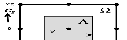
Figure 1: A two dimensional slice of the vacuum valley along the $(C_{1},C_{2})$ plane. The grey square is the fundamental domain $\Lambda$. The dots are gauge copies of the origin (which turn out to lie on the Gribov horizon $\Omega$, indicated by the fat square).

Also in the supersymmetric case, the Hamiltonian is invariant under anti-periodic gauge transformations (gauge transformations periodic up to an element of the center of the gauge group). When $\vec{n}$ has at least one of its components half integer it is homotopically non-trivial. Since it is a symmetry of the full Hamiltonian, this is one way to see that the vacuum valley has 8 orbifold singularities, related to $A=0$ by shifts over half-periods ($2\pi$ in each of the three directions). Alternatively, the action of the Weyl group on the vacuum valley is given by the reflection $\vec{C}\rightarrow-\vec{C}$, and the orbifold singularities are at the eight fixed points of this symmetry (combined with the shift symmetries). The cell $\vec{C}\in[-\pi,\pi]^{3}$ can be used as a fundamental domain $\Lambda$, see Fig. 1. Any point on the vacuum valley can be reached by applying suitable gauge transformations. Opposite sides on it’s boundary are identified under these homotopically non-trivial gauge transformations. The representations of their homotopy define the electric flux quantum numbers as introduced by ’t Hooft.$\!{}^{{\bf?}}$ We will here only consider the sector with zero electric flux, i.e. the trivial representation, where wave functions at opposite sides are equal.

We need to reconsider the construction of the effective Hamiltonian, since the gluino loops tend to cancel the gauge loops. For a background with zero field strength, the effective potential is easily seen to vanish to all orders in perturbation theory.$\!{}^{{\bf?}}$ But to resolve the orbifold singularity near $A=0$, we do not wish to integrate out the non-abelian zero-momentum modes. These modes can have non-zero field strength, and the quantum corrections for these are expected not all to cancel. Otherwise the $\beta$-function would vanish, which we know not to be the case for $N=1$ supersymmetric gauge theories. If necessary, field redefinitions should restore the supersymmetry.

In the background field gauge the one-loop effective potential reads

$$V_{1}(c)=L^{-1}\left\{\frac{1}{4}\left(\frac{L^{d-3}}{g_{0}^{2}}+\alpha_{2}(d)\right)(F^{a}_{ij})^{2}+\alpha_{3}(F^{a}_{ij})^{2}(c_{k}^{b})^{2}+\alpha_{5}{\det}^{2}(c)+\cdots\right\},$$ (5)

where $F^{a}_{ij}\equiv-\varepsilon_{abd}c_{j}^{b}c_{k}^{d}$. The coefficients (labeled as in the bosonic case $\!{}^{{\bf?}}$) in dimensional regularization are, up to terms vanishing at $d=3$, given by ($\vec{k}\in(2\pi{\rm Z\!\!Z})^{3}$)

$$\alpha_{2}(d)=-\frac{(d+3)(d+6)}{12d}\sum_{\vec{k}\neq\vec{0}}\frac{1}{|\vec{k}|^{3}},\ \alpha_{3}=-\frac{1}{32}\sum_{\vec{k}\neq\vec{0}}\frac{1}{|\vec{k}|^{5}},\ \alpha_{5}=-\frac{15}{16}\sum_{\vec{k}\neq\vec{0}}\frac{1}{|\vec{k}|^{5}}.$$ (6)

The result for dimensional reduction (vector and spinor indices strictly in 4 space-time dimensions) is simply obtained here (and below) by putting $d=3$, or $\!{}^{{\bf?}}$ $\alpha_{2}(3)=-\frac{3}{2}\sum_{\vec{k}\neq\vec{0}}|\vec{k}|^{-3}=\frac{3}{4\pi^{2}(d-3)}+\frac{3}{8\pi^{2}}\left(\frac{1}{11}+0.409052802\cdots\right)+{\cal O}(d-3)$. The effective potential vanishes along the vacuum valley, as expected.

In minimal subtraction one defines

$$\frac{L^{d-3}}{g_{0}^{2}}=-\frac{3}{4\pi^{2}(d-3)}+\frac{1}{g^{2}(L)},\quad\frac{1}{g^{2}(L)}\equiv-\frac{3}{4\pi^{2}}\ln(L\Lambda_{{}_{\rm MS}}),$$ (7)

such that $L^{d-3}/g_{0}^{2}+\alpha_{2}(d)=1/g^{2}(L)+\alpha_{2}$, with $\alpha_{2}$ the finite part of $\alpha_{2}(d)$, and $g(L)$ the running coupling appropriate for the supersymmetric theory. The “electric” part of the effective Lagrangian is also not difficult to compute in the background field calculation,

$${\scriptstyle{{1\over 2}}}L\left(\frac{L^{d-3}}{g_{0}^{2}}+\alpha_{1}(d)\right)\left((D_{0}c_{i})^{a}(t)\right)^{2},\quad\alpha_{1}(d)=-\frac{3+5d}{4d}\sum_{\vec{k}\neq\vec{0}}\frac{1}{|\vec{k}|^{3}}.$$ (8)

With $(D_{0}c_{i})^{a}=\dot{c}_{i}^{a}+\varepsilon_{adb}c_{0}^{d}c_{i}^{b}$, we keep $c^{a}_{0}\neq 0$ to preserve supersymmetry,

$$\delta A_{\mu}^{a}=\frac{i}{2}(\bar{\varepsilon}\gamma_{\mu}\lambda^{a}-{\bar{\lambda}}^{a}\gamma_{\mu}\varepsilon),\quad\delta\lambda^{a}=\gamma^{\mu\nu}F_{\mu\nu}^{a}\varepsilon,\quad\delta{\bar{\lambda}}^{a}=-\bar{\epsilon}\gamma^{\mu\nu}F_{\mu\nu}^{a},$$ (9)

which allows for a consistent truncation to the zero-momentum sector. Both in dimensional regularization and dimensional reduction the finite parts, $\alpha_{1,2}$, are equal and will be absorbed in the running coupling. Finally, for the gluino part of the effective Lagrangian we find

$$\frac{iZ}{2g_{0}^{2}}L^{d-1}{\bar{\lambda}}^{a}(t)\left(L\gamma_{0}\dot{\lambda}^{a}(t)+\kappa\varepsilon_{adb}c_{i}^{d}(t)\lambda^{b}(t)\right),\ Z=1+\frac{g_{0}^{2}}{2}\sum_{\vec{k}\neq\vec{0}}\frac{1}{|\vec{k}|^{3}},\ \kappa=1.$$ (10)

In the background field gauge only the gluino field requires a rescaling to restore the supersymmetry (with our use of component fields, implying the Wess-Zumino gauge, we do not maintain explicit supersymmetry, but the final results should of course not depend on this).

We also used the Lorentz gauge, which shifts the coefficients by $\!{}^{{\bf?}}$ $\delta\{\alpha_{1},\alpha_{2}\}=\{1,2\}\sum_{\vec{k}\neq\vec{0}}|\vec{k}|^{-3}$, $\delta\{\alpha_{3},\delta\alpha_{5}\}=\{\frac{7}{192},-\frac{57}{32}\}\sum_{\vec{k}\neq\vec{0}}|\vec{k}|^{-5}$. In addition $\delta Z_{2}=0$, and $\delta\kappa={\scriptstyle{{1\over 2}}}\alpha_{1}$. Infinities are absorbed by a simple rescaling of the gluon field, as guaranteed by gauge invariance. The changes in $\alpha_{3}$ and $\alpha_{5}$ can be absorbed by a finite but non-linear field redefinition.$\!{}^{{\bf?}}$ All we want to stress here is, like in the abelian case,$\!{}^{{\bf?}}$ that supersymmetry does not imply that the corrections (like $\alpha_{3}$ and $\alpha_{5}$) need to vanish, but a self-consistent calculation requires further terms in the effective action, involving a non-static background field (for the bosonic case most reliably done in a Hamiltonian setting $\!{}^{{\bf?}}$). The importance of these higher order terms will become clear later. To lowest order, one finds the Hamiltonian truncated to the zero-momentum sector, with the bare coupling replaced by the renormalized coupling.

The energy gap in the fluctuations transverse to the vacuum valley is easily read off from the Lagrangian. Close to the origin it is given by $2|\vec{C}|/L$. Integrating out transverse degrees of freedom is only reliable if the energy of the low-lying states is smaller than this gap. This energy behaves as $g^{2/3}(L)/L$ (as shown in the next section, rescaling $c$ with $g^{2/3}(L)$ makes the Hamiltonian proportional to $g^{2/3}(L)/L$). The gap in the transverse fluctuations thus becomes of this order where $|\vec{C}|$ is of order $g^{2/3}(L)$.

Consider a sphere of radius $g^{1/3}(L)$ around each orbifold singularities, beyond which the adiabatic approximation is accurate. There, the wave function can be reduced to the vacuum valley and, assuming indeed it has zero energy, it will be constant. (Note that the chosen parametrization of the vacuum valley is independent of $g(L)$ and $L$.) As long as $g(L)$ is small, we may assume the wave function in the neighborhood of the orbifold singularity to respect spherical symmetry. In the bosonic case, once the wave function spreads out over the vacuum valley, any spherical symmetry is quickly lost. In the supersymmetric case, however, the reduced wave function on the vacuum valley will become constant up to exponential corrections at distances much greater than $g^{2/3}(L)$ from the orbifold singularities, which are separated over a distance $2\pi$. (Rescaling $c$ with $g^{2/3}(L)$, the boundary of the sphere introduced above is at $g^{-1/3}(L)$, with the boundary of the fundamental domain and the other orbifold singularities an other factor $g^{-1/3}(L)$ removed from that.) Instead of insisting that the groundstate wave function is normalizable, we should rather insist on its projection to the vacuum valley to become constant. As long as the wave function is bounded everywhere, the issues of normalizability $\!{}^{{\bf?}}$ in the context of the supermembrane or M-theory $\!{}^{{\bf?}}$ applications, is therefore of no relevance here. But the challenge of explicitly constructing the ground state, of course, remains the same (a subtle difference will be pointed out later).

As we have argued, when the volume is small enough, we may assume the groundstate wave function of the effective Hamiltonian to be spherically symmetric. The boundary conditions at the boundary of the fundamental domain are replaced by requiring this wave function to approach a constant, after projecting to the vacuum valley. This projection is well defined, because at large separations from the origin, the wave function becomes exponentially localized transverse to the vacuum valley. Spherical symmetry near the orbifold singularities will dramatically simplify the analysis.

In the next section we will set up the zero-momentum supersymmetric Hamiltonian, and its reduction to the gauge invariant, spherically symmetric sector. This is not new,$\!{}^{{\bf?},{\bf?}}$ but we will be able to push it to the point where we can explicitly construct a complete basis of states that respect these symmetries. The Hamiltonian can be split into a “radial” and “angular” part, and our basis explicitly diagonalizes the angular part (“spherical harmonics”) in terms of invariant polynomials. This may be useful in a more general context.

2 The Hamiltonian

The conventions for the superalgebra we follow are those of Wess and Bagger.$\!{}^{{\bf?}}$ For the formulation of the supersymmetric Hamiltonian we follow to a large extent earlier work.$\!{}^{{\bf?},{\bf?},{\bf?}}$ We start from the supercharge operators,

$$Q_{\alpha}=\sigma^{j}_{\alpha{\dot{\beta}}}{\bar{\lambda}}_{a}^{\dot{\beta}}\left(-i\frac{\partial}{\partial V^{j}_{a}}-iB_{j}^{a}\right),\quad{\bar{Q}}_{\dot{\alpha}}=\lambda_{a}^{\beta}\sigma^{j}_{\beta{\dot{\alpha}}}\left(-i\frac{\partial}{\partial V_{j}^{a}}+iB_{j}^{a}\right),$$ (11)

with $V_{i}^{a}\equiv c_{i}^{a}/(g(L)L)$ and $\sigma^{j}=\tau^{j}$ (and $\sigma^{0}$ the unit) as $2\times 2$ matrices. Restricting to the zero-momentum modes, both the Weyl spinors $\lambda_{a}^{\beta}$ and ${\bar{\lambda}}_{a}^{\dot{\beta}}$ are constant. Lowering indices is done with $\epsilon_{\alpha\beta}=\epsilon_{{\dot{\alpha}}{\dot{\beta}}}=-i\tau_{2}$, $\delta_{ab}$ and $\eta_{\mu\nu}={\rm diag}(1,1,1,-1)$ (or $\delta_{ij}$) for respectively the spinor, group and space-time (or space) indices, and raising of indices is done with the inverse of these matrices. Repeated indices are assumed to be summed over, but to keep notations transparent we will not always balance the positions of the gauge and space indices. For zero-momentum gauge fields

$$B_{i}^{a}=-{\scriptstyle{{1\over 2}}}g\varepsilon_{ijk}\varepsilon_{abc}V_{j}^{b}V_{k}^{c}.$$ (12)

In the Hamiltonian formulation the anti-commutation relations

$$\{\lambda^{a\alpha},{\bar{\lambda}}^{b{\dot{\beta}}}\}={\bar{\sigma}}_{0}^{{\dot{\beta}}\alpha}\delta^{ab},\quad\{\lambda^{a\alpha},\lambda^{b\beta}\}=0,\quad\{{\bar{\lambda}}^{a{\dot{\alpha}}},{\bar{\lambda}}^{b{\dot{\beta}}}\}=0,$$ (13)

with ${\bar{\sigma}}_{0}$ the unit $2\times 2$ matrix (one has $({\bar{\sigma}}^{\mu})^{{\dot{\alpha}}\alpha}=\epsilon^{{\dot{\alpha}}{\dot{\beta}}}\epsilon^{\alpha\beta}(\sigma^{\mu})_{\beta{\dot{\beta}}}$), give

$$\{Q_{\alpha},{\bar{Q}}_{\dot{\alpha}}\}=2(\sigma_{0})_{\alpha{\dot{\alpha}}}{\cal H}-2(\sigma^{i})_{\alpha{\dot{\alpha}}}V_{i}^{a}{\cal G}_{a},$$ (14)

where

$${\cal G}_{a}=ig\varepsilon_{abc}\left(V_{j}^{c}\frac{\partial}{\partial V_{j}^{b}}-{\bar{\lambda}}^{b}{\bar{\sigma}}_{0}\lambda^{c}\right)$$ (15)

is the generator of infinitesimal gauge transformations, and ${\cal H}$ is the Hamiltonian density

$${\cal H}=-{\scriptstyle{{1\over 2}}}\frac{\partial^{2}}{\partial V_{i}^{a}\partial V_{i}^{a}}+{\scriptstyle{{1\over 2}}}B_{i}^{a}B_{i}^{a}-ig\varepsilon_{abc}{\bar{\lambda}}^{a}{\bar{\sigma}}^{j}\lambda^{b}V_{j}^{c}.$$ (16)

Splitting the Hamiltonian, $\int d^{3}x{\cal H}\equiv g^{2/3}(L)H/L$, in its bosonic and fermionic pieces, $H=H_{B}+H_{f}$, we find with $c_{i}^{a}=g^{2/3}(L){\hat{c}}_{i}^{a}$

$$H_{B}=-{\scriptstyle{{1\over 2}}}\left(\frac{\partial}{\partial{\hat{c}}_{i}^{a}}\right)^{2}+{\scriptstyle{{1\over 2}}}\left(\hat{B}_{i}^{a}\right)^{2},\quad H_{f}=-i\varepsilon_{abd}{\bar{\lambda}}^{a}{\bar{\sigma}}^{i}\lambda^{b}{\hat{c}}_{i}^{d},$$ (17)

where

$$\hat{B}^{i}_{a}=-{\scriptstyle{{1\over 2}}}\varepsilon^{ijk}\varepsilon_{abd}\hat{c}_{j}^{b}{\hat{c}}_{k}^{d}.$$ (18)

As discussed in the previous section, the orbifold singularities, other than at ${\hat{c}}=0$, lie at a distance $2\pi g^{-2/3}(L)$ in these new variables ${\hat{c}}$ (measured along the vacuum valley where $\hat{B}$ vanishes). We want to solve for the groundstate wave function such that for $|{\hat{c}}|\gg 1$ it becomes a constant, after projecting to the vacuum valley (we will come back to this projection later). As this boundary condition is compatible with spherical symmetry, i.e. it goes to the same constant for all directions on the vacuum valley, we will restrict ourselves to wave functions $\Psi({\hat{c}})$ that are spherically symmetric and gauge invariant. We stress this is an accidental spherical symmetry, that holds in sufficiently small volumes.

Building the Fock space of invariant states, we first separate in the fermion number. Sates with odd fermion number do not respect the symmetry and we can only $\!{}^{{\bf?}}$ have $F=0,2,4$ and 6 (there are six independent Weyl components). Particle-hole symmetry relates $F=0$ to $F=6$ and $F=2$ to $F=4$. Since $H_{f}|F=0\rangle=H_{f}|F=6\rangle=0$ (the diagonal entries of ${\bar{\sigma}}^{i}$ vanish), this case reduces to the bosonic Hamiltonian which is known not to have a zero vacuum energy.$\!{}^{{\bf?}}$ So we can restrict our attention to the $|F=2\rangle$ states. The index will be twice the number of zero-energy states in this sector (due to the particle-hole symmetry, see below). It should be noted that only the relative fermion number is well-defined, because integrating out certain modes involves filling negative energy (one-particle) gluino states.

2.1 Invariant two-gluino states

Instead of making irreducible decompositions of the variables,$\!{}^{{\bf?}}$ we chose to write down the most general $F=2$ states, and show how the Hamiltonian acts on these. We can combine two-spinors symmetric or antisymmetric in the gauge index (and thus respectively antisymmetric and symmetric in the spinor index)

$$|{\cal V}\rangle\equiv{{\cal V}_{j}}^{a}{{\cal I}^{j}}_{a}\equiv-2i{\cal V}_{j}^{c}\varepsilon_{abc}{\bar{\lambda}}^{a}_{\dot{\alpha}}({\bar{\sigma}}^{j0})^{\dot{\alpha}}_{\dot{\beta}}{\bar{\lambda}}^{b{\dot{\beta}}}|0\rangle,$$

$$|{\cal S}\rangle\equiv{\cal S}_{ab}{\cal J}^{ab}\equiv-{\cal S}_{ab}{\bar{\lambda}}^{a}_{\dot{\alpha}}{\bar{\lambda}}^{b}_{\dot{\beta}}\epsilon^{{\dot{\alpha}}{\dot{\beta}}}|0\rangle,$$ (19)

where ${\bar{\sigma}}^{\mu\nu}={\scriptstyle{{1\over 4}}}({\bar{\sigma}}^{\mu}\sigma^{\nu}-{\bar{\sigma}}^{\nu}\sigma^{\mu})$, such that ${\bar{\sigma}}^{j0}={\scriptstyle{{1\over 2}}}\tau_{j}$ as a $2\times 2$ matrix with the first index up and the second down (bringing also the first index down leads to a symmetric $2\times 2$ matrix). Here ${\cal V}_{j}^{a}$ and ${\cal S}^{ab}={\cal S}^{ba}$ are arbitrary (and assumed to depend on ${\hat{c}}_{i}^{a}$). The action of the Hamiltonian on these states preserves this structure

$$H_{f}(|{\cal S}\rangle+|{\cal V}\rangle)=|\tilde{\cal V}\rangle+|\tilde{\cal S}\rangle$$ (20)

with

$$\tilde{{\cal V}_{i}}^{a}=\varepsilon_{ijk}\varepsilon_{abd}{\hat{c}}_{j}^{b}{\cal V}_{k}^{d}+{\hat{c}}_{i}^{a}{\cal S}^{bb}-{\hat{c}}_{i}^{b}{\cal S}^{ba},$$

$$\tilde{\cal S}^{ab}=2\delta^{ab}{\hat{c}}_{i}^{d}{\cal V}_{i}^{d}-{\hat{c}}_{i}^{a}{\cal V}_{i}^{b}-{\hat{c}}_{i}^{b}{\cal V}_{i}^{a}.$$ (21)

Covariance allows us to write the most general form

$${{\cal V}_{j}}^{a}=h_{1}({\hat{r}},u,v){\hat{c}}_{j}^{a}/{\hat{r}}-h_{2}({\hat{r}},u,v)\hat{B}_{j}^{a}/{\hat{r}}^{2}+h_{3}({\hat{r}},u,v){\hat{c}}_{j}^{b}{\hat{c}}_{k}^{b}{\hat{c}}_{k}^{a}/{\hat{r}}^{3},$$

$${\cal S}^{ab}=h_{4}({\hat{r}},u,v)\delta^{ab}+h_{5}({\hat{r}},u,v){\hat{c}}_{j}^{a}{\hat{c}}_{j}^{b}/{\hat{r}}^{2}+h_{6}({\hat{r}},u,v){\hat{c}}_{j}^{a}{\hat{c}}_{j}^{d}{\hat{c}}_{k}^{d}{\hat{c}}_{k}^{b}/{\hat{r}}^{4},$$ (22)

in terms of the invariants ${\hat{r}}^{2}=({\hat{c}}_{j}^{a})^{2}$, $u={\hat{r}}^{-4}(\hat{B}_{j}^{a})^{2}$ and $v={\hat{r}}^{-3}\det{\hat{c}}$. It is useful to introduce the polar decomposition $\!{}^{{\bf?}}$ ${\hat{c}}_{i}^{a}=\sum_{j}R_{ij}x_{j}T^{ja}$, with $R,T\in SO(3)$, since the spherical symmetry and gauge invariance allows us to put ${\hat{c}}_{i}^{a}={\rm diag}(x_{1},x_{2},x_{3})$. Note that this does not completely fix the freedom under gauge and spatial rotations. The remnant symmetry involves permutations of the $x_{i}$ and simultaneously flipping two of its signs. In terms of $\vec{x}$, ${\hat{r}}^{2}=\sum_{j}x_{j}^{2}$, $u={\hat{r}}^{-4}\sum_{i>j}x_{i}^{2}x_{j}^{2}$ and $v={\hat{r}}^{-3}\prod_{j}x_{j}$, properly invariant under the remnant symmetry. Fixing this remnant symmetry, for example by $|x_{1}|\leq x_{2}\leq x_{3}$, allows one to solve the $x_{i}$ from $({\hat{r}},u,v)$. That ${\cal V}$ and ${\cal S}$ can be expanded each in terms of three invariant functions (the $h_{m}$) is most easily established in this diagonal representation

$${{\cal V}_{j}}^{a}=\delta_{j}^{a}\left(h_{1}({\hat{r}},u,v){\hat{r}}^{-1}x_{j}^{a}+h_{2}({\hat{r}},u,v){\hat{r}}^{-2}\det{\hat{c}}/x_{j}+h_{3}({\hat{r}},u,v){\hat{r}}^{-3}x_{j}^{3}\right),$$

$${\cal S}^{ab}=\delta^{ab}\left(h_{4}({\hat{r}},u,v)+h_{5}({\hat{r}},u,v){\hat{r}}^{-2}x_{a}^{2}+h_{6}({\hat{r}},u,v){\hat{r}}^{-4}x_{a}^{4}\right),$$ (23)

(note that $\hat{B}_{j}^{a}=-\delta_{j}^{a}x_{j}^{-1}\det{\hat{c}}$; no summations over repeated indices). Any higher order term can be reduced to this form. This is best illustrated by examples: one brings $\delta_{j}^{a}x_{j}^{5}$ and $\delta^{ab}x_{a}^{6}$ to the respective form of ${\cal V}^{a}_{j}$ and ${\cal S}^{ab}$ in Eq. (23), by using the identities $x_{j}^{5}={\hat{r}}^{2}x_{j}^{3}-{\hat{r}}^{4}ux_{j}+{\hat{r}}^{6}v^{2}/x_{j}$ and $x_{a}^{6}={\hat{r}}^{2}x_{a}^{4}-{\hat{r}}^{4}ux_{a}^{2}+{\hat{r}}^{6}v^{2}$.

We have established that any invariant state $|\Psi\rangle$ can be decomposed as

$$|\Psi\rangle=\sum_{m=1}^{6}h_{m}({\hat{r}},u,v)|e_{m}(u,v)\rangle,$$ (24)

where the $|e_{m}\rangle$ are implicitly defined by Eqs. (19,22). Since $H_{f}$ does not contain any derivatives with respect to ${\hat{c}}$, we can diagonalize $H_{f}$ pointwize. First determine the matrix of $H_{f}$ with respect to the basis $|e_{m}\rangle$

$$H_{f}|e_{m}\rangle=\sum_{n=1}^{6}|e_{n}\rangle H_{f}^{nm}.$$ (25)

From Eq. (21) one directly reads off that

$$H_{f}^{mn}={\hat{r}}\pmatrix{0&1&-v&2&1&1-u\cr 2&0&1&0&0&-v\cr 0&-1&0&0&-1&-1\cr 2&4v&2-4u&0&0&0\cr-2&0&0&0&0&0\cr 0&0&-2&0&0&0\cr}.$$ (26)

This matrix is not symmetric due to the fact that the $|e_{m}\rangle$ are in general not orthogonal. The non-diagonal norm matrix $N^{mn}\equiv\langle e_{m}|e_{n}\rangle$ is however block diagonal, since $\langle{\cal S}|{\cal V}\rangle=0$ for any choice of ${\cal V}$ and ${\cal S}$. Introducing the notation $X=1-2u$, $Y=1-3u+3v^{2}$, $Z=1+2u^{2}-4u+4v^{2}$ one finds

$$N^{mn}=\pmatrix{8&24v&8X&0&0&0\cr 24v&8u&8v&0&0&0\cr 8X&8v&8Y&0&0&0\cr 0&0&0&12&4&4X\cr 0&0&0&4&4X&4Y\cr 0&0&0&4X&4Y&4Z\cr}.$$ (27)

The matrix $N$ can be used to make an orthonormal basis. It transforms $H_{f}$ to $N^{{\scriptstyle{{1\over 2}}}}\cdot H_{f}\cdot N^{-{\scriptstyle{{1\over 2}}}}$. This is seen to be symmetric, e.g. by establishing the symmetry of $N\cdot H_{f}$.

Figure 2: The six eigenvalues $E_{f}/{\hat{r}}$, of $H_{f}/{\hat{r}}$, plotted versus $3v\sqrt{3}$.

We denote by $E_{f}$ the energies of the two-gluino state in a given background. With $E_{f}$ linear in ${\hat{r}}$ and, as we will see, independent of $u$, only the $v$ dependence is non-trivial. The eigenvalues of $H_{f}$, for the six invariant two-gluino states, are determined by

$$\det(H_{f}-E_{f})=(E_{f}^{3}-4{\hat{c}}^{2}E_{f}-16\det{\hat{c}})(E_{f}^{3}-{\hat{c}}^{2}E_{f}+2\det{\hat{c}})=0,$$ (28)

In terms of the three roots $\mu_{i}$, $E_{f}^{3}-{\hat{c}}^{2}E_{f}+2\det{\hat{c}}=(E_{f}-\mu_{1})(E_{f}-\mu_{2})(E_{f}-\mu_{3})$, the remaining three roots are given by $\tilde{\mu}_{i}=-2\mu_{i}$. Note that $\sum_{i}\mu_{i}=0$, $\sum_{i}\mu_{i}^{2}=2{\hat{c}}^{2}$ and $\prod_{i}\mu_{i}=-2\det{\hat{c}}$. Explicit expressions for the two-gluino energies are (see Fig. 2)

$$\tilde{\mu}_{k}=-2\mu_{k}=-4{\hat{r}}\cos(2\pi k/3+\arccos[-3v\sqrt{3}]/3)/\sqrt{3},$$ (29)

with $\arccos$ ranging from 0 to $\pi$. Note that $3v\sqrt{3}\in[-1,1]$ since $\prod x_{i}$ is extremal (under the constraint $\sum_{i}x_{i}^{2}=1$) when all $|x_{i}|$ are equal (to $1/\sqrt{3}$). The lowest eigenvalue, $E^{\rm min}_{f}\equiv\tilde{\mu}_{3}$, takes on the value $-2{\hat{r}}$ along the vacuum valley, since $u=0$ implies $v=0$. The eigenvectors associated to the eigenvalue $\tilde{\mu}_{k}$ are also easily constructed,

$$\tilde{h}^{(k)}=\left({\scriptstyle{{1\over 2}}}\tilde{\mu}_{k}/{\hat{r}},1,0,1+4v{\hat{r}}/\tilde{\mu}_{k},-1,0\right)/|4(1+6v{\hat{r}}/\tilde{\mu}_{k})|,$$ (30)

normalized in a fixed background according to $\sum_{m,n=1}^{6}\tilde{h}_{m}^{(k)}N^{mn}\tilde{h}^{(k^{\prime})}_{n}=\delta_{kk^{\prime}}$. We will not write down the more complicated analytic form for the eigen functions belonging to the remaining three eigenvalues. Only $\tilde{h}^{(3)}$ will be referred to later when discussing projection to the vacuum valley.

At this point it is perhaps interesting to observe that along the vacuum valley (two out of the three $x_{j}$ vanish), the particle-hole dual of $|\Psi\rangle=\tilde{h}^{(3)}_{m}|e_{m}\rangle$ can be expressed as $|\bar{\Psi}\rangle={\scriptstyle{{1\over 2}}}{\bar{\lambda}}_{\dot{\alpha}}^{a}{\hat{c}}_{i}^{a}{\hat{c}}_{i}^{b}{\bar{\lambda}}_{b}^{\dot{\alpha}}|\Psi\rangle$, obtained from $|\Psi\rangle$ by creating a pair of abelian zero-momentum gluinos, in accordance with the analysis of Witten.$\!{}^{{\bf?}}$ To prove this, note that with ${\hat{c}}_{i}^{a}$ abelian, defining ${\cal V}_{i}^{a}=-{\hat{c}}_{i}^{a}$ and ${\cal S}_{ab}=\delta_{ab}-{\hat{c}}_{i}^{a}{\hat{c}}_{i}^{b}$, we can write $|\Psi\rangle=|{\cal V}\rangle+|{\cal S}\rangle$. Its particle-hole dual is given by $|\bar{\Psi}\rangle=|\bar{{\cal V}}\rangle+|\bar{{\cal S}}\rangle$, with

$$|\bar{{\cal V}}\rangle\equiv{{\cal V}_{j}}^{a}{\bar{{\cal I}}^{j}}_{a}\equiv-2i{\cal V}_{j}^{c}\varepsilon_{abc}\lambda^{a}_{\alpha}(\sigma^{j0})^{\alpha}_{\beta}\lambda^{b\beta}|\bar{0}\rangle,$$

$$|\bar{{\cal S}}\rangle\equiv{\cal S}_{ab}{\hat{c}}\bar{J}^{ab}\equiv-{\cal S}_{ab}\lambda^{a}_{\alpha}\lambda^{b}_{\beta}\epsilon^{\alpha\beta}|\bar{0}\rangle,\quad|\bar{0}\rangle\equiv\prod_{a{\dot{\alpha}}}{\bar{\lambda}}_{\dot{\alpha}}^{a}|0\rangle,$$ (31)

also defining the particle-hole symmetry in the general case.

It should be noted that our change of variables from ${\hat{c}}$ to $x_{i}$ will suffer from coordinate singularities, also affecting the linear independence of the $|e_{m}\rangle$. This is most obvious from the fact that $\det N=32768J^{4}$, with $J$ (up to a constant) the Jacobian for the change of variables, $d^{9}{\hat{c}}={\scriptstyle{{2\over 3}}}\pi^{4}Jd^{3}x$ (with $|x_{1}|\leq x_{2}\leq x_{3}$),

$$J\equiv\prod_{i>j}^{\vphantom{j}}|x_{i}^{2}-x_{j}^{2}|={\hat{r}}^{6}\sqrt{u^{2}(1-4u)-v^{2}(4-18u+27v^{2})}.$$ (32)

Indeed, the normalization of $\tilde{h}^{(k)}$ in Eq. (30) is singular when $\tilde{\mu}_{k}+6v{\hat{r}}$ vanishes, which is easily identified with a vanishing Jacobian. For this observe that $3{\hat{c}}^{2}E_{f}+18\det{\hat{c}}=3{\hat{r}}^{2}(E_{f}+6v{\hat{r}})$ equals the difference of $E_{f}^{3}-4{\hat{c}}^{2}E_{f}-16\det{\hat{c}}$ and $E_{f}^{3}-{\hat{c}}^{2}E_{f}+2\det{\hat{c}}$. Since each of these vanish for either $E_{f}=\tilde{\mu}_{i}$ or $E_{f}=\mu_{i}$, we conclude that $\tilde{\mu}_{k}+6v{\hat{r}}$ vanishes if and only if $\tilde{\mu}_{k}$ coincides with one of the other roots $\mu_{i}$. From Fig. 2 we read off this happens for $v=\pm\sqrt{3}/9$, which is the extremal value of $v$ where all three $|x_{i}|$ are equal (constraining $u$ to be $3|v|^{4/3}=1/3$), and therefore $J=0$. As long as $J\neq 0$, the limit $v\rightarrow 0$ exists, e.g.

$$\lim_{v\rightarrow 0}\pmatrix{\tilde{h}^{(1)}\cr\tilde{h}^{(2)}\cr\tilde{h}^{(3)}\cr}=\pmatrix{{\scriptstyle{{1\over 4}}}&{\scriptstyle{{1\over 4}}}&0&{\scriptstyle{{1\over 4}}}&-{\scriptstyle{{1\over 4}}}&0\cr 0&{\scriptstyle{{1\over 2}}}&0&0&-{\scriptstyle{{1\over 2}}}&0\cr-{\scriptstyle{{1\over 4}}}&{\scriptstyle{{1\over 4}}}&0&{\scriptstyle{{1\over 4}}}&-{\scriptstyle{{1\over 4}}}&0\cr},$$ (33)

independent of $u$, but we have to remember that when $J=0$ (in particular $u=0$) the $|e_{m}\rangle$ are no longer independent. We come back to this when projecting to the vacuum valley.

Before constructing a full invariant basis, to gain more confidence that the $|e_{m}\rangle$ correctly describe the invariant two-gluino states, it is useful to note that the spectrum of $H_{f}$ can also be obtained from its (non-invariant) one-particle states.$\!{}^{{\bf?}}$ For this we write

$$H_{f}={\bar{\lambda}}^{a}_{\dot{\alpha}}M^{{\dot{\alpha}}\beta}_{ab}\lambda^{b}_{\beta},\quad M^{{\dot{\alpha}}\beta}_{ab}=-i\varepsilon_{abd}({\bar{\sigma}}^{j})^{{\dot{\alpha}}\beta}{\hat{c}}_{j}^{d}.$$ (34)

The one-particle fermion energies are given by the eigenvalues of $M$. Note that charge conjugation symmetry, $M^{*}=\tau_{2}M\tau_{2}$, implies each eigenvalue is two-fold degenerate. By direct computation one verifies that $\!{}^{{\bf?}}$

$$M^{3}-{\hat{c}}^{2}M-2\det{\hat{c}}=0,$$ (35)

such that any eigenvalue $\mu$ of $M$ satisfies the equation $\mu^{3}-{\hat{c}}^{2}\mu-2\det{\hat{c}}=(\mu+\mu_{1})(\mu+\mu_{2})(\mu+\mu_{3})=0$, with $\mu_{i}$ as defined before. Hence the one-particle fermion energies are given by $-\mu_{i}$, and each occurs with a two-fold (spin) degeneracy. We can make invariant two-particle states only by combining two opposite spin states. There are six such invariant states, three with the same one-particle energies, giving $E_{f}=-2\mu_{i}=\tilde{\mu}_{i}$, and three with different one-particle energies, giving $E_{f}=-\mu_{i}-\mu_{j}=\mu_{k}$ with $i\neq j\neq k$. This agrees with our earlier results. Note that there are also three triplet two-gluino states with two-particle energies $E_{f}=\mu_{k}$, combining two one-particle states with different energies but equal spin, which are not invariant and thus left out from our considerations. See the Appendix for yet another method.

2.2 Supersymmetric spherical harmonics

We have removed the angular degrees of freedom on which the invariant wave functions do not depend: those associated with the gauge and space rotations. This leaves a six component $F=2$ wave function, depending on either $({\hat{r}},u,v)$ or equivalently $(x_{1},x_{2},x_{3})$. It is well known $\!{}^{{\bf?},{\bf?}}$ that the kinetic term of the Hamiltonian reduces to

$$-{\scriptstyle{{1\over 2}}}\frac{\partial^{2}}{(\partial{\hat{c}}_{i}^{a})^{2}}=-{\scriptstyle{{1\over 2}}}J^{-1}(\vec{x})\frac{\partial}{\partial x_{j}}J(\vec{x})\frac{\partial}{\partial x_{j}}=-{\scriptstyle{{1\over 2}}}\left({\hat{r}}^{-8}\frac{\partial}{\partial{\hat{r}}}{\hat{r}}^{8}\frac{\partial}{\partial{\hat{r}}}+\frac{\Delta(u,v)}{{\hat{r}}^{2}}\right),$$ (36)

with $\Delta(u,v)$ the Laplacian for $S^{8}$, acting on invariant functions, given by $\!{}^{{\bf?}}$

$$\Delta(u,v) = 4(3v^{2}+u-4u^{2})\frac{\partial^{2}}{(\partial u)^{2}}+8(1-3u)v\frac{\partial^{2}}{\partial u\partial v}+(u-9v^{2})\frac{\partial^{2}}{(\partial v)^{2}}$$ (37)

$$+4(2-11u)\frac{\partial}{\partial u}-30v\frac{\partial}{\partial v}.$$

Note that for the bosonic theory ($F=0$) the variables $({\hat{r}},u,v^{2})$ were used (for the positive parity states), but for the $F=2$ sector functions even and odd in $v$ mix, requiring us to use the variables $({\hat{r}},u,v)$. The Hamiltonian still allows for a radial decomposition (note that $\partial_{\hat{r}}|e_{m}\rangle=0$)

$$\hat{H}^{mn}=-{\scriptstyle{{1\over 2}}}\delta^{mn}{\hat{r}}^{-8}\frac{\partial}{\partial{\hat{r}}}{\hat{r}}^{8}\frac{\partial}{\partial{\hat{r}}}+{\scriptstyle{{1\over 2}}}\delta^{mn}{\hat{r}}^{4}u+{\hat{r}}\hat{H}_{f}^{mn}+{\hat{r}}^{-2}\hat{H}_{\Delta}^{mn},$$ (38)

where $\hat{H}_{f}^{mn}\equiv H_{f}^{mn}/{\hat{r}}$, see Eq. (26), and

$$\sum_{m,n=1}^{6}|e_{n}(u,v)\rangle\hat{H}_{\Delta}^{nm}h_{m}({\hat{r}},u,v)=-{\scriptstyle{{1\over 2}}}\Delta(u,v)\sum_{m=1}^{6}h_{m}({\hat{r}},u,v)|e_{m}(u,v)\rangle.$$ (39)

It is straightforward, but quite tedious, to explicitly calculate $\hat{H}_{\Delta}^{mn}$,

$$\hat{H}^{mn}_{\Delta}=-{\scriptstyle{{1\over 2}}}\delta^{mn}\Delta(u,v)-{\scriptstyle{{1\over 2}}}\pmatrix{\Delta^{1}_{\cal V}&\oslash\cr\oslash&\Delta^{1}_{\cal S}\cr}-{\scriptstyle{{1\over 2}}}\pmatrix{\Delta^{0}_{\cal V}&\oslash\cr\oslash&\Delta^{0}_{\cal S}\cr}.$$ (40)

For the first term $\Delta$ only acts on the coefficient functions, for the next we collect the terms where one derivative acts on the coefficient functions and one on the two-gluino basis vectors $|e_{m}\rangle$, whereas the last term has all derivatives acting on these basis vectors. This splits in the two sectors associated to $|{\cal V}\rangle$ and $|{\cal S}\rangle$, since derivatives cannot lead to mixing of these two-gluino states, specified by ${\cal I}$ and ${\cal J}$ in Eq. (19). We find the following results

$$\Delta^{1}_{\cal V}\equiv 2\pmatrix{(2-4u)\partial_{u}-3v\partial_{v}&\partial_{v}+2v\partial_{u}&3v\partial_{v}+6u\partial_{u}\cr\partial_{v}&(2-8u)\partial_{u}-6v\partial_{v}&-6v\partial_{u}\cr-2\partial_{u}&-\partial_{v}&-12u\partial_{u}-9v\partial_{v}\cr},$$ (41)

$$\Delta^{1}_{\cal S}\equiv 2\pmatrix{0&2v\partial_{v}&-8v^{2}\partial_{u}\cr 0&(4-8u)\partial_{u}-6v\partial_{v}&4v\partial_{v}+8u\partial_{u}\cr 0&-4\partial_{u}&-16u\partial_{u}-12v\partial_{v}\cr},$$ (42)

and

$$\Delta^{0}_{\cal V}\equiv 2\pmatrix{\!-4&~{}0&~{}7\cr~{}0&\!-9&~{}0\cr~{}0&~{}0&\!-15\cr},\quad\Delta^{0}_{\cal S}\equiv\pmatrix{~{}0&~{}3&~{}1\cr~{}0&\!-9&~{}11\cr~{}0&~{}0&\!-22\cr}.$$ (43)

Invariant wave functions, $|\Psi\rangle=\sum_{m=1}^{6}h_{m}({\hat{r}},u,v)|e_{m}(u,v)\rangle$, are normalized using

$$\langle\Psi|\Psi^{\prime}\rangle=\int d^{9}{\hat{c}}\sum_{m,n=1}^{6}h^{*}_{m}N^{mn}h^{\prime}_{n},$$ (44)

with $N^{mn}$ the norm matrix as defined in Eq. (27). The matrix elements of the Hamiltonian with respect to such a basis are thus given by

$$\langle\Psi|H|\Psi^{\prime}\rangle=\int d^{9}{\hat{c}}\sum_{m,n,p=1}^{6}h^{*}_{m}N^{mn}\hat{H}^{np}h^{\prime}_{p},$$ (45)

with $\hat{H}^{mn}$ the matrix operator as defined in Eq. (38).

Like for the bosonic case (with $\hat{H}_{\Delta}\equiv-{\scriptstyle{{1\over 2}}}\Delta$ and $\hat{H}_{f}\equiv 0$) we first construct an invariant set of “angular” wave functions as polynomials in $u$ and $v$. These can be chosen to be eigenfunctions (${\cal Y}_{s}^{xyz}$) of $\hat{H}_{\Delta}$, proportional to coefficient functions $U_{s}^{z}$ defined by (for $F=0:\,z=0;\,s\in\{2,5\}$ and $F=2:\,z\in\{1,2,3\};$ $s\in\{0,1,2,3\}$)

$$\pmatrix{U^{1}_{0}\cr U^{2}_{0}\cr U^{3}_{0}\cr}=\pmatrix{0&0&0&1&0&0\cr 0&0&0&0&1&0\cr 0&0&0&0&0&1\cr} \pmatrix{U^{1}_{1}\cr U^{2}_{1}\cr U^{3}_{1}\cr}=\pmatrix{1&0&0&0&0&0\cr 0&0&1&0&0&0\cr 0&v&0&0&0&0\cr},$$ ,

$$\pmatrix{U^{1}_{2}\cr U^{2}_{2}\cr U^{3}_{2}\cr}=\pmatrix{0&1&0&0&0&0\cr v&0&0&0&0&0\cr 0&0&v&0&0&0\cr} \quad U^{z}_{3}=vU^{z}_{0},\quad U_{5}^{0}=vU_{2}^{0}=v,$$ , (46)

judiciously chosen such that $q=2x+3y+z$ allows us to order states, and

$$\hat{H}_{\Delta}u^{x}v^{2y}U_{s}^{z}={\scriptstyle{{1\over 2}}}(2q+s-2)(2q+s+5)u^{x}v^{2y}U_{s}^{z}+\delta R_{s}^{xyz},$$ (47)

with $\delta R_{s}^{xyz}$ a linear combination of these monomials, but of lower order in $q$ (states with different $s$ do not mix under $\hat{H}_{\Delta}$, but they do mix under $\hat{H}_{f}$). The appearance of the combination $2x+3y$ is related to the fact that $u^{x}v^{2y}=r^{-2(2x+3y)}(\hat{B}^{2})^{x}(\det{\hat{c}})^{2y}$. The eigenvalues of $\hat{H}_{\Delta}$ can be written as $L(2L+7)$, with the “angular momentum” $L=q+s/2-1=2x+3y+z+s/2-1$ taking half integer values. Eq. (47) allows us to solve $[\hat{H}_{\Delta}-L(2L+7)]{\cal Y}_{s}^{xyz}=0$ for $R_{s}^{xyz}$ (of order $q<2x+3y+z$), with

$${\cal Y}_{s}^{xyz}\equiv u^{x}v^{2y}U_{s}^{z}+R_{s}^{xyz}.$$ (48)

Table 1: All orthonormal spherical harmonics for $L<4$, with $L=2x+3y+z+s/2-1$, such that $\hat{H}_{\Delta}\hat{\cal Y}_{s}^{xyz}=L(2L+7)\hat{\cal Y}_{s}^{xyz}$. For higher $L$ use the available program.$\!{}^{{\bf?}}$

$L$	$\hat{\cal Y}_{n{\hphantom{0}}}\!=\hat{\cal Y}_{s}^{xyz}\!=(h_{1},h_{2},h_{3},h_{4},h_{5},h_{6})$
$0$	$\hat{\cal Y}_{1{\hphantom{0}}}=\hat{\cal Y}_{0}^{001}=(0,0,0,1,0,0)\sqrt{35/2}/8\pi^{2}$
${\scriptstyle{{1\over 2}}}$	$\hat{\cal Y}_{2{\hphantom{0}}}=\hat{\cal Y}_{1}^{001}=(1,0,0,0,0,0)\sqrt{105}/16\pi^{2}$
$1$	$\hat{\cal Y}_{3{\hphantom{0}}}=\hat{\cal Y}_{2}^{001}=(0,1,0,0,0,0)\sqrt{1155/2}/16\pi^{2}$
$1$	$\hat{\cal Y}_{4{\hphantom{0}}}=\hat{\cal Y}_{0}^{002}=(0,0,0,-\frac{1}{3},1,0)3\sqrt{77}/16\pi^{2}$
${\scriptstyle{{3\over 2}}}$	$\hat{\cal Y}_{5{\hphantom{0}}}=\hat{\cal Y}_{3}^{001}=(0,0,0,v,0,0)\sqrt{15015}/16\pi^{2}$
${\scriptstyle{{3\over 2}}}$	$\hat{\cal Y}_{6{\hphantom{0}}}=\hat{\cal Y}_{1}^{002}=(-\frac{7}{11},0,1,0,0,0)11\sqrt{273/5}/32\pi^{2}$
$2$	$\hat{\cal Y}_{7{\hphantom{0}}}=\hat{\cal Y}_{2}^{002}=(v,-\frac{1}{13},0,0,0,0)39\sqrt{77}/32\pi^{2}$
$2$	$\hat{\cal Y}_{8{\hphantom{0}}}=\hat{\cal Y}_{0}^{003}=(0,0,0,\frac{10}{143},-\frac{11}{13},1)429\sqrt{7/86}/16\pi^{2}$
$2$	$\hat{\cal Y}_{9{\hphantom{0}}}=\hat{\cal Y}_{0}^{101}=(0,0,0,-\frac{6}{43}+u,-\frac{22}{43},\frac{26}{43})3\sqrt{6149/2}/16\pi^{2}$
${\scriptstyle{{5\over 2}}}$	$\hat{\cal Y}_{10}=\hat{\cal Y}_{3}^{002}=(0,0,0,-\frac{v}{3},v,0)3\sqrt{51051/2}/16\pi^{2}$
${\scriptstyle{{5\over 2}}}$	$\hat{\cal Y}_{11}=\hat{\cal Y}_{1}^{003}=(-\frac{11}{195},v,\frac{1}{15},0,0,0)39\sqrt{1785}/64\pi^{2}$
${\scriptstyle{{5\over 2}}}$	$\hat{\cal Y}_{12}=\hat{\cal Y}_{1}^{101}=(-\frac{1}{4}+u,-\frac{13v}{44},\frac{5}{44},0,0,0)33\sqrt{221/7}/16\pi^{2}$
$3$	$\hat{\cal Y}_{13}=\hat{\cal Y}_{2}^{003}=(-\frac{10v}{17},\frac{1}{51},v,0,0,0)51\sqrt{4389/5}/32\pi^{2}$
$3$	$\hat{\cal Y}_{14}=\hat{\cal Y}_{2}^{101}=(-\frac{6v}{13},-\frac{12}{65}+u,\frac{38v}{65},0,0,0)39\sqrt{17765/7}/64\pi^{2}$
$3$	$\hat{\cal Y}_{15}=\hat{\cal Y}_{0}^{011}=(0,0,0,\frac{4}{663}-\frac{u}{17}+v^{2},0,0)663\sqrt{209/7}/32\pi^{2}$
$3$	$\hat{\cal Y}_{16}=\hat{\cal Y}_{0}^{102}=(0,0,0,\frac{2}{51}-\frac{3u}{17},-\frac{6}{17}+u,\frac{4}{17})51\sqrt{2717/7}/32\pi^{2}$
${\scriptstyle{{7\over 2}}}$	$\hat{\cal Y}_{17}=\hat{\cal Y}_{3}^{003}=(0,0,0,\frac{28v}{323},-\frac{15v}{19},v)969\sqrt{231/10}/32\pi^{2}$
${\scriptstyle{{7\over 2}}}$	$\hat{\cal Y}_{18}=\hat{\cal Y}_{3}^{101}=(0,0,0,-\frac{12v}{65}+uv,-\frac{6v}{13},\frac{38v}{65})39\sqrt{53295/2}/32\pi^{2}$
${\scriptstyle{{7\over 2}}}$	$\hat{\cal Y}_{19}=\hat{\cal Y}_{1}^{011}=(\frac{10}{969}-\frac{u}{19}+v^{2},-\frac{2v}{19},-\frac{2}{323},0,0,0)969\sqrt{429/14}/32\pi^{2}$
${\scriptstyle{{7\over 2}}}$	$\hat{\cal Y}_{20}=\hat{\cal Y}_{1}^{102}=(\frac{44}{399}-\frac{93u}{133}+\frac{2v^{2}}{7},\frac{2v}{7},-\frac{20}{133}+u,0,0,0)19\sqrt{51051/2}/64\pi^{2}$

To order these states at degenerate values of $L$, we begin at $L=0$ with ${\cal Y}_{1}={\cal Y}_{0}^{001}$. Raising $L$ with ${\scriptstyle{{1\over 2}}}$ we start with the lowest value of $q$ and construct the independent, but in general non-orthogonal states ${\cal Y}_{s}^{xyz}$. Using that $y$ and $z$ are uniquely fixed by $q-2x$, we start with $x=0$ and every time we increase $x$ by one, we modify ${\cal Y}_{s}^{xyz}$ by projecting it on the orthogonal complement of the previous states (the Gramm-Schmidt procedure). When completed we increase $q$ until all states with a given value of $L$ are constructed, after which we increase $L$. Dividing by the norm we thus obtain a complete orthonormal set of “spherical harmonics”, $\hat{\cal Y}_{n}(u,v)\equiv\langle u,v|n\rangle$, with $n$ labelling the $n$-th state thus constructed. The first few spherical harmonics $\hat{\cal Y}_{n}(u,v)$ are collected in Table 1. Note that to evaluate inner products we need to compute the integrals $X_{x,y}\equiv\int_{{\hat{r}}=1}d^{9}{\hat{c}}~{}u^{x}v^{2y}$. For this we recall the recursive definition $\!{}^{{\bf?}}$

$$X_{i,j}=\frac{4i(1+i+4j)X_{i-1,j}+12i(i-1)X_{i-2,j+1}+2j(2j-1)X_{i+1,j-1}}{(4i+6j)(4i+6j+7)},$$ (49)

with $X_{0,0}=32\pi^{4}/105$. The Mathematica $\!{}^{{\bf?}}$ code for generating the $\hat{\cal Y}_{n}$ is available through the World Wide Web.$\!{}^{{\bf?}}$

We denote by $L_{n}$ the value of $L=2x+3y+z+s/2-1$ implicitly defined by $\hat{\cal Y}_{n}=\hat{\cal Y}_{s}^{xyz}$. It will be convenient to also introduce $\ell\equiv 2L+3$. With the spherical harmonics we can now construct a reduced Hamiltonian,

$$\langle n^{\prime}|H|n\rangle=H^{n^{\prime}n}({\hat{r}})=K({\hat{r}};L_{n})\delta^{n^{\prime}n}+{\scriptstyle{{1\over 2}}}{\hat{r}}^{4}\langle n^{\prime}|u|n\rangle+{\hat{r}}\langle n^{\prime}|\hat{H}_{f}|n\rangle,$$

$$K({\hat{r}};L)=-{\scriptstyle{{1\over 2}}}{\hat{r}}^{-8}\partial_{\hat{r}}{\hat{r}}^{8}\partial_{\hat{r}}+{\hat{r}}^{-2}L(2L+7)={\hat{r}}^{-3}{\hat{K}}({\hat{r}},\ell){\hat{r}}^{3},$$

$${\hat{K}}({\hat{r}};\ell)=-{\scriptstyle{{1\over 2}}}{\hat{r}}^{-2}\partial_{\hat{r}}{\hat{r}}^{2}\partial_{\hat{r}}+{\scriptstyle{{1\over 2}}}{\hat{r}}^{-2}\ell(\ell+1).$$ (50)

We illustrate its sparse nature by showing in Fig. 3 the entries where either $\langle n^{\prime}|u|n\rangle\neq 0$ or $\langle n^{\prime}|\hat{H}_{f}|n\rangle\neq 0$ as black squares. The different bands can be traced to come from the selection rules $|\delta L|=0,1,2$ for the matrix elements of $u$, and $|\delta L|={\scriptstyle{{1\over 2}}}$ for the matrix elements of $\hat{H}_{f}$. The number of codiagonals is bound by $-3+4\sqrt{n}$.

Figure 3: Band structure of the reduced Hamiltonian, for the first 100 states.

To write down the matrix of the full Hamiltonian with respect to an invariant basis, we introduce radial wave functions $\phi_{p}^{\ell}({\hat{r}})\equiv\langle{\hat{r}}|p,\ell\rangle$. The radial quantum number $p$ is associated to a momentum if we choose

$$\phi_{p}^{\ell}({\hat{r}})=C_{p}^{\ell}{\hat{r}}^{-3}j_{\ell}(k^{\ell}_{p}{\hat{r}}),\quad E_{p}^{\ell}={\scriptstyle{{1\over 2}}}(k_{p}^{\ell})^{2},$$ (51)

where $j_{\ell}(z)$ is the spherical Bessel function which satisfies the equation ${\hat{K}}({\hat{r}};\ell)j_{\ell}({\hat{r}})={\scriptstyle{{1\over 2}}}j_{\ell}({\hat{r}})$ or $K({\hat{r}};L)\phi_{p}^{2L+3}({\hat{r}})=E_{p}^{2L+3}\phi_{p}^{2L+3}({\hat{r}})$. Normalization with a factor $C_{p}^{\ell}$ is such that $\int d{\hat{r}}~{}{\hat{r}}^{8}\phi_{p}^{\ell}({\hat{r}})^{*}\phi_{q}^{\ell}({\hat{r}})=\delta_{pq}$. In terms of the normalized basis of invariant states $\langle{\hat{c}}|p,n\rangle\equiv\langle u,v|n\rangle\langle{\hat{r}}|p,\ell_{n}\rangle$, the matrix of the Hamiltonian is given by $H_{n^{\prime}n}^{p^{\prime}p}=\langle p^{\prime},n|H|p,n\rangle$, or

$$H_{n^{\prime}n}^{p^{\prime}p}=E_{p}^{\ell_{n}}\delta_{nn^{\prime}}\delta^{pp^{\prime}}+\langle p^{\prime},\ell_{n^{\prime}}|{\hat{r}}^{4}|p,\ell_{n}\rangle\langle n^{\prime}|\frac{u}{2}|n\rangle+\langle p^{\prime},\ell_{n^{\prime}}|{\hat{r}}|p,\ell_{n}\rangle\langle n^{\prime}|\hat{H}_{f}|n\rangle.$$ (52)

To complete the construction of the basis, we need to address the question of boundary conditions (fixing the momenta), which somehow have to incorporate that the groundstate wave function becomes a constant, after projecting to the vacuum valley.

3 Vacuum valley and boundary condition

The vacuum valley is characterized by those configurations for which $u=0$ (this implies $v=0$), and ${\hat{r}}$ measures the (three-dimensional) distance to the origin along this vacuum valley. The wave function can be decomposed as $\Psi=\sum_{n=0}^{\infty}{\hat{r}}^{-3}f_{n}({\hat{r}})\chi_{n}(u,v;{\hat{r}})$, with $\chi_{n}(u,v;{\hat{r}})$ normalized eigenfunctions of ${\hat{H}_{\perp}}(u,v;{\hat{r}})=\hat{H}(u,v,{\hat{r}})|_{\partial_{\hat{r}}=0}$, see Eq. (38). It is convenient to use the spherical coordinates

$$\vec{x}={\hat{r}}\left(\sin(\varphi)\sin(\theta),\cos(\varphi)\sin(\theta),\cos(\theta)\right),$$ (53)

$$u=\sin^{2}\theta(\cos^{2}\theta+\cos^{2}\varphi\sin^{2}\varphi\sin^{2}\theta),\quad v=\sin^{2}\theta\cos^{2}\theta\cos\varphi\sin\varphi,$$

$$J={\hat{r}}^{6}|{\tilde{J}}|,\quad{\tilde{J}}=\sin^{2}\theta\cos(2\varphi)\left(1-3\sin^{2}\theta+\sin^{4}\theta[17-\cos(4\varphi)]/8\right),$$

With $\chi_{n}(\theta,\varphi;{\hat{r}})\equiv\chi_{n}(u(\theta,\varphi),v(\theta,\varphi);{\hat{r}})$, we define

$$\langle\chi|\chi^{\prime}\rangle=\frac{\pi^{3}}{6}\int_{-\pi/4}^{\pi/4}d\varphi\int_{0}^{\theta(\varphi)}d\theta\sin\theta{\tilde{J}}(\theta,\varphi)\chi^{*}(\theta,\varphi;{\hat{r}})\chi^{\prime}(\theta,\varphi;{\hat{r}}),$$

$$\langle\Psi|\Psi^{\prime}\rangle=\sum_{n=0}^{\infty}\int 4\pi{\hat{r}}^{2}d{\hat{r}}f_{n}^{*}({\hat{r}})f^{\prime}_{n}({\hat{r}}),$$ (54)

where $\theta(\varphi)$ implements the constraint $x_{2}\leq x_{3}$ (we can also take $\theta\in[0,\pi]$ and $\varphi\in[0,2\pi]$, in which case one needs to replace ${\tilde{J}}$ with $|{\tilde{J}}|/24$). We moved a factor of $4\pi$ to the measure for the ${\hat{r}}$ integration, such that $f({\hat{r}})$ can be interpreted as the vacuum-valley wave function (in the S-wave channel). The Hamiltonian reduces to

$$H\Psi=\sum_{n,k,m}\chi_{n}\left(-{\scriptstyle{{1\over 2}}}{\hat{r}}^{-2}D^{nm}_{\hat{r}}({\hat{r}}^{2}D^{mk}_{\hat{r}})+\delta^{nk}(E_{n}({\hat{r}})+6{\hat{r}}^{-2})\right)f_{k}({\hat{r}}),$$

$$D^{mn}_{\hat{r}}=\delta^{mn}\partial_{\hat{r}}+A^{mn}_{\hat{r}}({\hat{r}}),\quad A^{mn}_{\hat{r}}({\hat{r}})=\langle\chi_{m}|\partial_{\hat{r}}|\chi_{n}\rangle,$$ (55)

with $E_{n}({\hat{r}})$ the eigenvalues of ${\hat{H}_{\perp}}$, i.e. ${\hat{H}_{\perp}}\chi_{n}=E_{n}({\hat{r}})\chi_{n}$. The pairs $E_{n}({\hat{r}})$, $\chi_{n}/\sqrt{4\pi}$ can be approximated by the eigenvalues and normalized eigenvectors of the truncated reduced Hamiltonian, replacing $K({\hat{r}};L_{n})$ with ${\hat{r}}^{-2}L_{n}(2L_{n}+7)$ in Eq. (50). From the numerical point of view, for large ${\hat{r}}$ the truncation starts to become a problem due to the progressive localization of $\chi_{0}$, requiring ever larger values of $L$. With $L<20$ we can get accurate results for ${\hat{r}}$ up to 5. As a check, we will also expand ${\hat{r}}^{-1}E_{0}({\hat{r}})$ and $\chi_{0}(\theta,\varphi;{\hat{r}})$ in powers of ${\hat{r}}^{-3}$. In the adiabatic (or Born-Oppenheimer) approximation which neglects $f_{n>0}$, Eq. (55) becomes

$$H\Psi=\chi_{0}\left(-{\scriptstyle{{1\over 2}}}{\hat{r}}^{-2}\partial_{\hat{r}}{\hat{r}}^{2}\partial_{\hat{r}}+V_{\rm eff}({\hat{r}})\right)f_{0}({\hat{r}}),$$

$$V_{\rm eff}({\hat{r}})={\scriptstyle{{1\over 2}}}A^{2}({\hat{r}})+E_{0}({\hat{r}})+6{\hat{r}}^{-2},$$ (56)

with $A^{2}({\hat{r}})\equiv-\sum_{n}A_{\hat{r}}^{0n}({\hat{r}})A_{\hat{r}}^{n0}({\hat{r}})=\langle\partial_{\hat{r}}\chi_{0}|\partial_{\hat{r}}\chi_{0}\rangle$. Unbroken supersymmetry requires $V_{{\rm eff}}({\hat{r}})=0$.

An asymptotic analysis $\!{}^{{\bf?},{\bf?},{\bf?}}$ is complicated by the coordinate singularities. The transverse coordinate is $\theta$, with $\exp(-{\scriptstyle{{1\over 2}}}\theta^{2}{\hat{r}}^{3})$ the leading exponential factor in $\chi_{0}$. Introducing $\hat{\theta}=\theta/{\hat{r}}^{3/2}$, we can expand ${\hat{H}_{\perp}}$

$${\hat{r}}^{-1}{\hat{H}_{\perp}}^{mn}={\scriptstyle{{1\over 2}}}\delta^{mn}\hat{\theta}^{2}+\hat{H}_{f}^{mn}(0)-{\scriptstyle{{1\over 2}}}\delta^{mn}\hat{\Delta}-{\scriptstyle{{1\over 2}}}\pmatrix{\hat{\Delta}_{\cal V}&\oslash\cr\oslash&\hat{\Delta}_{\cal S}\cr}+{\cal O}({\hat{r}}^{-3}),$$

$$\hat{\Delta}_{\cal V}\equiv 2\pmatrix{{\hphantom{0}}\hat{\partial}_{1}&{\hphantom{0}}\hat{\partial}_{2}&0\cr{\hphantom{0}}\hat{\partial}_{2}&{\hphantom{0}}\hat{\partial}_{1}&0\cr-\hat{\partial}_{1}&-\hat{\partial}_{2}&0\cr},\quad\hat{\Delta}_{\cal S}\equiv 4\pmatrix{0&0&0\cr 0&{\hphantom{0}}\hat{\partial}_{1}&0\cr 0&-\hat{\partial}_{1}&0\cr},$$

$$\hat{\partial}_{1}\equiv\hat{\theta}^{-1}\partial_{\hat{\theta}}-\hat{\theta}^{-2}\tan(2\varphi)\partial_{\varphi},\quad\hat{\partial}_{2}\equiv\hat{\theta}^{-2}\sec(2\phi)\partial_{\varphi},$$

$$\hat{\Delta}\equiv\hat{\theta}^{-3}\partial_{\hat{\theta}}\hat{\theta}^{3}\partial_{\hat{\theta}}+\hat{\theta}^{-2}\sec(2\varphi)\partial_{\varphi}\cos(2\varphi)\partial_{\varphi}.$$ (57)

There is one exact zero-energy state, $\hat{\chi}_{0}=h\exp(-{\scriptstyle{{1\over 2}}}\hat{\theta}^{2})$, with the proper normalization conveniently expressed as

$$\chi_{0}=(1+{\cal O}({\hat{r}}^{-3}))h\frac{{\hat{r}}^{3}\sqrt{3}}{2(\sqrt{\pi})^{3}}\exp(-{\scriptstyle{{1\over 2}}}u{\hat{r}}^{3}),\quad h=(2,-2,2,-4,1,3)/16.$$ (58)

To first order we find $\langle\partial_{\hat{r}}\chi_{0}|\partial_{\hat{r}}\chi_{0}\rangle=9/(2{\hat{r}}^{2})$ and $E_{0}({\hat{r}})=-33/(2{\hat{r}})^{2}$, which indeed gives $V_{{\rm eff}}({\hat{r}})=0+{\cal O}({\hat{r}}^{-5})$. Note that $h\neq\tilde{h}^{(3)}$, but still $hN(0)\hat{H}_{f}(0)h=-2hN(0)h=-2$ (see Eqs. (27,33)). This can occur because $h$ and $\tilde{h}^{(3)}$ differ by an element from the (three dimensional) kernel of $N(0)$. We used ${\hat{H}_{\perp}}$ to find $\chi_{0}$, as opposed to $N(0){\hat{H}_{\perp}}$, to guarantee $\langle\chi|{\hat{H}_{\perp}}|\chi_{0}\rangle$ vanishes to lowest order for any function $\chi(u,v)$. The non-trivial kernel makes it particularly cumbersome to perform the asymptotic expansion.

3.1 Numerical results for $V_{\rm eff}$

Much more convincing, however, are the numerical results depicted in Fig. 4, as these “sum” to all orders in ${\hat{r}}^{-3}$. We truncated the matrix $\langle n^{\prime}|{\hat{H}_{\perp}}|n\rangle$ to the first 420 spherical harmonics $\hat{\cal Y}_{n}$, whose eigenvalues approximate $E_{n}$. Temple’s inequality,$\!{}^{{\bf?},{\bf?}}$ $0\leq\langle{\hat{H}_{\perp}}\rangle-E_{0}\leq\langle\,[\,{\hat{H}_{\perp}}-\langle{\hat{H}_{\perp}}\rangle\,]^{2}\,\rangle/\Delta E$, can be used to bound the error due to the truncation, with $\Delta E=E_{1}-E_{0}$ giving a safe bound. In Fig. 4 this lower bound is indicated by the dots, and the upper bound by the drawn lines. The dashed curves ($-33/(2{\hat{r}})^{2}$ and $9/(2{\hat{r}})^{2}$) demonstrate that our numerical results perfectly match the asymptotic expansion derived above.

Figure 4: The energies $E_{n}({\hat{r}})$, for $n=0,1,2$, ${\scriptstyle{{1\over 2}}}A^{2}({\hat{r}})\equiv{\scriptstyle{{1\over 2}}}\langle\partial_{\hat{r}}\chi_{0}|\partial_{\hat{r}}\chi_{0}\rangle$ and the vacuum valley effective potential $V_{\rm eff}({\hat{r}})$ (see also the inset). The dashed lines give asymptotic results. The dotted curve shows $V_{\rm eff}({\hat{r}})-6{\hat{r}}^{-2}=E_{0}({\hat{r}})+{\scriptstyle{{1\over 2}}}A^{2}({\hat{r}})$. The (larger) dots represent the lower bound on $E_{0}$, using Temple’s inequality.

We also show $E_{1}({\hat{r}})$, to illustrate the gap in the transverse fluctuations. The steep dip in this gap around ${\hat{r}}=2.5$, together with an increasing coupling between the excited states $\chi_{n}$, given by $\langle\chi_{n}|\partial_{\hat{r}}\chi_{m}\rangle$, is responsible for the breakdown of the adiabatic approximation dramatically illustrated by the sudden increase of $V_{{\rm eff}}$ when approaching ${\hat{r}}=2.5$. In Fig. 4 we also show $E_{2}({\hat{r}})$ to illustrate that the kink in $E_{1}({\hat{r}})$ around ${\hat{r}}=1.7$ is due to an avoided level crossing.

When approaching ${\hat{r}}=0$, the energies of all the excited states grow as ${\hat{r}}^{-2}$, due to the non-zero angular momentum, but $E_{0}({\hat{r}})$ goes smoothly to zero, as does $\langle\partial_{\hat{r}}\chi_{0}|\partial_{\hat{r}}\chi_{0}\rangle/2$. For ${\hat{r}}\rightarrow 0$ one easily finds $\chi_{0}=2\sqrt{\pi}\,\hat{\cal Y}_{1}=2\sqrt{\pi}\,\hat{\cal Y}_{0}^{001}$, and ${\hat{r}}^{-3}f_{0}({\hat{r}})$ will approach a constant (cmp. the behavior of $\phi_{p}^{3}({\hat{r}})$ introduced in Eq. (51)). Near ${\hat{r}}=0$ it would be more appropriate to define $\tilde{V}_{\rm eff}({\hat{r}})=E_{0}({\hat{r}})+{\scriptstyle{{1\over 2}}}A^{2}({\hat{r}})$ as the effective potential, shown in Fig. 4 as the dotted curve.

3.2 Groundstate energy and wave function

The boundary condition to be imposed should be such that $f_{0}({\hat{r}})$ goes to a constant for large ${\hat{r}}$, and we therefore impose $\partial_{\hat{r}}f_{0}({\hat{r}})=0$ at the boundary of the fundamental domain, ${\hat{r}}=b\equiv\pi g^{-2/3}(L)$. This is equivalent to $\langle\chi_{0}|\partial_{\hat{r}}({\hat{r}}^{3}\Psi)\rangle=0$, where the inner product is at fixed ${\hat{r}}$. Assuming also that $\langle\chi_{n}|\partial_{\hat{r}}({\hat{r}}^{3}\Psi)\rangle=0$ for all $n$, we can conclude $\partial_{\hat{r}}({\hat{r}}^{3}\Psi)=0$, and the boundary condition translates into a condition on the radial momenta, $\partial_{\hat{r}}j_{\ell}(kb)=0$. The $b$ dependence of these momenta and the associated radial matrix elements scale with a simple power of $b$. To obtain the full matrix of the Hamiltonian for arbitrary $b$, it suffices therefore to calculate momenta and matrix elements at $b=1$. The relevant matrix elements, $<p^{\prime},\ell^{\prime}|{\hat{r}}^{t}|p,\ell>$ can be computed either numerically or following the algorithm developed earlier for the bosonic ($F=0$) case.$\!{}^{{\bf?}}$ Needed are the matrix elements with $t=1~{}(|\ell^{\prime}-\ell|=1)$ and $t=4~{}(|\ell^{\prime}-\ell|=0,2,4)$, as well as $t=2,5$ and $8$ (with appropriate selection rules), that occur in determining $H^{2}$ needed for Temple’s inequality. As compared to the bosonic case,$\!{}^{{\bf?}}$ a change in the boundary condition is due to the spherical approximation we have used. In reality the boundary is not a sphere but a torus, with an appropriately different decomposition of the wave function along the vacuum valley. The spherical approximation is justified in the supersymmetric case, since $f_{0}({\hat{r}})$ becomes constant well before we reach the boundary.

In the numerical determination of the groundstate energy for the zero-momentum Hamiltonian, there are two reasons this boundary cannot be chosen too far from the origin. The first reason is, as seen for $E_{0}({\hat{r}})$, that it would require too many spherical harmonics to properly localize the wave function in the vacuum valley for large $b$. The second reason is that for increasing $b$ the energy gap due to the radial excitations goes to zero, another way of expressing the fact that for $b\rightarrow\infty$ the spectrum becomes continuous down to zero energy.$\!{}^{{\bf?}}$ To reach $b=5$ we have used 420 spherical harmonics, and for each up to 20 radial modes. To keep the size of the matrix manageable, the components of the eigenvectors are removed when in absolute value below a threshold (typically $\sim 10^{-5}$), without significantly affecting the accuracy. This process of pruning is performed iteratively, increasing the number of radial modes per angular state, for those harmonics that stay above the threshold. Together with Temple’s inequality this is extremely efficient to optimize the accuracy and achieve numerical control. The number of basis vectors needed increases with $b$, and ranged up to about 3000 to achieve $|\delta E_{0}|<0.003$ as estimated from Temple’s inequality (typically the accuracy of the upper bound is much better than this, which we estimate to be $|\delta E_{0}|<0.0001$).

Figure 5: The groundstate energy $E_{0}(b)$, using up to 20 radial modes for each of the 420 harmonics. On the left is shown at an enlarged scale the result obtained with the appropriate boundary condition, $\partial_{\hat{r}}({\hat{r}}^{3}\Psi)(b)=0$ ($\rho=0$). The dashed curve is for $-8/b^{4}$. The same result is shown on the right, together with the lower bound from Temple’s inequality (indicated by the dots), and in comparison to inappropriate choices of boundary conditions (top curve $\rho=1$, lower curve $\rho=-1$).

It is crucial to note that for $b$ finite our boundary condition breaks supersymmetry. In such a case the groundstate energy need not be positive. To illustrate this, and the sensitivity to the boundary conditions, we consider in Fig. 5 the groundstate energy for $\partial_{\hat{r}}({\hat{r}}^{3+\rho}\Psi)(b)=0$, with $\rho=-1,0,1$. Indeed, $\rho=0$ makes the groundstate energy approach zero most efficiently. It would be tempting to conclude this approach is exponential, but our numerical results rather seem to imply $E_{0}(b)\sim-8/b^{4}$, as indicated by the dashed curve in this figure. The boundary condition $\partial_{\hat{r}}f_{0}(b)=0$ indeed receives perturbative corrections, due to the non-vanishing of $\partial_{\hat{r}}\chi_{0}(b)$.

However, this is an artifact of the truncation to the zero-momentum modes. If we take into account that in the full theory $\chi_{0}$ also involves the non-zero momentum modes, the (gauge) symmetry guarantees $\!{}^{{\bf?}}$ that at the boundary of the fundamental domain $\partial_{\hat{r}}\chi_{0}(b)=0$, and this source of the breaking of supersymmetry is absent. The groundstate energy will in this case vanish to all orders in perturbation theory. Higher order terms in computing the effective Hamiltonian are required to deal with this, and was the reason for investigating more closely the determination of the effective Hamiltonian. Corrections involving derivatives are manifestations of non-adiabatic behavior, but they come from the non-zero momentum modes and can be treated perturbatively (even when some of these corrections no longer respect the spherical symmetry). They were not included here.

${\bf\times 10^{-4}}$                                            ${\bf\times 10^{-4}}$
     ${\bf f^{2}}$                                                  ${\bf f^{2}\!\!-\!f_{0}^{2}}$
                                   ${\bf\rightarrow\hat{r}}$                                   ${\bf\rightarrow\hat{r}}$

Figure 6: The functions $f^{2}({\hat{r}})$ (left) and $f^{2}({\hat{r}})-f_{0}^{2}({\hat{r}})$ (right – note the 40-fold increase in scale) extracted from the groundstate wave function $\Psi_{0}$, satisfying the boundary condition $\partial_{\hat{r}}({\hat{r}}^{3}\Psi_{0})(b)=0$, for $b=4.4$, 4,7 and 5.0. We normalized with respect to $b=5$, such that at ${\hat{r}}=2$ all $f^{2}$ agree (indicated by the dot).

The effect of truncating the Hamiltonian is also clearly seen from the behavior of the wave function near the boundary. In Fig. 6 we consider the groundstate wave function, satisfying the proper boundary condition $\partial_{\hat{r}}({\hat{r}}^{3}\Psi_{0})(b)=0$, and plot $f^{2}({\hat{r}})\equiv\sum_{n=0}^{\infty}f_{n}^{2}({\hat{r}})$, as well as $f^{2}({\hat{r}})-f_{0}^{2}({\hat{r}})=\sum_{n=1}^{\infty}f_{n}^{2}({\hat{r}})$. With the inner product as defined in Eq. (54), only involving angular integrations, we recall that $f_{n}({\hat{r}})={\hat{r}}^{3}\langle\Psi_{0}({\hat{r}})|\chi_{n}({\hat{r}})\rangle$ (which can be chosen to be real), $f^{2}({\hat{r}})={\hat{r}}^{6}\langle\Psi_{0}({\hat{r}})|\Psi_{0}({\hat{r}})\rangle$ and $\langle\Psi_{0}|\Psi_{0}\rangle=\int_{0}^{b}4\pi{\hat{r}}^{2}f^{2}({\hat{r}})d{\hat{r}}=1$. In the adiabatic, or Born-Oppenheimer approximation $f({\hat{r}})$ would equal $f_{0}({\hat{r}})$. A direct measure for the failure of this approximation is given by $f^{2}({\hat{r}})-f^{2}_{0}({\hat{r}})$, which as expected deviates from zero when $E_{1}({\hat{r}})-E_{0}({\hat{r}})$ is small (cmp. Fig. 4), but also when we approach the boundary at ${\hat{r}}=b$. In Fig. 6 we show the results for $b=4.4$, 4.7 and 5.0, to illustrate that this deviation decreases with increasing $b$ (decreasing coupling, or volume). The results were normalized such that for all $b$, $f^{2}({\hat{r}}=2)$ is equal to its value at $b=5$. This shows that the mismatch between the boundary condition and the truncation of the effective Hamiltonian does not affect the wave function in the neighborhood of the orbifold singularities, where the failure of the adiabatic approximation is non-perturbative. At the same time we see that beyond this neighborhood of the orbifold singularities, $f$ will become constant for large $b$, compatible with a vanishing groundstate energy.

4 Concluding remarks

Our analysis shows that, although the orbifold singularities are cause for concern, in the end they do not upset the result for the Witten index. The effective Hamiltonian obtained by reducing to the moduli space of flat connections, i.e. the vacuum valley parametrized by the abelian zero-momentum modes, requires modification due to a singularity in the non-adiabatic behavior at the orbifold singularities. One is led to consider the effective Hamiltonian in the full non-abelian zero-momentum sector. This removes the singularity. Non-singular corrections due to the non-zero momentum modes are still to be included in perturbation theory. Supersymmetry is, as usual, expected to keep these perturbative corrections in check. In gauge theory the vacuum valley is compact, which can be effectively dealt with by imposing boundary conditions in field space. Restricting to this fundamental domain is essential, since the non-zero momentum modes will give rise to singular non-adiabatic behavior at the other orbifold singularities. These are gauge copies of $A=0$ and hence outside the fundamental domain. The boundary conditions can be argued to preserve the supersymmetry if the effective Hamiltonian is constructed to all orders in perturbation theory. Despite all similarities, there is an important distinction with the problem of the supermembrane, where the truncated Hamiltonian is assumed to be exact (apart from approximating SU($\infty$) by SU(2)) and a boundary condition at a finite distance from the origin will always break the supersymmetry. This distinction is a subtle, but important one.

Of course, a numerical analysis can never be entirely conclusive in deciding a theoretical issue that involves the counting of exact zero-energy states. Nevertheless, numerical methods do allow us to quantify any non-perturbative contributions, which analytically are out of control due to the orbifold singularities. We have shown that indeed these non-perturbative effects do not contribute to the vacuum energy, which thus remains zero. In this paper we have only considered SU(2), to illustrate how to go beyond the adiabatic approximation. There is no fundamental obstacle to consider other groups, including dealing with the newly found disconnected vacuum components, but technically this will be much more demanding.

An additional motivation to push ahead with this approach was that our methods and results may also be relevant for more general situations in which the zero-momentum Hamiltonian (in its truncated form) seems to have a role to play. To this purpose we carefully documented our computer code, and make it available through the World Wide Web.$\!{}^{{\bf?}}$

Appendix

We can also diagonalize $H_{f}({\hat{c}})$ by solving the system $\tilde{\cal S}=E_{f}{\cal S}$ and $\tilde{\cal V}=E_{f}{\cal V}$ (see Eq. (21)). Assuming $E_{f}\neq 0$, we solve $E_{f}\tilde{\cal V}=E_{f}^{2}{\cal V}$ by replacing $E_{f}{\cal S}$, as it appears in $E_{f}\tilde{\cal V}$, by $\tilde{\cal S}$ (which does not contain ${\cal S}$). This gives a linear system of equations for ${\cal V}$, which is however quadratic in $E_{f}$,

$${\cal M}_{ki}^{ab}{\cal V}_{i}^{b}\equiv 2{\hat{c}}_{a}^{k}{\hat{c}}^{b}_{i}{\cal V}_{i}^{b}+{\hat{c}}^{a}_{i}{\hat{c}}_{k}^{b}{\cal V}_{i}^{b}+{\hat{c}}_{k}^{b}{\hat{c}}_{i}^{b}{\cal V}_{i}^{a}+E_{f}\varepsilon_{ijk}\varepsilon^{abd}{\hat{c}}^{d}_{j}{\cal V}_{i}^{b}=E_{f}^{2}{\cal V}_{k}^{a}.$$ (59)

For ${\hat{c}}_{i}^{a}={\rm diag}(x_{1},x_{2},x_{3})$ (no summations over repeated indices)

$${\cal M}_{ki}^{ab}=2x_{i}x_{k}\delta_{ka}\delta{ib}+x_{i}k_{k}\delta_{ai}\delta_{kb}+x_{k}^{2}\delta_{ki}\delta_{ab}+E_{f}\varepsilon_{kij}\varepsilon_{abj}x_{j},$$ (60)

which splits in the $3\times 3$ block ${\cal M}_{0}^{ki}={\cal M}^{ki}_{ki}=2x_{i}^{2}\delta_{ki}+2x_{i}x_{k}+E_{f}(\prod_{j}x_{j})/(x_{i}x_{k})$ and three $2\times 2$ blocks (forming a triplet under the $x_{i}$ permutation symmetry) ${\cal M}_{j}^{ki}={\cal M}^{ki}_{ab}=x_{i}x_{k}+E_{f}x_{j}-E_{f}x_{j}\delta_{ik}$, ($a,b$ are fixed by requiring $\varepsilon_{kaj}\varepsilon_{ibj}\neq 0$, which also constrains $i,k\neq j$). Only ${\cal M}_{0}$ will give rise to invariant states,

$$\det({\cal M}_{0}-E_{f}^{2})=-(E_{f}^{3}-4{\hat{c}}^{2}E_{f}-16\det{\hat{c}})(E_{f}^{3}-{\hat{c}}^{2}E_{f}+2\det{\hat{c}})=0,$$ (61)

agreeing with Eq. (28). Also note that $\det({\cal M}_{j}-E_{f}^{2})=E_{f}(E_{f}^{3}-{\hat{c}}^{2}E_{f}+2\det{\hat{c}})$ for all $j$, and its resulting energies ($E_{f}\neq 0$) agree with the energies of the non-invariant two-gluino states constructed from the one-gluino states.$\!{}^{{\bf?}}$

References

References

• [1] E. Witten, Nucl. Phys. B 202, 253 (1982).
• [2] J.D. Bjørken, “Elements of Quantum Chromodynamics”, in SLAC Summer Institute on Particle Physics, ed. A. Mosher (SLAC, Stanford, 1980).
• [3] M. Lüscher, Nucl. Phys. B 219, 233 (1983).
• [4] P. van Baal, Nucl. Phys. B 369, 259 (1992).
• [5] M. Claudson and M.B. Halpern, Nucl. Phys. B 250, 689 (1985).
• [6] A.V. Smilga, Nucl. Phys. B 266, 45 (1986); Yad. Fyz. 43, 215 (1986).
• [7] J. Goldstone, unpublished; J. Hoppe, “Quantum Theory of a Massless Relativistic Surface”, Ph.D thesis (MIT, 1982).
• [8] B. de Wit, M. Lüscher and H. Nicolai, Nucl. Phys. B 320, 135 (1989).
• [9] G. ’t Hooft, Nucl. Phys. B 153, 141 (1979).
• [10] V. Novikov, M. Shifman, A. Vainshtein and V. Zakharov, Nucl. Phys. B 229, 407 (1983).
• [11] V. Novikov, M. Shifman, A. Vainshtein and V. Zakharov, Nucl. Phys. B 260, 157 (1985);
M.A. Shifman and A.I. Vainshtein, Nucl. Phys. B 296, 445 (1988).
• [12] D. Amati, K. Konishi, Y. Meurice, G. Rossi and G. Veneziano, Phys. Rep. 162, 169 (1988).
• [13] M. Shifman, in Confinement, Duality and Nonperturbative Aspects of QCD, ed. P. van Baal (Plenum, New York, 1998) p. 477.
• [14] T.C. Kraan and P. van Baal, Nucl. Phys. B 533, 627 (1998) [hep-th/9805168]; Phys. Lett. B 435, 389 (1998) [hep-th/9806034].
• [15] K. Lee and P. Yi, Phys. Rev. D 56, 3711 (1997) [hep-th/9702107];
K. Lee and C. Lu, Phys. Rev. D 58, 025011 (1998) [hep-th/9802108].
• [16] N.M. Davies, T.J. Hollowood, V.V. Khoze and M.P. Mattis, Nucl. Phys. B 559, 123 (1999) [hep-th/9905015].
• [17] E. Witten, J. High Energy Phys. 02, 006 (1998) [hep-th/9712028].
• [18] A. Keurentjes, A. Rosly and A.V. Smilga, Phys. Rev. D 58, 081701 (1998) [hep-th/9805183].
• [19] A. Keurentjes, J. High Energy Phys. 05, 001 (1999) [hep-th/9901154];
J. High Energy Phys. 05, 014 (1999) [hep-th/9902186]; Ph.D thesis (Leiden, June 2000) [hep-th/0007196].
• [20] V.G. Kac and A.V. Smilga, Vacuum Structure in Supersymmetric Yang-Mills Theories with any Gauge Group, hep-th/9902029 v.3.
• [21] A. Borel, M. Friedman and J.W. Morgan, Almost Commuting Elements in Compact Lie Groups, math.gr/9907007.
• [22] E. Witten, Supersymmetric Index in Four-Dimensional Gauge Theories, hep-th/0006010.
• [23] P. van Baal, Nucl. Phys. B 351, 183 (1991); for a recent review see P. van Baal, in At the Frontiers of Particle Physics – Handbook of QCD, Boris Ioffe Festschrift, Vol. 2, ed. M. Shifman (World Scientific, Singapore, 2001) p. 683 [hep-ph/0008206].
• [24] A.V. Smilga, Nucl. Phys. B 291, 241 (1987).
• [25] J. Fröhlich and J. Hoppe, Comm. Math. Phys. 191, 613 (1998) [hep-th/ 9701119];
P. Yi, Nucl. Phys. B 505, 1997 (307) [hep-th/9704098];
S. Sethi and M. Stern, Comm. Math. Phys. 194, 1998 (675) [hep-th/9705046];
G. Moore, N. Nekrasov and S. Shatashvili, Comm. Math. Phys. 209, 77 (2000) [hep-th/9803265];
M. Staudacher, Phys. Lett. B 488, 194 (2000) [hep-th/0006234], and references theirin.
• [26] T. Banks, W. Fischler, S. Shenker and L. Susskind, Phys. Rev. D 55, 5112 (1997) [hep-th/9610043].
• [27] H. Itoyama and B. Razzaghe-Ashrafi, Nucl. Phys. B 354, 85 (1991).
• [28] M.B. Halpern and C. Schwartz, Int. J. Mod. Phys. A 13, 4367 (1998) [hep-th/9712133].
• [29] J. Wess and J. Bagger, Supersymmetry and Supergravity (Princeton Univ. Press, Princeton, 1983).
• [30] J. Fröhlich, G.M. Graf, D. Hasler, J. Hoppe and S.T. Yau, Nucl. Phys. B 567, 231 (2000) [hep-th/9904182].
• [31] G.K. Savvidy, Phys. Lett. B 159, 325 (1985).
• [32] P. van Baal and J. Koller, Ann. Phys. (N.Y.) 174, 299 (1987).
• [33] www.lorentz.leidenuniv.nl/vanbaal/susyYM
• [34] S. Wolfram, et al, Mathematica (Addison-Wesley, New York, 1991).
• [35] M. Reed and B. Simon, Methods of Modern Mathematical Physics, Vol. 4 (Academic Press, New York, 1972).
• [36] J. Koller and P. van Baal, Nucl. Phys. B 302, 1 (1988).