[

Higgs Driven Geodetic Evolution/Nucleation of de-Sitter Brane

Abstract

Geodetic evolution of a de-Sitter brane is exclusively driven by a Higgs potential, rather than by a plain cosmological constant. The deviation from Einstein gravity, parameterized by the conserved bulk energy, is characterized by a hairy horizon which serves as the locus of unbroken symmetry. The quartic structure of the potential, singled out on finiteness grounds of the total (including the dark component) energy density, chooses the no-boundary proposal.

]

The Randall-Sundrum model[1] has re-ignited the interest in brane gravity. A somewhat different approach, to be referred to as geodetic brane gravity, has been advocated long ago by Regge-Teitelboim[2]. The corresponding geodetic field equations

$$E^{\mu\nu}\left(y^{A}_{;\mu\nu}+\Gamma^{\,A}_{BC}y^{B}_{,\mu}y^{C}_{,\nu}\right)=0$$ (1)

describe a generalized geodetic motion of an embedded lower dimensional brane[3, 4], parameterized by means of $x^{\mu}\,(\mu=0,1,\ldots,n)$, in a higher dimensional background spanned by $y^{A}\,(A=0,1,\ldots,N)$. The Einstein tensor

$$E^{\mu\nu}\equiv\frac{1}{8\pi G}\left(R^{\mu\nu}-\frac{1}{2}g^{\mu\nu}R\right)-T^{\mu\nu}$$ (2)

keeps track of the underlying standard Einstein-Hilbert Lagrangian on the brane. Non-conventionally, however, in the spirit of string/particle theory, it is now the embedding vector $y^{A}(x^{\mu})$, rather than the induced metric tensor $g_{\mu\nu}=\eta_{AB}(y)y^{A}_{,\mu}y^{B}_{,\nu}$, which is elevated to the level of the canonical gravitational field. No wonder every solution of Einstein equations, that is $E^{\mu\nu}=0$, is necessarily a solution of the corresponding Regge-Teitelboim equations. Furthermore, owing to the powerful identity $\eta_{AB}y^{A}_{,\mu}\left(y^{B}_{;\nu\lambda}+\Gamma^{\,B}_{CD}y^{C}_{,\nu}y^{D}_{,\lambda}\right)=0$, one still automatically recovers energy-momentum conservation $T^{\mu\nu}_{\,;\nu}=0$. The case of a flat Minkowski background is favored on various theoretical grounds[5].

Within the framework of geodetic brane cosmology, formulated by virtue of $5$-dimensional local isometric embedding, only a single independent RT-equation survives, namely $\frac{d}{dt}\left(\sqrt{-g}E^{tt}\dot{y}^{0}\right)=0$. A trivial integration gives then rise to

$$\rho a^{3}(\dot{a}^{2}+k)^{1/2}-3a(\dot{a}^{2}+k)^{3/2}=-\frac{\omega}{\sqrt{3}}~{},$$ (3)

accompanied by $\dot{\rho}+3\frac{\dot{a}}{a}(\rho+P)=0$. The constant of integration $\omega$, recognized as the conserved bulk energy conjugate to the cyclic embedding time coordinate $y^{0}(t)$, parameterizes the deviation from the Einstein limit (where $\dot{a}^{2}+k\rightarrow\frac{1}{3}\rho a^{2}$). A physicist equipped with the traditional Einstein formalism, presumably unaware of the underlying RT physics, would naturally re-organize the latter equation into

$$\dot{a}^{2}+k=\frac{1}{3}\left(\rho+\Delta\rho\right)a^{2}~{},$$ (4)

squeezing all ’anomalous’ pieces into $\Delta\rho$. Our physicist may rightly conclude[6] that the FRW evolution of the Universe is governed by the effective $\rho+\Delta\rho$ rather than by the primitive $\rho$, and thus may further identify (or just use the language of) $\Delta\rho\equiv\rho_{dark}$. A simple algebra reveals the cubic consistency relation

$$\left(\rho+\rho_{dark}\right)\rho_{dark}^{2}=\frac{\omega^{2}}{a^{8}}~{}.$$ (5)

Here, we focus attention on the prototype case involving a minimally coupled scalar field $\phi(t)$, subject to

$$\ddot{\phi}+3\frac{\dot{a}}{a}\dot{\phi}+\frac{dW(\phi)}{d\phi}=0~{}.$$ (6)

Two exclusive features of geodetic brane cosmology, relevant for our discussion, are worth noting, namely

(i) Positive definite total energy density: To be specific, eq.(5) tells us that $\rho_{total}\equiv\rho+\rho_{dark}\geq 0$. Curiously, this conclusion holds even for $\rho<0$.

(ii) Cosmic duality: FRW evolution cannot tell the configuration $\{\rho,\,\rho_{dark}\}$ from its dual $\{\rho+2\rho_{dark},\,-\rho_{dark}\}$, both sharing a common $\rho_{total}$. A pedagogical example can be provided by the ’empty’ $\rho=0$ case, whose dual happens to constitute a scalar field theory governed by a quintessence-type potential.

To uncover the mysteries of the dark component $\rho_{dark}$, we start by asking a simple minded question that has a well established answer within Einstein cosmology. Namely, under what conditions can one obtain eternal deSitter evolution? It is well known that Einstein gravity requires the introduction of a positive cosmological constant $\rho=\Lambda>0$. Here, however, adopting (say) the $k>0$ case, we are after the tenable scalar potential $W(\phi)$, if any, capable of supporting $\rho_{total}=\Lambda>0$.

Guided by eq.(5), the crucial thing to notice is the split

$$\rho=\Lambda+\frac{\omega}{\Lambda^{1/2}a^{4}}~{},\quad\rho_{dark}=-\frac{\omega}{\Lambda^{1/2}a^{4}}~{}.$$ (7)

Differentiating $\rho=\frac{1}{2}\dot{\phi}^{2}+W(\phi)$, we substitute $\frac{dW}{d\phi}+\ddot{\phi}$ by $-3\frac{\dot{a}}{a}\dot{\phi}$ to learn that

$$\dot{\phi}^{2}=\frac{4\omega}{3\Lambda^{1/2}a^{4}}~{},$$ (8)

and appreciate the fact that associated with our $\omega>0$ is a negative dark energy component $\rho_{dark}<0$ (recall in passing the existence of a yet unspecified $\rho_{dark}>0$ dual theory with identical brane evolution). We also find that

$$W=\Lambda+\frac{\omega}{3\Lambda^{1/2}a^{4}}~{},$$ (9)

and would like, in search of a differential equation for $W(\phi)$, to also express $\frac{dW}{d\phi}$ as a parametric function of $a$. To do so, we calculate $\ddot{\phi}$ and plug the result into the scalar field equation to obtain

$$\frac{dW}{d\phi}=\pm\frac{1}{a^{3}}\sqrt{\frac{4\omega}{3\Lambda^{1/2}}(\frac{1}{3}\Lambda a^{2}-k)}~{}.$$ (10)

Defining now $f\equiv\frac{1}{3}\Lambda-\sqrt{\frac{3k^{2}\Lambda^{1/2}}{\omega}(W-\Lambda)}$, it satisfies

$$\left(\frac{df}{d\phi}\right)^{2}=\frac{3k^{2}\Lambda^{1/2}}{\omega}f~{}.$$ (11)

The solution of this equation is rather serendipitous: The unique scalar potential capable of supporting an inflationary deSitter brane is a Higgs potential, given explicitly by

W(ϕ) = Λ+ 3Λ1/2k216ω (ϕ2 -4ωΛ1/29k2 )2 (12)

Associated with this potential, but relying on certain creation initial conditions (to be specified soon) is the full $k>0$ classical solution

$$a(t) = \sqrt{\frac{3k}{\Lambda}}\cosh{\sqrt{\frac{\Lambda}{3}}t}~{},$$ (14)

$$\phi(t) = \sqrt{\frac{4\omega\Lambda^{1/2}}{9k^{2}}}\tanh{\sqrt{\frac{\Lambda}{3}}t}~{}.$$ (15)

On symmetry (and forth coming Euclidean) grounds, we find it rewarding to follow Hartle and Hawking[8] and define the proper scalar field $b(t)\sim a(t)\phi(t)$, describing evolution by the hyperbola

$$a(t)^{2}-b(t)^{2}=\frac{3k}{\Lambda}~{}.$$ (16)

The emerging deSitter inflationary scheme, accompanied by the auxiliary scalar field, deviates conceptually from the conventional prescription. Created with a radius of $a_{0}=\sqrt{\frac{3k}{\Lambda}}$ while sitting at the top of the hill $W_{0}=\Lambda\left(1+\frac{\omega\Lambda^{1/2}}{27k^{2}}\right)$, the exponentially growing brane slides down the potential towards the absolute minimum conveniently located at the Einstein limit $W_{\infty}=\Lambda$. The scalar field, at the meantime, recovering from the non-conventional creation initial conditions

$$\phi_{0}=0~{},\quad\dot{\phi}_{0}=\sqrt{\frac{4\omega\Lambda^{3/2}}{9k^{2}}}~{},$$ (17)

grows monotonically on its way to eventually picking up the vacuum expectation value

$$\langle\phi\rangle\equiv V=\sqrt{\frac{4\omega\Lambda^{1/2}}{9k^{2}}}~{}.$$ (18)

Altogether, accompanied by a seesaw-type $\rho\leftrightarrow\rho_{dark}$ interplay, deSitter inflation is described within the framework of geodetic brane cosmology as a spontaneously symmetry breaking process, with Einstein gravity recovered at the absolute minimum. On the practical side, there is no need to artificially engineer the shape of a slow-rolling scalar potential in order to maximize the inflation period; an ordinary Higgs potential can do.

Two important remarks are in order:

(i) For $k<0$, the situation is very much alike. Truly, this time one faces $a(t)\sim\sinh{\sqrt{\frac{\Lambda}{3}}t}$ and $\phi(t)\sim\coth{\sqrt{\frac{\Lambda}{3}}t}$, but the Higgs potential stays invariant under $k\rightarrow-k$. Nucleated with size zero, accompanied by a monotonically decreasing scalar field, our exponentially growing open brane slides again towards the $W_{\infty}=\Lambda$ Einstein limit. However, contrary to the closed $k>0$ case where only the inner section $(0\leq\phi\leq V)$ of the potential was involved, it is the outer section $(V\leq\phi<\infty)$ which participates in the $k<0$ game. For $k=0$, the situation is less complicated, with the Higgs potential reducing to a simple mass term.

(ii) The deSitter metric can also take the static radially symmetric form

$$ds^{2}=-\left(1-\textstyle{\frac{1}{3}}\Lambda R^{2}\right)dT^{2}+\frac{dR^{2}}{\left(1-\frac{1}{3}\Lambda R^{2}\right)}+R^{2}d\Omega^{2}~{},$$ (19)

exhibiting an event horizon at $R=\sqrt{\frac{3}{\Lambda}}$. Reflecting the seesaw interplay between the primitive and the dark energy densities, the auxiliary scalar field plays here an apparently paradoxical non-static role. To see the point, consider (say) the patch $R\leq\sqrt{\frac{3}{\Lambda}}$ covered by

$$\displaystyle{\sqrt{\frac{\Lambda}{3k}}R=r\cosh\sqrt{\frac{\Lambda}{3}}t~{},}$$ (21)

$$\displaystyle{\coth\sqrt{\frac{\Lambda}{3}}T=\sqrt{1-kr^{2}}\coth\sqrt{\frac{\Lambda}{3}}t~{}.}$$ (22)

In this coordinate system, the auxiliary $T$-dependent scalar field acquires the form

ϕ(T,R) = V1-13ΛR2sinhΛ3T1+(1-13ΛR2)sinh2Λ3T (23)

giving rise to double-kink configuration (a kink-antikink configuration for $R\geq\sqrt{\frac{3}{\Lambda}}$) scalar hair. In almost every point $R$ in space, elegantly avoiding the no-hair theorems of general relativity, the scalar field connects $\phi(-\infty,R)\rightarrow-V$ with $\phi(\infty,R)\rightarrow V$. It is exclusively on the event horizon, however, where the scalar field, experiencing an infinite gravitational red-shift, gets frozen in its unbroken phase! In other words, the hairy event horizon appears as the locus of unbroken symmetry.

To enter the Euclidean regime we perform the Wick rotation $t\rightarrow-i\left(\tau-\frac{\pi}{2}\sqrt{\frac{3}{\Lambda}}\right)$. The exact $k>0$ solution eq.(Higgs Driven Geodetic Evolution/Nucleation of de-Sitter Brane) transforms then into

$$a(t) \rightarrow a_{E}(\tau)=\sqrt{\frac{3k}{\Lambda}}\sin{\sqrt{\frac{\Lambda}{3}}\tau}~{},$$ (25)

$$\phi(t) \rightarrow i\phi_{E}(\tau)=i\sqrt{\frac{4\omega\Lambda^{1/2}}{9k^{2}}}\cot{\sqrt{\frac{\Lambda}{3}}\tau}~{}.$$ (26)

The fact that the scalar field turns purely imaginary puts us in a less familiar territory, highly reminding us of the Coleman-Lee[7] scheme. The imaginary time evolution is then best described by the circle

$$a_{E}^{2}(\tau)+b_{E}^{2}(\tau)=\frac{3k}{\Lambda}~{},$$ (27)

recognized as the analytic continuation of eq.(16). This makes the familiar deSitter Euclidean time periodicity $\Delta\tau=2\pi\sqrt{\frac{3}{\Lambda}}$ manifest, and opens the door for a generalized Hawking-Hartle no-boundary proposal.

Which potential actually governs the imaginary time evolution of $\phi_{E}$? Traditionally, we have been accustomed with the upside-down potential $W_{E}(\phi_{E})=-W(\phi_{E})$, but this is not the case here. Euclidizing the time derivatives in the scalar field equation, and simultaneously taking care of $\phi\rightarrow i\phi_{E}$, brings us back to

$$\phi_{E}^{\prime\prime}+3\frac{a_{E}\prime}{a_{E}}\phi_{E}^{\prime}+\frac{\partial W_{E}}{\partial\phi_{E}}=0~{},$$ (28)

only with $W_{E}(\phi_{E})=+W(i\phi_{E})$. The resulting potential

WE(ϕE) = Λ+ 3Λ1/2k216ω (ϕE2 +4ωΛ1/29k2)2 (29)

although being quartic, is strikingly not of the Higgs type. Furthermore, as depicted in Fig.(1), the absolute minimum of $W_{E}(\phi_{E})$ is tangent to the local maximum of $W(\phi)$. This is by no means coincidental. $\phi=\phi_{E}=0$ is the only point where the Euclidean to Lorentzian transition ($\equiv$ brane nucleation[9]) can take place.

We now attempt to go one step beyond de-Sitter inflation. To do so, we would like to commit ourselves to a certain type of scalar potentials, but soon realize that so far we have not really decoded the principles underlying the tenable eq.(12). The main question is this: Why must $W(\phi)$ exhibit a quartic behavior, and is such a quartic potential a mandatory ingredient of geodetic brane cosmology? The answer to this question is rooted, quite unexpectedly, within the Hartle-Hawking no-boundary ansatz[8]. We prove that by exclusively predicting a finite non-vanishing total energy density at the origin, the quartic structure of the potential actually chooses the no-boundary initial conditions.

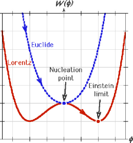
FIG. 1.: Geodetic brane nucleation: From the Euclidean no-boundary initial conditions to the Einstein limit.

The smoothness of the Euclidean manifold at the origin dictates the specific $\tau\rightarrow 0$ behavior $a_{E}(\tau)\simeq\sqrt{k}\tau$, but may in principle allow for $\displaystyle{b_{E}(\tau)\simeq\frac{p\sqrt{k}}{\tau^{j-1}}}$. Now, assuming the asymptotic power behavior

$$W(\phi)\simeq\lambda\phi^{N}\quad(\lambda>0)~{},$$ (30)

the scalar equation of motion eq.(28) can be fulfilled (to the leading order) only provided

$$jN=2(j+1)~{},\quad N\lambda p^{(N-2)}+j(j-2)=0~{}.$$ (31)

This in turn implies $\rho\sim\tau^{-2(j+1)}$ but $\rho_{total}\sim\tau^{4(j-1)}$. Consequently, fully consistent with our expectations, $N$ gets uniquely fixed by insisting on approaching a finite non-vanishing total energy density limit as $a_{E}\rightarrow 0$. This singles out $j=1\Rightarrow N=4$. The generalized no-boundary initial conditions then read

$$a_{E}\simeq\sqrt{k}\tau~{},\quad b_{E}\simeq\frac{k}{4\lambda}~{},$$ (32)

accompanied by the finite total energy density

ρtotal≃(4ωλ3k2)2 (33)

While the no-boundary initial conditions are in fact $\omega$-independent, it is $\omega$ which fixes the finite total energy density. It is interesting to note that had we carried out a similar calculation for an $n$-brane (we skip the proof due to length limitation), we would have encountered the famous scale invariant behavior

$$W(\phi)\sim\phi^{\frac{2(n+1)}{n-1}}~{},$$ (34)

which happens to be quartic if $n=3$. This indicates that, within the framework of geodetic brane cosmology, there exists a linkage between (the apparently disconnected ideas of) Hawking-Hartle no-boundary proposal and global conformal invariance, pointing presumably towards geodetic dilaton cosmology.

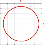
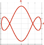
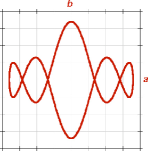
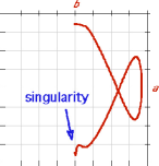
FIG. 2.: Imaginary time periodicity and energy density regularity are demonstrated, for $\omega_{1,3,5}$, by means of closed trajectories in the $\{a_{E},b_{E}\}$ plane. If $\omega\neq\omega_{n}$, a $\cos(\ln\epsilon)$-type singularity is developed upon returning to the origin.

Finally, on realistic grounds, while adopting the quartic Higgs potential, it makes sense to exercise the option of setting $W_{min}(\phi)$ to zero. The price for eliminating the residual cosmological constant from the Einstein limit is a finite (yet enhanced in comparison with standard cosmology) amount of inflation. Subject to the consistent no-boundary initial conditions eq.(32), the classical Euclidean evolution is fully determined once the conserved bulk energy $\omega$ gets specified. Naturally, this provokes a new set of questions: (i) Does the global structure of the Euclidean manifold still exhibit imaginary time periodicity? (ii) Under what circumstances, if any, does the total energy density evolve free of singularity? (iii) Can our nucleation conditions $a_{E}^{\prime}=\phi_{E}=0$, or else Coleman-Dellucia[10] conditions $a_{E}^{\prime}=\phi_{E}^{\prime}=0$, be met at some finite Euclidean time $\tau_{0}$?

We claim, skipping the analytic proof (to be published elsewhere) due to length limitation, that $\tau$-periodicity, $a_{E},b_{E}$-regularity, and spontaneous nucleation, share the one and the same origin. They can all be simultaneously achieved provided $\omega=\omega_{n}$ is properly quantized, in agreement with some previous WKB approximation[6]. The integer $n$ counts the total number of times the proper scalar field $b_{E}$ crosses the absolute minimum of the potential during half a period. For the $n$-odd case of interest ($n$-even is associated with Coleman-Dellucia), reflecting the interplay of two periodicities, we encounter (see Fig. 2) $n$-loop closed trajectories in the $\{a_{E},b_{E}\}$ plane which resemble the Lissajous figures. Notice that the Euclidean de-Sitter configuration eq.(27) clearly belongs to the $n=1$ category.

REFERENCES

- [1] L. Randall and R. Sudrum, Phys. Rev. Lett. 83, 3370 (1999).
- [2] T. Regge and C. Teitelboim, in Proc. Marcel Grossman (Trieste), 77 (1975).
- [3] E. Kasner, Am. Jour. Math. 43, 126, 130 (1921); C. Fronsdal, Phys. Rev. 116, 778 (1959) Y. Ne’eman and J. Rosen, Ann. of Phys. 31, 391 (1965); J. Rosen, Rev. Mod. Phys. 37,204 (1965); H.F. Goenner, in General Relativity and Gravitation (ed. A. Held, Plenum), 441 (1980); S. Deser and O. Levin, Phy. Rev. D59, 064004 (1999).
- [4] G.W. Gibbons and D.L. Wiltshire, Nucl. Phys. B287, 717 (1987); R. Basu, A.H. Guth and A. Vilenkin, Phys. Rev. D44, 340 (1991).
- [5] S. Deser, F.A.E. Pirani, and D.C. Robinson, Phys. Rev. D14, 3301 (1976). V. Tapia, Class. Quan. Grav. 6, L49 (1989); M. Pavsic, Phys. Lett. A107, 66 (1985); D. Maia, Class. Quan. Grav. 6, 173 (1989); I.A. Bandos, Mod. Phys. Lett. A12, 799 (1997).
- [6] A. Davidson, Class. Quan. Grav. 16, 653 (1999); A. Davidson, D. Karasik, and Y. Lederer, Class. Quant. Grav. 16, 1349 (1999).
- [7] S. Coleman and K. Lee, Nucl. Phys. B329, 387 (1990).
- [8] J.B. Hartle and S.W. Hawking, Phys. Rev. D28,2960 (1983); J.J. Halliwell and S.W. Hawking, Phys. Rev. D31, 1777 (1985).
- [9] S.W. Hawking and I.G. Moss, Phys. Lett. 110B, 35 (1982); A.D. Linde, Sov. Phys. JETP 60, 211 (1984); A. Vilenkin, Phys. Lett. 117B, 25 (1982); A. Vilenkin, Phys. Rev. D30, 509 (1984); N. Turok and S.W. Hawking, Phys. Lett. B425, 25 (1998); A.D. Linde, Phys. Rev. D58, 083514 (1998) ; A. Vilenkin, Phys. Rev. D57, 7069 (1998).
- [10] S. Coleman and F. De Luccia, Phys. Rev. D21, 3305 (1980).