Abstract

We study the addition of an irrelevant operator to the ${\cal N}=4$ supersymmetric large $N$ $SU(N)$ gauge theory, in the presence of finite temperature, $T$. In the supergravity dual, the effect of the operator is known to correspond to a deformation of the AdS${}_{5}\times S^{5}$ “throat” which restores the asymptotic ten dimensional Minkowski region of spacetime, completing the full D3–brane solution. The system at non–zero $T$ is interesting, since at the extremes of some of the geometrical parameters the geometry interpolates between a seven dimensional spherical Minkowskian Schwarzschild black hole (times ³) and a five dimensional flat AdS Schwarzschild black hole (times $S^{5}$). We observe that when the coupling of the operator reaches a critical value, the deconfined phase, which is represented by the geometry with horizon, disappears for all temperatures, returning the system to a confined phase which is represented by the thermalised extremal geometry.

1 Introduction

A number of important spacetime solutions of general relativity and string theory have the interesting feature that they have an infinite “throat” spacetime at their core, connected to the asymptotically flat region by an interpolating region or “mouth”. A simple prototype of this is the extremal Reissner–Nordstrom black hole in four dimensions, at whose core there is AdS${}_{2}\times S^{2}$, the Bertotti–Robinson universe[1]. This behaviour persists to various spacetime solutions of string and M–theory, such as magnetically charged black holes[2, 3, 4], various branes[5] such as three–branes[6] and M–branes[7], and heterotic or symmetric five–branes[8, 9].

The throat regions, usually possessing a high degree of symmetry, have been of some considerable interest in string theory, since they are often realisable as exact solutions, and some even have representations as interesting conformal field theories (CFT’s). For example, a two dimensional black hole can be written as an exact CFT[10], using a gauged Wess–Zumino–Novikov–Witten (WZNW) model. By tensoring this with other CFT’s or embedding it into larger gauged WZNW models to obtain non–trivial mixing between the radial and angular sectors, this sort of model forms part of the exact CFT description of the throat limit of various higher dimensional objects (e.g., fivebranes[11], four dimensional magnetic holes[12], four dimensional dyonic and/or rotating holes and Taub–NUT spacetimes, etc[13].) Throats are hence important examples of how non–trivial backgrounds are represented in string theory. See figure 1.

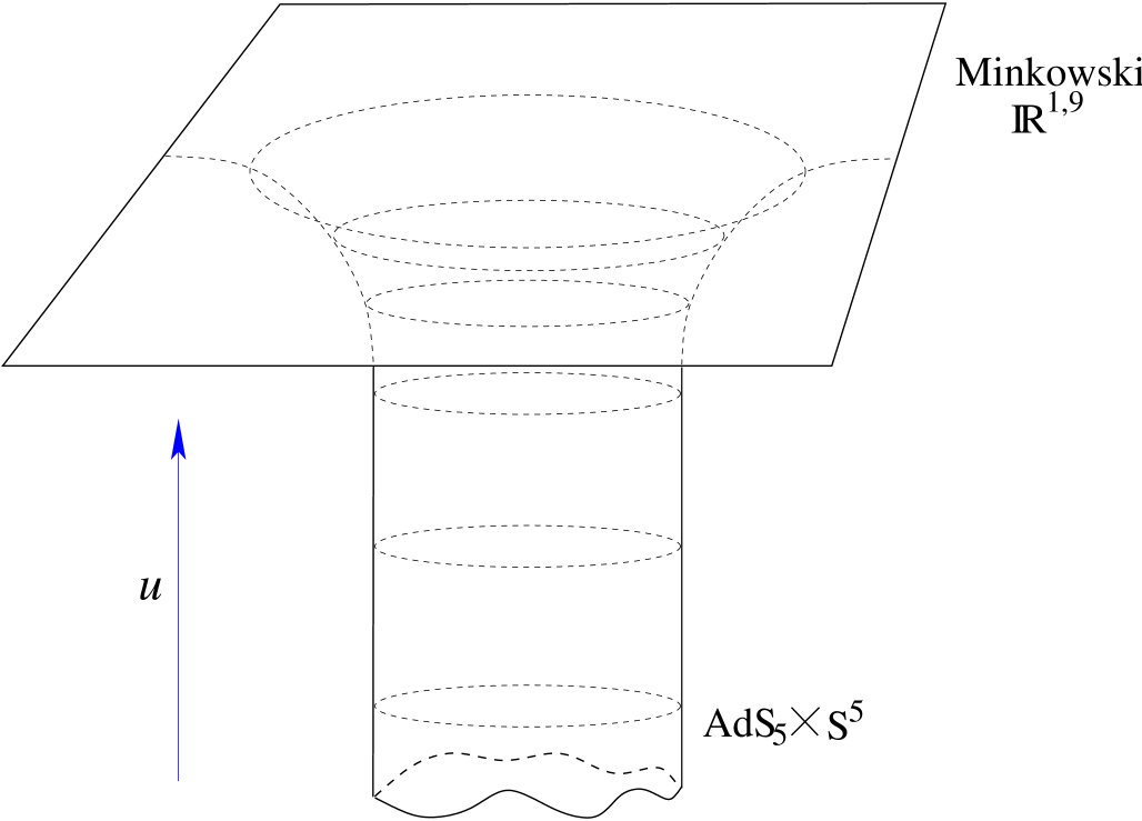
Figure 1: The generic “throat$+$mouth” geometry of some string backgrounds of interest. We have labelled it as appropriate to the three–brane case, for later discussion.

A significant step in the direction of maturity of this approach was made when the AdS${}_{5}\times S^{5}$ throat at the core of the geometry of $N$ coincident D3–branes[6] was identified[14, 15, 16] as being a dual description of ${\cal N}=4$ supersymmetric $SU(N)$ gauge theory at large $N$. This particular model makes concrete many highly non–trivial ideas about how a theory of quantum gravity operates (such as holography[17], UV/IR relations[18]), provides us with new tools for testing ideas about strongly coupled gauge theories, and may even be thought of as the best understood (at least in principle) non–perturbative definition of a ten dimensional superstring theory.

One technical feature of interest in representing these throat geometries in string theory has been the issue of how to describe —directly within the field theory representation itself— the process of moving out of the throat back to the asymptotic region. This was once of great interest since it was hoped (for example) that one might be able to represent in this way the $S$–matrix for the scattering of quanta off a black hole, in a bid to solve the black hole information puzzle.

In this note we study the AdS${}_{5}\times S^{5}$ throat geometry, and its connection to the asymptotically flat region to make the complete D3–brane geometry. The AdS/CFT Correspondence identifies each supergravity field with an operator in the dual gauge theory and so switching on these extra metric components should correspond to some deformation of the field theory. Restoring the throat region relaxes the decoupling limit of the AdS/CFT Correspondence and hence would be expected to introduce gravitational and stringy couplings back into the field theory. We expect these effects to show up in the form of higher dimension operators. In refs.[19, 20] (see also e.g., [21]) the connection to the asymptotically flat region of the D3–brane geometry was identified as the addition of an irrelevant operator of the form ${\rm Tr}F^{4}$, which does not destroy the conformal nature of the gauge coupling. Alternatively, in [22] the asymptotically flat region was recovered in a low energy limit of a multi-centre D3 brane geometry describing a point on the moduli space of the ${\cal N}=4$ gauge theory. Here the operator encodes the scalar vevs at a large scale above which the gauge symmetry is enlarged. There are clearly many UV completions of the theory which in the IR give rise to a higher dimension operator of this form. Here we wish to study the role of the operator on the system without specifying the UV completion in the spirit of, for example, the Nambu-Jona-Lasinio (NJL) model [23]. We will make comparisons to the NJL model in the final discussion. In particular we study the role of this higher dimension operator on the finite temperature behaviour of this system. The geometry is interesting, since the non–extremal D3–brane geometry contains richer features than the extremal case.

One of the most interesting of such features is that at the core there is the $D=5$ (flat) AdS–Schwarzschild black hole (times $S^{5}$), while asymptotically the geometry has a limit which is a $D=7$ asymptotically Minkowskian (spherical) Schwarzschild black hole (times ³). The relevance of the former to the dual gauge theory has already been demonstrated in ref.[24] as representing the deconfined finite temperature phase. The presence of the irrelevant operator should therefore imply a possible role for the asymptotically flat $D=7$ black hole in the thermodynamics of the deformed gauge theory. We allow for this possibility here.

In order to make sense of these spacetimes in terms of the dual gauge dynamics it is important to realise that a non–renormalisable operator implicitly implies the existence of a cut–off, $\Lambda$, in the UV. Usually such operators indicate the presence of new physics above $\Lambda$. We represent this in the geometries (as we would expect from the usual UV/IR relation) by an IR cut–off on the size of the space, taking the usual radial parameter out to a finite value, $u_{\rm max}$. When $\Lambda$ (i.e., $u_{\rm max}$) is sufficiently small that it lies in the AdS part of the space, the physics is simply that of the usual AdS/CFT correspondence. The AdS black holes, which have a temperature proportional to their radius, are energetically preferred over a thermalised version of AdS[24].

In the opposite extreme where $\Lambda$ is taken large, and so the full asymptotically flat geometry is available, we must also consider the geometry which includes the Minkowskian black holes whose temperature is inversely proportional to their radius. Since the AdS and the Minkowskian black holes mutate into each other it is clear that there is a maximum temperature black hole geometry. At temperatures above this maximum value the thermalised extremal solution with no horizon (representing the confined phase) is the only possible geometry. A computation of the free energies of the non–extremal solution (which contains both types of black hole as limits) and the thermalised extremal solution below this temperature reveals the stronger result that the black hole solutions are never favoured. This shows that the non–renormalisable operator destroys the deconfined phase, favouring the confined phase. When $\Lambda$ is taken large the non–renormalisable operator’s coupling is large and the cut–off physics dominates. A temperature below the $\Lambda$ can then not change the phase of the theory.

As the cut–off $\Lambda$ is reduced, making the available space more AdS–like, the non–renormalisable operator’s coupling falls (or since there is only one scale in the problem we may view this as changing the coupling at fixed $\Lambda$). At a critical value for the coupling the behaviour switches between the two limits with AdS black holes becoming the favoured high temperature phase. Below this value the coupling at the cut–off is sufficiently small so as to be irrelevant to the IR dynamics.

Note that when $\Lambda$ is taken large, the Minkowski black holes, whose radii are very close to the cut–off have a very negative free energy. Naively therefore, they appear to be the dominant low temperature phase at high cut–off, but we discard this possibility for two reasons. The first is that their large size is comparable to $\Lambda$ (i.e., $u_{\rm max}$), suggesting that in the field theory such states can not be considered without including corrections from trans–cut–off physics. The other is that they have negative specific heat and hence cannot represent a stable (in the canonical ensemble we consider here) dual field theory vacuum. We expect that further work will find a role for them in the non–equilibrium dynamics of the perturbed theory, but this is not addressed in this paper.

The structure of this short note is as follows: In the next section, we present a reminder of the properties of the non–extremal D3–brane solution, and a brief orientation on matters concerning the throat limits and their relation to the dual field theory. Section 3 introduces the irrelevant operator, the return to flat space, and reports on the Euclidean action computation which we perform. We uncover the phase structure, and draw a phase diagram in figure 5, summarising the role of how the operator and the cut–off work together in this beyond–AdS/CFT exploration. We end with a brief recapitulation and discussion in the final section.

2 The Geometry of D3–branes

The fields[6]:

$$ds^{2} = Z_{3}^{-{1\over 2}}(r)\left(-K(r)dt^{2}+dx_{1}^{2}+dx_{2}^{2}+dx_{3}^{2}\right)+Z_{3}^{1\over 2}(r)\left(K(r)^{-1}dr^{2}+r^{2}d\Omega_{5}^{2}\right),\$$

$$C_{(4)} = \alpha_{3}^{-1}Z_{3}^{-1}dt\wedge dx_{1}\wedge dx_{2}\wedge dx_{3},\$$ (1)

with

$$Z_{3} = 1+\alpha_{3}\frac{r_{3}^{4}}{r^{4}}\ ,\qquad K=1-\frac{r_{H}^{4}}{r^{4}}\ ,$$

$$r_{3}^{4} = 4\pi g_{s}N\alpha^{\prime 2}\ ,\qquad\alpha_{3}=\sqrt{1+\left(\frac{r_{H}^{4}}{2r_{3}^{4}}\right)^{2}}-\frac{r_{H}^{4}}{2r_{3}^{4}}$$

solve the following truncation of the ten dimensional type IIB supergravity equations of motion:

$$R^{\mu}_{\phantom{\mu}\nu}+{1\over 240}T^{\mu}_{\phantom{\mu}\nu}=0\ ,$$ (2)

where

$$T^{\mu}_{\phantom{\mu}\nu}=5G_{(5)}^{\mu\alpha\beta\gamma\delta}G_{(5)\nu\alpha\beta\gamma\delta}-\frac{1}{2}\delta^{\mu}_{\phantom{\mu}\nu}G_{(5)}^{2}\ ,\qquad\mbox{and}\quad G_{(5)}=dC_{(4)},$$ (3)

which can be derived from the action:

$$I=\frac{1}{2\kappa^{2}}\int d^{10}\!x\sqrt{-G}\left(R-\frac{1}{240}G_{(5)}^{2}\right)\ .$$ (4)

Newton’s constant is set by $2\kappa^{2}\equiv 16\pi G_{N}=(2\pi)^{7}\alpha^{\prime 4}g_{s}^{2}$ where $g_{s}$ is the dimensionless closed string coupling and $\alpha^{\prime}$, with dimensions of a squared length, sets the inverse string tension. The solution has $N$ units of D3–brane charge, $\mu_{3}=(2\pi)^{-3}(\alpha^{\prime})^{-2}$.

2.1 The Extremal Limit and the Throat

In the limit $r_{H}\to 0$, we find that $\alpha_{3}\to 1$, and we recover the extremal solution preserving 16 supercharges, representing $N$ coincident BPS D3–branes lying in the $x_{1},x_{2},x_{3}$ directions. Their low energy dynamics, $\alpha\to 0$, are captured[26] by the $SU(N)$ gauge theory manifest in their open string description which is useful when $g_{s}N<1$. The gauge coupling is given by $g^{2}_{\rm YM}=2\pi g_{s}$. As is well known, the limit $g_{s}N>1$ has a good description in terms of the closed string fields. Writing $r_{3}=\sqrt{\alpha^{\prime}}\ell$ and $r=\alpha^{\prime}u$, defining a characteristic energy scale $u$ in the gauge theory, the closed string fields describe the smooth supergravity geometry at the “throat”:

$$\frac{ds^{2}}{\alpha^{\prime}}=\frac{u^{2}}{\ell^{2}}\left(-dt^{2}+dx_{1}^{2}+dx_{2}^{2}+dx_{3}^{2}\right)+{\ell^{2}}\frac{du^{2}}{u^{2}}+\ell^{2}d\Omega_{5}^{2}\ ,$$ (5)

which is AdS${}_{5}\times S^{5}$ with characteristic length scale $L=\ell\sqrt{\alpha^{\prime}}$. The radial parameter $u$ transforms with unit mass dimension in the dual field theory[14, 15, 16], as appropriate for an energy scale. The scaled harmonic function which appears implicitly in the above geometry $H={\ell^{4}}/{u^{4}}$, controlling the standard D3–brane form $(\alpha^{\prime})^{-1}ds^{2}\sim H^{-{1\over 2}}dx_{\parallel}^{2}+H^{{1\over 2}}dx_{\perp}$ can be extended to encode the insertion of ${\cal N}=4$ preserving scalar operators in the dual gauge theory[27]. For example, the form:

$$H=\frac{\ell^{4}}{u^{4}}\left(1+\frac{c_{ij}Y^{ij}}{u^{2}}+\cdots\right)$$ (6)

encodes the insertion of the dimension $\Delta=2$ operator ${\cal O}_{ij}\sim{\rm Tr}[\Phi_{(i}\Phi_{j)}]$, with vacuum expectation value $c_{ij}$, which is in the ${\bf 20^{\prime}}$ of the $SO(6)\simeq SU(4)$ R–symmetry, made of the symmetric product of the six adjoint scalars $\Phi_{i}$, $i=1,..,6$, in the gauge multiplet. The $Y^{ij}(\theta,\phi,\ldots)$ schematically represent the $S^{5}$ spherical harmonics in the ${\bf 20^{\prime}}$. The limit of large $u$ is the UV in the gauge theory, and we see that the operator becomes increasingly small, as appropriate for a relevant deformation.

2.2 Non–Extremality and Finite Temperature

There are two natural candidate geometries which we might study as representing the gravity dual of the gauge theory at finite temperature[24]. One is AdS${}_{5}\times S^{5}$ itself, now filled with quantum fields at temperature $T$, and the other is the AdS₅ black hole (times $S^{5}$) with a flat horizon. They are both candidates since they are asymptotically AdS${}_{5}\times S^{5}$, which is appropriate since temperature may be represented as a relevant operator in a low energy effective action. The black hole solution may be obtained by taking the same throat limit as before, but of the non–extreme solution given in equation (1), to give:

$$\frac{ds^{2}}{\alpha^{\prime}}=-\left(\frac{u^{2}}{\ell^{2}}-\frac{u_{H}^{4}}{\ell^{2}u^{2}}\right)dt^{2}+\frac{u^{2}}{\ell^{2}}\left(dx_{1}^{2}+dx_{2}^{2}+dx_{3}^{2}\right)+\left(\frac{u^{2}}{\ell^{2}}-\frac{u_{H}^{4}}{\ell^{2}u^{2}}\right)^{-1}{du^{2}}+\ell^{2}d\Omega_{5}^{2}\ ,$$ (7)

where now $\ell^{2}=\alpha_{3}^{1\over 2}r_{3}^{2}/\alpha^{\prime}$, and $u_{H}=r_{H}/\alpha^{\prime}$. The temperature of this solution is naturally determined by requiring regularity of the Euclidean section, with the result[28]

$$T\equiv\beta^{-1}=\frac{u_{H}}{\pi\ell^{2}}\ ,$$ (8)

and this must be compared to AdS${}_{5}\times S^{5}$ thermalised at the same temperature (defined for example by compactifying the Euclidean time coordinate[28]).

We must let the thermodynamics choose between the two solutions. We can define for this system a canonical thermodynamic ensemble at finite temperature $T$ by continuing the action $I$ in the path integral $Z$ to a Euclidean one ${\hat{I}}=-iI$, via $t\to-i\tau$, defining a partition function using a periodicity, $\beta$, of $\tau$

$$Z=\int{\cal D}[G]\exp{(-{\hat{I}})}=\sum_{n}\exp{(-\beta E_{n})}\ .$$ (9)

A careful computation in the semiclassical approximation reveals that the free energy $F=W={\hat{I}}/\beta$ of AdS₅–Schwarzschild is lower than that of AdS₅ for all $\beta$, (see figure 2), showing that it is favoured as the geometry representing the finite temperature phase[24] which is deconfined. This computation is the low cut–off limit of the more general calculation we present in the next section.

Figure 2: The thermodynamic potential $W$, or free energy $F$ of the AdS₅ black holes (relative to AdS₅) as a function of temperature $T$. It is negative for all $T$, showing that these black holes dominate the thermodynamics, forming the deconfined phase for all $T$.

3 An Irrelevant Operator

Consider modifying the harmonic function $H$ as follows:

$$H=\frac{\ell^{4}}{u^{4}}\left(\mbox{g}u^{4}+1+\cdots\right)\ ,$$ (10)

and we will ignore all other operators in the discussion that follows. The coupling ${\rm g}$ (with mass dimension of ${-4}$) couples to a new operator, ${\cal O}$, which therefore has a mass dimension of ${8}$, and has no R–charge. As discussed in the introduction a number of UV completions of this higher dimension operator can be envisaged. In [19, 20] the operator was identified with ${\rm Tr}F^{4}$ or $({\rm Tr}F^{2})^{2}$, or a mixture of the two. In [22] it was shown that the geometry could be embedded as a limit of a multi-centre D3 geometry and in that case the operator represents scalar vevs at some high scale. If the geometry is taken in isolation, without embedding in a multi-centre solution, then supergravity is not decoupled completely from the theory, almost by definition: we are connecting the throat, and hence the branes, back to the asymptotic regime where they can communicate by exchanging gravitons, etc, with the outside world. Gravitational effects may therefore also contribute to the higher dimension operator. So we have in mind that this single operator represents the leading effect of having integrated out the physics of the full theory in the UV but will not specify that theory explicitly in the analysis to follow.

The existence of the non–renormalisable operator in the field theory invites us to include a UV cut–off, $\Lambda$, at which new physics responsible for the operator is present. A UV cut–off in the field theory corresponds to an IR cut–off, $u_{\rm max}$, on the radius of the geometry. We may also think of changing the cut–off as equivalent to changing the coupling ${\rm g}$ at a fixed $\Lambda$ since there is only one new scale in the theory. We can see that as we raise $\Lambda$ the operator’s effects grow, with the space including more of the asymptotic Minkowski geometry, consistent with the operator becoming more strongly coupled.

Geometrically, the deformation corresponds to adding the part of the harmonic function which connects AdS${}_{5}\times S^{5}$ to asymptotically flat spacetime, allowing us to move “clear” of the throat region. In the field theory a mass scale has been introduced corresponding to (roughly) the radial distance at which the two geometries interchange. This is natural from the point of view of the full solution given in equation (1), and the coupling can be seen to scale as ${\rm g}\sim(\alpha^{\prime})^{2}$. This term usually vanishes in the decoupling limit of the AdS/CFT correspondence, and adding this operator is equivalent to restoring it. This is highly appropriate, since adding a higher dimension operator requires the introduction of a new dimensionful scale in the theory, which represents the physics which has been integrated out in forming this effective operator. Morally, we know what physics has been integrated out: it is the full type IIB string theory in the presence of three–branes.

Now that we have relaxed the $\alpha^{\prime}\to 0$ limit, we ought to worry about stringy corrections in $\alpha^{\prime}$ completely invalidating our discussion of the supergravity solution. However, we will still keep $\alpha^{\prime}$ small, and also restrict ourselves to the limit of strong ’t Hooft coupling $g_{\rm YM}^{2}N$ so as to keep all higher derivative corrections (coming from curvature) under control.

The supergravity solution is obtained by simply taking the solution of equation (1), in the extremal limit $r_{H}=0$, $\alpha_{3}=1$, and writing it in terms of $u$ (recall that $\ell^{2}=r_{3}^{2}/\alpha^{\prime}$):

$$\frac{ds^{2}}{\alpha^{\prime}}=\left(\alpha^{\prime 2}+\frac{\ell^{4}}{u^{4}}\right)^{-{1\over 2}}\left(-dt^{2}+dx_{1}^{2}+dx_{2}^{2}+dx_{3}^{2}\right)+\left(\alpha^{\prime 2}+\frac{\ell^{4}}{u^{4}}\right)^{{1\over 2}}\left(du^{2}+u^{2}d\Omega_{5}^{2}\right)$$ (11)

In the limit $\alpha^{\prime}\to 0$, the operator vanishes and we return to the throat solution of equation (5).

3.1 Going to Finite Temperature

We are interested in learning more about the role of the operator in the theory by studying it at finite temperature. Now as before, there are at least two candidate geometries for what might represent the appropriate dual geometry at temperature $T$. One is the asymptotically flat geometry, but thermalised, while the other is a geometry with an horizon, which we write in the gauge theory variables, starting from the brane solution in equations (1) again:

$$\frac{ds^{2}}{\alpha^{\prime}} = \bar{Z}_{3}(u)^{-{1\over 2}}\left(-\bar{K}(u)dt^{2}+dx_{1}^{2}+dx_{2}^{2}+dx_{3}^{2}\right)+\bar{Z}_{3}(u)^{{1\over 2}}\left(\bar{K}(u)^{-1}du^{2}+u^{2}d\Omega_{5}^{2}\right)$$ (12)

$${C_{(4)}\over\alpha^{\prime 2}} = \alpha_{3}^{-1}\bar{Z}_{3}(u)^{-1}dt\wedge dx^{1}\wedge dx^{2}\wedge dx^{3}$$ (13)

where

$$\bar{Z}_{3}(u)=\left(\alpha^{\prime 2}+\frac{\ell^{4}}{u^{4}}\right),\hskip 28.45274pt\bar{K}(u)=\left(1-\frac{u_{H}^{4}}{u^{4}}\right)\ ,$$ (14)

and now $\ell^{2}=\alpha_{3}^{1\over 2}r_{3}^{2}/\alpha^{\prime}$. This geometry naturally has a temperature given by

$$\beta=\pi r_{H}\left[\frac{1}{2}+\sqrt{\left(\frac{{r}_{3}^{4}}{r_{H}^{4}}\right)^{2}+\frac{1}{4}}\right]^{1\over 2}=\pi u_{H}\left[\frac{\alpha^{\prime 2}}{2}+\sqrt{\left(\frac{\ell^{4}}{u_{H}^{4}}\right)^{2}+\frac{\alpha^{\prime 4}}{4}}\right]^{1\over 2}\ ,$$ (15)

obtained by the usual requirement of Euclidean regularity. Notice that it returns to the expression (8) for the AdS₅–Schwarzschild black hole when we switch off the operator by sending $\alpha^{\prime}\to 0$. We have plotted it as a function of $r_{H}$ in the case of non–zero $\alpha^{\prime}$ for later use, in figure 3. In fact there are two classes of solutions for each temperature, a small and large branch. The smaller solutions are the ones which become the AdS₅ black holes. From the slope of the curve, they have positive specific heat, while the larger ones, which more closely resemble $D=7$ Schwarzschild black holes, have negative specific heat, showing that they are unstable.

Figure 3: The temperature of the non–extremal D3–brane solution as a function of $r_{H}$. Note two features: (1) There are two available solutions for each temperature, the smaller have positive specific heat and the larger have negative specific heat. (2) There is a maximum temperature beyond which there are no solutions.

At low temperatures, for the larger branch, we see that $r_{H}$ (or $u_{H}$) increases and in the limit of it being large, we see from equation (1) that $\alpha_{3}\to 0$, $\ell\to 0$, and the geometry becomes:

$$ds^{2} = -\left(1-\frac{r_{H}^{4}}{r^{4}}\right)dt^{2}+dx_{1}^{2}+dx_{2}^{2}+dx_{3}^{2}+\left(1-\frac{r_{H}^{4}}{r^{4}}\right)^{-1}dr^{2}+r^{2}d\Omega_{5}^{2}\ ,$$ (16)

which is simply the round asymptotically flat $D=7$ Schwarzschild solution multiplied by ³. It would be intriguing if there was a role for this object in the context of a dual four dimensional gauge theory (deformed by an operator), and we shall see shortly how it fits into the story.

3.2 Thermodynamic Choices

To find out which geometry is appropriate at finite temperature $T$, we should compare the relative free energies of the two geometries. This is an amusing computation, and it is worth describing it here. We compute the action by continuing to Euclidean space, and writing:

$${\hat{I}}=-\frac{1}{2\kappa^{2}}\int_{\cal M}d^{10}\!x\sqrt{-G}\left(R-\frac{1}{480}G_{(5)}^{2}\right)-\frac{1}{\kappa^{2}}\int_{\partial{\cal M}}d^{9}\!x\sqrt{-h}\,{\cal K}\ .$$ (17)

where ${\cal M}$ is spacetime, ${\cal K}$ is the trace of the extrinsic curvature tensor defined on the boundary $\partial{\cal M}$, which here will be at our cut–off radius, and $h_{\mu\nu}$ is the nine–dimensional boundary metric.

In fact, the computation is simplified considerably by the property of both of our solutions, the vanishing of the Ricci scalar $R$. The $G_{(5)}$ action term may be easily evaluated:

$$\frac{1}{\kappa^{2}}\int_{\cal M}d^{10}\!x\sqrt{-G}\frac{1}{480}G_{(5)}^{2} = {\alpha^{\prime 4}\over 4\kappa^{2}}{\rm Vol}(S^{5})V_{3}{\beta\over\alpha_{3}^{2}}\int_{u_{H}}^{u}{x^{5}\over\bar{Z}_{3}(x)^{2}}\bar{Z}_{3}^{\prime}(x)^{2}dx$$ (18)

$$= -{{\rm Vol}(S_{5})V_{3}\beta\over 2\kappa^{2}}\frac{l^{8}}{\alpha_{3}^{2}}\left[{\alpha^{\prime 2}\over x^{4}\alpha^{\prime 2}+\ell^{4}}\right]_{u_{H}}^{u}$$

where ${\rm Vol}(S^{5})$ is the volume of the $S^{5}$ and $V_{3}$ is the volume of the ³ along the brane.

Some algebra yields the following result for the trace of extrinsic curvature of the general solution:

$${\cal K}(u)=\frac{1}{2\sqrt{G_{uu}}}G^{\mu\nu}\frac{\partial G_{\mu\nu}}{\partial u}={1\over 2\alpha^{\prime 1/2}}\frac{\bar{K}^{1/2}}{\bar{Z}_{3}^{1/4}}\left[\frac{\bar{K}^{\prime}}{\bar{K}}+{1\over 2}\frac{\bar{Z}_{3}^{\prime}}{\bar{Z}_{3}}+\frac{10}{u}\right]\ ,$$ (19)

and we also have

$$\sqrt{-h}=\alpha^{\prime 9/2}u^{5}\bar{Z}_{3}^{1/4}(u)\bar{K}^{1/2}(u)\varepsilon_{5}\ ,$$ (20)

where $\varepsilon_{5}$ is the square root of the determinant of the metric of a round $S^{5}$ of unit radius. The final term in ${\cal K}$ will produce a severe divergence in the large $u$ limit, but happily the divergence cancels in the difference between the action of the non–extremal and the extremal solution, and so we shall avoid it.

Now the rest is straightforward, except for one important subtlety: While the result for the integral over $\tau$ for the non–extremal solution is simply $\beta$, given in equation (15), this should not be used as the time period in performing the integral over the extremal solution, if we are to compare the two accurately. Recall that the periodicity of the time coordinate of a solution sets the inverse temperature. However, at radius $r$, there are redshift factors which change the temperature, coming from the fact that the geometry is curved. If we use $\beta$ for the non–extremal geometry, we should use $\beta^{*}$ for the extremal geometry, where

$$\beta^{*}=\beta\,\bar{Z}_{3}^{-1/4}(u)\bar{K}^{1/2}(u)\bar{Z}_{3}^{1/4}(u,\alpha_{3}=1)\ .$$ (21)

So we can now put this all together to compute the following expression for the action difference at radius $u$:

$${\hat{I}} = -\frac{V_{3}}{\kappa^{2}}{\rm Vol}(S^{5})\Biggl{[}\beta\left\{\sqrt{-h}\,{\cal K}(u)+{\ell^{8}\alpha^{\prime 2}\over 2\alpha_{3}^{2}}\left({1\over\alpha^{\prime 2}u^{4}+\ell^{4}}-{1\over\alpha^{\prime 2}u_{h}^{4}+\ell^{4}}\right)\right\}$$ (22)

$$\hskip 56.9055pt-\beta^{*}\left\{\sqrt{-h}\,{\cal K}(u)+{\ell^{8}\alpha^{\prime 2}\over 2\alpha_{3}^{2}}\left({1\over\alpha^{\prime 2}u^{4}+\ell^{4}}-{1\over\ell^{4}}\right)\right\}_{\alpha_{3}=1\atop u_{H}=0}\Biggr{]}\ ,$$

where it is to be understood that all of the terms in the braces in the last line are to be evaluated at $\alpha_{3}=1$, $u_{H}=0$, since they refer to the contribution of the extremal solution.

Since this is a rather clumsy expression, we plot it numerically in figure 4 for varying cut–off, $u_{\rm max}$, in order to see the result. When the cut–off is small so the space is essentially AdS the AdS black holes are thermodynamically favoured over the thermalised extremal solution at finite temperature. The surface term is small (vanishing in the pure AdS limit) and the physics is dominated by the gauge field strength term which is negative. There is therefore a transition from a confined phase at $T=0$ to a deconfined phase at finite $T$.

Figure 4: The thermodynamic potential $W$, or free energy $F$ (relative to the extremal solution) as a function of temperature $T$. (a) The free energy for different values of the cutoff below and above the critical cut–off. When the cut–off is low (bottom curve) the behaviour is like the pure AdS₅ case (see figure 2) with a deconfined phase while with a large cut–off (top curve) the confined phase is always preferred. (b) Large cut–off $\Lambda$: the snout shape is made of two branches, the steep part coming over the top corresponds to the large $D=7$ black holes, and the other branch to the smaller holes, which form the AdS₅ black holes in the throat limit. (At a certain temperature both branches merge and extend no further to the right.) With the large cut–off none of these black holes are favoured: We ignore the appearance of a negative free energy for the $D=7$ holes for low enough temperature, since they are unstable. Furthermore, at low enough temperatures they are simply too large for the cut–off.

As the cut–off is raised the positive surface term grows until at a critical value it dominates the field strength term and the free energy difference becomes positive. Above this critical cut–off the thermalised extremal solution representing the confined phase is energetically preferred. This fits our field theory intuition; as the cut–off $\Lambda$ is raised, the non–renormalisable operator becomes more strongly coupled at the cut–off and at some critical value we would expect the dynamics to be controlled by that coupling at the cut–off. Then a temperature below $\Lambda$ will not influence the dynamics. It is interesting that the operator forces the theory back to the confined phase.

Finally we note that when we take $\Lambda$ very large so that Minkowskian Schwarzschild black holes are possible, their relative free energy falls rapidly negative with decreasing $T$ and their radius approaches the cut off scale. It would be nice to associate a resulting role at low temperature for these $D=7$ holes. However, it should be remembered that these holes have negative specific heat and so are unstable in this canonical ensemble (they may simply radiate away), and in any case their size is sufficiently close to the cut–off that in the field theory such states must presumably know about trans–cut–off physics which is unspecified. Without detailed knowledge of what lies outside the cut–off we can not truly evaluate their role.

We display the phase diagram as a function of $T$ and the dimensionless coupling of the higher dimension operator graphically in figure 5.

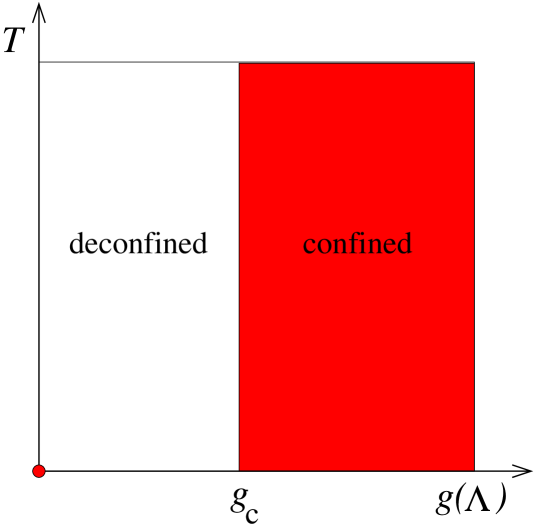
Figure 5: The phase diagram of the field theory as a function of $T$ and the coupling of the higher dimension operator. The origin is in the confined phase. There is a critical value of the cutoff $\Lambda$ or the operator’s coupling ${\rm g}$ at which there is a phase transition back to the confined phase.

4 Discussion

We have learned some interesting information about how to describe the rest of the D3–brane supergravity geometry in the context of the large $N$ conformal gauge theory that is dual to the theory living at the AdS${}_{5}\times S^{5}$ throat. This is quite promising, since getting dual descriptions of the region beyond a throat (while still using the field theory description often afforded by the throat limit) has proven to be an arduous task in the past.

We have built onto the work of refs.[19, 20, 22], which suggested that this should be in terms of an irrelevant operator. Once one leaves the throat, we can consider the full non–extremal D3–brane geometry, and there is the potential to connect to a whole new class of geometrical phenomena, since now we have an asymptotically flat regime rather than asymptotically AdS. One of the more obvious such geometries is the asymptotically flat seven dimensional Schwarzschild black hole, with a spherical ($S^{5}$) horizon, in contrast to the five dimensional AdS–Schwarzschild black hole which has an ³ horizon, which lives down the throat. These two are connected, and we get a chance to see the role of the former class in the perturbed field theory although as we have seen it is does not play the role of the ground state at high temperature. In fact that class is unstable in the canonical ensemble, and so we do not expect it to act as a dominant controlling phase in the thermodynamics, although it would be interesting to seek signs of their physics in the thermodynamics of the dual perturbed field theory, in the light of holography[17], etc. It would also be interesting to study the role of these black holes with horizons close to the cut off in the theory but this would require a fuller statement of the UV completion of the theory. The multi-center completion [22] where in the IR there are two copies of our solution appears the simplist way forward but even there complicated multi-black hole configurations would need to be studied.

It is interesting that the irrelevant operator destroys the deconfined phase when the cut–off is taken large. This at first seems at odds with the intuition that an irrelevant operator (something which seems wedded to the UV) should not encourage an IR phenomenon such as confinement in an asymptotically free gauge theory. However, the situation is more subtle: the operator is evidently strongly coupled at the cut–off scale at which it is defined, so in fact all of the physics is determined in terms of that scale. An example to keep in mind is the Nambu–Jona–Losino model [23], of a free fermion modified by a four–fermi interaction defined at some large UV scale $M$. The resulting self–consistent solution for the mass $m$ of the fermion is in fact of order $M$ if the coupling is strong at the cut–off scale. If the coupling is weak at the cut–off (or equivalently we work in the same theory but with a lower UV cut–off) then a mass is not generated and the operator is irrelevant to the IR physics. We have seen similar behaviour in the case under study, now with respect to confinement.

Finally, we close with a comment about the full string theory, which is of course the theory that we integrated out in order to study the conformal field theory. Our irrelevant perturbation can be thought of as just a highly succinct embodiment of the leading contributions of the full string theory which was “integrated out”. We have in mind that we must be able to keep $\alpha^{\prime}$ small but not necessarily too large, and that we can control curvatures by keeping the gauge theory strongly coupled, so that we do not yet worry that the supergravity equations of motion invalidate the entire set of solutions we are discussing due to the necessity to introduce higher derivative terms. It does not seem unreasonable to be able to relax the decoupling limit which leads to the AdS/CFT correspondence in this way, allowing us to say more in the context of field theory, but without having to know the details of the entire string theory corrections.

Perhaps now that we have explored a somewhat direct route out of the throat, and into the wider world of ten dimensional string theory, we might be able to look afresh at many familiar geometric solutions of string and M–theory to find useful ways of recasting their geometrical properties which may teach us more about further connections between gauge theory and geometry.

References

-
[1]
B. Bertotti,
Phys. Rev. 116, 1331 (1959).
I. Robinson, Bull. Acad. Pol. Sci. Ser. Sci. Math. Astron. Phys. 7, 351 (1959). - [2] G. W. Gibbons, Nucl. Phys. B 207, 337 (1982).
- [3] G. W. Gibbons and K–I. Maeda, Nucl. Phys. B 298, 741 (1988).
- [4] D. Garfinkle, G. T. Horowitz and A. Strominger, Phys. Rev. D 43, 3140 (1991) [Erratum: ibid. D 45, 3888 (1991)].
- [5] G. W. Gibbons and P. K. Townsend, Phys. Rev. Lett. 71, 3754 (1993) [hep-th/9307049].
- [6] G. T. Horowitz and A. Strominger, Nucl. Phys. B 360, 197 (1991).
-
[7]
M. J. Duff and K. S. Stelle,
Phys. Lett. B 253, 113 (1991).
R. Gueven, Phys. Lett. B 276 (1992) 49. -
[8]
A. Strominger,
Nucl. Phys. B 343, 167 (1990)
[Erratum: ibid. B 353, 565 (1990)];
S. J. Rey, Phys. Rev. D 43, 526 (1991).
M. J. Duff and J. X. Lu, Nucl. Phys. B 354, 141 (1991). -
[9]
S. B. Giddings and A. Strominger,
Phys. Rev. Lett. 67, 2930 (1991);
S. B. Giddings and A. Strominger, Phys. Rev. D 46, 627 (1992), [hep-th/9202004]. - [10] E. Witten, Phys. Rev. D 44, 314 (1991).
- [11] C. G. Callan, J. A. Harvey and A. Strominger, Nucl. Phys. B 359, 611 (1991);
- [12] S. B. Giddings, J. Polchinski and A. Strominger, Phys. Rev. D 48, 5784 (1993), [hep-th/9305083].
-
[13]
C. V. Johnson,
Phys. Rev. D 50, 4032 (1994), [hep-th/9403192];
D. A. Lowe and A. Strominger, Phys. Rev. Lett. 73, 1468 (1994), [hep-th/9403186];
C. V. Johnson and R. C. Myers, Phys. Rev. D 52, 2294 (1995), [hep-th/9503027];
C. V. Johnson, Mod. Phys. Lett. A 13, 2463 (1998), [hep-th/9804201]. - [14] J. Maldacena, Adv. Theor. Math. Phys. 2 (1998) 231, hep-th/9711200.
- [15] S.S. Gubser, I.R. Klebanov and A.M. Polyakov, Phys. Lett. B428 (1998) 105, hep-th/9802109.
- [16] E. Witten, Adv. Theor. Math. Phys. 2 (1998) 253, hep-th/9802150.
-
[17]
G. ’t Hooft,
“Dimensional reduction in quantum gravity”,
gr-qc/9310026.
L. Susskind, J. Math. Phys. 36, 6377 (1995), [hep-th/9409089]. - [18] L. Susskind and E. Witten, “The holographic bound in anti-de Sitter space”, hep-th/9805114.
-
[19]
S. S. Gubser, A. Hashimoto, I. R. Klebanov and M. Krasnitz,
Nucl. Phys. B 526, 393 (1998), [hep-th/9803023].
S. S. Gubser and A. Hashimoto, Commun. Math. Phys. 203, 325 (1999), [hep-th/9805140]. -
[20]
N. R. Constable and R. C. Myers,
JHEP 9911, 020 (1999), [hep-th/9905081];
K. Intriligator, Nucl. Phys. B 580, 99 (2000), [hep-th/9909082]. -
[21]
M. S. Costa,
JHEP 0005, 041 (2000), [hep-th/9912073];
M. S. Costa, Phys. Lett. B 482, 287 (2000) [Erratum: ibid. B 489, 439 (2000)], [hep-th/0003289];
U. H. Danielsson, A. Guijosa, M. Kruczenski and B. Sundborg, JHEP 0005, 028 (2000), [hep-th/0004187]. - [22] A. Hashimoto, Phys. Rev. D60 (1999) 127902, [hep-th/9903227].
- [23] Y. Nambu and G. Jona-Lasinio, Phys. Rev. 122, 345 (1961).
- [24] E. Witten, Adv. Theor. Math. Phys. 2, 505 (1998), [hep-th/9803131].
- [25] B. Sundborg, Nucl. Phys. B 573, 349 (2000), [hep-th/9908001].
-
[26]
See the following for a detailed review of many of these
facts:
C. V. Johnson, “D-brane primer”, hep-th/0007170. -
[27]
P. Kraus, F. Larsen and S. P. Trivedi,
JHEP 9903, 003 (1999), [hep-th/9811120];
D. Z. Freedman, S. S. Gubser, K. Pilch and N. P. Warner, JHEP 0007, 038 (2000), [hep-th/9906194];
I. Bakas and K. Sfetsos, Nucl. Phys. B 573, 768 (2000), [hep-th/9909041]. -
[28]
For a summary of these techniques, see
G. W. Gibbons and S. W. Hawking, “Euclidean Quantum Gravity”, World Scientific, Singapore (1993). - [29] S. W. Hawking and D. N. Page, Commun. Math. Phys. 87, 577 (1983).
- [30] R. Gregory and R. Laflamme, Phys. Rev. Lett. 70, 2837 (1993), [hep-th/9301052].
- [31] T. Banks, M.R. Douglas, G.T. Horowitz, E.J. Martinec, “AdS Dynamics from Conformal Field Theory”, [hep-th/980801]; A.W. Peet, S.F. Ross, JHEP 9812 (1998) 020, [hep-th/9810200].
- [32] G. T. Horowitz, Class. Quant. Grav. 17, 1107 (2000), [hep-th/9910082].