Holographic Renormalization Group Structure
in Higher-Derivative Gravity

ABSTRACT

Classical higher-derivative gravity is investigated in the context of the holographic renormalization group (RG). We parametrize the Euclidean time such that one step of time evolution in $(d+1)$-dimensional bulk gravity can be directly interpreted as that of block spin transformation of the $d$-dimensional boundary field theory. This parametrization simplifies the analysis of the holographic RG structure in gravity systems, and conformal fixed points are always described by AdS geometry. We find that higher-derivative gravity generically induces extra degrees of freedom which acquire huge mass around stable fixed points and thus are coupled to highly irrelevant operators at the boundary. In the particular case of pure $R^{2}$-gravity, we show that some region of the coefficients of curvature-squared terms allows us to have two fixed points (one is multicritical) which are connected by a kink solution. We further extend our analysis to Minkowski time to investigate a model of expanding universe described by the action with curvature-squared terms and positive cosmological constant, and show that, in any dimensionality but four, one can have a classical solution which describes time evolution from a de Sitter geometry to another de Sitter geometry, along which the Hubble parameter changes drastically.

1 Introduction

The AdS/CFT correspondence states, in its simplest form, that $(d+1)$-dimensional (super)gravity in an AdS background describes a $d$-dimensional CFT at the boundary [1][2][3]. (For a review, see [4].) One of the most important aspects of this correspondence is that it gives us a scheme to investigate the renormalization group (RG) structure of the $d$-dimensional field theory [5][6][7][8][9][10][11][12][13][14]. In this scheme, the holographic RG, the radial coordinate of the $(d+1)$-dimensional manifold is identified with the RG parameter of the corresponding boundary field theory, and a classical trajectory of bulk fields is interpreted as an RG flow of the corresponding coupling constants in the $d$-dimensional field theory. As an example, the Weyl anomaly of a four-dimensional field theory is calculated using the holographic RG scheme and exactly reproduces the large $N$ limit of the Weyl anomaly of the four dimensional ${\mathcal{N}}=4$ $SU(N)$ super Yang-Mills theory when supergravity comes from type IIB supergravity on AdS${}_{5}\times S^{5}$ [15]. For a field theory in any dimensionality, there is a systematic formulation of the holographic RG using the Hamilton-Jacobi equation of gravity systems [16][17][18] (see also [19][20][21][22]).

Classical Einstein gravity discussed above is actually the low energy limit of a string theory, and an important issue is whether this correspondence can be extended to the level of strings [23][24][25][26][27][28]. In [28], it was discussed that the AdS/CFT correspondence does hold even when $\alpha^{\prime}$ corrections are taken into account, where $\alpha^{\prime}$ is the square of the string length. The gravity system considered in [28] is $R^{2}$-gravity whose Lagrangian density contains curvature squared terms which would appear after integrating over massive string excitation modes (such higher-derivative interactions also appear for matter fields). In general, a higher-derivative system with the Lagrangian $L(q,\dot{q},\ddot{q})$ can be treated in the Hamilton formalism by introducing a new independent variable $Q$ which equals $\dot{q}$ classically. (We call this new variable the higher-derivative mode.) Thus the Hamiltonian for this system is a function of $(q,Q)$ and their conjugate momenta, $(p,P)$. It was pointed out [28] that one can establish the AdS/CFT correspondence in higher-dimensional gravity if we take the mixed boundary conditions which set the Dirichlet boundary conditions for the light mode $q$ and the Neumann boundary conditions for the higher-derivative mode $Q$ (i.e., $P=0$ at the boundary). As a check of this proposal, the Weyl anomaly was calculated for the $R^{2}$-gravity system which is AdS/CFT dual to the ${\cal N}\!=\!2$ superconformal field theory in four dimensions, and the obtained result reproduced that of [25] and [26] which is consistent with the field theoretical calculation [31]. A brief review of classical mechanics of higher-derivative systems is given in Appendix A. (For a review of higher-derivative gravity, see, e.g., [32].)

The main aim of the present paper is to further clarify the holographic RG structure in higher-derivative gravity, by investigating its classical solutions with the following steps. We first give a parametrization of the Euclidean time such that its evolution can be directly interpreted as change of the unit length of the $d$-dimensional equal time slice, and we call the parametrization the block spin gauge. With the use of this gauge, we then investigate (1) a higher-derivative pure gravity system and also (2) a system of a scalar field with higher-derivative interaction in Einstein gravity. For both systems, some region of the coefficients of the higher-derivative terms allows us to have a stable AdS solution, around which the higher-derivative mode acquires huge mass and thus is coupled to a highly irrelevant operator at the boundary. In the other region of the coefficients, we show that any AdS solution becomes unstable and the higher-derivative mode in the AdS background becomes tachyonic with mass squared far below the unitarity bound, so that the holographic RG interpretation is not applicable. We also show, in the pure gravity case, that there are two AdS solutions in a certain region of the coefficients and there is also a solution which interpolates these two AdS solutions. In the context of the holographic RG, this means that there are two fixed points in the phase diagram of the $d$-dimensional field theory, and that the solution which connects them corresponds to an RG flow from a multicritical point to another fixed point.

The organization of this paper is as follows. In §2 we introduce the block spin gauge. In §3 we investigate a higher-derivative pure gravity system, and then in §4 we investigate a system of a scalar field with higher-derivative interaction in Einstein gravity. In §5, we extend our analysis to higher-derivative gravity with Minkowski time and investigate a model of expanding universe with positive cosmological constant. There, we show that one can have a solution for which a de Sitter space-time flows to another de Sitter space-time and the Hubble parameter changes drastically. §6 is devoted to a conclusion and a discussion about the meaning of the mixed boundary conditions proposed in [28].

2 Block Spin Gauge

In this section we introduce a gauge in which (Euclidean) time evolution in a $(d+1)$-dimensional manifold is directly regarded as change of the unit length in the $d$-dimensional equal time slice. Although this gauge restricts class of the geometry one can consider, it is actually enough for investigating the holographic RG structure in higher-derivative gravity.

We start by recalling the ADM decomposition which parametrizes a $(d+1)$-dimensional metric with Euclidean signature:

$$ds^{2} =\widehat{g}_{\mu\nu}\,dX^{\mu}dX^{\nu}$$

$$=N(x,\tau)^{2}d\tau^{2}+g_{ij}(x,\tau)(dx^{i}+\lambda^{i}d\tau)(dx^{j}+\lambda^{j}d\tau),$$ (2.1)

where $X^{\mu}=(x^{i},\tau)$ with $i=1,\cdots d$, and $N$ and $\lambda^{i}$ are the lapse and the shift function, respectively. In what follows, we exclusively consider the metric with $d$-dimensional Poincaré invariance by setting $g_{ij}=e^{-2q(\tau)}\delta_{ij}$, $N=N(\tau)$ and $\lambda^{i}=0$:

$$ds^{2}=N(\tau)^{2}d\tau^{2}+e^{-2q(\tau)}\delta_{ij}dx^{i}dx^{j}.$$ (2.2)

For this metric, the unit length in the $d$-dimensional equal time slice at $\tau$ is given by $e^{q(\tau)}$.

We shall consider two kinds of gauge fixing (or parametrization of time). One is the temporal gauge which is obtained by setting $N(\tau)=1$:

$$ds^{2}=d\tau^{2}+e^{-2q(\tau)}\delta_{ij}dx^{i}dx^{j}.$$ (2.3)

The other is a gauge fixing that can be made only when the condition

$$\frac{dq(\tau)}{d\tau}>0\qquad(-\infty<\tau<\infty)$$ (2.4)

is satisfied. Then $q$ can be regarded as a new time coordinate, and we call this parametrization the block spin gauge. By writing $q(\tau)$ as $t$, the metric in this gauge is expressed as

$$ds^{2}=Q(t)^{-2}dt^{2}+e^{-2t}\delta_{ij}dx^{i}dx^{j}.$$ (2.5)

Since two parametrizations of time (temporal and block spin) are related as

$$t=q(\tau)$$ (2.6)

together with the condition (2.4), the coefficient $Q(t)$ is given by

$$Q(t)={dq(\tau)\over d\tau}\bigg{|}_{\tau=q^{-1}(t)}(>0).$$ (2.7)

Note that constant $Q~{}(\equiv 1/l)$ gives the AdS metric of radius $l$,

$$ds^{2} = d\tau^{2}+e^{-2\tau/l}\,dx_{i}^{2}\quad({\rm temporal~{}gauge})$$ (2.8)

$$= l^{2}dt^{2}+e^{-2t}\,dx_{i}^{2}\quad({\rm block~{}spin~{}gauge}),$$

with the boundary at $\tau=-\infty$ (or $t=-\infty$).

Here we show that the condition (2.4) sets a restriction on possible geometry, by solving Einstein equation both in the temporal and block spin gauge. In the temporal gauge, the Einstein-Hilbert action

$$\mbox{\boldmath$S$}_{E}=\int_{M_{d+1}}d^{d+1}X\sqrt{\widehat{g}}\left[2\Lambda-\widehat{R}\right],$$ (2.9)

becomes

$$\mbox{\boldmath$S$}_{E}=-d(d-1){\mathcal{V}}_{d}\int d\tau e^{-dq(\tau)}\left(\dot{q}(\tau)^{2}+\frac{1}{l^{2}}\right),$$ (2.10)

up to total derivative. Here we parametrized the cosmological constant as $\Lambda=-d(d-1)/2l^{2}$, and $\mathcal{V}_{d}$ is the volume of the $d$-dimensional space. The general classical solutions for this action are

$$\frac{dq}{d\tau}=\frac{1}{l}\,\frac{1-Ce^{d\tau/l}}{1+Ce^{d\tau/l}}\qquad(C\geq 0).$$ (2.11)

This shows that geometry with nonvanishing, finite $C$ ($C\neq 0$ or $\infty$) may not be described in the block spin gauge since $\dot{q}$ vanishes at $\tau=-\frac{l}{d}\ln{C}$, breaking the condition (2.5). In fact, in the block spin gauge (2.5), the action (2.9) becomes

$$\mbox{\boldmath$S$}_{E}=-d(d-1){\mathcal{V}}_{d}\int dte^{-dt}\left(\frac{1}{l^{2}Q}+Q\right),$$ (2.12)

which readily gives the classical solution as

$$Q(t)=\pm\frac{1}{l}.$$ (2.13)

This actually reproduces only the AdS solution in the temporal gauge with $C=0$ or $\infty$.

3 Higher-Derivative Pure Gravity in the Block Spin Gauge

In this section we investigate classical $R^{2}$-gravity in the block spin gauge, and give a holographic RG interpretation to higher-derivative modes. A brief review of classical mechanics of higher-derivative systems is given in Appendix A.

The action of pure $R^{2}$-gravity in a $(d+1)$-dimensional manifold $M_{d+1}$ with boundary $\Sigma_{d}$ is generally given by

$$\mbox{\boldmath$S$}= \int_{M_{d+1}}d^{d+1}X\sqrt{\widehat{g}}\left(2\Lambda-\widehat{R}-a\widehat{R}^{2}-b\widehat{R}_{\mu\nu}^{2}-c\widehat{R}_{\mu\nu\rho\sigma}^{2}\right)$$

$$+\int_{\Sigma_{d}}d^{d}x\sqrt{g}\left(2K+x_{1}\,RK+x_{2}\,R_{ij}K^{ij}+x_{3}\,K^{3}+x_{4}\,KK_{ij}^{2}+x_{5}\,K_{ij}^{3}\right),$$ (3.1)

with some given constants $a,b,c$. Here $K_{ij}$ is the extrinsic curvature of $\Sigma_{d}$ given by

$$K_{ij}={1\over 2N}\left(\dot{g}_{ij}-\nabla_{i}\lambda_{j}-\nabla_{j}\lambda_{i}\right)\qquad\biggl{(}\cdot\equiv\frac{d}{dt}\biggr{)},$$ (3.2)

and $K=g^{ij}K_{ij}$. $\nabla_{i}$ and $R_{ijkl}$ are, respectively, the covariant derivative and the Riemann tensor defined by $g_{ij}$ in the ADM decomposition (2.1). The first terms in the boundary terms in (3.1) is the one for Einstein gravity given in [34] and the remaining terms are the most general ones which are invariant under the $(d+1)$-dimensional diffeomorphism which does not change the position of the boundary. For details, see [28]. (Another discussion of boundary terms in higher-derivative gravity can be found in [35] and [36].)

Substituting the block spin gauge metric (2.5) into the action (3.1), we obtain

$$\mbox{\boldmath$S$}[Q(t)]={\mathcal{V}}_{d}\int_{t_{0}}^{\infty}dt\,\,L(Q,\dot{Q}),$$ (3.3)

where

$$L(Q,\dot{Q}) \!=\! e^{-dt}\left(\frac{2\Lambda}{Q}-d(d-1)Q-\frac{A}{2}Q\dot{Q}^{2}+BQ^{3}\right)$$ (3.4)

$$+\left[\frac{4d}{3}\bigl{(}d(d+1)a+db+2c\bigr{)}+d\left(d^{2}x_{3}+dx_{4}+x_{5}\right)\right]\frac{d}{dt}\left(e^{-dt}Q^{3}\right),$$

with

$$A=2d\bigl{(}4da+(d+1)b+4d\bigr{)},\quad B=\frac{d(d-3)}{3}\bigl{(}d(d+1)a+db+2c\bigr{)}.$$ (3.5)

We have set $t$ to run from $t_{0}$ to $\infty$. The Lagrangian (3.4) gives the Euler-Lagrange equation for $Q$ as

$$Q\ddot{Q}+{1\over 2}\dot{Q}^{2}-dQ\dot{Q}={1\over A}\biggl{(}{2\Lambda\over Q^{2}}+d(d-1)-3BQ^{2}\biggr{)}.$$ (3.6)

The classical action $S$ is obtained by substituting into $S$ the classical solution $Q(t)$ with the boundary condition $Q(t_{0})=Q_{0}$ and the regularity of $Q(t)$ in the limit $t\to\infty$, and will be a function of the boundary value, $\mbox{\boldmath$S$}[Q(t)]\equiv S(Q_{0},t_{0})$.

In the holographic RG, this classical action would be interpreted as the bare action of a $d$-dimensional field theory with the bare coupling $Q_{0}$ at the UV cutoff $\Lambda=\exp(-t_{0})$ [2][3][5]. Thus, the strategy of our analysis is as follows. We first find the solutions that converge to $Q\!=\!{\rm const.}$ as $t\to\infty$ in order to have a finite classical action. We then examine the stability of the solution to read off the form of general classical solutions. Since the solution $Q\!=\!{\rm const.}$ gives AdS geometry, the fluctuation of $Q$ around the solution is regarded as describing the motion of the higher-derivative mode in the AdS background, which will lead to a holographic RG interpretation of the higher-derivative mode.

Following the above strategy, we first look for AdS solutions (i.e., $Q(t)={\rm const.}$). By parametrizing the cosmological constant as

$$\Lambda=-{d(d-1)\over 2l^{2}}+{3B\over 2l^{4}},$$ (3.7)

the equation of motion (3.6) gives two AdS solutions,

$$Q^{2}=\begin{cases}\displaystyle{~{}~{}~{}~{}~{}~{}{1\over l^{2}}}&\displaystyle{\equiv\,{1\over l_{1}^{2}}}\,\,,\vspace{2mm}\\ \displaystyle{{d(d-1)\over 3B}-{1\over l^{2}}}&\displaystyle{\equiv\,{1\over l_{2}^{2}}}\,\,,\end{cases}$$ (3.8)

where the solution $Q=1/l_{2}$ exists only when $B>0$. They have radii $l_{i}\,\,(i=1,2)$, respectively, and we call them AdS${}^{(i)}\,\,(i=1,2)$. We assume that one can take the limit $a,b,c\to 0$ smoothly, in which the system reduces to Einstein gravity on AdS of radius $l$. We also assume that this AdS gravity comes from the low-energy limit of a string theory, so that its radius $l_{1}=l$ should be sufficiently larger than the string length. On the other hand, the AdS⁽²⁾ solution, if it exists, appears only when the higher-derivative terms are taken into account. As the coefficient of the higher-derivative terms are thought to stem from string excitations, their coefficients $a,b,c$ (and so $A,B$) are ${\mathcal{O}}(\alpha^{\prime})$. Thus the radius of the AdS⁽²⁾ is of the order of the string length as can be seen from the solution (3.8).

Next we examine the perturbation of classical solutions around (3.8), writing

$$Q(t)={1\over l_{i}}+X_{i}(t).$$ (3.9)

The equation of motion (3.6) is then linearized as

$$\ddot{X}_{i}-d\dot{X}_{i}-l_{i}^{2}m_{i}^{2}X_{i}=0,$$ (3.10)

with

$$m_{i}^{2}\equiv-{2\over A}\left(2\Lambda l_{i}^{2}+{3B\over l_{i}^{2}}\right).$$ (3.11)

The equation (3.10) is nothing but the equation of motion for a scalar field with mass squared $m_{i}^{2}$ in the background of the AdS_d+1 geometry, $ds^{2}=l_{i}^{2}dt^{2}+e^{-2t}\sum_{k}dx_{k}^{2}$ (block spin gauge), and the general solution is given by a linear combination of

$$f_{i}^{\pm}(t)\equiv\exp\left[\left({d\over 2}\pm\sqrt{{d^{2}\over 4}+l_{i}^{2}m_{i}^{2}}\right)t\right].$$ (3.12)

Here $l_{i}^{2}m_{i}^{2}$ can be easily calculated from (3.8) and (3.11) as

$$\begin{cases}\displaystyle{~{}l_{1}^{2}m_{1}^{2}\!}&\displaystyle{=\,{2\over A}\left(d(d-1)l^{2}-6B\right)}\,\,,\vspace{2mm}\\ \displaystyle{~{}l_{2}^{2}m_{2}^{2}\!}&\displaystyle{=\,-\,{6B\over A}\cdot{d(d-1)l^{2}-6B\over d(d-1)l^{2}-3B}}\,\,.\end{cases}$$ (3.13)

In the following, we investigate these solutions both for $i=1,2$, to understand the behavior of general classical solutions:

perturbation around AdS⁽¹⁾

From (3.12) and (3.13), the behavior of $f_{1}^{\pm}(t)$ depends on the signature of $A$. For $A>0$, recalling $A$ is ${\mathcal{O}}(\alpha^{\prime})$, $f_{1}^{+}(t)$ grows and $f_{1}^{-}(t)$ dumps very rapidly. On the other hand, for $A<0$, the value in the square root in (3.12) becomes negative, thus both $f_{1}^{\pm}(t)$ grow as $e^{dt/2}$ being oscillating rapidly.

perturbation around AdS⁽²⁾

We assume $B>0$ because, as mentioned before, AdS⁽²⁾ exist only in that region. For $A>0$, both of $f_{2}^{\pm}(t)$ grow exponentially because $l_{2}^{2}m_{2}^{2}<0$. On the other hand, for $A<0$, $f_{2}^{+}(t)$ grows and $f_{2}^{-}(t)$ dumps exponentially.

Besides, as we explained before, the solution which are of interest to us is such a solution that converges to either AdS⁽¹⁾ or AdS⁽²⁾ as $t\to\infty$, satisfying the condition that $Q(t)$ be positive for all region of $t$ [see (2.7)]. After all, we can see that the classical solutions behave as in Fig. 1 and Fig. 2. The numerical calculation with the proper boundary condition at $t=+\infty$ actually exhibits these figures and shows that the branch $f_{i}^{-}(t)$ is selected around $Q=1/l_{i}$. The result of the numerical calculation for $A>0$ and $B>0$ is shown in Fig. 3.

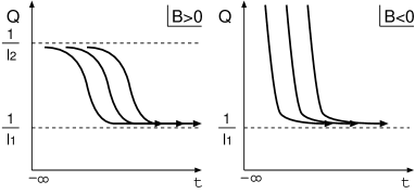
Figure 1: Classical solutions $Q(t)$ for $A>0$.

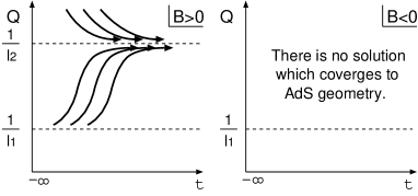
Figure 2: Classical solutions $Q(t)$ for $A<0$.

Figure 3: Result of the numerical calculation of classical solutions $Q(t)$ for the values $d=4$, $A=0.1$, $B=0.1$ and $l=1$ ($1/l_{1}=1$ and $1/l_{2}=6.24$).

Now we give a holographic RG interpretation to the above results. We first consider the AdS⁽¹⁾ solution. Eq. (3.10) expresses the equation of motion of a scalar field in the AdS background of radius $l$, with mass squared given by

$$m_{1}^{2} =-{2\over A}\left(2\Lambda l^{2}+{3B\over l^{2}}\right)$$

$$={2\over A}\left(d(d-1)-{6B\over l^{2}}\right).$$ (3.14)

Thus for $A>0$, the higher-derivative mode $Q$ is interpreted as a very massive scalar mode, and thus is coupled to a highly irrelevant operator around the fixed point since its scaling dimension is given by [2][3]

$$\Delta={d\over 2}+\sqrt{{d^{4}\over 4}+l^{2}m_{1}^{2}}\gg d.$$ (3.15)

This can also be understood from Fig. 1 which shows a rapid convergence of the RG flow to the fixed point $Q(t)=1/l$. On the other hand, for $A<0$, the mass squared of the higher-derivative mode is far below the unitary bound $-d^{2}/4l^{2}$ for a scalar mode in the AdS⁽¹⁾ geometry [3], and the scaling dimension becomes complex. Thus, in this case, the higher-derivative mode makes the AdS⁽¹⁾ geometry unstable, and a holographic RG interpretation cannot be given to such solution.

We then consider the AdS⁽²⁾. For $A>0$ and $B>0$ in Fig. 1, one can find that classical trajectories begin from AdS⁽²⁾ to AdS⁽¹⁾. In the context of the holographic RG, this means that the AdS⁽²⁾ solution $Q(t)=1/l_{2}$ corresponds to a multicritical point in the phase diagram of the boundary field theory. From (3.8) and (3.11), the mass squared of the mode $Q$ around the AdS⁽²⁾ can be calculated to be

$$m_{2}^{2}=-{2\over A}\left(d(d-1)-{6B\over l^{2}}\right),$$ (3.16)

and if this mass squared is above the unitarity bound,

$$l_{2}^{2}m_{2}^{2}=-{6B\over A}{d(d-1)l^{2}-6B\over d(d-1)l^{2}-3B}>-{d^{2}\over 4},$$ (3.17)

the scaling dimension of the corresponding operator is given by

$$\Delta ={d\over 2}+\sqrt{{d^{2}\over 4}+l_{2}^{2}m_{2}^{2}}$$

$$\cong{d\over 2}+\sqrt{{d^{2}\over 4}-{6B\over A}}.$$ (3.18)

For example, we consider the case where $d=4$, $a=b=0$ and $c>0$. In this case, $A=32c>0$ and $B=8c/3>0$, and thus the scaling dimension of $Q$ around the AdS⁽²⁾ is $\Delta\cong 2+\sqrt{7/2}$. It would be interesting to investigate which conformal field theory describes this fixed point.

We conclude this section with a comment on the $c$-theorem. In the block spin gauge, the function $Q^{d-1}(t)$ can be regarded as the $c$-function of the $d$-dimensional field theory [8]. Fig. 1 shows that it increases when $A>0$, but this does not contradict what the $c$-theorem says because in this case, the kinetic term of $Q(t)$ in the bulk action has a negative sign [see (3.4)].

4 Scalar Field with Higher-Derivative Interaction in Einstein Gravity

In this section, we consider a scalar field with higher-derivative interaction in Einstein gravity.

To simplify the discussion below, we consider the action

$$\mbox{\boldmath$S$}=\int_{M_{d+1}}d^{d+1}X\sqrt{\widehat{g}}\left[V(\phi)-\widehat{R}+{1\over 2}\widehat{g}^{\mu\nu}\partial_{\mu}\phi\partial_{\nu}\phi+{c\over 2}\left(\widehat{\nabla}^{2}\phi\right)^{2}\right]+2\int_{\Sigma_{d}}d^{d}xK,$$ (4.1)

where $\widehat{\nabla}$ is the covariant derivative defined by $\widehat{g}_{\mu\nu}$, and $c$ is a given small constant of the order of $\alpha^{\prime}$. Substituting the block spin gauge metric (2.5) into (4.1), $S$ becomes

$$S ={\mathcal{V}}_{d}\int_{t_{0}}L(\phi,\dot{\phi},\ddot{\phi};Q)$$

$$={\mathcal{V}}_{d}\int_{t_{0}}e^{-dt}\left\{{1\over Q}V(\phi)-d(d-1)Q+{Q\over 2}\dot{\phi}^{2}+{c\over 2}e^{2dt}Q\left[\left(e^{-dt}Q\dot{\phi}\right)^{\!\displaystyle{\cdot}}\,\right]^{2}\right\}.$$ (4.2)

As the Lagrangian contains $\ddot{\phi}$, it is convenient to treat this system in the Hamilton formalism [28]. Following the procedure given in Appendix A, we introduce a Lagrange multiplier $\pi$ and rewrite the action in the following equivalent form:

$$\mbox{\boldmath$S$}={\mathcal{V}}_{d}\int_{t_{0}}dt\left[\pi\left(\dot{\phi}-e^{dt}{\Phi\over Q}\right)+e^{-dt}\left({1\over Q}V(\phi)-d(d-1)Q+{Q\over 2}\dot{\phi}^{2}\right)+{c\over 2}e^{dt}Q\dot{\Phi}^{2}\right].$$ (4.3)

Then, making the Legendre transformation from $\dot{\Phi}$ to the conjugate momentum

$$\Pi=c\,e^{dt}Q\dot{\Phi},$$ (4.4)

we further rewrite the action into the first order form:

$$\mbox{\boldmath$S$}={\mathcal{V}}_{d}\int_{t_{0}}dt\left[\pi\dot{\phi}+\Pi\dot{\Phi}-H(\phi,\Phi,\pi,\Pi;Q)\right],$$ (4.5)

where

$$H(\phi,\Phi,\pi,\Pi;Q)=d(d-1)e^{-dt}Q+{1\over Q}\left[{e^{-dt}\over 2c}\Pi^{2}+e^{dt}\pi\Phi-e^{-dt}V(\phi)-{e^{dt}\over 2}\Phi^{2}\right].$$ (4.6)

In (4.5), $Q$ appears without time derivative, thus it can be easily solved to be

$$Q^{2}(\phi,\Phi,\pi,\Pi)={1\over d(d-1)}\left[{1\over 2c}\Pi^{2}-V(\phi)+e^{2dt}\left(\pi\Phi-{1\over 2}\Phi^{2}\right)\right],$$ (4.7)

and substituting this into the Hamiltonian (4.6), we obtain the final form of the Hamiltonian:

$$H(\phi,\Phi,\pi,\Pi)=2d(d-1)e^{-dt}Q(\phi,\Phi,\pi,\Pi).$$ (4.8)

The Hamilton equation is given by

$$Q\dot{\phi}=e^{dt}\Phi,\quad Q\dot{\Phi}={e^{-dt}\over c}\Pi,\quad Q\dot{\pi}=e^{-dt}V^{\prime}(\phi),\quad Q\dot{\Pi}=e^{dt}\left(\Phi-\pi\right).$$ (4.9)

As in the pure gravity case, we first look for the AdS solution which is given by $Q={\rm const.}$ If we set

$$V(\phi)\equiv-{d(d-1)\over l^{2}}+{\mu^{2}\over 2}\phi^{2},$$ (4.10)

the AdS solution which satisfies (4.7) and (4.9) is given by

$$Q=\frac{1}{l},\quad\phi=\Phi=\pi=\Pi=0.$$ (4.11)

We then expand the Hamilton equation (4.9) around the AdS solution (4.11) up to first order in variables:

$${1\over l}\dot{\phi}=e^{dt}\Phi,\quad{1\over l}\dot{\Phi}={e^{-dt}\over c}\Pi,\quad{1\over l}\dot{\pi}=e^{-dt}\mu^{2}\phi,\quad{1\over l}\dot{\Pi}=e^{dt}\left(\Phi-\pi\right).$$ (4.12)

This can be easily solved by performing the canonical transformation [28]

$$\begin{pmatrix}\phi\\ \Phi\\ \pi\\ \Pi\end{pmatrix}=a_{1}\begin{pmatrix}1&0&0&e^{dt}/M\\ 0&e^{-dt}M&1&0\\ 0&e^{-dt}cm^{2}M&cM^{2}&0\\ cm^{2}&0&0&e^{dt}cM\end{pmatrix}\begin{pmatrix}\widetilde{\phi}\\ \widetilde{\Phi}\\ \widetilde{\pi}\\ \widetilde{\Pi}\end{pmatrix},$$ (4.13)

with

$$a_{1}^{2}\equiv{1\over\sqrt{1-4c\mu^{2}}},\quad M^{2}\equiv{1\over 2c}\left(1+\sqrt{1-4c\mu^{2}}\right),\quad m^{2}\equiv{1\over 2c}\left(1-\sqrt{1-4c\mu^{2}}\right).$$ (4.14)

Then, the linearized Hamilton equation (4.12) is decomposed into two sets of independent equations,

$$\begin{cases}\dot{\widetilde{\phi}}&=le^{dt}\widetilde{\pi},\\ \dot{\widetilde{\pi}}&=-lm^{2}e^{-dt}\widetilde{\phi},\end{cases}\qquad\begin{cases}\dot{\widetilde{\Phi}}&=le^{dt}\widetilde{\Pi},\\ \dot{\widetilde{\Pi}}&=-lM^{2}e^{-dt}\widetilde{\Phi},\end{cases}$$ (4.15)

which are equivalent to

$$\ddot{\widetilde{\phi}}-d\dot{\widetilde{\phi}}-l^{2}m^{2}\widetilde{\phi} =0,$$ (4.16)

$$\ddot{\widetilde{\Phi}}-d\dot{\widetilde{\Phi}}-l^{2}M^{2}\widetilde{\Phi} =0,$$ (4.17)

respectively. These are nothing but the equation of motion of two scalar fields with mass squared $m^{2}$ and $M^{2}$, respectively, in the AdS background $Q=1/l$. In particular, $\widetilde{\Phi}$ acquires large mass when $c>0$ since its mass squared $M^{2}$ becomes $\sim 1/c\sim 1/\alpha^{\prime}\gg m^{2}$. Thus the bulk scalar field $\widetilde{\Phi}$ is coupled to a highly irrelevant operator at the boundary. If we assume that $\widetilde{\phi}$ is a relevant coupling, i.e. $-d^{2}/4l^{2}<m^{2}<0$, then the RG flow near the fixed point, $\phi=\Phi=0$, will converges rapidly to the renormalized trajectory given by $\widetilde{\phi}=0$ [see Fig. 4].

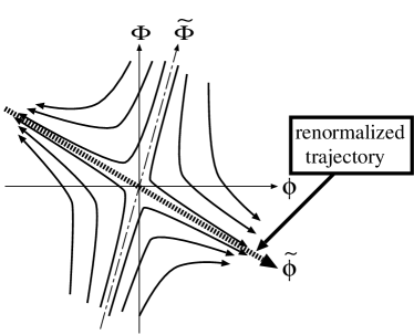
Figure 4: The RG flow of the coupling constants $(\phi,\Phi)$ near the fixed point $\phi=0$ and $\Phi=0$.

On the other hand, when $c<0$, the mass squared of the scalar mode $\widetilde{\Phi}$ is far below the unitarity bound, thus the AdS geometry becomes unstable. In this case, as in the pure gravity case with $A<0,B<0$, the holographic RG interpretation of the higher-derivative system is not possible.

5 Application to a Model of Universe with Positive Cosmological Constant

In this section, we apply our analysis of higher-derivative pure gravity to systems of Lorentzian gravity with positive cosmological constant. There, as classical solutions, one can have de Sitter solutions instead of AdS solutions. We shall see that, in a certain region of coefficients of higher-derivative terms, there are two de Sitter solutions as well as a kink solution which interpolates these two de Sitter geometries.

We consider the following action of higher-derivative pure gravity in a $(d+1)$-dimensional Lorentzian Manifold:

$$\mbox{\boldmath$S$}=\int d^{d+1}X\sqrt{-\widehat{g}}\biggl{(}-2\Lambda+\widehat{R}-a\widehat{R}^{2}-b\widehat{R}_{\mu\nu}^{2}-c\widehat{R}_{\mu\nu\rho\sigma}^{2}\biggr{)}.$$ (5.1)

Our discussion is completely parallel to the one given in §3. We take the block spin gauge metric

$$ds^{2}=-{1\over Q^{2}}dt^{2}+e^{2t}\delta_{ij}dx^{i}dx^{j},$$ (5.2)

where we flipped the sign of the exponent to describe the expanding universe. If $Q=1/l=$const., (5.2) expresses de Sitter space-time of radius $l$. With the metric (5.2), the action (5.1) becomes

$$\mbox{\boldmath$S$}={\mathcal{V}}_{d}\int dte^{dt}\left[-{2\Lambda\over Q}-d(d-1)Q-{A\over 2}Q\dot{Q}^{2}+BQ^{3}\right],$$ (5.3)

where $A$ and $B$ are again given by (3.5). This action gives the equation of motion for $Q$,

$$Q\ddot{Q}+{1\over 2}\dot{Q}^{2}+dQ\dot{Q}=-{1\over A}\left({2\Lambda\over Q^{2}}-d(d-1)+3BQ^{2}\right),$$ (5.4)

which is nothing but (3.6) if we make a change there as $\Lambda\to-\Lambda$ and $t\to-t$. By parametrizing the cosmological constant as

$$\Lambda={d(d-1)\over 2l^{2}}-{3B\over l^{4}},$$ (5.5)

the de Sitter solutions are obtained from (5.4) as

$$Q^{2}=\begin{cases}\displaystyle{~{}~{}~{}~{}~{}~{}~{}{1\over l^{2}}}\!&\displaystyle{\equiv\,{1\over l_{1}^{2}}}\,\,,\vspace{2mm}\\ \displaystyle{{d(d-1)\over 3B}-{1\over l^{2}}}\!&\displaystyle{\equiv\,{1\over l_{2}^{2}}}\,\,,\end{cases}$$ (5.6)

where the solution $Q=1/l_{2}$ exists only when $B>0$. We call the solution $Q=1/l_{i}$ the dS${}^{(i)}\,\,(i=1,2)$ solution, respectively.

As we did in §3, we next examine the perturbation of solutions around these de Sitter solutions. By writing $Q(t)$ as

$$Q(t)={1\over l_{i}}+X_{i}(t),$$ (5.7)

the equation of motion (5.4) is linearized as

$$\ddot{X}_{i}+d\dot{X}_{i}-\lambda_{i}X_{i}=0,$$ (5.8)

where

$$\begin{cases}\displaystyle{\,\lambda_{1}}&\displaystyle{\!\!=\,{2\over A}\left(d(d-1)l^{2}-6B\right)}\,\,,\vspace{2mm}\\ \displaystyle{\,\lambda_{2}}&\displaystyle{\!\!=\,-\,{6B\over A}\cdot{d(d-1)l^{2}-6B\over d(d-1)l^{2}-3B}}\,\,.\end{cases}$$ (5.9)

This equation is actually the time reversal of the linearized equation in the AdS case [see (3.10), (3.13)], and thus we readily find from Fig. 1 and Fig. 2 that the general classical solutions behave as in Fig. 5 and Fig. 6. Note that we now can have a meaningful solution when $A<0,\,B<0$, since we no longer need to restrict our consideration to the systems with finite classical action.

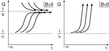
Figure 5: Classical solutions $Q(t)$ for $A>0$. The dS⁽¹⁾ solution is unstable, and the space-time converges to the dS⁽²⁾ geometry if it exists.

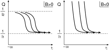
Figure 6: Classical solutions $Q(t)$ for $A<0$. The dS⁽¹⁾ solution is now stable, and thus the space-time converges to the dS⁽¹⁾ geometry. If the solution dS⁽²⁾ exists, there are solutions which describe time evolution from dS⁽²⁾ to dS⁽¹⁾.

The interesting case is when $B>0$. Then there is a solution which describes time evolution of space-time from a de Sitter geometry to another de Sitter geometry. Since the Hubble parameter is defined by $H(\tau)=\dot{R}(\tau)/R(\tau)$ for a metric $ds_{d+1}^{2}=-d\tau^{2}+R^{2}(\tau)ds_{d}^{2},$ one understands that the higher-derivative mode $Q$ is nothing but the Hubble parameter:

$$H(\tau)=Q(t(\tau)).$$ (5.10)

Thus, the solutions for $B>0$ in Fig. 5 and Fig. 6 describe a universe in which the Hubble parameter changes rapidly from a constant to a constant. Since we are assuming that the coefficients of the curvature squared terms are of the string scale, the difference between the two Hubble constants is magnificently large. Such solutions can always exist in all dimensionality but four $(d=3)$ because $B\neq 0$ when $d\neq 3$. The absence of such solutions in four-dimensional space-time might be remedied by coupling an extra matter field to gravity.

6 Conclusion

In this paper, we investigated higher-derivative gravity systems. We introduced the block spin gauge (2.5) in which time evolution can be regarded directly as change of the unit length in the $d$-dimensional time slice. We considered (1) higher-derivative pure gravity and also (2) a scalar field with higher-derivative interaction in Einstein gravity. We examined classical solutions in the block spin gauge and gave a holographic RG interpretation to the higher-derivative modes.

We showed the existence of AdS solutions for both systems (1) and (2), and discussed their stability. Under the request that the bulk fields be regular in the region far away from the boundary, we found that the stability of the AdS solutions depends on the values of the coefficients of higher-derivative terms. In the region of stable AdS, the higher-derivative mode can be interpreted as a very massive scalar field in the AdS background. Thus, in the context of the holographic RG, it is coupled to a highly irrelevant operator at the boundary. On the other hand, in the region of unstable AdS, the higher-derivative mode acquires large negative mass squared which is far below the unitarity bound in AdS gravity. In this case, it is difficult to give a holographic RG interpretation.

For higher-derivative pure gravity, in particular, there is a region in which one can have two AdS solutions. In that region, one can also have a kink solution which describes a flow from an AdS geometry to another AdS geometry. (This is when $B>0$ in the Fig. 1 and Fig. 2.) In particular, for $A>0$ and $B>0$, the flow starts from the AdS geometry of much smaller radius (of the string scale). This describes an RG flow from a non-trivial multicritical point to another fixed point, the latter of which governs the universality class described by pure Einstein gravity. The appearance of such multicritical point is characteristic of the holographic RG for an $R^{2}$-gravity system.

As an application of our analysis, we investigated $(d+1)$-dimensional Lorentzian higher-derivative gravity with positive cosmological constant. We found that there is a solution which describes time evolution from a de Sitter geometry to another de Sitter geometry in a certain region of the coefficients of the curvature squared terms. Along the solution, the value of the Hubble parameter changes drastically.

Finally, we comment on the meaning of the mixed boundary conditions which were adopted in [28] (see also Appendix A below). As mentioned above, the higher-derivative mode near the stable AdS solution is coupled to a highly irrelevant operator at the boundary, so the RG flow around the corresponding fixed point converges rapidly to the renormalized trajectory on which the higher-derivative mode does not flow. We shall see that one can actually pick up the renormalized trajectory by adopting the mixed boundary conditions.

In the case of pure gravity, the fixed point is given by the solution

$$Q={1\over l}.$$ (6.1)

On the other hand, from the Lagrangian (3.4), the conjugate momentum for $Q$ is calculated as

$$P=-Ae^{-dt}\dot{Q}+\biggl{[}4d\bigl{(}d(d+1)a+db+2c\bigr{)}+3d\bigl{(}d^{2}x_{3}+dx_{4}+x_{5}\bigr{)}\bigg{]}Q^{2}$$ (6.2)

Thus, the fixed point (6.1) can be picked up by the equation $P=0$ if we set the coefficients as in [28]:

$$d^{2}x_{3}+dx_{4}+x_{5}=-{4\over 3}\bigl{(}d(d+1)a+db+2c\bigr{)}.$$ (6.3)

In other words, with the use of the freedom to add total derivative terms to the action, the coefficients can be chosen such that the equation $P=0$ directly gives the fixed point. Note that the total derivative terms can be interpreted as the generating function of a canonical transformation which shifts the value of the conjugate momentum.

The situation does not change for a scalar field coupled to Einstein gravity with higher-derivative interaction. When $\widetilde{\phi}$ is a relevant coupling, the renormalized trajectory is given by $\widetilde{\Phi}=0$, which is equivalent to $\widetilde{\Pi}=0$. On the other hand, from the canonical transformation (4.13), $\widetilde{\Pi}$ is expressed as

$$\widetilde{\Pi}=\sqrt{1-4c\mu^{2}}\biggl{(}\Pi-cm^{2}\phi\biggr{)}.$$ (6.4)

Thus, if we add the term

$${d\over dt}F(\phi,\Phi)\equiv{d\over dt}\biggl{(}cm^{2}\phi\Phi\biggr{)}$$ (6.5)

to the Lagrangian (4.2) (or equivalently $cm^{2}\widehat{\nabla}^{\mu}(\phi\,\partial_{\mu}\phi)$ to the Lagrangian density), we can shift the conjugate momenta as

$$\pi\to\pi+cm^{2}\Phi,\quad\Pi\to\Pi+cm^{2}\phi,$$ (6.6)

so that we have $\widetilde{\pi}\propto\pi$ and $\widetilde{\Pi}\propto\Pi$. This enables us to pick up the renormalized trajectory with the mixed boundary conditions ($\Pi=0$).

Appendix A General Theory of Higher-Derivative Systems

In this appendix, we give a brief review on classical mechanics of higher-derivative systems with the action

$$\mbox{\boldmath$S$}{}[q]=\int_{t_{0}}^{t_{1}}dt\,L(q,\dot{q},\ddot{q}).$$ (A.1)

The variational principle gives the Euler-Lagrange equation:

$$0={d^{2}\over dt^{2}}\left({\partial L\over\partial\ddot{q}}\right)-{d\over dt}\left({\partial L\over\partial\dot{q}}\right)+{\partial L\over\partial q}.$$ (A.2)

This system can also be investigated in the Hamilton formalism: We first introduce a Lagrange multiplier $p$ to treat $\dot{q}$ as a new canonical variable $Q$:

$$L\left(q,\dot{q},\ddot{q}\right)\to p\,(\dot{q}-Q)+L\left(q,Q,\dot{Q}\right).$$ (A.3)

We call $Q$ the higher-derivative mode. Then, by making the Legendre transformation from $\dot{Q}$ to the conjugate momentum $P\equiv\partial L/\partial\dot{Q}$, this action can be rewritten into the first order form:

$$\mbox{\boldmath$S$}{}[q,Q,p,P]=\int_{t_{0}}^{t_{1}}dt\,\left[p\,\dot{q}+P\dot{Q}-H(q,Q;p,P)\right],$$ (A.4)

with the Hamiltonian

$$H(q,Q;q,P)\equiv p\,Q+P\cdot f(q,Q,P)-L(q,Q,f(q,Q,P)).$$ (A.5)

Here $f(q,Q,P)$ in (A.5) is obtained by solving $P=\partial L(q,Q,f)/\partial f=P(q,Q,f)$ in $f$. Again by the variational principle, we obtain the Hamilton equation

$$\dot{q}={\partial H\over\partial p},\quad\dot{Q}={\partial H\over\partial P},\quad\dot{p}=-{\partial H\over\partial q},\quad\dot{P}=-{\partial H\over\partial Q},$$ (A.6)

together with the boundary conditions

$$p\,\delta q+P\delta Q=0\quad(t=t_{0},t_{1}).$$ (A.7)

One can easily check that the Hamilton equation (A.6) is equivalent to the Euler-Lagrange equation (A.2).

The boundary condition (A.7) is satisfied by the Dirichlet boundary conditions

$$\delta q=0\,,\quad\delta Q=0\quad(t=t_{0},t_{1})\,,$$ (A.8)

or the Neumann boundary conditions

$$p=0\,,\quad P=0\quad(t=t_{0},t_{1})\,,$$ (A.9)

for each variable $q$ and $Q$. A choice of interest for us is to take the mixed boundary conditions, that is, we set the Dirichlet conditions for $q$ ($q(t_{0})=q_{0}$ and $q(t_{1})=q_{1}$) and the Neumann conditions for $Q$ ($P(t_{0})=P(t_{1})=0$). Then, if we substitute such classical solution into the bulk action $S$, the resulting classical action is a function only of the boundary values of the light mode $q$; $\mbox{\boldmath$S$}[q(t),Q(t),p(t),P(t)]\equiv S(q_{0},t_{0};q_{1},t_{1})$.

In [28], the mixed boundary conditions were adopted to establish the holographic principle in higher-derivative gravity systems. In fact, if we set the mixed boundary conditions for a bulk field $\phi(x,t)$ as $\phi(x,t\!=\!t_{a})=\phi_{a}(x)$ and $\Pi(x,t\!=\!t_{a})=0$ $(a=0,1)$, and carefully choose $\phi_{1}(x)$ such that the classical action is finite in the limit $t_{1}\to+\infty$, then the classical action becomes a functional only of $\phi_{0}(x)$ and $t_{0}$, $S[\phi_{0}(x),t_{0}]$. This may be interpreted as the fixed point action with the bare coupling $\phi_{0}$ at the UV cutoff $\Lambda=\exp(-t_{0})$, in the presence of an irrelevant operator corresponding to the higher-derivative mode of $\phi$. In other words, the classical solution under the mixed boundary conditions may describe an RG flow of the coupling constant along the renormalized trajectory. The main text of the present paper actually supports this idea.

Appendix B Higher-Derivative Pure Gravity without Gauge Fixing

In this appendix, we verify that $Q(t)$ in the block spin gauge metric is actually the higher-derivative mode in the sense given in Appendix A. We give a discussion by explicitly solving the equation of motion of (3.1) without assuming any particular form for the variables appearing in the metric (2.2).

Substituting (2.2) into (3.1), we obtain the Lagrangian of this system:

$$L\biggl{(}q, {\dot{q}\over N},\left({\dot{q}\over N}\right)^{\!\!\displaystyle{\cdot}};N\biggr{)}$$

$$=Ne^{-dq(\tau)}\left\{2\Lambda-d(d-1)\left(\dot{q}(\tau)\over N\right)^{2}-{A\over 2N^{2}}\left[\left(\dot{q}(\tau)\over N\right)^{\!\!\displaystyle{\cdot}}\,\right]^{2}+B\left(\dot{q}(\tau)\over N\right)^{4}\right\},$$ (B.1)

where $\cdot\equiv d/d\tau$. Following the discussion of Appendix A, we introduce a Lagrange multiplier $p$ to set

$$\widetilde{Q}(\tau)={\dot{q}(\tau)\over N}.$$ (B.2)

The Lagrangian then becomes

$$L=p\left(\dot{q}-N\widetilde{Q}\right)-{A\over 2N}e^{-dq}\dot{\widetilde{Q}}^{2}+Ne^{-dq}\left(2\Lambda-d(d-1)\widetilde{Q}^{2}+B\widetilde{Q}^{4}\right).$$ (B.3)

Since $N$ is not dynamical, its classical value can be easily found to be

$$N=\sqrt{A\dot{\widetilde{Q}}^{2}\over 2p\widetilde{Q}e^{dq}-2\left(2\Lambda-d(d-1)\widetilde{Q}^{2}+B\widetilde{Q}^{4}\right)}.$$ (B.4)

Substituting this into the Lagrangian, we obtain the action for this system:

$$\mbox{\boldmath$S$}=\int_{\tau_{0}}d\tau\left\{p\dot{q}+2\sqrt{{A\over 2}e^{-dq}\dot{\widetilde{Q}}^{2}\left[p\widetilde{Q}-e^{-dq}\left(2\Lambda-d(d-1)\widetilde{Q}^{2}+B\widetilde{Q}^{4}\right)\right]}\right\}.$$ (B.5)

Now we impose the condition (2.4) to $q(\tau)$, which allows us to change the integration variable from $\tau$ to $q$:

$$\mbox{\boldmath$S$}=\int_{q_{0}}dq\left\{p+2\sqrt{{A\over 2}e^{-dq}\dot{Q}^{2}\biggl{[}pQ-e^{-dq}\left(2\Lambda-d(d-1)Q^{2}+BQ^{4}\right)\biggr{]}}\right\},$$ (B.6)

where

$$Q(q)\equiv\widetilde{Q}(\tau(q)),$$ (B.7)

and $\cdot$ is now understood to represent $d/dq$. The action (B.6) can be further simplified by substituting the classical value of $p$, and we finally obtain the action

$$\mbox{\boldmath$S$}=\int_{q_{0}}dq\,\,e^{-dq}\left(-\frac{A}{2}\,Q\,\dot{Q}^{2}+\frac{2\Lambda}{Q}-d(d-1)Q+BQ^{3}\right).$$ (B.8)

This is nothing but the action (3.4) in the block spin gauge if we rewrite $q$ as $t$. Thus we can conclude that $Q(t)$ in the block spin gauge metric (2.5) corresponds to the higher-derivative mode introduced in Appendix A, and is related to the variable $q$ in the temporal gauge ($N=1)$ as

$$Q(t)={dq(\tau)\over d\tau}\bigg{|}_{\tau=q^{-1}(t)}.$$ (B.9)

Using the same procedure, we can also derive (4.8) from the temporal gauge metric (2.3) under the condition (2.4).

References

- [1] J. Maldacena, “The large limit of superconformal field theories and supergravity,” Adv. Theor. Math. Phys. 2 (1998) 231, hep-th/9711200.
- [2] S. S. Gubser, I. R. Klebanov and A. M. Polyakov, “Gauge Theory Correlators from Non-Critical String Theory,” Phys. Lett. B428 (1998) 105, hep-th/9802109.
- [3] E. Witten, “Anti De Sitter Space And Holography,” Adv. Theor. Math. Phys. 2 (1998) 253, hep-th/9802150.
- [4] O. Aharony, S. S. Gubser, J. Maldacena, H. Ooguri and Y. Oz, “Large N Field Theories, String Theory and Gravity,” hep-th/9905111, and references therein.
- [5] L. Susskind and E. Witten, “The holographic bound in anti-de Sitter space,” hep-th/9805114.
- [6] E. T. Akhmedov, “A remark on the AdS/CFT correspondence and the renormalization group flow,” Phys.Lett. B442 (1998) 152, hep-th/9806217.
- [7] E. Alvarez and C. Gomez, “Geometric Holography, the Renormalization Group and the c-Theorem,” Nucl.Phys. B541 (1999) 441, hep-th/9807226.
- [8] D.Z. Freedman, S.S. Gubser, K. Pilch and N.P. Warner, “Renormalization Group Flows from Holography–Supersymmetry and a c-Theorem,” hep-th/9904017.
- [9] L. Girardello, M. Petrini, M. Porrati and A. Zaffaroni, “Novel Local CFT and Exact Results on Perturbations of N=4 Super Yang Mills from AdS Dynamics,” J.High Energy Phys. 12 (1998) 022, hep-th/9810126.
- [10] L. Girardello, M. Petrini, M. Porrati and A. Zaffaroni “The Supergravity Dual of N=1 Super Yang-Mills Theory,” Nucl.Phys. B569 (2000) 451, hep-th/9909047.
- [11] M. Porrati and A. Starinets, “RG Fixed Points in Supergravity Duals of 4-d Field Theory and Asymptotically AdS Spaces,” Phys.Lett. B454 (1999) 77, hep-th/9903085.
- [12] V. Balasubramanian and P. Kraus, “Spacetime and the Holographic Renormalization Group,” Phys. Rev. Lett. 83 (1999) 3605, hep-th/9903190.
- [13] K. Skenderis and P. K. Townsend, “Gravitational Stability and Renormalization-Group Flow,” Phys.Lett. B468 (1999) 46, hep-th/9909070.
- [14] O. DeWolfe, D. Z. Freedman, S. S. Gubser and A. Karch, “Modeling the fifth dimension with scalars and gravity,” Phys. Rev. D62 (2000) 046008. hep-th/9909134.
- [15] M. Henningson and K. Skenderis, “The Holographic Weyl anomaly,” J.High Energy Phys. 07 (1998) 023, hep-th/9806087.
- [16] J. de Boer, E. Verlinde and H. Verlinde, “On the Holographic Renormalization Group,” hep-th/9912012.
- [17] M. Fukuma, S. Matsuura and T. Sakai, “A Note on the Weyl Anomaly in the Holographic Renormalization Group,” Prog. Theor. Phys. 104 (2000) 1089, hep-th/0007062.
- [18] M. Fukuma and T. Sakai, “Comment on Ambiguities in the Holographic Weyl Anomaly,” Mod. Phys. Lett. A15 (2000) 1703, hep-th/0007200.
- [19] S. Corley, “A Note on Holographic Ward Identities,” Phys. Lett. B484 (2000) 141, hep-th/0004030.
- [20] J. Kalkkinen and D. Martelli, “Holographic Renormalization Group with Fermions and Form Fields,” hep-th/0007234.
- [21] J. Kalkkinen, D. Martelli and W. Mueck, “Holographic Renormalisation and Anomalies,” hep-th/0103111.
- [22] S. Nojiri, S. D. Odintsov and S. Ogushi, “Holographic renormalization group and conformal anomaly for AdS9/CFT8 correspondence ,” Phys. Lett. 500 (2001) 199, hep-th/0011182.
- [23] D. Anselmi and A. Kehagias, “Subleading Corrections and Central Charges in the AdS/CFT Correspondence,” Phys. Lett. B455 (1999) 155 , hep-th/9812092.
- [24] O. Aharony, J. Pawelczyk, S. Theisen and S. Yankielowicz, “A Note on Anomalies in the AdS/CFT correspondence,” Phys. Rev. D60 (1999) 066001, hep-th/9901134.
-
[25]
S. Nojiri and S. D. Odintsov,
“On the conformal anomaly from higher derivative gravity
in AdS/CFT correspondence,”
Int. J. Mod. Phys. A15 (2000) 413
hep-th/9903033;
S. Nojiri and S. D. Odintsov, “Finite gravitational action for higher derivative and stringy gravity,” Phys. Rev. D62 (2000) 064018 hep-th/9911152. - [26] M. Blau, K. S. Narain and E. Gava “On Subleading Contributions to the AdS/CFT Trace Anomaly,” J.High Energy Phys. 9909 (1999) 018, hep-th/9904179.
- [27] A. Bilal and C.-S. Chu, “A Note on the Chiral Anomaly in the AdS/CFT Correspondence and Correction,” Nucl. Phys. B562 (1999) 181, hep-th/9907106.
- [28] M. Fukuma, S. Matsuura and T. Sakai, “Higher-Derivative Gravity and the AdS/CFT Correspondence,” Prog. Theor. Phys. 105 (2001) 1017, hep-th/0103187.
-
[29]
S. Naka,
“Difference Equation and Dual Resonance Model,”
Prog. Theor. Phys. 48 (1972) 1024;
M. Kato, “Particle theories with minimum observable length and open string theory,” Phys. Lett. B245 (1990) 43. -
[30]
A. Fayyazuddin and M. Spalinski
“Large Superconformal Gauge Theories and Supergravity
Orientifolds,”
Nucl.Phys. B535 (1998) 219,
hep-th/9805096;
O. Aharony, A. Fayyazuddin and J. Maldacena, “The Large Limit of Field Theories from Three Branes in F-theory,” J.High Energy Phys. 9807 (1998) 013, hep-th/9806159. - [31] M. J. Duff, “Twenty Years of the Weyl Anomaly,” Class. Quant. Grav. 11 (1994) 1387, hep-th/9308075.
-
[32]
D. G. Boulware,
“Quantization of Higher Derivative Theoreis of Gravity,”
in Quantum theory of gravity : essays in honor of the 60th birthday
of Bryce S. DeWitt, ed. S. M. Christensen (Adam Hilger Ltd, Bristol, 1984), P.267.
S. W. Hawking and J. C. Luttrell, “Higher Derivative in Quantum Cosmology (I). The isotropic case,” Nucl. Phys. B247 (1984) 250. - [33] S. Nojiri and S. D. Odintsov, “Brane World Inflation Induced by Quantum Effects,” Phys. Lett. B484 (2000) 119, hep-th/0004097.
- [34] G. W. Gibbons and S. W. Hawking, “Action Integrals and Partition Functions in Quantum Gravity,” Phys. Rev. D15 (1977) 2752.
- [35] R. C. Myers, “Higher-derivative gravity, surface terms, and string theory,” Phys. Rev. D36 (1987) 392.
-
[36]
S. Nojiri and S. D. Odintsov,
“Brane-World Cosmology in Higher Derivative Gravity or Warped
Compactification in the Next-to-leading Order of AdS/CFT Correspondence,”
J.High Energy Phys. 0007 (2000) 049,
hep-th/0006232,
S. Nojiri, S. D. Odintsov and S. Ogushi, “Dynamical Branes from Gravitational Dual of Superconformal Field Theory,” hep-th/0010004,
S. Nojiri, S. D. Odintsov, S. Ogushi, “Holographic entropy and brane FRW-dynamics from AdS black hole in d5 higher derivative gravity,” hep-th/0105117.