Stability of two-fermion bound states in the explicitly covariant Light-Front Dynamics

1 Introduction

The system of two bound fermions covers a huge number of interesting problems from atomic, nuclear and subnuclear physics. It is one of the most difficult problems in field theory due to the fact that bound states necessarily involve an infinite number of diagrams. We studied this problem in the framework of the explicitly covariant light-front dynamics [1] (CLFD). In this approach, the state vector is defined on an hyperplane given by the invariant equation $\omega\cdot x=0$ with $\omega^{2}=0$. The standard light-front, reviewed in [2], is recovered for $\omega=(1,0,0,-1)$. The CLFD equations have been solved exactly for a two fermion system with different boson exchange ladder kernels [3, 4]. We have considered separately the usual couplings between two fermions (scalar, pseudo-scalar, pseudo-vector, and vector) and we were interested in states with given angular momentum and parity $J^{\pi}=0^{\pm},1^{\pm}$. Each coupling leads to a system of integral equations, which in practice are solved on a finite momentum domain $[0;k_{max}]$. If the solutions necessarily exist when the integration domain is finite – for the kernels are compact, it is not a priori obvious that the equations admit stable solutions when $k_{max}$ goes to infinity. Particular attention must therefore be paid to the stability of the equations relative to the cutoff $k_{max}$. We develop hereafter an analytical method to study the cutoff dependence of the equations and to determine whether they need to be regularized or not.

The method will here be detailed for a $J=0^{+}$ state in the Yukawa model but it can be applied to any coupling. Results will be presented for scalar and pseudo-scalar exchange. This latter furthermore exhibits some strange particularities which will be discussed.

2 Scalar exchange

Let us consider a system of two fermions in a $J^{\pi}=0^{+}$ state, bound by a scalar exchange, whose Lagrangian density is given by ${\cal{L}}=g_{s}\bar{\Psi}\Phi\Psi$. Its wave function, constructed using all possible spin structures, is determined in the $0^{+}$ case by two components [6], $f_{1}$ and $f_{2}$, which depend on the two scalar variables $k$ and $\theta$:

$$\psi={1\over\sqrt{2}}w^{{\dagger}}_{\sigma_{2}}\left(f_{1}+i{\vec{\sigma}\cdot[\vec{k}\times\hat{n}]\over k\sin\theta}f_{2}\right)\sigma_{y}w^{{\dagger}}_{\sigma_{1}}$$

$\vec{k}$ is the momentum of one particle in the system of reference where $\vec{k}_{1}+\vec{k}_{2}=0$, $\hat{n}$ is the spatial part of the normal $\omega$ to the light-front plane, $\theta$ is the angle between $\vec{k}$ and $\hat{n}$, and $w$ is the two component spinor. The appearence of a second component compared to the non relativistic case is due to vector $\hat{n}$, which induces additional spin structures.

$f_{1}$ and $f_{2}$ satisfy the system of coupled equations :

$$\left[M^{2}-4(k^{2}+m^{2})\right]f_{1}(k,\theta)$$ (1)

$$= \frac{m^{2}}{2\pi^{3}}\int\left[K_{11}f_{1}(k^{\prime},\theta^{\prime})+K_{12}f_{2}(k^{\prime},\theta^{\prime})\right]\frac{d^{3}k^{\prime}}{\varepsilon_{k^{\prime}}}$$

$$\left[M^{2}-4(k^{2}+m^{2})\right]f_{2}(k,\theta)$$

$$= \frac{m^{2}}{2\pi^{3}}\int\left[K_{21}f_{1}(k^{\prime},\theta^{\prime})+K_{22}f_{2}(k^{\prime},\theta^{\prime})\right]\frac{d^{3}k^{\prime}}{\varepsilon_{k^{\prime}}}$$

$M^{2}$ si the total mass squared of the system, $m$ is the constituent mass and $\varepsilon_{k}=\sqrt{\vec{k}^{2}+m^{2}}$. The kernels $K_{ij}$ result from a first integration of more elementary quantities:

$$K_{ij}(k,\theta;k^{\prime},\theta^{\prime}) = \int_{0}^{2\pi}{\kappa_{ij}\over(Q^{2}+\mu^{2})m^{2}\varepsilon_{k}\varepsilon_{k^{\prime}}}{d\varphi^{\prime}\over 2\pi},$$

where $\kappa_{ij}$ depend on the type of coupling. The analytical expressions of $\kappa_{ij}$ for the scalar coupling, read

$$\kappa^{S}_{11} = -\alpha\pi\left[2k^{2}k^{\prime 2}+3k^{2}m^{2}+3k^{\prime 2}m^{2}+4m^{4}\right.$$

$$-2kk^{\prime}\varepsilon_{k}\varepsilon_{k^{\prime}}\cos\theta\cos\theta^{\prime}$$

$$\left.-kk^{\prime}(k^{2}+k^{\prime 2}+2m^{2})\sin\theta\sin\theta^{\prime}\cos\varphi^{\prime}\right]$$

$$\kappa^{S}_{12} = -\alpha\pi m(k^{2}-k^{\prime 2})\left(k^{\prime}\sin\theta^{\prime}+k\sin\theta\cos\varphi^{\prime}\right)$$

$$\kappa^{S}_{21} = -\alpha\pi m(k^{\prime 2}-k^{2})\left(k\sin\theta+k^{\prime}\sin\theta^{\prime}\cos\varphi^{\prime}\right)$$

$$\kappa^{S}_{22} = -\alpha\pi\left[\left(2k^{2}k^{\prime 2}+3k^{2}m^{2}+3k^{\prime 2}m^{2}+4m^{4}\right.\right.$$ (2)

$$\left.-2kk^{\prime}\varepsilon_{k}\varepsilon_{k^{\prime}}\cos\theta\cos\theta^{\prime}\right)\cos\varphi^{\prime}$$

$$\left.-kk^{\prime}(k^{2}+k^{\prime 2}+2m^{2})\sin\theta\sin\theta^{\prime}\right]$$

In practice, the integration region over the momenta is reduced to a finite domain $[0,k_{max}]$. The kinematical term $[M^{2}-4(k^{2}+m^{2})]$ on l.h.s. of equation (1) does not generate any singularity and the kernels $K_{ij}$ are smooth functions of the $\theta$ variable. Thus, the stability of the solution depends only on the asymptotical behavior of the kernels in the $(k,k^{\prime})$ plane.

Variables $(k,k^{\prime})$ can tend to infinity following different directions: for a fixed value of $k$, $K_{11}$ decreases as $1/k^{\prime}$, and vice versa. As the integration volume contains the factor $\varepsilon_{k^{\prime}}$, this means that the total kernel decreases as $1/k^{\prime 2}$, that is like a Yukawa potential. In contrast, $K_{22}$ does not decrease in any direction of the $(k,k^{\prime})$ plane, but tends to a positive constant with respect to $k$ and $k^{\prime}$. $K_{22}$ is thus asymptotically repulsive and does not generate any unstability. In the domain where both $k,k^{\prime}$ tend to infinity with a fixed ratio ${k^{\prime}\over k}=\gamma$, it is useful to introduce the functions $A_{ij}$ defined by

$$K_{ij}=-\frac{\pi\alpha}{m^{2}}\left\{\begin{array}[]{ll}\sqrt{\gamma}\;A_{ij}(\theta,\theta^{\prime},\gamma)&\mbox{if $\gamma\leq 1$}\\ {1\over\sqrt{\gamma}}\;A_{ij}(\theta,\theta^{\prime},1/\gamma)&\mbox{if $\gamma\geq 1$}\end{array}\right.$$

Since $K_{22}$ is repulsive and does not generate any collapse, we consider only the first channel. We have

$$A_{11}(\theta,\theta^{\prime},\gamma)=\frac{1}{\sqrt{\gamma}}\int_{0}^{2\pi}\frac{d\varphi^{\prime}}{2\pi}{1\over D}\times$$

$$\left\{2\gamma(1-\cos\theta\cos\theta^{\prime})-(1+\gamma^{2})\sin\theta\sin\theta^{\prime}\cos\varphi^{\prime}\right\}$$

where

$$D = (1+\gamma^{2})(1+|\cos\theta-\cos\theta^{\prime}|-\cos\theta\cos\theta^{\prime})$$

$$- 2\gamma\sin\theta\sin\theta^{\prime}\cos\varphi^{\prime}$$

Let us now majorate the function $A_{11}$. For fixed $\gamma$, the maximum of $A_{11}$ is achieved at $\theta=\theta^{\prime}$ and for any $\theta=\theta^{\prime}$ it reads: $A_{11}(\theta=\theta^{\prime},\gamma)=\alpha^{\prime}\sqrt{\gamma}$. The maximum value of kernel $K_{11}$ is thus reached for $\gamma=1$. The majorated kernel obtained this way coincides with the non-relativistic potential $U(r)=-\alpha^{\prime}/r^{2}$ in the momentum space with $\alpha^{\prime}=\alpha/(2m\pi)$. As well known [7], for this potential, the binding energy does not depend on cutoff if $\alpha^{\prime}<\alpha_{cr}=1/(4m)$ what restricts the coupling constant to: $\alpha<\pi/2$. If $\alpha^{\prime}>1/(4m)$, the binding energy is cutoff dependent and tends to $-\infty$ when $k_{max}\to\infty$. A finer majoration of $A_{11}$ was done by taking into account its dependence on $\gamma$ [8]. In this way we have found $\alpha_{cr}=\pi$, instead of $\pi/2$. As the kernel was majorated, the critical coupling constant is expected to be larger than $\pi$.

It can be determined, together with the asymptotical behavior of the wave functions, by considering the limit $k\to\infty$ of equation (1) for $f_{1}$

$$-4f(k,z)=$$

$$\frac{m^{2}}{\pi^{2}}\int_{0}^{\infty}\gamma d\gamma\int_{-1}^{+1}dz^{\prime}K(k,z;\gamma k,z^{\prime})f(\gamma k,z^{\prime})$$

where we have neglected the binding energy, supposing that it is finite, and omitted the indices for $f_{1}$ and $K_{11}$. This can also be written

$$4f(k,z) = {\alpha\over\pi}\int_{-1}^{1}dz^{\prime}\int_{0}^{1}d\gamma\;A(\theta,\theta^{\prime},\gamma)$$ (4)

$$\times \left\{\gamma^{3/2}f(\gamma k,z^{\prime})+\gamma^{-5/2}f({k\over\gamma},z^{\prime})\right\}$$

Looking for a solution which behaves as

$$f(k,z)\sim{h(z)\over k^{2+\beta}},\qquad 0\leq\beta<1.$$ (5)

we are led for $h(z)$ to the eigenvalue equation

$$h(z)=\alpha\int_{-1}^{+1}dz^{\prime}H_{\beta}(z,z^{\prime})\;h(z^{\prime})$$

with

$$H_{\beta}(z,z^{\prime})=\int_{0}^{1}{d\gamma\over 2\pi\sqrt{\gamma}}A(z,z^{\prime},\gamma)\,\cosh{(\beta\log\gamma)}$$

The relation between the coupling constant $\alpha$ and the coefficient $\beta$, determining the power law of the asymptotic wave function, can be found in practice by solving the eigenvalue equation (6) for a fixed value of $\beta$

$$\lambda_{\beta}\,h(z)=\int_{-1}^{+1}dz^{\prime}H_{\beta}(z,z^{\prime})\;h(z^{\prime})$$ (6)

and taking $\alpha(\beta)=1/\lambda_{\beta}$ The relation $\alpha(\beta)$ obtained that way is represented in Figure 1. The value $\beta=0$ corresponds to the maximal – that is the critical – value of $\alpha$: $\alpha_{c}=\alpha(\beta=0)=3.72$, in agreement with the previous analytical estimations. It is independent of the exchanged mass $\mu$.

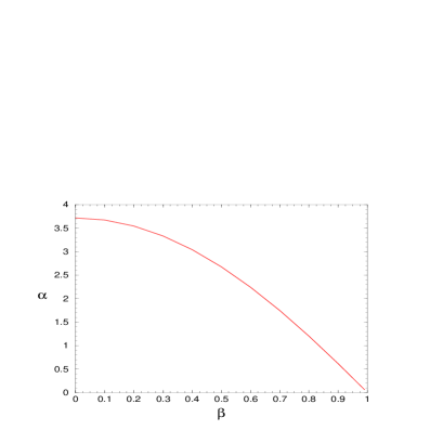
Figure 1: Function $\alpha(\beta)$ for LFD Yukawa model with $K_{11}$ channel only.

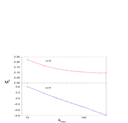
Figure 2: Cutoff dependence of the binding energy in the $J=0^{+}$ state ($\mu=0.25$), in the one-channel problem ($f_{1}$), for two fixed values of the coupling constant below and above the critical value.

Figure 2 shows the two different regimes, whether the coupling constant is below $(\alpha=3)$ or above $(\alpha=4)$ the critical value $\alpha_{c}$.

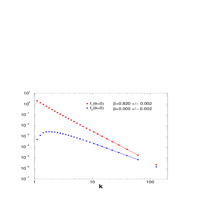
Figure 3: Asymptotical behavior of the $J=0^{+}$ wave function components $f_{i}$ for $B$=0.05, $\alpha$=1.096, $\mu$=0.25. The slope coefficient are $\beta_{1}=0.82$ and $\beta_{2}\approx 0$.

As it can be seen in Figure 3, the wave functions accurately follow the power law asymptotical behavior $1/k^{2+\beta}$ with a coefficient $\beta(\alpha)$ given in Figure 1. It is worth noticing that – at least in the framework of this model – one could measure the coupling constant from the asymptotic behavior of the bound state wave function.

A similar study has been done for the $J=1^{+}$ state, which is shown to be unstable without regularization [8, 9].

3 Pseudo-scalar coupling

The stability of the pseudo-scalar (PS) coupling is analyzed similarly to the scalar one. The same method leads to the conclusion that the equations for the PS coupling are quite surprisingly stable without any regularization.

However, the results show a ”quasi-degeneracy” of the coupling constant, for a wide range of binding energies. One has for instance (see Figure 4) $\alpha=49.5$ for a system with $B=0.001$, and $\alpha=48.6$ for a system five hundred times more deeply bound ($B=0.5$), that is only a 2% difference.

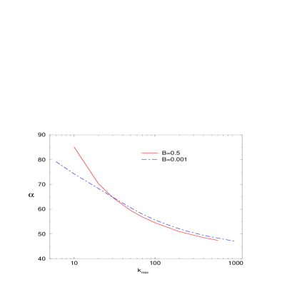
Figure 4: Convergence of coupling constants as function of the cutoff $k_{max}$ for $B=0.001$ and $B=0.5$. The exchange mass is $\mu=0.15$.

This peculiar behavior can be shown to come from the second channel:

$$[M^{2}-4(k^{2}+m^{2})]f_{2}(k,\theta)=$$

$${m^{2}\over 2\pi^{3}}\int K^{PS}_{22}(k,k^{\prime},\theta,\theta^{\prime},M^{2})f_{2}(k^{\prime},\theta^{\prime}){d^{3}k^{\prime}\over\varepsilon_{k^{\prime}}}$$ (7)

The kernel $K_{22}(k,k^{\prime},\theta,\theta^{\prime},M^{2})$, whose expression is explicitly given in [3], is represented in Figure 5 for fixed values of $\theta,\theta^{\prime}$. It vanishes for $k=0$ or $k^{\prime}=0$ and tends towards a positive constant in all the $(k,k^{\prime})$ plane.

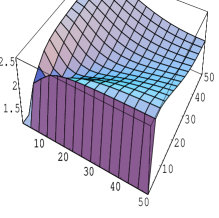
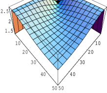
Figure 5: $K_{22}$ kernel in $(k,k^{\prime})$ plane.

Let us modelize this kernel by a kind of ”potential barrier” in the momentum space ($k,k^{\prime}$), displayed in Figure 6, whose advantage is to be analytically solvable.

Figure 6: Modelization of $K_{22}$ by a simpler kernel in the $(k,k^{\prime})$ plane.

$$K(k,k^{\prime})={\alpha U_{1}\over m^{2}}\Theta(k^{\prime}-k_{1})\Theta(k_{2}-k^{\prime})$$

$$\times \left[\Theta(k-k_{1})\Theta(k_{2}-k)+\Theta(k-k_{2})\Theta(k_{max}-k)\right]$$

$$+ \Theta(k^{\prime}-k_{2})\Theta(k_{max}-k^{\prime})\left[{\alpha U_{1}\over m^{2}}\Theta(k-k_{1})\right.$$

$$\times \left.\Theta(k_{2}-k)+{\alpha U_{2}\over m^{2}}\Theta(k-k_{2})\Theta(k_{max}-k)\right]$$

with $\Theta(x)=1,\,x>0$ and $\Theta(x)=0,\;x\leq 0$. This kernel has the same characteristics than $K^{PS}_{22}$ since it is zero when $k,k^{\prime}\to 0$,and tends towards a constant when $(k,k^{\prime})$ go to infinity with a fixed ratio $\gamma=k^{\prime}/k$.

$f_{2}$ satisfies the Schrödinger type equation

$$[k^{2}+\kappa^{2}]f_{2}(k)=-{m^{2}\over(2\pi)^{3}}\int K(k,k^{\prime})f_{2}(k^{\prime}){d^{3}k^{\prime}\over k^{\prime}}$$ (8)

with $\kappa^{2}=m^{2}-{M^{2}\over 4}$. We assume that $k_{1}<k_{2}<k_{max}$ et $U_{2}<U_{1}$. The term $\varepsilon_{k^{\prime}}$ in the volume element of (3) was replaced by its large momentum behavior, that is by $k^{\prime}$. We define $\Gamma(k)=[k^{2}+\kappa^{2}]f_{2}(k)$. The equation for $\Gamma(k)$, which is analytically solvable, reads:

$$\Gamma(k)=-{m^{2}\over 2\pi^{2}}\int_{-\infty}^{+\infty}K(k,k^{\prime}){\Gamma(k^{\prime})\over k^{\prime 2}+\kappa^{2}}k^{\prime}dk^{\prime}$$

The solution $\Gamma(k)$ is constant for $k_{1}<k<k_{2}$ and $k_{2}<k<k_{max}$ :

$$\Gamma(k) = \Gamma_{1}\Theta(k-k_{1})\Theta(k_{2}-k)$$

$$+ \Gamma_{2}\Theta(k-k_{2})\Theta(k_{max}-k)$$

The $\Gamma_{i}$ satisfy the coupled equations

$$\left\{\begin{array}[]{ccc}(1+\alpha u_{1}a)\;\Gamma_{1}&=&-\alpha u_{1}b\Gamma_{2}\\ (1+\alpha u_{2}b)\;\Gamma_{2}&=&-\alpha u_{1}a\Gamma_{1}\end{array}\right.$$

where we have defined $u_{i}={m^{2}\over 2\pi^{2}}U_{i}$ and

$$a=\log\left(k_{2}^{2}+\kappa^{2}\over k_{1}^{2}+\kappa^{2}\right),\quad b=\log\left(k_{max}^{2}+\kappa^{2}\over k_{2}^{2}+\kappa^{2}\right)$$ (10)

Replacing $\Gamma(k)$ by its definition in terms of $f_{2}(k)$, we finally get the solution of equation (8) on the form:

$$f_{2}(k) = {N\over k^{2}+\kappa^{2}}\left[\Theta(k-k_{1})\Theta(k_{2}-k)\right.$$

$$- \left.{\alpha au_{1}\over(1+\alpha bu_{2})}\Theta(k-k_{2})\Theta(k_{max}-k)\right]$$

where $N$ is a normalisation constant. For a given $\kappa$ the coupling constant is

$$\alpha(\kappa)={(au_{1}+bu_{2})+\sqrt{(au_{1}-bu_{2})^{2}+4u_{1}^{2}ab}\over 2abu_{1}(u_{1}-u_{2})}$$

and the results provided by this simple kernel are summarized in Table 1.

Table 1: Coupling constant as a function of the binding energy for the analytical model of the PS coupling second channel.

$$\begin{array}[]{||c|c||}\hline\cr B&\alpha\\ \hline\cr 0.001&22.5327\\ \hline\cr 0.010&22.5334\\ \hline\cr 0.100&22.5396\\ \hline\cr 0.500&22.5639\\ \hline\cr 1,00&22.5862\\ \hline\cr 1.50&22.5995\\ \hline\cr 2.00&22.6040\\ \hline\cr\end{array}$$

$\alpha(\kappa)$ depends on $\kappa$ through logarithms in $a,b$, eq. (10). Besides, the value of $\kappa$ is much smaller than $k_{1},k_{2},k_{max}$. This explains the very weak dependence of $\alpha(\kappa)$ v.s. $\kappa$.

We conclude from the above discussion that, even if the PS coupling does not formally need any regularization to insure its stability, calculations without form factors – though analytically understood – lead to results which are hardly interpretable on the physical point of vue.

Acknowledgements: The numerical calculations were performed at CGCV (CEA Grenoble) and IDRIS (CNRS). We are grateful to the staff members of these two organizations for their constant support.