Exploring N=1 SYM(2+1): the Stress-Tensor Correlator

Abstract

The evaluation of field theoretic correlators at strong couplings is especially interesting in the light of recently discovered string/field theory correspondences. We present a calculation of the stress-tensor correlator in ${\cal N}=1$ SYM theory in 2+1 dimensions. We calculate this object numerically with the method of supersymmetric discrete light-cone quantization (SDLCQ) at large $N_{c}$. For small distances we reproduce the conformal field theory result with the correlator behaving like $1/r^{6}$. In the large $r$ limit the correlator is determined by the (massless) BPS states of the theory. We find a critical value of the coupling where the correlator goes to zero in this limit. This critical coupling is shown to grow linearly with the square root of the transverse momentum resolution.

1 Introduction

In the present note we will report on the evaluation of the correlator of the stress-energy tensor in three-dimensional ${\cal N}=1$ supersymmetric Yang-Mills theory (SYM(2+1)). Correlation functions play a crucial role in string/field theory correspondences, because they can typically be calculated both on the string and on the field theory side. The crucial difficulty is that due to the nature of the correspondence, the correlator has to be evaluated in the strong coupling regime on one of the sides. In the past, we have used the non-perturbative method of supersymmetric discrete light-cone quantization (SDLCQ) to evaluate correlators at strong couplings, with encouraging results for the validity of the conjectured correspondence [1].

While ${\cal N}=1$ SYM(2+1) is interesting by itself for a number of reasons, it is the version of this theory with extended ${\cal N}=8$ supersymmetry that corresponds to a string theory of D2 branes [5]. We have learned from past calculations that the number of supersymmetry operators greatly enhances the size of the numerical calculations. As a first step towards the full ${\cal N}=8$ calculations we tackle ${\cal N}=1$ SYM(2+1) here.

Contrary to the mass spectrum, correlators use all spectral information, namely energy eigenvalues and the eigenfunctions, and can thus be used to test wavefunctions. In the present case, this is especially useful in order to examine the BPS states of the theory. These states are annihilated by one of the supercharges, and their masses are protected by their symmetry properties, whereas their wavefunctions could change as a function of the coupling. This is what we seem to find in the present study.

From conformal field theory it is known that the behavior of the correlator as a function of the distance $r$ between the operators should be like $1/r^{6}$ for small distances. On the other hand, the contributions of bound states will have a characteristic length scale associated with their size and one would therefore expect a $1/r^{5}$ behavior at small $r$. The different contributions have thus to work in concert to give the correct $1/r^{6}$ behavior. We will reproduce this behavior both analytically by calculating the free particle correlator and numerically by evaluating the correlator in the interacting theory. At large distances we find a critical coupling where the correlator goes to zero. In general we find a good convergence in both the longitudinal and the transverse cutoffs, which is non-trivial since we are dealing here with a three-dimensional theory, whereas most of our previous studies were in 1+1 dimensions. From conformal field theory calculations one knows that the correlators are simpler in collinear limit $x_{\perp}\rightarrow 0$, and we will work in this limit.

2 SDLCQ of N=1 SYM(2+1)

Discretized light-cone quantization (DLCQ) can be formulated in a way that preserves supersymmetry at each step of calculation [2]. Namely, one discretizes the supercharge $Q^{-}$ rather than the Hamiltonian $P^{-}$. This special approach is called supersymmetric DLCQ, or SDLCQ. One uses light-cone coordinates

$$x^{\pm}\equiv\frac{1}{\sqrt{2}}(x^{0}\pm x^{1}),\qquad x^{\perp} = x^{\perp},$$

where $X^{+}$ plays the role of a time. The total longitudinal momentum is denoted by $P^{+}$, $P^{-}$ is the light-cone energy, and $P^{\perp}$ the total transverse momentum.

Let us now focus on ${\cal N}=1$ SYM(2+1). The action is

$$S=\int d^{2}x\int_{0}^{l}dx_{\perp}\mbox{tr}(-\frac{1}{4}F^{\mu\nu}F_{\mu\nu}+{\rm i}{\bar{\Psi}}\gamma^{\mu}D_{\mu}\Psi).$$

We decompose the spinor $\Psi$ in terms of its projections, $(\psi,\chi)$, and use the light-cone gauge, $A^{+}=0$. The advantage of this physical gauge is that we can express everything in terms of the physical degrees of freedom, which are in the present example the fields $\psi$ and $\phi\equiv A^{\perp}$. The light-cone supercharge is a two-component Majorana spinor, and is decomposed into the projections

$$Q^{+} = 2^{1/4}\int dx^{-}\int_{0}^{l}dx_{\perp}\mbox{tr}\left[\phi\partial_{-}\psi-\psi\partial_{-}\phi\right],$$

$$Q^{-} = 2^{3/4}\int dx^{-}\int_{0}^{l}dx_{\perp}\mbox{tr}\left[2\partial_{\perp}\phi\psi\right.$$ (1)

$$\left.+g_{\rm YM}\left({\rm i}[\phi,\partial_{-}\phi]+2\psi\psi\right)\frac{1}{\partial_{-}}\psi\right].$$

One can explicitly check that the supersymmetry algebra is fulfilled

$$\{Q^{\pm},Q^{\pm}\}=2\sqrt{2}P^{\pm},\quad\{Q^{+},Q^{-}\}=-4P_{\perp}.$$ (2)

In DLCQ one discretizes the theory by compactifying $x^{-}$ on circle of period $2L=2\pi K/P^{+}$, with the harmonic resolution $K$, which is a cutoff in particle number. In the transverse direction, one compactifies $x^{\perp}$ on circle of period $l$, with a transverse cutoff $\pm 2\pi T/l$. The periodic boundary condition for the fields dictated by the supersymmetric formulation. The momentum modes become discrete and we can use the standard Fourier expansion for the fields $\phi$ and $\psi$. With the usual commutation relations the supercharges become

$$Q^{+} = {\rm i}2^{1/4}\sum_{n^{\perp}\in{\bf Z}}\int_{0}^{\infty}\sqrt{k}\left[b_{ij}^{\dagger}(k,n^{\perp})a_{ij}(k,n^{\perp})\right.$$

$$\left.\qquad\qquad\quad-a_{ij}^{\dagger}(k,n^{\perp})b_{ij}(k,n^{\perp})\right]dk,$$

$$Q^{-} {=} Q^{-}_{1}+g_{\rm YM}Q^{-}_{2}.$$

The exact expressions for $Q^{-}_{1,2}$ are listed in Ref. [4]. Here it suffices to note that $Q^{-}$ is linear in the coupling $g_{\rm YM}$. We want to calculate the spectrum of the theory on the computer, and need therefore finite dimensional representations of these operators. They are obtained by applying a truncation procedure, which defines the (finite) Fock basis. The longitudinal momentum of a particle can take the values $n_{i}=0,1,2...,K$, and the transverse components are $n^{\perp}_{i}=0,\pm 1,\pm 2,...,\pm T$. This symmetric truncation ensures the conservation of transverse parity symmetry, which leads to exactly degenerate doublets. The other symmetry of the theory is the so-called S-Symmetry, which is non-degenerate and is related to the orientation of the string of partons in the Fock state; it results in a sign change when the color indices of an operator are flipped. Additionally we have supersymmetry, so we get a total factor of 8 savings in linear matrix size and the density of eigenstates will be much smaller, which allows for a better interpretation of results.

The program is then to construct the supercharge $Q^{-}$, apply Eq. (2) to calculate the Hamiltonian $P^{-}$ by squaring $Q^{-}$, and to diagonalize $P^{-}$ to obtain eigenvalues and -functions. These data go into the calculation of the correlator, which we describe in the next section. We retrieve the continuum results by solving the system for lager and larger $K$, reaching the continuum limit $K\rightarrow\infty$ eventually by extrapolation.

3 Correlation functions

The general expression for a correlator in light-cone formulation is

$$F(x^{+},x^{-},x^{\perp})=$$

$$\qquad\langle 0|T^{++}(x^{+},x^{-},x^{\perp})T^{++}(0,0,0)|0\rangle.$$ (3)

Inspired by the simpler structure of correlators in the collinear limit $x^{\perp}=0$ in conformal field theory, we apply the same limit here. We can evaluate the expression, Eq. (3), by inserting a complete set $|\alpha\rangle$ with energy eigenvalues $P^{-}_{\alpha}$

$$F(x^{+},x^{-},x^{\perp}=0)=$$

$$\qquad\sum_{\alpha}\langle 0|T^{++}(x^{-},0,x^{\perp}=0)|\alpha\rangle$$

$$\qquad\qquad\qquad\times e^{-iP^{-}_{\alpha}x^{+}}\langle\alpha|T^{++}(0,0,0)|0\rangle.$$

The momentum operator is

$$T^{++}(x) = {\rm tr}\left[(\partial_{-}\phi)^{2}+{1\over 2}\left(i\psi\partial_{-}\psi-i(\partial_{-}\psi)\psi\right)\right]$$

$$= T^{++}_{B}(x)+T^{++}_{F}(x)\,.$$

Its boson and fermion contributions expressed in mode operators are

$$\frac{L}{\pi}T^{++}_{B}(n,m)|0\rangle={\sqrt{nm}\over 2}a^{\dagger}_{ij}(n)a^{\dagger}_{ji}(m)|0\rangle$$ (4)

$$\frac{L}{\pi}T^{++}_{F}(n,m)|0\rangle={(n-m)\over 4}b^{\dagger}_{ij}(n)b^{\dagger}_{ji}(m)|0\rangle\,.$$ (5)

The important thing to notice here is that only the two-particle states contribute to these operators.

3.1 Free case

It is instructive to consider the free case, because we know from conformal field theory that we should obtain a $1/r^{6}$ behavior. The eigenfunctions $|\alpha\rangle$ are now a set of free particles with mass $m$. The four independent sums over quantum numbers are converted to integrals by

$$\frac{1}{L}\sum_{n}\rightarrow\frac{1}{\pi}\int dk\quad\mbox{and}\quad\frac{1}{l}\sum_{n_{\perp}}\rightarrow\frac{1}{2\pi}\int dk_{\perp}.$$

The evaluation of the bosonic contribution, Eq. (4), yields

$$F(x^{+},x^{-},0)_{B}=\frac{i}{2(2\pi)^{3}}m^{5}\left(\frac{x^{+}}{x^{-}}\right)^{2}\frac{1}{x}K^{2}_{5/2}(mx)\,,$$

where $x^{2}=2x^{-}x^{+}$. Analogously we can evaluate the fermion contribution, Eq. (5), and get

$$F(x^{+},x^{-},0)_{F}=\frac{i}{4(2\pi)^{3}}m^{5}\left(\frac{x^{+}}{x^{-}}\right)^{2}\frac{1}{x}$$

$$\qquad\times\left[K_{7/2}(mx)K_{3/2}(mx)-K^{2}_{5/2}(mx)\right]\,.$$ (6)

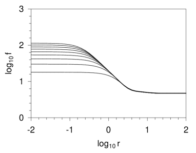
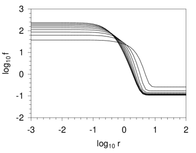
Figure 1: The log-log plot of the correlation function $f\equiv r^{5}\langle T^{++}(x)T^{++}(0)\rangle\left({x^{-}\over x^{+}}\right)^{2}\frac{16\pi^{3}}{105}{{K^{3}l}\over\sqrt{-i}}$ vs. $r$ (a) for $g{=}0.10$ at $K{=}4$ [top]; (b) for $g{=}1$ at $K=5$ [bottom]. The transverse cutoff runs from $T=1$ to 9.

We continue to Euclidean space by taking $r=\sqrt{2x^{+}x^{-}}$ to be real. In the small-$r$ limit we recover the $1/r^{6}$ behavior

$$\left(\frac{x^{-}}{x^{+}}\right)^{2}F(x^{+},x^{-},0)=\frac{-3i}{8(2\pi)^{2}}\frac{1}{r^{6}}\,,$$

expected from conformal field theory.

3.2 Full bound-state correlator

In the full calculation we use the bound-state solutions obtained from SDLCQ and insert them into the expression for the correlator. It is useful to write

$$F(x^{+},x^{-},0)=\sum_{n,m,s,t}\,\,\left(\frac{\pi}{2L^{2}l}\right)^{2}$$

$$\!\!\!\!\!\!\!\!\!\!\!\!\times\langle 0|\frac{L}{\pi}T^{++}(n,m)e^{-iP^{-}_{op}x^{+}-iP^{+}x^{-}}\frac{L}{\pi}T^{++}(s,t)|0\rangle\,,$$

and to use the notation

$$\frac{1}{N_{u}}|u\rangle=\frac{L}{\pi}\sum_{n,m}\delta^{n+m}_{K}\delta^{n_{\perp}+m_{\perp}}_{N_{\perp}}T^{++}(n,m)|0\rangle,$$

with a normalization factor $N_{u}$. We insert the complete set of bound-states $|\alpha\rangle$ with masses $M_{\alpha}$. After some algebra to separate the dependencies on the different length scales in the problem we obtain

$$F(x^{+},x^{-},0) = \frac{1}{2\pi}\sum_{K,N_{\perp},\alpha}\frac{1}{2L}\frac{1}{l}\left(\frac{\pi K}{L}\right)^{3}$$

$$\!\!\!\!\!\!\times e^{-iP^{-}_{\alpha}x^{+}-iP^{+}x^{-}}\left[\frac{|\langle u|\alpha\rangle|^{2}}{lK^{3}|N_{u}|^{2}}\right]\,.$$

Evaluation of sums over $K$ and $N_{\perp}$ as integrals yields finally

$$\!\!\!\!\!\!\frac{1}{\sqrt{-i}}\left(\frac{x^{-}}{x^{+}}\right)^{2}F(x^{+},x^{-},0)=$$ (8)

$$\sum_{\alpha}\frac{1}{2(2\pi)^{5/2}}\frac{M_{\alpha}^{9/2}}{\sqrt{r}}K_{9/2}(M_{\alpha}r)\left[\frac{|\langle u|\alpha\rangle|^{2}}{lK^{3}|N_{u}|^{2}}\right]$$

The term in square brackets is basically the overlap of the bound state $|\alpha\rangle$ with the vector $|u\rangle\propto T^{++}|0\rangle$. It is calculated numerically and multiplied by some function of the distance $r$ involving the Bessel function $K_{9/2}$. It is clear from Eq. (8) that we need both the eigenfunctions $|\alpha\rangle$ and the mass eigenvalues $M_{\alpha}$ to evaluate this expression.

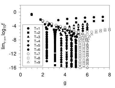
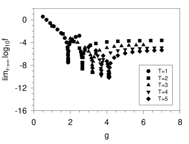
Figure 2: The large-$r$ limit of $f\equiv r^{5}\langle T^{++}(x)T^{++}(0)\rangle\left({x^{-}\over x^{+}}\right)^{2}\frac{16\pi^{3}}{105}{{K^{3}l}\over\sqrt{-i}}$ vs. $g$ for (a) $K=5$ [top]; (b) $K=6$ [bottom].

For free particles we have two independent sums over the transverse momenta, and would therefore expect that the transverse dimension be controlled by the dimensional scale of the bound state $R_{B}$. Hence, the correlation function should scale like $1/r^{4}R_{B}^{2}$. Because of transverse boost invariance, however, the matrix element are independent of the difference of transverse momenta, and scales like $1/r^{5}R_{B}$.

4 Numerical Results

At small distances $r$, we expect the correlator to behave like $1/r^{6}$, because at large energies the bound states will look like free particles. Eq. (8) on the other hand tells us that each individual bound state behaves like $1/r^{5}$. We have to have a coherent behavior of all states to get the $1/r^{6}$ behavior, and this is a non-trivial check of our results. Looking at Fig. 1, we observe exactly this behavior. The constant $1/r^{5}$ behavior of the curves at very small distances is caused by numerical artifacts, basically because the largest possible mass in the system is regulated by the transverse cutoff and is not infinite. The slope of minus unity around $r=0$ gives rise to the correct $1/r^{6}$ behavior. It consistently sets in at smaller $r$ for larger cutoffs $K$ and $T$.

At large $r$ the correlator is totally determined by the massless states. Actually, there are two types of massless states. The massless states at $g=0$ are reflections of all the states of the dimensionally reduced theory in $1+1$ [3][4]. They behave as $g^{2}M^{2}_{1+1}$, and for $g\simeq 0$ there should be no dependence of the correlator on the transverse momentum cutoff $T$ at large $r$. This is exactly what we find in our calculations, see Fig. 1. Secondly, we have states that are exactly massless for all $g$, which are the BPS states. They are actually massless at all resolutions, but have a complicated dependence on the coupling $g$ through their wavefunctions. In this way the correlator gives us information on wavefunctions of the BPS states.

Surprisingly, we also find a coupling dependence of the large-$r$ limit of the correlator, see Fig. 2. Correlator does not change monotonically with $g$, but has singularity at a ’critical’ coupling which is a function of $K$ and $T$. If we plot the ‘critical’ couplings vs. $\sqrt{T}$ in Fig. 3, we find that the coupling is a linear function of $\sqrt{T}$ at $K=5$ and 6. So we would conclude that ‘critical’ coupling goes to infinity in the transverse continuum limit.

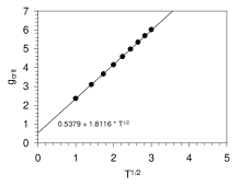
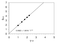
Figure 3: Critical coupling $g_{\rm crit}$ versus $\sqrt{T}$ for (a) $K=5$ and (b) $K=6$.

Unfortunately, we see no region dominated by massive bound states, where $r$ is large enough to see structure of the bound states but small enough that the correlator is not dominated by massless states.

5 Conclusions

We presented the first calculation of the correlator of the stress-energy tensor from first principles in three-dimensional ${\cal N}=1$ SYM. We recovered the $1/r^{6}$ behavior of the free particle correlator, also known from conformal field theory. The individual $1/r^{5}$ behaviors of the bound states add up to give this result which is a non-trivial test of our results. At large $r$ we found that the BPS states depend on the coupling through their wavefunctions, altough their masses stay fixed due to their symmetry properties. We found a vanishing correlator at some ’critical’ coupling $g_{crit}\propto\sqrt{T}$, which seems to be a numerical artifact of the discrete approach. Some remarks on the computer code seem in order. The present code handles two million Fock states, and uses all known symmetries in the problem(SUSY, parity, S-symmetry), which in turn gives a factor eight of reduction in the matrix size to be diagonalized. Calculations in 3+1 dimensions seem therefore not completely out of reach. Another challenge is the evaluation of the correlator in the ${\cal N}=(8,8)$ version of SYM(2+1). This theory is conjectured to correspond to a string theory of D2-branes. We hope to report on progress in this direction soon, which would establish a further test of a version of the Maldacena conjecture.

References

- [1] F. Antonuccio, O. Lunin, S. Pinsky, and A. Hashimoto, JHEP 07 (1999) 029; J.R. Hiller, O. Lunin, S. Pinsky, U. Trittmann, Phys. Lett. B482 (2000) 409.
- [2] Y. Matsumura, N. Sakai, and T. Sakai, Phys. Rev. D52 (1995) 2446.
- [3] F. Antonuccio, O. Lunin, and S. Pinsky, Phys. Rev. D58 (1998) 085009.
- [4] F. Antonuccio, O. Lunin, and S. Pinsky, Phys. Rev. D59 (1999) 085001; P. Haney, J.R. Hiller, O. Lunin, S. Pinsky, and U. Trittmann, Phys. Rev. D62 (2000) 075002.
- [5] N. Itzhaki, J. M. Maldacena, J. Sonnenschein and S. Yankielowicz, Phys. Rev. D 58, 046004 (1998).