226E 226F

CENTRE DE PHYSIQUE THÉORIQUE

CNRS - Luminy, Case 907

13288 Marseille Cedex 9

FORCES FROM CONNES’ GEOMETRY

Thomas SCHÜCKER

Abstract

We try to give a pedagogical introduction to Connes’ derivation of the standard model of electro-magnetic, weak and strong forces from gravity.

Lectures given at the Autumn School “Topology and Geometry in Physics”
of the Graduiertenkolleg ‘Physical Systems with Many Degrees of Freedom’
Universität Heidelberg
September 2001, Rot an der Rot, Germany
Editors: Eike Bick & Frank Steffen
Lecture Notes in Physics 659, Springer, 2005

PACS-92: 11.15 Gauge field theories
MSC-91: 81T13 Yang-Mills and other gauge theories

CPT-01/P.4264
hep-th/0111236

1 Introduction

Still today one of the major summits in physics is the understanding of the spectrum of the hydrogen atom. The phenomenological formula by Balmer and Rydberg was a remarkable pre-summit on the way up. The true summit was reached by deriving this formula from quantum mechanics. We would like to compare the standard model of electro-magnetic, weak, and strong forces with the Balmer-Rydberg formula [1] and review the present status of Connes’ derivation of this model from noncommutative geometry, see table 1. This geometry extends Riemannian geometry, and Connes’ derivation is a natural extension of another major summit in physics: Einstein’s derivation of general relativity from Riemannian geometry. Indeed, Connes’ derivation unifies gravity with the other three forces.

atoms	particles and forces
Balmer-Rydberg formula	standard model
quantum mechanics	noncommutative geometry

Table 1: An analogy

Let us briefly recall four nested, analytic geometries and their impact on our understanding of forces and time, see table 2. Euclidean geometry is underlying Newton’s mechanics as space of positions. Forces are described by vectors living in the same space and the Euclidean scalar product is needed to define work and potential energy. Time is not part of geometry, it is absolute. This point of view is abandoned in special relativity unifying space and time into Minkowskian geometry. This new point of view allows to derive the magnetic field from the electric field as a pseudo force associated to a Lorentz boost. Although time has become relative, one can still imagine a grid of synchronized clocks, i.e. a universal time. The next generalization is Riemannian geometry = curved spacetime. Here gravity can be viewed as the pseudo force associated to a uniformly accelerated coordinate transformation. At the same time, universal time loses all meaning and we must content ourselves with proper time. With today’s precision in time measurement, this complication of life becomes a bare necessity, e.g. the global positioning system (GPS).

geometry	force	time
Euclidean	$E=\int\vec{F}\cdot\hbox{\rm d}\vec{x}$	absolute
Minkowskian	$\vec{E},\epsilon_{0}\Rightarrow\vec{B},\mu_{0}=\,\frac{1}{\epsilon_{0}c^{2}}\,$	universal
Riemannian	Coriolis $\leftrightarrow$ gravity	proper, $\tau$
noncommutative	gravity $\Rightarrow$ YMH, $\lambda={\textstyle\frac{1}{3}}g_{2}^{2}$	$\Delta\tau\sim 10^{-40}$ s

Table 2: Four nested analytic geometries

Our last generalization is to Connes’ noncommutative geometry = curved space(time) with uncertainty. It allows to understand some Yang-Mills and some Higgs forces as pseudo forces associated to transformations that extend the two coordinate transformations above to the new geometry without points. Also, proper time comes with an uncertainty. This uncertainty of some hundred Planck times might be accessible to experiments through gravitational wave detectors within the next ten years [2].

Prerequisites

On the physical side, the reader is supposed to be acquainted with general relativity, e.g. [3], Dirac spinors at the level of e.g. the first few chapters in [4] and Yang-Mills theory with spontaneous symmetry break-down, for example the standard model, e.g. [5]. I am not ashamed to adhere to the minimax principle: a maximum of pleasure with a minimum of effort. The effort is to do a calculation, the pleasure is when its result coincides with an experiment result. Consequently our mathematical treatment is as low-tech as possible. We do need local differential and Riemannian geometry at the level of e.g. the first few chapters in [6]. Local means that our spaces or manifolds can be thought of as open subsets of ${\mathbb{R}}^{4}$. Nevertheless, we sometimes use compact spaces like the torus: only to simplify some integrals. We do need some group theory, e.g. [7], mostly matrix groups and their representations. We also need a few basic facts on associative algebras. Most of them are recalled as we go along and can be found for instance in [8]. For the reader’s convenience, a few simple definitions from groups and algebras are collected in the appendix. And, of course, we need some chapters of noncommutative geometry which are developped in the text. For a more detailed presentation still with particular care for the physicist see [9, 10].

2 Gravity from Riemannian geometry

In this section, we briefly review Einstein’s derivation of general relativity from Riemannian geometry. His derivation is in two strokes, kinematics and dynamics.

2.1 First stroke: kinematics

Consider flat space(time) $M$ in inertial or Cartesian coordinates $\tilde{x}^{\tilde{\lambda}}$. Take as matter a free, classical point particle. Its dynamics, Newton’s free equation, fixes the trajectory $\tilde{x}^{\tilde{\lambda}}(p)$:

$${\frac{\hbox{\rm d}^{2}\tilde{x}^{\tilde{\lambda}}}{\hbox{\rm d}p^{2}}}\,=0.$$ (1)

After a general coordinate transformation, $x^{\lambda}=\sigma^{\lambda}(\tilde{x})$, Newton’s equation reads

$${\,\frac{\hbox{\rm d}^{2}x^{\lambda}}{\hbox{\rm d}p^{2}}\,}+\hbox{$\Gamma^{\lambda}$}_{\mu\nu}(g){\,\frac{\hbox{\rm d}x^{\mu}}{\hbox{\rm d}p}\,}{\,\frac{\hbox{\rm d}x^{\nu}}{\hbox{\rm d}p}\,}=0.$$ (2)

Pseudo forces have appeared. They are coded in the Levi-Civita connection

$$\hbox{$\Gamma^{\lambda}$}_{\mu\nu}(g)={\textstyle\frac{1}{2}}g^{\lambda\kappa}\left[\,\frac{{\partial}}{{\partial}x^{\mu}}\,g_{\kappa\nu}+\,\frac{{\partial}}{{\partial}x^{\nu}}\,g_{\kappa\mu}-\,\frac{{\partial}}{{\partial}x^{\kappa}}\,g_{\mu\nu}\right],$$ (3)

where $g_{\mu\nu}$ is obtained by ‘fluctuating’ the flat metric $\tilde{\eta}_{\tilde{\mu}\tilde{\nu}}={\rm diag}(1,-1,-1,-1,)$ with the Jacobian of the coordinate transformation $\sigma$:

$$g_{\mu\nu}(x)={{\cal J}(x)^{-1\tilde{\mu}}}_{\mu}\,\eta_{\tilde{\mu}\tilde{\nu}}\,{{\cal J}(x)^{-1\tilde{\nu}}}_{\nu},\quad{{\cal J}(\tilde{x})^{\mu}}_{\tilde{\mu}}:={\partial}\sigma^{\mu}(\tilde{x})/{\partial}\ \tilde{x}^{\tilde{\mu}}.$$ (4)

For the coordinates of the rotating disk, the pseudo forces are precisely the centrifugal and Coriolis forces. Einstein takes uniformly accelerated coordinates, $ct=c\tilde{t},\ z=\tilde{z}+{\textstyle\frac{1}{2}}{\textstyle\frac{g}{c^{2}}}(c\tilde{t})^{2}$ with $g=9.81\ \rm m/s^{2}$. Then the geodesic equation (2) reduces to $\hbox{\rm d}^{2}z/\hbox{\rm d}t^{2}=-g$. So far this gravity is still a pseudo force which means that the curvature of its Levi-Civita connection vanishes. This constraint is relaxed by the equivalence principle: pseudo forces and true gravitational forces are coded together in a not necessarily flat connection $\Gamma$, that derives from a potential, the not necessarily flat metric $g$. The kinematical variable to describe gravity is therefore the Riemannian metric. By construction the dynamics of matter, the geodesic equation, is now covariant under general coordinate transformations.

2.2 Second stroke: dynamics

Now that we know the kinematics of gravity let us see how Einstein obtains its dynamics, i.e. differential equations for the metric tensor $g_{\mu\nu}$. Of course Einstein wants these equations to be covariant under general coordinate transformations and he wants the energy-momentum tensor $T_{\mu\nu}$ to be the source of gravity. From Riemannian geometry he knew that there is no covariant, first order differential operator for the metric. But there are second order ones:
Theorem: The most general tensor of degree 2 that can be constructed from the metric tensor $g_{\mu\nu}(x)$ with at most two partial derivatives is

$$\alpha R_{\mu\nu}+\beta Rg_{\mu\nu}+\Lambda g_{\mu\nu},\quad\alpha,\ \beta,\ \Lambda\in{\mathbb{R}}..$$ (5)

Here are our conventions for the curvature tensors:

$${\rm Riemann\ tensor:} {R^{\lambda}}_{\mu\nu\kappa}={\partial}_{\nu}{\Gamma^{\lambda}}_{\mu\kappa}-{\partial}_{\kappa}{\Gamma^{\lambda}}_{\mu\nu}+{\Gamma^{\eta}}_{\mu\kappa}{\Gamma^{\lambda}}_{\nu\eta}-{\Gamma^{\eta}}_{\mu\nu}{\Gamma^{\lambda}}_{\kappa\eta},$$ (6)

$${\rm Ricci\ tensor:} R_{\mu\kappa}={R^{\lambda}}_{\mu\lambda\kappa},$$ (7)

$${\rm curvature\ scalar:} R=R_{\mu\nu}g^{\mu\nu}.$$ (8)

The miracle is that the tensor (5) is symmetric just as the energy-momentum tensor. However, the latter is covariantly conserved, $\hbox{\rm D}^{\mu}T_{\mu\nu}=0$, while the former one is conserved if and only if $\beta=-{\textstyle\frac{1}{2}}\alpha$. Consequently, Einstein puts his equation

$$R_{\mu\nu}-{\textstyle\frac{1}{2}}Rg_{\mu\nu}-\Lambda_{c}g_{\mu\nu}={\textstyle\frac{8\pi G}{c^{4}}}\,T_{\mu\nu}.$$ (9)

He chooses a vanishing cosmological constant, $\Lambda_{c}=0$. Then for small static mass density $T_{00}$, his equation reproduces Newton’s universal law of gravity with $G$ the Newton constant. However for not so small masses there are corrections to Newton’s law like precession of perihelia. Also Einstein’s theory applies to massless matter and produces the curvature of light. Einstein’s equation has an agreeable formal property, it derives via the Euler-Lagrange variational principle from an action, the famous Einstein-Hilbert action:

$$S_{EH}[g]=\frac{-1}{16\pi G}\,\int_{M}R\,\hbox{\rm d}V\ -\,\frac{2\Lambda_{c}}{16\pi G}\,\int_{M}\hbox{\rm d}V,$$ (10)

with the invariant volume element $\hbox{\rm d}V:=|\det g_{\cdot\cdot}|^{1/2}\,\hbox{\rm d}^{4}x.$

General relativity has a precise geometric origin: the left-hand side of Einstein’s equation is a sum of some $80\,000$ terms in first and second partial derivatives of $g_{\mu\nu}$ and its matrix inverse $g^{\mu\nu}$. All of these terms are completely fixed by the requirement of covariance under general coordinate transformations. General relativity is verified experimentally to an extraordinary accuracy, even more, it has become a cornerstone of today’s technology. Indeed length measurements had to be abandoned in favour of proper time measurements, e.g. the GPS. Nevertheless, the theory still leaves a few questions unanswered:

• Einstein’s equation is nonlinear and therefore does not allow point masses as source, in contrast to Maxwell’s equation that does allow point charges as source. From this point of view it is not satisfying to consider point-like matter.

• The gravitational force is coded in the connection $\Gamma$. Nevertheless we have accepted its potential, the metric $g$, as kinematical variable.

• The equivalence principle states that locally, i.e. on the trajectory of a point-like particle, one cannot distinguish gravity from a pseudo force. In other words, there is always a coordinate system, ‘the freely falling lift’, in which gravity is absent. This is not true for electro-magnetism and we would like to derive this force (as well as the weak and strong forces) as a pseudo force coming from a geometric transformation.

• So far general relativity has resisted all attempts to reconcile it with quantum mechanics.

3 Slot machines and the standard model

Today we have a very precise phenomenological description of electro-magnetic, weak, and strong forces. This description, the standard model, works on a perturbative quantum level and, as classical gravity, it derives from an action principle. Let us introduce this action by analogy with the Balmer-Rydberg formula.

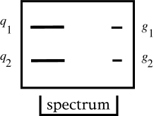
Figure 1: A slot machine for atomic spectra

One of the new features of atomic physics was the appearance of discrete frequencies and the measurement of atomic spectra became a highly developed art. It was natural to label the discrete frequencies $\nu$ by natural numbers $n$. To fit the spectrum of a given atom, say hydrogen, let us try the ansatz

$$\nu=g_{1}n_{1}^{q_{1}}+g_{2}n_{2}^{q_{2}}.$$ (11)

We view this ansatz as a slot machine. You input two bills, the integers $q_{1}$, $q_{2}$ and two coins, the two real numbers $g_{1}$, $g_{2}$, and compare the output with the measured spectrum. (See Figure 1.) If you are rich enough, you play and replay on the slot machine until you win. The winner is the Balmer-Rydberg formula, i.e., $q_{1}=q_{2}=-2$ and $g_{1}=-g_{2}=\ 3.289\ 10^{15}$ Hz, which is the famous Rydberg constant $R$. Then came quantum mechanics. It explained why the spectrum of the hydrogen atom was discrete in the first place and derived the exponents and the Rydberg constant,

$$R=\,\frac{m_{e}}{4\pi\hbar^{3}}\,\frac{e^{4}}{(4\pi\epsilon_{0})^{2}}\,,$$ (12)

from a noncommutativity, $[x,p]=i\hbar 1$.

To cut short its long and complicated history we introduce the standard model as the winner of a particular slot machine. This machine, which has become popular under the names Yang, Mills and Higgs, has four slots for four bills. Once you have decided which bills you choose and entered them, a certain number of small slots will open for coins. Their number depends on the choice of bills. You make your choice of coins, feed them in, and the machine starts working. It produces as output a Lagrange density. From this density, perturbative quantum field theory allows you to compute a complete particle phenomenology: the particle spectrum with the particles’ quantum numbers, cross sections, life times, and branching ratios. (See Figure 2.) You compare the phenomenology to experiment to find out whether your input wins or loses.

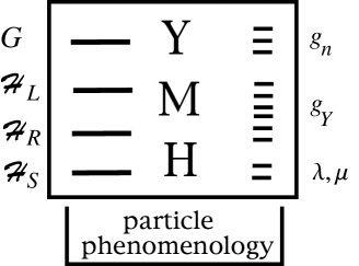
Figure 2: The Yang-Mills-Higgs slot machine

3.1 Input

The first bill is a finite dimensional, real, compact Lie group $G$. The gauge bosons, spin 1, will live in its adjoint representation whose Hilbert space is the complexification of the Lie algebra ${\mathfrak{g}}$ (cf Appendix).

The remaining bills are three unitary representations of $G$, $\rho_{L},\ \rho_{R},\ \rho_{S}$, defined on the complex Hilbert spaces, ${\cal H}_{L},\ {\cal H}_{R},\ {\cal H}_{S}$. They classify the left- and right-handed fermions, spin ${\textstyle\frac{1}{2}}$, and the scalars, spin 0. The group $G$ is chosen compact to ensure that the unitary representations are finite dimensional, we want a finite number of ‘elementary particles’ according to the credo of particle physics that particles are orthonormal basis vectors of the Hilbert spaces which carry the representations. More generally, we might also admit multi-valued representations, ‘spin representations’, which would open the debate on charge quantization. More on this later.

The coins are numbers, coupling constants, more precisely coefficients of invariant polynomials. We need an invariant scalar product on ${\mathfrak{g}}$. The set of all these scalar products is a cone and the gauge couplings are particular coordinates of this cone. If the group is simple, say $G=SU(n)$, then the most general, invariant scalar product is

$$(X,X^{\prime})={\textstyle\frac{2}{g_{n}^{2}}}{\rm tr}\,[X^{*}X^{\prime}],\quad X,X^{\prime}\in su(n).$$ (13)

If $G=U(1)$, we have

$$(Y,Y^{\prime})={\textstyle\frac{1}{g_{1}^{2}}}\bar{Y}Y^{\prime},\quad Y,Y^{\prime}\in u(1).$$ (14)

We denote by $\bar{\cdot}$ the complex conjugate and by $\cdot^{*}$ the Hermitean conjugate. Mind the different normalizations, they are conventional. The $g_{n}$ are positive numbers, the gauge couplings. For every simple factor of $G$ there is one gauge coupling.

Then we need the Higgs potential $V(\varphi)$. It is an invariant, fourth order, stable polynomial on ${\cal H}_{S}\owns\varphi$. Invariant means $V(\rho_{S}(u)\varphi)=V(\varphi)$ for all $u\in G$. Stable means bounded from below. For $G=U(2)$ and the Higgs scalar in the fundamental or defining representation, $\varphi\in{\cal H}_{S}={\mathbb{C}}^{2}$, $\rho_{S}(u)=u$, we have

$$V(\varphi)=\lambda\,(\varphi^{*}\varphi)^{2}-{\textstyle\frac{1}{2}}\mu^{2}\,\varphi^{*}\varphi.$$ (15)

The coefficients of the Higgs potential are the Higgs couplings, $\lambda$ must be positive for stability. We say that the potential breaks $G$ spontaneously if no minimum of the potential is a trivial orbit under $G$. In our example, if $\mu$ is positive, the minima of $V(\varphi)$ lie on the 3-sphere $|\varphi|=v:={\textstyle\frac{1}{2}}\mu/\sqrt{\lambda}$. $v$ is called vacuum expectation value and $U(2)$ is said to break down spontaneously to its little group

$$U(1)\owns\pmatrix{1&0\cr 0&e^{i\alpha}}.$$ (16)

The little group leaves invariant any given point of the minimum, e.g. $\varphi=(v,0)^{T}$. On the other hand, if $\mu$ is purely imaginary, then the minimum of the potential is the origin, no spontaneous symmetry breaking and the little group is all of $G$.

Finally, we need the Yukawa couplings $g_{Y}$. They are the coefficients of the most general, real, trilinear invariant on ${\cal H}_{L}^{*}\,\otimes\,{\cal H}_{R}\,\otimes\,({\cal H}_{S}\oplus{\cal H}_{S}^{*})$. For every 1-dimensional invariant subspace in the reduction of this tensor representation, we have one complex Yukawa coupling. For example $G=U(2)$, ${\cal H}_{L}={\mathbb{C}}^{2}$, $\rho_{L}(u)\psi_{L}=(\det u)^{q_{L}}u\,\psi_{L},$ ${\cal H}_{R}={\mathbb{C}}$, $\rho_{R}(u)\psi_{R}=(\det u)^{q_{R}}\psi_{R},$ ${\cal H}_{S}={\mathbb{C}}^{2}$, $\rho_{S}(u)\varphi=(\det u)^{q_{S}}u\,\varphi$. If $-q_{L}+q_{R}+q_{S}\not=0$ there is no Yukawa coupling, otherwise there is one: $(\psi_{L},\psi_{R},\varphi)={\rm Re}(g_{Y}\,\psi_{L}^{*}\psi_{R}\varphi)$.

If the symmetry is broken spontaneously, gauge and Higgs bosons acquire masses related to gauge and Higgs couplings, fermions acquire masses equal to the ‘vacuum expectation value’ $v$ times the Yukawa couplings.

As explained in Jan-Willem van Holten’s and Jean Zinn-Justin’s lectures at this School [11, 12], one must require for consistency of the quantum theory that the fermionic representations be free of Yang-Mills anomalies,

$${\rm tr}\,((\tilde{\rho}_{L}(X))^{3})-{\rm tr}\,((\tilde{\rho}_{R}(X))^{3})=0,\quad{\rm for\ all}\ X\in{\mathfrak{g}}.$$ (17)

We denote by $\tilde{\rho}$ the Lie algebra representation of the group representation $\rho$. Sometimes one also wants the mixed Yang-Mills-gravitational anomalies to vanish:

$${\rm tr}\,\tilde{\rho}_{L}(X)-{\rm tr}\,\tilde{\rho}_{R}(X)=0,\quad{\rm for\ all}\ X\in{\mathfrak{g}}.$$ (18)

3.2 Rules

It is time to open the slot machine and to see how it works. Its mechanism has five pieces:

The Yang-Mills action: The actor in this piece is $A=A_{\mu}\hbox{\rm d}x^{\mu}$, called connection, gauge potential, gauge boson or Yang-Mills field. It is a 1-form on spacetime $M\owns x$ with values in the Lie algebra ${\mathfrak{g}}$, $A\in\Omega^{1}(M,{\mathfrak{g}}).$ We define its curvature or field strength,

$$F:=\hbox{\rm d}A+{\textstyle\frac{1}{2}}[A,A]={\textstyle\frac{1}{2}}F_{\mu\nu}\hbox{\rm d}x^{\mu}\hbox{\rm d}x^{\nu}\ \in\Omega^{2}(M,{\mathfrak{g}}),$$ (19)

and the Yang-Mills action,

$$S_{YM}[A]=-{\textstyle\frac{1}{2}}\int_{M}(F,*F)=\,\frac{-1}{2g_{n}^{2}}\,\int_{M}{\rm tr}\,F^{*}_{\mu\nu}F^{\mu\nu}\hbox{\rm d}V.$$ (20)

The gauge group ${}^{M}G$ is the infinite dimensional group of differentiable functions $g:M\rightarrow G$ with pointwise multiplication. $\cdot^{*}$ is the Hermitean conjugate of matrices, $*\cdot$ is the Hodge star of differential forms. The space of all connections carries an affine representation (cf Appendix) $\rho_{V}$ of the gauge group:

$$\rho_{V}(g)A=gAg^{-1}+g\hbox{\rm d}g^{-1}.$$ (21)

Restricted to $x$-independent (‘rigid’) gauge transformation, the representation is linear, the adjoint one. The field strength transforms homogeneously even under $x$-dependent (‘local’) gauge transformations, $g:M\rightarrow G$ differentiable,

$$\rho_{V}(g)F=gFg^{-1},$$ (22)

and, as the scalar product $(\cdot,\cdot)$ is invariant, the Yang-Mills action is gauge invariant,

$$S_{YM}[\rho_{V}(g)A]=S_{YM}[A]\quad{\rm for\ all}\ g\in\ ^{M}G.$$ (23)

Note that a mass term for the gauge bosons,

$${\textstyle\frac{1}{2}}\int_{M}m^{2}_{A}(A,*A)=\,\frac{1}{g_{n}^{2}}\,\int_{M}m^{2}_{A}{\rm tr}\,A_{\mu}^{*}A^{\mu}\hbox{\rm d}V,$$ (24)

is not gauge invariant because of the inhomogeneous term in the transformation law of a connection (21). Gauge invariance forces the gauge bosons to be massless.

In the Abelian case $G=U(1)$, the Yang-Mills Lagrangian is nothing but Maxwell’s Lagrangian, the gauge boson $A$ is the photon and its coupling constant $g$ is $e/\sqrt{\epsilon_{0}}$. Note however, that the Lie algebra of $U(1)$ is $i{\mathbb{R}}$ and the vector potential is purely imaginary, while conventionally, in Maxwell’s theory it is chosen real. Its quantum version is $QED$, quantum electro-dynamics. For $G=SU(3)$ and ${\cal H}_{L}={\cal H}_{R}={\mathbb{C}}^{3}$ we have today’s theory of strong interaction, quantum chromo-dynamics, $QCD$.

The Dirac action: Schrödinger’s action is non-relativistic. Dirac generalized it to be Lorentz invariant, e.g. [4]. The price to be paid is twofold. His generalization only works for spin ${\textstyle\frac{1}{2}}$ particles and requires that for every such particle there must be an antiparticle with same mass and opposite charges. Therefore, Dirac’s wave function $\psi(x)$ takes values in ${\mathbb{C}}^{4}$, spin up, spin down, particle, antiparticle. Antiparticles have been discovered and Dirac’s theory was celebrated. Here it is in short for (flat) Minkowski space of signature $+---$, $\eta_{\mu\nu}=\eta^{\mu\nu}={\rm diag}(+1,-1,-1,-1)$. Define the four Dirac matrices,

$$\gamma^{0}=\pmatrix{0&-1_{2}\cr-1_{2}&0},\quad\gamma^{j}=\pmatrix{0&\sigma_{j}\cr-\sigma_{j}&0},$$ (25)

for $j=1,2,3$ with the three Pauli matrices,

$$\sigma_{1}=\pmatrix{0&1\cr 1&0},\quad\sigma_{2}=\pmatrix{0&-i\cr i&0},\quad\sigma_{3}=\pmatrix{1&0\cr 0&-1}.$$ (26)

They satisfy the anticommutation relations,

$$\gamma^{\mu}\gamma^{\nu}+\gamma^{\nu}\gamma^{\mu}=2\eta^{\mu\nu}1_{4}.$$ (27)

In even spacetime dimensions, the chirality,

$$\gamma_{5}:=-{\textstyle\frac{i}{4!}}\epsilon_{\mu\nu\rho\sigma}\gamma^{\mu}\gamma^{\nu}\gamma^{\rho}\gamma^{\sigma}=-i\gamma^{0}\gamma^{1}\gamma^{2}\gamma^{3}=\pmatrix{-1_{2}&0\cr 0&1_{2}}$$ (28)

is a natural operator and it paves the way to an understanding of parity violation in weak interactions. The chirality is a unitary matrix of unit square, which anticommutes with all four Dirac matrices. $(1-\gamma_{5})/2$ projects a Dirac spinor onto its left-handed part, $(1+\gamma_{5})/2$ projects onto the right-handed part. The two parts are called Weyl spinors. A massless left-handed (right-handed) spinor, has its spin parallel (anti-parallel) to its direction of propagation. The chirality maps a left-handed spinor to a right-handed spinor. A space reflection or parity transformation changes the sign of the velocity vector and leaves the spin vector unchanged. It therefore has the same effect on Weyl spinors as the chirality operator. Similarly, there is the charge conjugation, an anti-unitary operator (cf Appendix) of unit square, that applied on a particle $\psi$ produces its antiparticle

$$J={\textstyle\frac{1}{i}}\gamma^{2}\circ\,{\rm complex\ conjugation}=\pmatrix{0&0&0&-1\cr 0&0&1&0\cr 0&1&0&0\cr-1&0&0&0}\,\circ\,{\rm c\ c},$$ (29)

i.e. $J\psi={\textstyle\frac{1}{i}}\gamma^{2}\ \bar{\psi}$. Attention, here and for the last time $\bar{\psi}$ stands for the complex conjugate of $\psi$. In a few lines we will adopt a different more popular convention. The charge conjugation commutes with all four Dirac matrices times $i$. In flat spacetime, the free Dirac operator is simply defined by,

$${\,\hbox{$\partial\!\!\!/$}}:=i\hbar\gamma^{\mu}{\partial}_{\mu}.$$ (30)

It is sometimes referred to as square root of the wave operator because ${\,\hbox{$\partial\!\!\!/$}}^{2}=-\,\hbox{$\sqcap\!\!\!\!\sqcup$}$. The coupling of the Dirac spinor to the gauge potential $A=A_{\mu}\hbox{\rm d}x^{\mu}$ is done via the covariant derivative, and called minimal coupling. In order to break parity, we write left- and right-handed parts independently:

$$S_{D}[A,\psi_{L},\psi_{R}] = \int_{M}\bar{\psi}_{L}\left[{\,\hbox{$\partial\!\!\!/$}}+i\hbar\gamma^{\mu}\tilde{\rho}_{L}(A_{\mu})\right]\,\frac{1-\gamma_{5}}{2}\,\psi_{L}\,\hbox{\rm d}V$$ (32)

$$+\int_{M}\bar{\psi}_{R}\left[{\,\hbox{$\partial\!\!\!/$}}+i\hbar\gamma^{\mu}\tilde{\rho}_{R}(A_{\mu})\right]\,\frac{1+\gamma_{5}}{2}\,\psi_{R}\,\hbox{\rm d}V.$$

The new actors in this piece are $\psi_{L}$ and $\psi_{R}$, two multiplets of Dirac spinors or fermions, that is with values in ${\cal H}_{L}$ and ${\cal H}_{R}$. We use the notations, $\bar{\psi}:=\psi^{*}\gamma^{0}$, where $\cdot^{*}$ denotes the Hermitean conjugate with respect to the four spinor components and the dual with respect to the scalar product in the (internal) Hilbert space ${\cal H}_{L}$ or ${\cal H}_{R}$. The $\gamma^{0}$ is needed for energy reasons and for invariance of the pseudo–scalar product of spinors under lifted Lorentz transformations. The $\gamma^{0}$ is absent if spacetime is Euclidean. Then we have a genuine scalar product and the square integrable spinors form a Hilbert space ${\cal L}^{2}({\cal S})={\cal L}^{2}({\mathbb{R}}^{4})\otimes{\mathbb{C}}^{4}$, the infinite dimensional brother of the internal one. The Dirac operator is then self adjoint in this Hilbert space. We denote by $\tilde{\rho}_{L}$ the Lie algebra representation in ${\cal H}_{L}$. The covariant derivative, $\hbox{\rm D}_{\mu}:={\partial}_{\mu}+\tilde{\rho}_{L}(A_{\mu})$, deserves its name,

$$\left[{\partial}_{\mu}+\tilde{\rho}_{L}(\rho_{V}(g)A_{\mu})\right](\rho_{L}(g)\psi_{L})=\rho_{L}(g)\left[{\partial}_{\mu}+\tilde{\rho}_{L}(A_{\mu})\right]\psi_{L},$$ (33)

for all gauge transformations $g\in\,^{M}\!G$. This ensures that the Dirac action (32) is gauge invariant.

If parity is conserved, ${\cal H}_{L}={\cal H}_{R}$, we may add a mass term

$$-c\int_{M}\bar{\psi}_{R}\,m_{\psi}\,\frac{1-\gamma_{5}}{2}\,\psi_{L}\,\hbox{\rm d}V\ -\ c\int_{M}\bar{\psi}_{L}\,m_{\psi}\,\frac{1+\gamma_{5}}{2}\,\psi_{R}\,\hbox{\rm d}V\ =\ -c\int_{M}\bar{\psi}\,m_{\psi}\,\psi\,\hbox{\rm d}V$$ (34)

to the Dirac action. It gives identical masses to all members of the multiplet. The fermion masses are gauge invariant if all fermions in ${\cal H}_{L}={\cal H}_{R}$ have the same mass. For instance $QED$ preserves parity, ${\cal H}_{L}={\cal H}_{R}={\mathbb{C}}$, the representation being characterized by the electric charge, $-1$ for both the left- and right handed electron. Remember that gauge invariance forces gauge bosons to be massless. For fermions, it is parity non-invariance that forces them to be massless.

Let us conclude by reviewing briefly why the Dirac equation is the Lorentz invariant generalization of the Schrödinger equation. Take the free Schrödinger equation on (flat) ${\mathbb{R}}^{4}$. It is a linear differential equation with constant coefficients,

$$\left(\,\frac{2m}{i\hbar}\,\frac{{\partial}}{{\partial}t}\,-\Delta\right)\psi=0.$$ (35)

We compute its polynomial following Fourier and de Broglie,

$$-\,\frac{2m}{\hbar}\,\omega+k^{2}=-\,\frac{2m}{\hbar^{2}}\,\left[E-\,\frac{p^{2}}{2m}\,\right].$$ (36)

Energy conservation in Newtonian mechanics is equivalent to the vanishing of the polynomial. Likewise, the polynomial of the free, massive Dirac equation $({\,\hbox{$\partial\!\!\!/$}}-cm_{\psi})\psi=0$ is

$${\textstyle\frac{\hbar}{c}}\,\omega\gamma^{0}+\hbar\,k_{j}\gamma^{j}-c\,m1.$$ (37)

Putting it to zero implies energy conservation in special relativity,

$$({\textstyle\frac{\hbar}{c}})^{2}\,\omega^{2}-\hbar^{2}\,\vec{k}^{2}-c^{2}\,m^{2}=0.$$ (38)

In this sense, Dirac’s equation generalizes Schrödinger’s to special relativity. To see that Dirac’s equation is really Lorentz invariant we must lift the Lorentz transformations to the space of spinors. We will come back to this lift.

So far we have seen the two noble pieces by Yang-Mills and Dirac. The remaining three pieces are cheap copies of the two noble ones with the gauge boson $A$ replaced by a scalar $\varphi$. We need these three pieces to cure only one problem, give masses to some gauge bosons and to some fermions. These masses are forbidden by gauge invariance and parity violation. To simplify the notation we will work from now on in units with $c=\hbar=1$.

The Klein-Gordon action: The Yang-Mills action contains the kinetic term for the gauge boson. This is simply the quadratic term, $(\hbox{\rm d}A,\hbox{\rm d}A)$, which by Euler-Lagrange produces linear field equations. We copy this for our new actor, a multiplet of scalar fields or Higgs bosons,

$$\varphi\in\Omega^{0}(M,{\cal H}_{S}),$$ (39)

by writing the Klein-Gordon action,

$$S_{KG}[A,\varphi]={\textstyle\frac{1}{2}}\int_{M}(\hbox{\rm D}\varphi)^{*}*\hbox{\rm D}\varphi={\textstyle\frac{1}{2}}\int_{M}(\hbox{\rm D}_{\mu}\varphi)^{*}\hbox{\rm D}^{\mu}\varphi\,\hbox{\rm d}V,$$ (40)

with the covariant derivative here defined with respect to the scalar representation,

$$\hbox{\rm D}\varphi:=\hbox{\rm d}\varphi+\tilde{\rho}_{S}(A)\varphi.$$ (41)

Again we need this minimal coupling $\varphi^{*}A\varphi$ for gauge invariance.

The Higgs potential: The non-Abelian Yang-Mills action contains interaction terms for the gauge bosons, an invariant, fourth order polynomial, $2(\hbox{\rm d}A,[A,A])+([A,A],[A,A])$. We mimic these interactions for scalar bosons by adding the integrated Higgs potential $\int_{M}*V(\varphi)$ to the action.

The Yukawa terms: We also mimic the (minimal) coupling of the gauge boson to the fermions $\psi^{*}A\psi$ by writing all possible trilinear invariants,

$$S_{Y}[\psi_{L},\psi_{R},\varphi]:={\rm Re}\int_{M}*\left(\sum_{j=1}^{n}g_{Yj}\left(\psi_{L}^{*},\psi_{R},\varphi\right)_{j}+\sum_{j=n+1}^{m}g_{Yj}\left(\psi_{L}^{*},\psi_{R},\varphi^{*}\right)_{j}\right).$$ (42)

In the standard model, there are 27 complex Yukawa couplings, $m=27$.

The Yang-Mills and Dirac actions, contain three types of couplings, a trilinear self coupling $AAA$, a quadrilinear self coupling $AAAA$ and the trilinear minimal coupling $\psi^{*}A\psi$. The gauge self couplings are absent if the group $G$ is Abelian, the photon has no electric charge, Maxwell’s equations are linear. The beauty of gauge invariance is that if $G$ is simple, all these couplings are fixed in terms of one positive number, the gauge coupling $g$. To see this, take an orthonormal basis $T_{b},\ b=1,2,...\dim G$ of the complexification ${\mathfrak{g}}^{\mathbb{C}}$ of the Lie algebra with respect to the invariant scalar product and an orthonormal basis $F_{k},\ k=1,2,...\dim{\cal H}_{L}$, of the fermionic Hilbert space, say ${\cal H}_{L}$, and expand the actors,

$$A=:A_{\mu}^{b}T_{b}\hbox{\rm d}x^{\mu},\quad\psi=:\psi^{k}F_{k}.$$ (43)

Insert these expressions into the Yang-Mills and Dirac actions, then you get the following interaction terms, see Figure 3,

$$g\,{\partial}_{\rho}A_{\mu}^{a}A_{\nu}^{b}A_{\sigma}^{c}\,f_{abc}\,\epsilon^{\rho\mu\nu\sigma},\quad g^{2}\,A_{\mu}^{a}A_{\nu}^{b}A_{\rho}^{c}A_{\sigma}^{d}\,{f_{ab}}^{e}{f_{ecd}}\,\epsilon^{\rho\mu\nu\sigma},\quad g\,\psi^{k*}A^{b}_{\mu}\gamma^{\mu}\psi_{\ell}\,{{t_{b}}_{k}}^{\ell},$$ (44)

with the structure constants ${f_{ab}}^{e}$,

$$[T_{a},T_{b}]=:{f_{ab}}^{e}T_{e}.$$ (45)

The indices of the structure constants are raised and lowered with the matrix of the invariant scalar product in the basis $T_{b}$, that is the identity matrix. The ${{t_{b}}_{k}}^{\ell}$ is the matrix of the operator $\tilde{\rho}_{L}(T_{b})$ with respect to the basis $F_{k}$. The difference between the noble and the cheap actions is that the Higgs couplings, $\lambda$ and $\mu$ in the standard model, and the Yukawa couplings $g_{Yj}$ are arbitrary, are neither connected among themselves nor connected to the gauge couplings $g_{i}$.

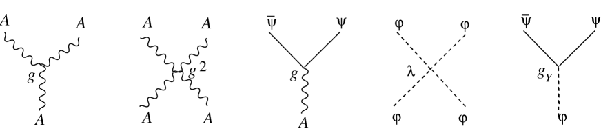
Figure 3: Tri- and quadrilinear gauge couplings, minimal gauge coupling to fermions, Higgs selfcoupling and Yukawa coupling

3.3 The winner

Physicists have spent some thirty years and billions of Swiss Francs playing on the slot machine by Yang, Mills and Higgs. There is a winner, the standard model of electro-weak and strong forces. Its bills are

$$G = SU(2)\times U(1)\times SU(3)/({\mathbb{Z}}_{2}\times{\mathbb{Z}}_{3}),$$ (46)

$${\cal H}_{L} = \bigoplus_{1}^{3}\left[(2,{\textstyle\frac{1}{6}},3)\oplus(2,-{\textstyle\frac{1}{2}},1)\right],$$ (48)

$${\cal H}_{R} = \bigoplus_{1}^{3}\left[(1,{\textstyle\frac{2}{3}},3)\oplus(1,-{\textstyle\frac{1}{3}},3)\oplus(1,-1,1)\right],$$ (49)

$${\cal H}_{S} = (2,-{\textstyle\frac{1}{2}},1),$$ (50)

where $(n_{2},y,n_{3})$ denotes the tensor product of an $n_{2}$ dimensional representation of $SU(2)$, an $n_{3}$ dimensional representation of $SU(3)$ and the one dimensional representation of $U(1)$ with hypercharge $y$: $\rho(\exp(i\theta))=\exp(iy\theta)$. For historical reasons the hypercharge is an integer multiple of ${\textstyle\frac{1}{6}}$. This is irrelevant: only the product of the hypercharge with its gauge coupling is measurable and we do not need multi-valued representations, which are characterized by non-integer, rational hypercharges. In the direct sum, we recognize the three generations of fermions, the quarks are $SU(3)$ colour triplets, the leptons colour singlets. The basis of the fermion representation space is

$$\pmatrix{u\cr d}_{L},\ \pmatrix{c\cr s}_{L},\ \pmatrix{t\cr b}_{L},\ \pmatrix{\nu_{e}\cr e}_{L},\ \pmatrix{\nu_{\mu}\cr\mu}_{L},\ \pmatrix{\nu_{\tau}\cr\tau}_{L}$$

$$\matrix{u_{R},\cr d_{R},}\quad\matrix{c_{R},\cr s_{R},}\quad\matrix{t_{R},\cr b_{R},}\quad e_{R},\quad\mu_{R},\quad\tau_{R}$$

The parentheses indicate isospin doublets.

The eight gauge bosons associated to $su(3)$ are called gluons. Attention, the $U(1)$ is not the one of electric charge, it is called hypercharge, the electric charge is a linear combination of hypercharge and weak isospin, parameterized by the weak mixing angle $\theta_{w}$ to be introduced below. This mixing is necessary to give electric charges to the $W$ bosons. The $W^{+}$ and $W^{-}$ are pure isospin states, while the $Z^{0}$ and the photon are (orthogonal) mixtures of the third isospin generator and hypercharge.

Because of the high degree of reducibility in the bills, there are many coins, among them 27 complex Yukawa couplings. Not all Yukawa couplings have a physical meaning and we only remain with 18 physically significant, positive numbers [13], three gauge couplings at energies corresponding to the $Z$ mass,

$$g_{1}=0.3574\pm 0.0001, g_{2}=0.6518\pm 0.0003, g_{3}=1.218\pm 0.01,$$ (51)

two Higgs couplings, $\lambda$ and $\mu$, and 13 positive parameters from the Yukawa couplings. The Higgs couplings are related to the boson masses:

$$m_{W} = {\textstyle\frac{1}{2}}g_{2}\,v\,=\,80.419\pm 0.056\ {\rm GeV},$$ (52)

$$m_{Z} = {\textstyle\frac{1}{2}}\sqrt{g_{1}^{2}+g_{2}^{2}}\ v=m_{W}/\cos\theta_{w}\,=\,91.1882\,\pm\,0.0022\ {\rm GeV},$$ (53)

$$m_{H} = 2\sqrt{2}\sqrt{\lambda}\,v\,>\,98\ {\rm GeV},$$ (54)

with the vacuum expectation value $v:={\textstyle\frac{1}{2}}\mu/\sqrt{\lambda}$ and the weak mixing angle $\theta_{w}$ defined by

$$\sin^{2}\theta_{w}:=g_{2}^{-2}/(g_{2}^{-2}+g_{1}^{-2})=0.23117\,\pm\,0.00016.$$ (55)

For the standard model, there is a one–to–one correspondence between the physically relevant part of the Yukawa couplings and the fermion masses and mixings,

$$m_{e}=0.510998902\pm 0.000000021\ {\rm MeV}, m_{u}=3\pm 2\ {\rm MeV}, m_{d}=6\pm 3\ {\rm MeV},$$ (56)

$$m_{\mu}=0.105658357\pm 0.000000005\ {\rm GeV}, m_{c}=1.25\pm 0.1\ {\rm GeV}, m_{s}=0.125\pm 0.05\ {\rm GeV},$$ (57)

$$m_{\tau}=1.77703\pm 0.00003\ {\rm GeV}, m_{t}=174.3\pm 5.1\ {\rm GeV}, m_{b}=4.2\pm 0.2\ {\rm GeV}.$$

For simplicity, we take massless neutrinos. Then mixing only occurs for quarks and is given by a unitary matrix, the Cabibbo-Kobayashi-Maskawa matrix

$$C_{KM}:=\pmatrix{V_{ud}&V_{us}&V_{ub}\cr V_{cd}&V_{cs}&V_{cb}\cr V_{td}&V_{ts}&V_{tb}}.$$ (58)

For physical purposes it can be parameterized by three angles $\theta_{12}$, $\theta_{23}$, $\theta_{13}$ and one $CP$ violating phase $\delta$:

$$C_{KM}=\pmatrix{c_{12}c_{13}&s_{12}c_{13}&s_{13}e^{-i\delta}\cr-s_{12}c_{23}-c_{12}s_{23}s_{13}e^{i\delta}&c_{12}c_{23}-s_{12}s_{23}s_{13}e^{i\delta}&s_{23}c_{13}\cr s_{12}s_{23}-c_{12}c_{23}s_{13}e^{i\delta}&-c_{12}s_{23}-s_{12}c_{23}s_{13}e^{i\delta}&c_{23}c_{13}},$$ (59)

with $c_{kl}:=\cos\theta_{kl}$, $s_{kl}:=\sin\theta_{kl}$. The absolute values of the matrix elements in $C_{KM}$ are:

$$\pmatrix{0.9750\pm 0.0008&0.223\pm 0.004&0.004\pm 0.002\cr 0.222\pm 0.003&0.9742\pm 0.0008&0.040\pm 0.003\cr 0.009\pm 0.005&0.039\pm 0.004&0.9992\pm 0.0003}.$$ (60)

The physical meaning of the quark mixings is the following: when a sufficiently energetic $W^{+}$ decays into a $u$ quark, this $u$ quark is produced together with a $\bar{d}$ quark with probability $|V_{ud}|^{2}$, together with a $\bar{s}$ quark with probability $|V_{us}|^{2}$, together with a $\bar{b}$ quark with probability $|V_{ub}|^{2}$. The fermion masses and mixings together are an entity, the fermionic mass matrix or the matrix of Yukawa couplings multiplied by the vacuum expectation value.

Let us note six intriguing properties of the standard model.

• The gluons couple in the same way to left- and right-handed fermions, the gluon coupling is vectorial, the strong interaction does not break parity.

• The fermionic mass matrix commutes with $SU(3)$, the three colours of a given quark have the same mass.

• The scalar is a colour singlet, the $SU(3)$ part of $G$ does not suffer spontaneous symmetry break down, the gluons remain massless.

• The $SU(2)$ couples only to left-handed fermions, its coupling is chiral, the weak interaction breaks parity maximally.

• The scalar is an isospin doublet, the $SU(2)$ part suffers spontaneous symmetry break down, the $W^{\pm}$ and the $Z^{0}$ are massive.

• The remaining colourless and neutral gauge boson, the photon, is massless and couples vectorially. This is certainly the most ad-hoc feature of the standard model. Indeed the photon is a linear combination of isospin, which couples only to left-handed fermions, and of a $U(1)$ generator, which may couple to both chiralities. Therefore only the careful fine tuning of the hypercharges in the three input representations (48-50) can save parity conservation and gauge invariance of electro-magnetism,

  $$y_{u_{R}}=y_{q_{L}}-y_{\ell_{L}}\quad y_{d_{R}}=y_{q_{L}}+y_{\ell_{L}},\quad y_{e_{R}}=2y_{\ell_{L}},\quad y_{\varphi}=y_{\ell_{L}},$$ (61)

  The subscripts label the multiplets, $qL$ for the left-handed quarks, $\ell L$ for the left-handed leptons, $uR$ for the right-handed up-quarks and so forth and $\varphi$ for the scalar.

Nevertheless the phenomenological success of the standard model is phenomenal: with only a handful of parameters, it reproduces correctly some millions of experimental numbers. Most of these numbers are measured with an accuracy of a few percent and they can be reproduced by classical field theory, no $\hbar$ needed. However, the experimental precision has become so good that quantum corrections cannot be ignored anymore. At this point it is important to note that the fermionic representations of the standard model are free of Yang-Mills (and mixed) anomalies. Today the standard model stands uncontradicted.

Let us come back to our analogy between the Balmer-Rydberg formula and the standard model. One might object that the ansatz for the spectrum, equation (11), is completely ad hoc, while the class of all (anomaly free) Yang-Mills-Higgs models is distinguished by perturbative renormalizability. This is true, but this property was proved [14] only years after the electro-weak part of the standard model was published [15].

By placing the hydrogen atom in an electric or magnetic field, we know experimentally that every frequency ‘state’ $n$, $n=1,2,3,...$, comes with $n$ irreducible unitary representations of the rotation group $SO(3)$. These representations are labelled by $\ell$, $\ell=0,1,2,...n-1$, of dimensions $2\ell+1$. An orthonormal basis of each representation $\ell$ is labelled by another integer $m$, $m=-\ell,-\ell+1,...\ell$. This experimental fact has motivated the credo that particles are orthonormal basis vectors of unitary representations of compact groups. This credo is also behind the standard model. While $SO(3)$ has a clear geometric interpretation, we are still looking for such an interpretation of $SU(2)\times U(1)\times SU(3)/[{\mathbb{Z}}_{2}\times{\mathbb{Z}}_{3}].$

We close this subsection with Iliopoulos’ joke [16] from 1976:

Do-it-yourself kit for gauge models:

1. Choose a gauge group $G$.

2. Choose the fields of the “elementary particles” you want to introduce, and their representations. Do not forget to include enough fields to allow for the Higgs mechanism.

3. Write the most general renormalizable Lagrangian invariant under $G$. At this stage gauge invariance is still exact and all vector bosons are massless.

4. Choose the parameters of the Higgs scalars so that spontaneous symmetry breaking occurs. In practice, this often means to choose a negative value [positive in our notations] for the parameter $\mu^{2}$.

5. Translate the scalars and rewrite the Lagrangian in terms of the translated fields. Choose a suitable gauge and quantize the theory.

6. Look at the properties of the resulting model. If it resembles physics, even remotely, publish it.

7. GO TO 1.

Meanwhile his joke has become experimental reality.

3.4 Wick rotation

Euclidean signature is technically easier to handle than Minkowskian. What is more, in Connes’ geometry it will be vital that the spinors form a Hilbert space with a true scalar product and that the Dirac action takes the form of a scalar product. We therefore put together the Einstein-Hilbert and Yang-Mills-Higgs actions with emphasis on the relative signs and indicate the changes necessary to pass from Minkowskian to Euclidean signature.

In 1983 the meter disappeared as fundamental unit of science and technology. The conceptual revolution of general relativity, the abandon of length in favour of time, had made its way up to the domain of technology. Said differently, general relativity is not really geo-metry, but chrono-metry. Hence our choice of Minkowskian signature is $+---$.

With this choice the combined Lagrangian reads,

$$\{-\,{\textstyle\frac{2\Lambda_{c}}{16\pi G}}\,-\,{\textstyle\frac{1}{16\pi G}}\,R\,-\,{\textstyle\frac{1}{2g^{2}}}{\rm tr}\,(F_{\mu\nu}^{*}F^{\mu\nu})\,+\,{\textstyle\frac{1}{g^{2}}}m_{A}^{2}{\rm tr}\,(A_{\mu}^{*}A^{\mu})$$ (62)

$$+\,{\textstyle\frac{1}{2}}\,(\hbox{\rm D}_{\mu}\varphi)^{*}\hbox{\rm D}^{\mu}\varphi\,-\,{\textstyle\frac{1}{2}}\,m_{\varphi}^{2}|\varphi|^{2}\,+\,{\textstyle\frac{1}{2}}\,\mu^{2}|\varphi|^{2}\,-\,\lambda|\varphi|^{4}$$ (63)

$$+\,\psi^{*}\gamma^{0}\,[i\gamma^{\mu}\hbox{\rm D}_{\mu}\,-\,m_{\psi}1_{4}]\,\psi\}\ |\!\det g_{\cdot\cdot}|^{1/2}.$$ (64)

This Lagrangian is real if we suppose that all fields vanish at infinity. The relative coefficients between kinetic terms and mass terms are chosen as to reproduce the correct energy momentum relations from the free field equations using Fourier transform and the de Broglie relations as explained after equation (35). With the chiral decomposition

$$\psi_{L} = {\textstyle\frac{1-\gamma_{5}}{2}}\,\psi,\quad\psi_{R}\ =\ {\textstyle\frac{1+\gamma_{5}}{2}}\,\psi,$$ (65)

the Dirac Lagrangian reads

$$\psi^{*}\gamma^{0}\,[i\gamma^{\mu}\hbox{\rm D}_{\mu}\,-\,m_{\psi}1_{4}]\,\psi$$ (66)

$$\quad=\psi_{L}^{*}\gamma^{0}\,i\gamma^{\mu}\hbox{\rm D}_{\mu}\,\psi_{L}\,+\,\psi_{R}^{*}\gamma^{0}\,i\gamma^{\mu}\hbox{\rm D}_{\mu}\,\psi_{R}\,-\,m_{\psi}\psi_{L}^{*}\gamma^{0}\psi_{R}\,-\,m_{\psi}\psi_{R}^{*}\gamma^{0}\psi_{L}.$$ (67)

The relativistic energy momentum relations are quadratic in the masses. Therefore the sign of the fermion mass $m_{\psi}$ is conventional and merely reflects the choice: who is particle and who is antiparticle. We can even adopt one choice for the left-handed fermions and the opposite choice for the right-handed fermions. Formally this can be seen by the change of field variable (chiral transformation):

$$\psi:=\exp(i\alpha\gamma_{5})\,\psi^{\prime}.$$ (68)

It leaves invariant the kinetic term and the mass term transforms as,

$$-m_{\psi}{\psi^{\prime}}^{*}\gamma^{0}[\cos(2\alpha)\,1_{4}+i\sin(2\alpha)\,\gamma_{5}]{\psi^{\prime}}.$$ (69)

With $\alpha=-\pi/4$ the Dirac Lagrangian becomes:

$${\psi^{\prime}}^{*}\gamma^{0}[\,i\gamma^{\mu}\hbox{\rm D}_{\mu}\,+im_{\psi}\gamma_{5}]{\psi}^{\prime}$$ (70)

$$\quad={\psi^{\prime}}_{L}^{*}\gamma^{0}\,i\gamma^{\mu}\hbox{\rm D}_{\mu}\,{\psi}^{\prime}_{L}\,+\,{\psi^{\prime}}_{R}^{*}\gamma^{0}\,i\gamma^{\mu}\hbox{\rm D}_{\mu}\,{\psi^{\prime}}_{R}\,+\,m_{\psi}{\psi^{\prime}}_{L}^{*}\gamma^{0}i\gamma_{5}{\psi^{\prime}}_{R}\,+\,m_{\psi}{\psi^{\prime}}_{R}^{*}\gamma^{0}i\gamma_{5}{\psi^{\prime}}_{L}$$ (71)

$$\quad={\psi^{\prime}}_{L}^{*}\gamma^{0}\,i\gamma^{\mu}\hbox{\rm D}_{\mu}\,{\psi}^{\prime}_{L}\,+\,{\psi^{\prime}}_{R}^{*}\gamma^{0}\,i\gamma^{\mu}\hbox{\rm D}_{\mu}\,{\psi^{\prime}}_{R}\,+\,im_{\psi}{\psi^{\prime}}_{L}^{*}\gamma^{0}{\psi^{\prime}}_{R}\,-\,im_{\psi}{\psi^{\prime}}_{R}^{*}\gamma^{0}{\psi^{\prime}}_{L}.$$ (72)

We have seen that gauge invariance forbids massive gauge bosons, $m_{A}=0$, and that parity violation forbids massive fermions, $m_{\psi}=0$. This is fixed by spontaneous symmetry breaking, where we take the scalar mass term with wrong sign, $m_{\varphi}=0,\ \mu>0$. The shift of the scalar then induces masses for the gauge bosons, the fermions and the physical scalars. These masses are calculable in terms of the gauge, Yukawa, and Higgs couplings.

The other relative signs in the combined Lagrangian are fixed by the requirement that the energy density of the non-gravitational part $T_{00}$ be positive (up to a cosmological constant) and that gravity in the Newtonian limit be attractive. In particular this implies that the Higgs potential must be bounded from below, $\lambda>0$. The sign of the Einstein-Hilbert action may also be obtained from an asymptotically flat space of weak curvature, where we can define gravitational energy density. Then the requirement is that the kinetic terms of all physical bosons, spin 0, 1, and 2, be of the same sign. Take the metric of the form

$$g_{\mu\nu}=\eta_{\mu\nu}+h_{\mu\nu},$$ (73)

$h_{\mu\nu}$ small. Then the Einstein-Hilbert Lagrangian becomes [17],

$$-\,{\textstyle\frac{1}{16\pi G}}\,R\,|\!\det g_{\cdot\cdot}|^{1/2} = {\textstyle\frac{1}{16\pi G}}\{{\textstyle\frac{1}{4}}{\partial}_{\mu}h_{\alpha\beta}{\partial}^{\mu}h^{\alpha\beta}\,-\,{\textstyle\frac{1}{8}}{\partial}_{\mu}{h_{\alpha}}^{\alpha}{\partial}^{\mu}{h_{\beta}}^{\beta}$$ (75)

$$-\,[{\partial}_{\nu}{h_{\mu}}^{\nu}-{\textstyle\frac{1}{2}}{\partial}_{\mu}{h_{\nu}}^{\nu}][{\partial}_{\nu^{\prime}}{h^{\mu}}^{\nu^{\prime}}-{\textstyle\frac{1}{2}}{\partial}^{\mu}{h_{\nu^{\prime}}}^{\nu^{\prime}}]\,+\,O(h^{3})\}.$$

Here indices are raised with $\eta^{\cdot\cdot}$. After an appropriate choice of coordinates, ‘harmonic coordinates’, the bracket $\left[{\partial}_{\nu}{h_{\mu}}^{\nu}-{\textstyle\frac{1}{2}}{\partial}_{\mu}{h_{\nu}}^{\nu}\right]$ vanishes and only two independent components of $h_{\mu\nu}$ remain, $h_{11}=-h_{22}$ and $h_{12}$. They represent the two physical states of the graviton, helicity $\pm 2$. Their kinetic terms are both positive, e.g.:

$$+{\textstyle\frac{1}{16\pi G}}{\textstyle\frac{1}{4}}{\partial}_{\mu}h_{12}{\partial}^{\mu}h_{12}.$$ (76)

Likewise, by an appropriate gauge transformation, we can achieve ${\partial}_{\mu}A^{\mu}=0$, ‘Lorentz gauge’, and remain with only two ‘transverse’ components $A_{1},\ A_{2}$ of helicity $\pm 1$. They have positive kinetic terms, e.g.:

$$+{\textstyle\frac{1}{2g^{2}}}{\rm tr}\,({\partial}_{\mu}A_{1}^{*}{\partial}^{\mu}A_{1}).$$ (77)

Finally, the kinetic term of the scalar is positive:

$$+{\textstyle\frac{1}{2}}{\partial}_{\mu}\varphi^{*}{\partial}^{\mu}\varphi.$$ (78)

An old recipe from quantum field theory, ‘Wick rotation’, amounts to replacing spacetime by a Riemannian manifold with Euclidean signature. Then certain calculations become feasible or easier. One of the reasons for this is that Euclidean quantum field theory resembles statistical mechanics, the imaginary time playing formally the role of the inverse temperature. Only at the end of the calculation the result is ‘rotated back’ to real time. In some cases, this recipe can be justified rigorously. The precise formulation of the recipe is that the $n$-point functions computed from the Euclidean Lagrangian be the analytic continuations in the complex time plane of the Minkowskian $n$-point functions. We shall indicate a hand waving formulation of the recipe, that is sufficient for our purpose: In a first stroke we pass to the signature $-+++$. In a second stroke we replace $t$ by $it$ and replace all Minkowskian scalar products by the corresponding Euclidean ones.

The first stroke amounts simply to replacing the metric by its negative. This leaves invariant the Christoffel symbols, the Riemann and Ricci tensors, but reverses the sign of the curvature scalar. Likewise, in the other terms of the Lagrangian we get a minus sign for every contraction of indices, e.g.: ${\partial}_{\mu}\varphi^{*}{\partial}^{\mu}\varphi={\partial}_{\mu}\varphi^{*}{\partial}_{\mu^{\prime}}\varphi g^{\mu\mu^{\prime}}$ becomes ${\partial}_{\mu}\varphi^{*}{\partial}_{\mu^{\prime}}\varphi(-g^{\mu\mu^{\prime}})=-{\partial}_{\mu}\varphi^{*}{\partial}^{\mu}\varphi$. After multiplication by a conventional overall minus sign the combined Lagrangian reads now,

$$\{\,{\textstyle\frac{2\Lambda_{c}}{16\pi G}}\,-\,{\textstyle\frac{1}{16\pi G}}\,R\,+\,{\textstyle\frac{1}{2g^{2}}}{\rm tr}\,(F_{\mu\nu}^{*}F^{\mu\nu})\,\,+\,{\textstyle\frac{1}{g^{2}}}m_{A}^{2}{\rm tr}\,(A^{*}_{\mu}A^{\mu})$$ (79)

$$+\,{\textstyle\frac{1}{2}}\,(\hbox{\rm D}_{\mu}\varphi)^{*}\hbox{\rm D}^{\mu}\varphi\,+\,{\textstyle\frac{1}{2}}\,m_{\varphi}^{2}|\varphi|^{2}\,-\,{\textstyle\frac{1}{2}}\,\mu^{2}|\varphi|^{2}\,+\,\lambda|\varphi|^{4}$$ (80)

$$\quad+\,\psi^{*}\gamma^{0}[\,i\gamma^{\mu}\hbox{\rm D}_{\mu}\,+\,m_{\psi}1_{4}\,]\psi\,\}\ |\!\det g_{\cdot\cdot}|^{1/2}.$$ (81)

To pass to the Euclidean signature, we multiply time, energy and mass by $i$. This amounts to $\eta^{\mu\nu}=\delta^{\mu\nu}$ in the scalar product. In order to have the Euclidean anticommutation relations,

$$\gamma^{\mu}\gamma^{\nu}+\gamma^{\nu}\gamma^{\mu}=2\delta^{\mu\nu}1_{4},$$ (82)

we change the Dirac matrices to the Euclidean ones,

$$\gamma^{0}=\pmatrix{0&-1_{2}\cr-1_{2}&0},\quad\gamma^{j}={\textstyle\frac{1}{i}}\pmatrix{0&\sigma_{j}\cr-\sigma_{j}&0},$$ (83)

All four are now self adjoint. For the chirality we take

$$\gamma_{5}:=\gamma^{0}\gamma^{1}\gamma^{2}\gamma^{3}=\pmatrix{-1_{2}&0\cr 0&1_{2}}.$$ (84)

The Minkowskian scalar product for spinors has a $\gamma^{0}$. This $\gamma^{0}$ is needed for the correct physical interpretation of the energy of antiparticles and for invariance under lifted Lorentz transformations, $Spin(1,3)$. In the Euclidean, there is no physical interpretation and we can only retain the requirement of a $Spin(4)$ invariant scalar product. This scalar product has no $\gamma^{0}$. But then we have a problem if we want to write the Dirac Lagrangian in terms of chiral spinors as above. For instance, for a purely left-handed neutrino, $\psi_{R}=0$ and $\psi_{L}^{*}\,i\gamma^{\mu}\hbox{\rm D}_{\mu}\,\psi_{L}$ vanishes identically because $\gamma_{5}$ anticommutes with the four $\gamma^{\mu}$. The standard trick of Euclidean field theoreticians [12] is fermion doubling, $\psi_{L}$ and $\psi_{R}$ are treated as two independent, four component spinors. They are not chiral projections of one four component spinor as in the Minkowskian, equation (65). The spurious degrees of freedom in the Euclidean are kept all the way through the calculation. They are projected out only after the Wick rotation back to Minkowskian, by imposing $\gamma_{5}\psi_{L}=-\psi_{L},\gamma_{5}\psi_{R}=\psi_{R}$.

In noncommutative geometry the Dirac operator must be self adjoint, which is not the case for the Euclidean Dirac operator $i\gamma^{\mu}\hbox{\rm D}_{\mu}+im_{\psi}1_{4}$ we get from the Lagrangian (81) after multiplication of the mass by $i$. We therefore prefer the primed spinor variables $\psi^{\prime}$ producing the self adjoint Euclidean Dirac operator $i\gamma^{\mu}\hbox{\rm D}_{\mu}+m_{\psi}\gamma_{5}$. Dropping the prime, the combined Lagrangian in the Euclidean then reads:

$$\{\,{\textstyle\frac{2\Lambda_{c}}{16\pi G}}\,-\,{\textstyle\frac{1}{16\pi G}}\,R\,+\,{\textstyle\frac{1}{2g^{2}}}{\rm tr}\,(F_{\mu\nu}^{*}F^{\mu\nu})\,\,+\,{\textstyle\frac{1}{g^{2}}}m_{A}^{2}{\rm tr}\,(A^{*}_{\mu}A^{\mu})$$ (85)

$$+\,{\textstyle\frac{1}{2}}\,(\hbox{\rm D}_{\mu}\varphi)^{*}\hbox{\rm D}^{\mu}\varphi\,+\,{\textstyle\frac{1}{2}}\,m_{\varphi}^{2}|\varphi|^{2}\,-\,{\textstyle\frac{1}{2}}\,\mu^{2}|\varphi|^{2}\,+\,\lambda|\varphi|^{4}$$ (86)

$$+\,{\psi}_{L}^{*}\,i\gamma^{\mu}\hbox{\rm D}_{\mu}\,{\psi}_{L}\,+\,{\psi}_{R}^{*}\,i\gamma^{\mu}\hbox{\rm D}_{\mu}\,{\psi}_{R}\,+\,m_{\psi}{\psi}_{L}^{*}\gamma_{5}{\psi}_{R}\,+\,m_{\psi}{\psi}_{R}^{*}\gamma_{5}{\psi}_{L}\}\,(\det g_{\cdot\cdot})^{1/2}.$$ (87)

4 Connes’ noncommutative geometry

Connes equips Riemannian spaces with an uncertainty principle. As in quantum mechanics, this uncertainty principle is derived from noncommutativity.

4.1 Motivation: quantum mechanics

Consider the classical harmonic oscillator. Its phase space is ${\mathbb{R}}^{2}$ with points labelled by position $x$ and momentum $p$. A classical observable is a differentiable function on phase space such as the total energy $p^{2}/(2m)\,+\,kx^{2}$. Observables can be added and multiplied, they form the algebra ${\cal C}^{\infty}({\mathbb{R}}^{2})$, which is associative and commutative. To pass to quantum mechanics, this algebra is rendered noncommutative by means of the following noncommutation relation for the generators $x$ and $p$,

$$[x,p]=i\hbar 1.$$ (88)

Let us call ${\cal A}$ the resulting algebra ‘of quantum observables’. It is still associative, has an involution $\cdot^{*}$ (the adjoint or Hermitean conjugation) and a unit 1. Let us briefly recall the defining properties of an involution: it is a linear map from the real algebra into itself that reverses the product, $(ab)^{*}=b^{*}a^{*}$, respects the unit, $1^{*}=1$, and is such that $a^{**}=a$.

Figure 4: The first example of noncommutative geometry

Of course, there is no space anymore of which ${\cal A}$ is the algebra of functions. Nevertheless, we talk about such a ‘quantum phase space’ as a space that has no points or a space with an uncertainty relation. Indeed, the noncommutation relation (88) implies Heisenberg’s uncertainty relation

$$\Delta x\Delta p\geq\hbar/2$$ (89)

and tells us that points in phase space lose all meaning, we can only resolve cells in phase space of volume $\hbar/2$, see Figure 4. To define the uncertainty $\Delta a$ for an observable $a\in{\cal A}$, we need a faithful representation of the algebra on a Hilbert space, i.e. an injective homomorphism $\rho:{\cal A}\rightarrow{\rm End}({\cal H})$ (cf Appendix). For the harmonic oscillator, this Hilbert space is ${\cal H}={\cal L}^{2}({\mathbb{R}})$. Its elements are the wave functions $\psi(x)$, square integrable functions on configuration space. Finally, the dynamics is defined by a self adjoint observable $H=H^{*}\in{\cal A}$ via Schrödinger’s equation

$$\left(i\hbar\,\frac{{\partial}}{{\partial}t}\,-\,\rho(H)\right)\psi(t,x)=0.$$ (90)

Usually the representation is not written explicitly. Since it is faithful, no confusion should arise from this abuse. Here time is considered an external parameter, in particular, time is not considered an observable. This is different in the special relativistic setting where Schrödinger’s equation is replaced by Dirac’s equation,

$${\,\hbox{$\partial\!\!\!/$}}\psi=0.$$ (91)

Now the wave function $\psi$ is the four-component spinor consisting of left- and right-handed, particle and antiparticle wave functions. The Dirac operator is not in ${\cal A}$ anymore, but ${\,\hbox{$\partial\!\!\!/$}}\in{\rm End}({\cal H})$. The Dirac operator is only formally self adjoint because there is no positive definite scalar product, whereas in Euclidean spacetime it is truly self adjoint, ${\,\hbox{$\partial\!\!\!/$}}^{*}={\,\hbox{$\partial\!\!\!/$}}.$

Connes’ geometries are described by these three purely algebraic items, $({\cal A},{\cal H},{\,\hbox{$\partial\!\!\!/$}})$, with ${\cal A}$ a real, associative, possibly noncommutative involution algebra with unit, faithfully represented on a complex Hilbert space ${\cal H}$, and  $\partial\!\!\!/$ is a self adjoint operator on ${\cal H}$.

4.2 The calibrating example: Riemannian spin geometry

Connes’ geometry [18] does to spacetime what quantum mechanics does to phase space. Of course, the first thing we have to learn is how to reconstruct the Riemannian geometry from the algebraic data $({\cal A},{\cal H},{\,\hbox{$\partial\!\!\!/$}})$ in the case where the algebra is commutative. We start the easy way and construct the triple $({\cal A},{\cal H},{\,\hbox{$\partial\!\!\!/$}})$ given a four dimensional, compact, Euclidean spacetime $M$. As before ${\cal A}={\cal C}^{\infty}(M)$ is the real algebra of complex valued differentiable functions on spacetime and ${\cal H}={\cal L}^{2}({\cal S})$ is the Hilbert space of complex, square integrable spinors $\psi$ on $M$. Locally, in any coordinate neighborhood, we write the spinor as a column vector, $\psi(x)\in{\mathbb{C}}^{4},\ x\in M$. The scalar product of two spinors is defined by

$$(\psi,\psi^{\prime})=\int_{M}\psi^{*}(x)\psi^{\prime}(x)\,\hbox{\rm d}V,$$ (92)

with the invariant volume form $\hbox{\rm d}V:=|\det g_{\cdot\cdot}|^{1/2}\,\hbox{\rm d}^{4}x$ defined with the metric tensor,

$$g_{\mu\nu}=g\left(\,\frac{{\partial}}{{\partial}x^{\mu}}\,,\,\frac{{\partial}}{{\partial}x^{\nu}}\,\right),$$ (93)

that is the matrix of the Riemannian metric $g$ with respect to the coordinates $x^{\mu}$, $\mu=0,1,2,3.$ Note – and this is important – that with Euclidean signature the Dirac action is simply a scalar product, $S_{D}=(\psi,{\,\hbox{$\partial\!\!\!/$}}\psi)$. The representation is defined by pointwise multiplication, $(\rho(a)\,\psi)(x):=a(x)\psi(x),$ $a\in{\cal A}$. For a start, it is sufficient to know the Dirac operator on a flat manifold $M$ and with respect to inertial or Cartesian coordinates $\tilde{x}^{\tilde{\mu}}$ such that $\tilde{g}_{\tilde{\mu}\tilde{\nu}}={\delta^{\tilde{\mu}}}_{\tilde{\nu}}$. Then we use Dirac’s original definition,

$${\cal D}={\,\hbox{$\partial\!\!\!/$}}=i\gamma^{\tilde{\mu}}{\partial}/{\partial}\tilde{x}^{\tilde{\mu}},$$ (94)

with the self adjoint $\gamma$-matrices

$$\gamma^{0}=\pmatrix{0&-1_{2}\cr-1_{2}&0},\quad\gamma^{j}={\textstyle\frac{1}{i}}\pmatrix{0&\sigma_{j}\cr-\sigma_{j}&0},$$ (95)

with the Pauli matrices

$$\sigma_{1}=\pmatrix{0&1\cr 1&0},\quad\sigma_{2}=\pmatrix{0&-i\cr i&0},\quad\sigma_{3}=\pmatrix{1&0\cr 0&-1}.$$ (96)

We will construct the general curved Dirac operator later.

When the dimension of the manifold is even like in our case, the representation $\rho$ is reducible. Its Hilbert space decomposes into left- and right-handed spaces,

$${\cal H}={\cal H}_{L}\oplus{\cal H}_{R},\quad{\cal H}_{L}=\,\frac{1-\chi}{2}\,{\cal H},\quad{\cal H}_{R}=\,\frac{1+\chi}{2}\,{\cal H}.$$ (97)

Again we make use of the unitary chirality operator,

$$\chi=\gamma_{5}:=\gamma^{0}\gamma^{1}\gamma^{2}\gamma^{3}=\pmatrix{-1_{2}&0\cr 0&1_{2}}.$$ (98)

We will also need the charge conjugation or real structure, the anti-unitary operator:

$$J=C:=\gamma^{0}\gamma^{2}\circ\,{\rm complex\ conjugation}=\pmatrix{0&-1&0&0\cr 1&0&0&0\cr 0&0&0&1\cr 0&0&-1&0}\,\circ\,{\rm c\ c},$$ (99)

that permutes particles and antiparticles.

The five items $({\cal A},{\cal H},{\cal D},J,\chi)$ form what Connes calls an even, real spectral triple [19].
${\cal A}$ is a real, associative involution algebra with unit, represented faithfully by bounded operators on the Hilbert space ${\cal H}$.
${\cal D}$ is an unbounded self adjoint operator on ${\cal H}$.
$J$ is an anti-unitary operator,
$\chi$ a unitary one.

They enjoy the following properties:

• $J^{2}=-1$ in four dimensions ( $J^{2}=1$ in zero dimensions).

• $[\rho(a),J\rho(\tilde{a})J^{-1}]=0$ for all $a,\tilde{a}\in{\cal A}$.

• ${\cal D}J=J{\cal D}$, particles and antiparticles have the same dynamics.

• $[{\cal D},\rho(a)]$ is bounded for all $a\in{\cal A}$ and $[[{\cal D},\rho(a)],J\rho(\tilde{a})J^{-1}]=0$ for all $a,\tilde{a}\in{\cal A}$. This property is called first order condition because in the calibrating example it states that the genuine Dirac operator is a first order differential operator.

• $\chi^{2}=1$ and $[\chi,\rho(a)]=0$ for all $a\in{\cal A}$. These properties allow the decomposition ${\cal H}={\cal H}_{L}\oplus{\cal H}_{R}$.

• $J\chi=\chi J$.

• ${\cal D}\chi=-\chi{\cal D}$, chirality does not change under time evolution.

• There are three more properties, that we do not spell out, orientability, which relates the chirality to the volume form, Poincaré duality and regularity, which states that our functions $a\in{\cal A}$ are differentiable.

Connes promotes these properties to the axioms defining an even, real spectral triple. These axioms are justified by his
Reconstruction theorem (Connes 1996 [20]): Consider an (even) spectral triple $({\cal A},{\cal H},{\cal D},J,(\chi))$ whose algebra ${\cal A}$ is commutative. Then here exists a compact, Riemannian spin manifold $M$ (of even dimensions), whose spectral triple $({\cal C}^{\infty}(M),{\cal L}^{2}({\cal S}),{\,\hbox{$\partial\!\!\!/$}},C,(\gamma_{5}))$ coincides with $({\cal A},{\cal H},{\cal D},J,(\chi))$.

For details on this theorem and noncommutative geometry in general, I warmly recommend the Costa Rica book [10]. Let us try to get a feeling of the local information contained in this theorem. Besides describing the dynamics of the spinor field $\psi$, the Dirac operator  $\partial\!\!\!/$ encodes the dimension of spacetime, its Riemannian metric, its differential forms and its integration, that is all the tools that we need to define a Yang-Mills-Higgs model. In Minkowskian signature, the square of the Dirac operator is the wave operator, which in 1+2 dimensions governs the dynamics of a drum. The deep question: ‘Can you hear the shape of a drum?’ has been raised. This question concerns a global property of spacetime, the boundary. Can you reconstruct it from the spectrum of the wave operator?

The dimension of spacetime

is a local property. It can be retrieved from the asymptotic behaviour of the spectrum of the Dirac operator for large eigenvalues. Since $M$ is compact, the spectrum is discrete. Let us order the eigenvalues, $...\lambda_{n-1}\leq\lambda_{n}\leq\lambda_{n+1}...$ Then Weyl’s spectral theorem states that the eigenvalues grow asymptotically as $n^{1/{\rm dim}M}$. To explore a local property of spacetime we only need the high energy part of the spectrum. This is in nice agreement with our intuition from quantum mechanics and motivates the name ‘spectral triple’.

The metric

can be reconstructed from the commutative spectral triple by Connes’ distance formula (100) below. In the commutative case a point $x\in M$ is reconstructed as the pure state. The general definition of a pure state of course does not use the commutativity. A state $\delta$ of the algebra ${\cal A}$ is a linear form on ${\cal A}$, that is normalized, $\delta(1)=1$, and positive, $\delta(a^{*}a)\geq 0$ for all $a\in{\cal A}$. A state is pure if it cannot be written as a linear combination of two states. For the calibrating example, there is a one-to-one correspondence between points $x\in M$ and pure states $\delta_{x}$ defined by the Dirac distribution, $\delta_{x}(a):=a(x)=\int_{M}\delta_{x}(y)a(y)\hbox{\rm d}^{4}y$. The geodesic distance between two points $x$ and $y$ is reconstructed from the triple as:

$${\rm sup}\left\{|\delta_{x}(a)-\delta_{y}(a)|;\ a\in{\cal C}^{\infty}(M)\ {\rm such\ that}\ ||[{\,\hbox{$\partial\!\!\!/$}},\rho(a)]||\leq 1\right\}.$$ (100)

For the calibrating example, $[{\,\hbox{$\partial\!\!\!/$}},\rho(a)]$ is a bounded operator. Indeed, $[{\,\hbox{$\partial\!\!\!/$}},\rho(a)]\psi=i\gamma^{\mu}{\partial}_{\mu}(a\psi)-ia\gamma^{\mu}{\partial}_{\mu}\psi=i\gamma^{\mu}({\partial}_{\mu}a)\psi$, and ${\partial}_{\mu}a$ is bounded as a differentiable function on a compact space.

For a general spectral triple this operator is bounded by axiom. In any case, the operator norm $||[{\,\hbox{$\partial\!\!\!/$}},\rho(a)]||$ in the distance formula is finite.

Consider the circle, $M=S^{1}$, of circumference $2\pi$ with Dirac operator ${\,\hbox{$\partial\!\!\!/$}}=i\,\hbox{\rm d}/\hbox{\rm d}x$. A function $a\in{\cal C}^{\infty}(S^{1})$ is represented faithfully on a wavefunction $\psi\in{\cal L}^{2}(S^{1})$ by pointwise multiplication, $(\rho(a)\psi)(x)=a(x)\psi(x)$. The commutator $[{\,\hbox{$\partial\!\!\!/$}},\rho(a)]=i\rho(a^{\prime})$ is familiar from quantum mechanics. Its operator norm is $||[{\,\hbox{$\partial\!\!\!/$}},\rho(a)]||:=\sup_{\psi}|[{\,\hbox{$\partial\!\!\!/$}},\rho(a)]\psi|/|\psi|=\sup_{x}|a^{\prime}(x)|$, with $|\psi|^{2}=\int_{0}^{2\pi}\bar{\psi}(x)\psi(x)\,\hbox{\rm d}x$. Therefore, the distance between two points $x$ and $y$ on the circle is

$$\sup_{a}\{|a(x)-a(y)|;\,\sup_{x}|a^{\prime}(x)|\leq 1\}=|x-y|.$$ (101)

Note that Connes’ distance formula continues to make sense for non-connected manifolds, like discrete spaces of dimension zero, i.e. collections of points.

Differential forms,

for example of degree one like $\hbox{\rm d}a$ for a function $a\in{\cal A}$, are reconstructed as $(-i)[{\,\hbox{$\partial\!\!\!/$}},\rho(a)]$. This is again motivated from quantum mechanics. Indeed in a 1+0 dimensional spacetime $\hbox{\rm d}a$ is just the time derivative of the ‘observable’ $a$ and is associated with the commutator of the Hamilton operator with $a$.

Motivated from quantum mechanics, we define a noncommutative geometry by a real spectral triple with noncommutative algebra ${\cal A}$.

4.3 Spin groups

Let us go back to quantum mechanics of spin and recall how a space rotation acts on a spin ${\textstyle\frac{1}{2}}$ particle. For this we need group homomorphisms between the rotation group $SO(3)$ and the probability preserving unitary group $SU(2)$. We construct first the group homomorphism

$$p:SU(2) \longrightarrow SO(3)$$ (102)

$$U \longmapsto p(U).$$

With the help of the auxiliary function

$$f:{\mathbb{R}}^{3} \longrightarrow su(2)$$ (103)

$$\vec{x}=\pmatrix{x^{1}\cr x^{2}\cr x^{3}} \longmapsto -{\textstyle\frac{1}{2}}ix^{j}\sigma_{j}\,,$$

we define the rotation $p(U)$ by

$$p(U)\vec{x}:=f^{-1}(Uf(\vec{x})U^{-1}).$$ (105)

The conjugation by the unitary $U$ will play an important role and we give it a special name, $i_{U}(w):=UwU^{-1}$, $i$ for inner. Since $i_{(-U)}=i_{U}$, the projection $p$ is two to one, Ker$(p)=\{\pm 1\}$. Therefore the spin lift

$$L:SO(3) \longrightarrow SU(2)$$ (106)

$$R=\exp(\omega) \longmapsto \exp({\textstyle\frac{1}{8}}\omega^{jk}[\sigma_{j},\sigma_{k}])$$ (107)

is double-valued. It is a local group homomorphism and satisfies $p(L(R))=R$. Its double-valuedness is accessible to quantum mechanical experiments: neutrons have to be rotated through an angle of $720^{\circ}$ before interference patterns repeat [21].

Figure 5: The nested spin lifts of Connes, Cartan, Dirac, and Pauli

The lift $L$ was generalized by Dirac to the special relativistic setting, e.g. [4], and by E. Cartan [22] to the general relativistic setting. Connes [23] generalizes it to noncommutative geometry, see Figure 5. The transformations we need to lift are Lorentz transformations in special relativity, and general coordinate transformations in general relativity, i.e. our calibrating example. The latter transformations are the local elements of the diffeomorphism group Diff$(M)$. In the setting of noncommutative geometry, this group is the group of algebra automorphisms Aut$({\cal A})$. Indeed, in the calibrating example we have Aut$({\cal A})$=Diff$(M)$. In order to generalize the spin group to spectral triples, Connes defines the receptacle of the group of ‘lifted automorphisms’,

$${\rm Aut}_{\cal H}({\cal A}):=\{U\in{\rm End}({\cal H}),\ UU^{*}=U^{*}U=1,\ UJ=JU,\ U\chi=\chi U,\ i_{U}\in{\rm Aut}(\rho({\cal A}))\}.$$ (108)

The first three properties say that a lifted automorphism $U$ preserves probability, charge conjugation, and chirality. The fourth, called covariance property, allows to define the projection $p:\ {\rm Aut}_{\cal H}({\cal A})\longrightarrow{\rm Aut}({\cal A})$ by

$$p(U)=\rho^{-1}i_{U}\rho$$ (109)

We will see that the covariance property will protect the locality of field theory. For the calibrating example of a four dimensional spacetime, a local calculation, i.e. in a coordinate patch, that we still denote by $M$, yields the semi-direct product (cf Appendix) of diffeomorphisms with local or gauged spin transformations, ${\rm Aut}_{{\cal L}^{2}({\cal S})}({\cal C}^{\infty}(M))={\rm Diff}(M)\ltimes\,^{M}Spin(4)$. We say receptacle because already in six dimensions, ${\rm Aut}_{{\cal L}^{2}({\cal S})}({\cal C}^{\infty}(M))$ is larger than ${\rm Diff}(M)\ltimes\,^{M}Spin(6)$. However we can use the lift $L$ with $p(L(\sigma))=\sigma$, $\sigma\in$Aut$({\cal A})$ to correctly identify the spin group in any dimension of $M$. Indeed we will see that the spin group is the image of the spin lift $L($Aut$({\cal A}))$, in general a proper subgroup of the receptacle ${\rm Aut}_{\cal H}({\cal A})$.

Let $\sigma$ be a diffeomorphism close to the identity. We interpret $\sigma$ as coordinate transformation, all our calculations will be local, $M$ standing for one chart, on which the coordinate systems $\tilde{x}^{\tilde{\mu}}$ and $x^{\mu}=(\sigma(\tilde{x}))^{\mu}$ are defined. We will work out the local expression of a lift of $\sigma$ to the Hilbert space of spinors. This lift $U=L(\sigma)$ will depend on the metric and on the initial coordinate system $\tilde{x}^{\tilde{\mu}}$.

In a first step, we construct a group homomorphism $\Lambda:{\rm Diff}(M)\rightarrow{\rm Diff}(M)\ltimes\,^{M}SO(4)$ into the group of local ‘Lorentz’ transformations, i.e. the group of differentiable functions from spacetime into $SO(4)$ with pointwise multiplication. Let ${(\tilde{e}^{-1}(\tilde{x}))^{\tilde{\mu}}}_{a}={(\tilde{g}^{-1/2}(\tilde{x}))^{\tilde{\mu}}}_{a}$ be the inverse of the square root of the positive matrix $\tilde{g}$ of the metric with respect to the initial coordinate system $\tilde{x}^{\tilde{\mu}}$. Then the four vector fields $\tilde{e}_{a}$, $a=0,1,2,3$, defined by

$$\tilde{e}_{a}:={(\tilde{e}^{-1})^{\tilde{\mu}}}_{a}\,\frac{{\partial}}{{\partial}\tilde{x}^{\tilde{\mu}}}\,$$ (110)

give an orthonormal frame of the tangent bundle. This frame defines a complete gauge fixing of the Lorentz gauge group ${}^{M}SO(4)$ because it is the only orthonormal frame to have symmetric coefficients ${(\tilde{e}^{-1})^{\tilde{\mu}}}_{a}$ with respect to the coordinate system $\tilde{x}^{\tilde{\mu}}$. We call this gauge the symmetric gauge for the coordinates $\tilde{x}^{\tilde{\mu}}.$ Now let us perform a local change of coordinates, $x=\sigma(\tilde{x})$. The holonomic frame with respect to the new coordinates is related to the former holonomic one by the inverse Jacobian matrix of $\sigma$

$$\,\frac{{\partial}}{{\partial}x^{\mu}}\,=\,\frac{{\partial}\tilde{x}^{\tilde{\mu}}}{{\partial}x^{\mu}}\,\,\frac{{\partial}}{{\partial}\tilde{x}^{\tilde{\mu}}}\,=\hbox{${\left({\cal J}^{-1}\right)^{\tilde{\mu}}}$}_{\mu}\,\frac{{\partial}}{{\partial}\tilde{x}^{\tilde{\mu}}}, {\left({\cal J}^{-1}(x)\right)^{\tilde{\mu}}}_{\mu}=\,\frac{{\partial}\tilde{x}^{\tilde{\mu}}}{{\partial}x^{\mu}}\,.$$ (111)

The matrix $g$ of the metric with respect to the new coordinates reads,

$$g_{\mu\nu}(x):=g\!\!\left.\left(\,\frac{{\partial}}{{\partial}x^{\mu}}\,,\,\frac{{\partial}}{{\partial}x^{\nu}}\,\right)\right|_{x}=\left({\cal J}^{-1T}(x)\tilde{g}(\sigma^{-1}(x)){\cal J}^{-1}(x)\right)_{\mu\nu},$$ (112)

and the symmetric gauge for the new coordinates $x$ is the new orthonormal frame

$$e_{b}=\hbox{$e^{-1\mu}$}_{b}\,\frac{{\partial}}{{\partial}x^{\mu}}\,=\hbox{$g^{-1/2\,\mu}$}_{b}{{\cal J}^{-1\,\tilde{\mu}}}_{\mu}\,\frac{{\partial}}{{\partial}\tilde{x}^{\tilde{\mu}}}\,={\left({\cal J}^{-1}\sqrt{{\cal J}\tilde{g}^{-1}{\cal J}^{T}}\right)^{\tilde{\mu}}}_{b}\,\frac{{\partial}}{{\partial}\tilde{x}^{\tilde{\mu}}}\,.$$ (113)

New and old orthonormal frames are related by a Lorentz transformation $\Lambda$, $e_{b}={\Lambda^{-1\,a}}_{b}\tilde{e}_{a}$, with

$$\left.\Lambda(\sigma)\right|_{\tilde{x}}=\left.\sqrt{{\cal J}^{-1T}\tilde{g}{\cal J}^{-1}}\right|_{\sigma(\tilde{x})}\left.{\cal J}\right|_{\tilde{x}}\left.\sqrt{\tilde{g}^{-1}}\right|_{\tilde{x}}=\sqrt{g}{\cal J}\sqrt{\tilde{g}^{-1}}.$$ (114)

If $M$ is flat and $\tilde{x}^{\tilde{\mu}}$ are ‘inertial’ coordinates, i.e. $\tilde{g}_{\tilde{\mu}\tilde{\nu}}={\delta^{\tilde{\mu}}}_{\tilde{\nu}}$, and $\sigma$ is a local isometry then ${\cal J}(\tilde{x})\in SO(4)$ for all $\tilde{x}$ and $\Lambda(\sigma)={\cal J}$. In special relativity, therefore, the symmetric gauge ties together Lorentz transformations in spacetime with Lorentz transformations in the tangent spaces.

In general, if the coordinate transformation $\sigma$ is close to the identity, so is its Lorentz transformation $\Lambda(\sigma)$ and it can be lifted to the spin group,

$$S:SO(4) \longrightarrow Spin(4)$$ (115)

$$\Lambda=\exp\omega \longmapsto \exp\left[{\textstyle\frac{1}{4}}\omega_{ab}\gamma^{ab}\right]$$ (116)

with $\omega=-\omega^{T}\,\in so(4)$ and $\gamma^{ab}:={\textstyle\frac{1}{2}}[\gamma^{a},\gamma^{b}]$. With our choice (95) for the $\gamma$ matrices, we have

$$\gamma^{0j}=i\pmatrix{-\sigma_{j}&0\cr 0&\sigma_{j}},\quad\gamma^{jk}=i\epsilon^{jk\ell}\pmatrix{\sigma_{\ell}&0\cr 0&\sigma_{\ell}},\quad j,k=1,2,3,\quad\epsilon^{123}=1.$$ (117)

We can write the local expression [24] of the lift $L:{\rm Diff}(M)\rightarrow{\rm Diff}(M)\ltimes\,^{M}Spin(4)$,

$$\left(L(\sigma)\psi\right)(x)=\left.S\left(\Lambda(\sigma)\right)\right|_{\sigma^{-1}(x)}\psi({\sigma^{-1}(x)}).$$ (118)

$L$ is a double-valued group homomorphism. For any $\sigma$ close to the identity, $L(\sigma)$ is unitary, commutes with charge conjugation and chirality, satisfies the covariance property, and $p(L(\sigma))=\sigma$. Therefore, we have locally

$$L({\rm Diff}(M))\ \subset\ {\rm Diff}(M)\ltimes\,^{M}Spin(4)={\rm Aut}_{{\cal L}^{2}({\cal S})}({\cal C}^{\infty}(M)).$$ (119)

The symmetric gauge is a complete gauge fixing and this reduction follows Einstein’s spirit in the sense that the only arbitrary choice is the one of the initial coordinate system $\tilde{x}^{\tilde{\mu}}$ as will be illustrated in the next section. Our computations are deliberately local. The global picture can be found in reference [25].

5 The spectral action

5.1 Repeating Einstein’s derivation in the commutative case

We are ready to parallel Einstein’s derivation of general relativity in Connes’ language of spectral triples. The associative algebra ${\cal C}^{\infty}(M)$ is commutative, but this property will never be used. As a by-product, the lift $L$ will reconcile Einstein’s and Cartan’s formulations of general relativity and it will yield a self contained introduction to Dirac’s equation in a gravitational field accessible to particle physicists. For a comparison of Einstein’s and Cartan’s formulations of general relativity see for example [6].

5.1.1 First stroke: kinematics

Instead of a point-particle, Connes takes as matter a field, the free, massless Dirac particle $\psi(\tilde{x})$ in the flat spacetime of special relativity. In inertial coordinates $\tilde{x}^{\tilde{\mu}}$, its dynamics is given by the Dirac equation,

$$\tilde{\,\hbox{$\partial\!\!\!/$}}\psi=i{\delta^{\tilde{\mu}}}_{a}\gamma^{a}{\,\frac{{\partial}}{{\partial}\tilde{x}^{\tilde{\mu}}}}\,\psi=0.$$ (120)

We have written ${\delta^{\tilde{\mu}}}_{a}\gamma^{a}$ instead of $\gamma^{\tilde{\mu}}$ to stress that the $\gamma$ matrices are $\tilde{x}$-independent. This Dirac equation is covariant under Lorentz transformations. Indeed if $\sigma$ is a local isometry then

$$L(\sigma)\tilde{\,\hbox{$\partial\!\!\!/$}}L(\sigma)^{-1}={\,\hbox{$\partial\!\!\!/$}}=i{\delta^{\mu}}_{a}\gamma^{a}{\frac{{\partial}}{{\partial}x^{\mu}}}.$$ (121)

To prove this special relativistic covariance, one needs the identity $S(\Lambda)\gamma^{a}S(\Lambda)^{-1}={\Lambda^{-1\,a}}_{b}\gamma^{b}$ for Lorentz transformations $\Lambda\in SO(4)$ close to the identity. Take a general coordinate transformation $\sigma$ close to the identity. Now comes a long, but straight-forward calculation. It is a useful exercise requiring only matrix multiplication and standard calculus, Leibniz and chain rules. Its result is the Dirac operator in curved coordinates,

$$L(\sigma)\tilde{\,\hbox{$\partial\!\!\!/$}}L(\sigma)^{-1}={\,\hbox{$\partial\!\!\!/$}}=i\hbox{$e^{-1\,\mu}$}_{a}\gamma^{a}\left[\,\frac{{\partial}}{{\partial}x^{\mu}}\,+s(\omega_{\mu})\right],$$ (122)

where $e^{-1}=\sqrt{{\cal J}{\cal J}^{T}}$ is a symmetric matrix,

$$s:so(4) \longrightarrow spin(4)$$ (123)

$$\omega \longmapsto {\textstyle\frac{1}{4}}\omega_{ab}\gamma^{ab}$$ (124)

is the Lie algebra isomorphism corresponding to the lift (116) and

$$\omega_{\mu}(x)=\left.\Lambda\right|_{\sigma^{-1}(x)}{\partial}_{\mu}\left.\Lambda^{-1}\right|_{x}.$$ (125)

The ‘spin connection’ $\omega$ is the gauge transform of the Levi-Civita connection $\Gamma$, the latter is expressed with respect to the holonomic frame ${\partial}_{\mu}$, the former is written with respect to the orthonormal frame $e_{a}=\hbox{$e^{-1\,\mu}$}_{a}{\partial}_{\mu}$. The gauge transformation passing between them is $e\in\,^{M}GL_{4}$,

$$\omega=e\Gamma e^{-1}+e\hbox{\rm d}e^{-1}.$$ (126)

We recover the well known explicit expression

$${\omega^{a}}_{b\mu}(e)={\textstyle\frac{1}{2}}\left[({\partial}_{\beta}\hbox{$e^{a}$}_{\mu})-({\partial}_{\mu}\hbox{$e^{a}$}_{\beta})+\hbox{$e^{m}$}_{\mu}({\partial}_{\beta}\hbox{$e^{m}$}_{\alpha})\hbox{$e^{-1\,\alpha}$}_{a}\right]\hbox{$e^{-1\,\beta}$}_{b}\ -\ [a\leftrightarrow b]$$ (127)

of the spin connection in terms of the first derivatives of $\hbox{$e^{a}$}_{\mu}={\sqrt{g}^{a}}_{\mu}.$ Again the spin connection has zero curvature and the equivalence principle relaxes this constraint. But now equation (122) has an advantage over its analogue (2). Thanks to Connes’ distance formula (100), the metric can be read explicitly in (122) from the matrix of functions $\hbox{$e^{-1\,\mu}$}_{a}$, while in (2) first derivatives of the metric are present. We are used to this nuance from electro-magnetism, where the classical particle feels the force while the quantum particle feels the potential. In Einstein’s approach, the zero connection fluctuates, in Connes’ approach, the flat metric fluctuates. This means that the constraint $e^{-1}=\sqrt{{\cal J}{\cal J}^{T}}$ is relaxed and $e^{-1}$ now is an arbitrary symmetric matrix depending smoothly on $x$.

Let us mention two experiments with neutrons confirming the ‘minimal coupling’ of the Dirac operator to curved coordinates, equation (122). The first takes place in flat spacetime. The neutron interferometer is mounted on a loud speaker and shaken periodically [26]. The resulting pseudo forces coded in the spin connection do shift the interference patterns observed. The second experiment takes place in a true gravitational field in which the neutron interferometer is placed [27]. Here shifts of the interference patterns are observed that do depend on the gravitational potential, ${e^{a}}_{\mu}$ in equation (122).

5.1.2 Second stroke: dynamics

The second stroke, the covariant dynamics for the new class of Dirac operators  $\partial\!\!\!/$ is due to Chamseddine & Connes [28]. It is the celebrated spectral action. The beauty of their approach to general relativity is that it works precisely because the Dirac operator  $\partial\!\!\!/$ plays two roles simultaneously, it defines the dynamics of matter and the kinematics of gravity. For a discussion of the transformation passing from the metric to the Dirac operator I recommend the article [29] by Landi & Rovelli.

The starting point of Chamseddine & Connes is the simple remark that the spectrum of the Dirac operator is invariant under diffeomorphisms interpreted as general coordinate transformations. From ${\,\hbox{$\partial\!\!\!/$}}\chi=-\chi{\,\hbox{$\partial\!\!\!/$}}$ we know that the spectrum of  $\partial\!\!\!/$ is even. Indeed, for every eigenvector $\psi$ of  $\partial\!\!\!/$ with eigenvalue $E$, $\chi\psi$ is eigenvector with eigenvalue $-E$. We may therefore consider only the spectrum of the positive operator ${\,\hbox{$\partial\!\!\!/$}}^{2}/\Lambda^{2}$ where we have divided by a fixed arbitrary energy scale to make the spectrum dimensionless. If it was not divergent the trace ${\rm tr}\,{\,\hbox{$\partial\!\!\!/$}}^{2}/\Lambda^{2}$ would be a general relativistic action functional. To make it convergent, take a differentiable function $f:{\mathbb{R}}_{+}\rightarrow{\mathbb{R}}_{+}$ of sufficiently fast decrease such that the action

$$S_{CC}:={\rm tr}\,f({\,\hbox{$\partial\!\!\!/$}}^{2}/\Lambda^{2})$$ (128)

converges. It is still a diffeomorphism invariant action. The following theorem, also known as heat kernel expansion, is a local version of an index theorem [30], that as explained in Jean Zinn-Justin’s lectures [12] is intimately related to Feynman graphs with one fermionic loop.
Theorem: Asymptotically for high energies, the spectral action is

$$S_{CC}=\int_{M}[{\textstyle\frac{2\Lambda_{c}}{16\pi G}}-{\textstyle\frac{1}{16\pi G}}R+a(5\,R^{2}-8\,{\rm Ricci}^{2}-7\,{\rm Riemann}^{2})]\,\hbox{\rm d}V\,+\,O(\Lambda^{-2}),$$ (129)

where the cosmological constant is $\Lambda_{c}={\textstyle\frac{6f_{0}}{f_{2}}}\Lambda^{2}$, Newton’s constant is $G={\textstyle\frac{3\pi}{f_{2}}}\Lambda^{-2}$ and $a={\textstyle\frac{f_{4}}{5760\pi^{2}}}$. On the right-hand side of the theorem we have omitted surface terms, that is terms that do not contribute to the Euler-Lagrange equations. The Chamseddine-Connes action is universal in the sense that the ‘cut off’ function $f$ only enters through its first three ‘moments’, $f_{0}:=\int_{0}^{\infty}uf(u)\hbox{\rm d}u$, $f_{2}:=\int_{0}^{\infty}f(u)\hbox{\rm d}u$ and $f_{4}=f(0)$.

If we take for $f$ a differentiable approximation of the characteristic function of the unit interval, $f_{0}=1/2$, $f_{2}=f_{4}=1$, then the spectral action just counts the number of eigenvalues of the Dirac operator whose absolute values are below the ‘cut off’ $\Lambda$. In four dimensions, the minimax example is the flat 4-torus with all circumferences measuring $2\pi$. Denote by $\psi_{B}(x)$, $B=1,2,3,4$, the four components of the spinor. The Dirac operator is

$${\,\hbox{$\partial\!\!\!/$}}=\pmatrix{0&0&-i{\partial}_{0}+{\partial}_{3}&{\partial}_{1}-i{\partial}_{2}\cr 0&0&{\partial}_{1}+i{\partial}_{2}&-i{\partial}_{0}-{\partial}_{3}\cr-i{\partial}_{0}-{\partial}_{3}&-{\partial}_{1}+i{\partial}_{2}&0&0\cr-{\partial}_{1}-i{\partial}_{2}&-i{\partial}_{0}+{\partial}_{3}&0&0}.$$ (130)

After a Fourier transform

$$\psi_{B}(x)\ =:\ \sum_{j_{0},...,j_{3}\in{\mathbb{Z}}}\hat{\psi}_{B}(j_{0},...,j_{3})\exp(-ij_{\mu}x^{\mu}),\quad B=1,2,3,4$$ (131)

the eigenvalue equation ${\,\hbox{$\partial\!\!\!/$}}\psi=\lambda\psi$ reads

$$\pmatrix{0&0&-j_{0}-ij_{3}&-ij_{1}-j_{2}\cr 0&0&-ij_{1}+j_{2}&-j_{0}+ij_{3}\cr-j_{0}+ij_{3}&ij_{1}+j_{2}&0&0\cr ij_{1}-j_{2}&-j_{0}-ij_{3}&0&0}\pmatrix{\hat{\psi}_{1}\cr\hat{\psi}_{2}\cr\hat{\psi}_{3}\cr\hat{\psi}_{4}}\ =\ \lambda\pmatrix{\hat{\psi}_{1}\cr\hat{\psi}_{2}\cr\hat{\psi}_{3}\cr\hat{\psi}_{4}}.$$ (132)

Its characteristic equation is $\left[\lambda^{2}-(j_{0}^{2}+j_{1}^{2}+j_{2}^{2}+j_{3}^{2})\right]^{2}=0$ and for fixed $j_{\mu}$, each eigenvalue $\lambda=\pm\sqrt{j_{0}^{2}+j_{1}^{2}+j_{2}^{2}+j_{3}^{2}}$ has multiplicity two. Therefore asymptotically for large $\Lambda$ there are $4B_{4}\Lambda^{4}$ eigenvalues (counted with their multiplicity) whose absolute values are smaller than $\Lambda$. $B_{4}=\pi^{2}/2$ denotes the volume of the unit ball in ${\mathbb{R}}^{4}$. En passant, we check Weyl’s spectral theorem. Let us arrange the absolute values of the eigenvalues in an increasing sequence and number them by naturals $n$, taking due account of their multiplicities. For large $n$, we have

$$|\lambda_{n}|\approx\left({n\over{2\pi^{2}}}\right)^{1/4}.$$ (133)

The exponent is indeed the inverse dimension. To check the heat kernel expansion, we compute the right-hand side of equation (129):

$$S_{CC}=\int_{M}\,\frac{\Lambda_{c}}{8\pi G}\,\hbox{\rm d}V=(2\pi)^{4}\,{\textstyle\frac{f_{0}}{4\pi^{2}}}\Lambda^{4}=2\pi^{2}\Lambda^{4},$$ (134)

which agrees with the asymptotic count of eigenvalues, $4B_{4}\Lambda^{4}$. This example was the flat torus. Curvature will modify the spectrum and this modification can be used to measure the curvature = gravitational field, exactly as the Zeemann or Stark effect measures the electro-magnetic field by observing how it modifies the spectral lines of an atom.

In the spectral action, we find the Einstein-Hilbert action, which is linear in curvature. In addition, the spectral action contains terms quadratic in the curvature. These terms can safely be neglected in weak gravitational fields like in our solar system. In homogeneous, isotropic cosmologies, these terms are a surface term and do not modify Einstein’s equation. Nevertheless the quadratic terms render the (Euclidean) Chamseddine-Connes action positive. Therefore this action has minima. For instance, the 4-sphere with a radius of the order of the Planck length $\sqrt{G}$ is a minimum, a ‘ground state’. This minimum breaks the diffeomorphism group spontaneously [23] down to the isometry group $SO(5)$. The little group is the isometry group, consisting of those lifted automorphisms that commute with the Dirac operator  $\partial\!\!\!/$. Let us anticipate that the spontaneous symmetry breaking via the Higgs mechanism will be a mirage of this gravitational break down. Physically this ground state seems to regularize the initial cosmological singularity with its ultra strong gravitational field in the same way in which quantum mechanics regularizes the Coulomb singularity of the hydrogen atom.

We close this subsection with a technical remark. We noticed that the matrix $\hbox{$e^{-1\,\mu}$}_{a}$ in equation (122) is symmetric. A general, not necessarily symmetric matrix $\hbox{$\hat{e}^{-1\,\mu}$}_{a}$ can be obtained from a general Lorentz transformation $\Lambda\in\,^{M}SO(4)$:

$$\hbox{$e^{-1\,\mu}$}_{a}{\Lambda^{a}}_{b}=\hbox{$\hat{e}^{-1\,\mu}$}_{b},$$ (135)

which is nothing but the polar decomposition of the matrix $\hat{e}^{-1}$. These transformations are the gauge transformations of general relativity in Cartan’s formulation. They are invisible in Einstein’s formulation because of the complete (symmetric) gauge fixing coming from the initial coordinate system $\tilde{x}^{\tilde{\mu}}$.

5.2 Almost commutative geometry

We are eager to see the spectral action in a noncommutative example. Technically the simplest noncommutative examples are almost commutative. To construct the latter, we need a natural property of spectral triples, commutative or not: The tensor product of two even spectral triples is an even spectral triple. If both are commutative, i.e. describing two manifolds, then their tensor product simply describes the direct product of the two manifolds.

Let $({\cal A}_{i},{\cal H}_{i},{\cal D}_{i},J_{i},\chi_{i})$, $i=1,2$ be two even, real spectral triples of even dimensions $d_{1}$ and $d_{2}$. Their tensor product is the triple $({\cal A}_{t},{\cal H}_{t},{\cal D}_{t},J_{t},\chi_{t})$ of dimension $d_{1}+d_{2}$ defined by

$${\cal A}_{t}={\cal A}_{1}\otimes{\cal A}_{2},\quad{\cal H}_{t}={\cal H}_{1}\otimes{\cal H}_{2},$$ (136)

$${\cal D}_{t}={\cal D}_{1}\otimes 1_{2}\ +\ \chi_{1}\otimes{\cal D}_{2},$$ (137)

$$J_{t}=J_{1}\otimes J_{2},\quad\chi_{t}=\chi_{1}\otimes\chi_{2}.$$

The other obvious choice for the Dirac operator, ${\cal D}_{1}\otimes\chi_{2}\ +\ 1_{1}\otimes{\cal D}_{2}$, is unitarily equivalent to the first one. By definition, an almost commutative geometry is a tensor product of two spectral triples, the first triple is a 4-dimensional spacetime, the calibrating example,

$$\left({\cal C}^{\infty}(M),{\cal L}^{2}({\cal S}),{\,\hbox{$\partial\!\!\!/$}},C,\gamma_{5}\right),$$ (138)

and the second is 0-dimensional. In accordance with Weyl’s spectral theorem, a 0-dimensional spectral triple has a finite dimensional algebra and a finite dimensional Hilbert space. We will label the second triple by the subscript $\cdot_{f}$ (for finite) rather than by $\cdot_{2}$. The origin of the word almost commutative is clear: we have a tensor product of an infinite dimensional commutative algebra with a finite dimensional, possibly noncommutative algebra.

This tensor product is, in fact, already familiar to you from the quantum mechanics of spin, whose Hilbert space is the infinite dimensional Hilbert space of square integrable functions on configuration space tensorized with the 2-dimensional Hilbert space ${\mathbb{C}}^{2}$ on which acts the noncommutative algebra of spin observables. It is the algebra ${{\mathbb{H}}}$ of quaternions, $2\times 2$ complex matrices of the form $\pmatrix{x&-\bar{y}\cr y&\bar{x}}\ x,y\in{\mathbb{C}}$. A basis of ${{\mathbb{H}}}$ is given by $\{1_{2},i\sigma_{1},i\sigma_{2},i\sigma_{3}\}$, the identity matrix and the three Pauli matrices (96) times $i$. The group of unitaries of ${{\mathbb{H}}}$ is $SU(2)$, the spin cover of the rotation group, the group of automorphisms of ${{\mathbb{H}}}$ is $SU(2)/{\mathbb{Z}}_{2}$, the rotation group.

A commutative 0-dimensional or finite spectral triple is just a collection of points, for examples see [31]. The simplest example is the two-point space,

$${\cal A}_{f}={\mathbb{C}}_{L}\oplus{\mathbb{C}}_{R}\owns(a_{L},a_{R}),\quad{\cal H}_{f}={\mathbb{C}}^{4},\quad\rho_{f}(a_{L},a_{R})=\pmatrix{a_{L}&0&0&0\cr 0&a_{R}&0&0\cr 0&0&\bar{a}_{R}&0\cr 0&0&0&\bar{a}_{R}},$$ (139)

$${\cal D}_{f}=\pmatrix{0&m&0&0\cr\bar{m}&0&0&0\cr 0&0&0&\bar{m}\cr 0&0&m&0},\ m\in{\mathbb{C}},\quad J_{f}=\pmatrix{0&1_{2}\cr 1_{2}&0}\circ{\rm c\ c},\quad\chi_{f}=\pmatrix{-1&0&0&0\cr 0&1&0&0\cr 0&0&-1&0\cr 0&0&0&1}.$$ (140)

The algebra has two points = pure states, $\delta_{L}$ and $\delta_{R}$, $\delta_{L}(a_{L},a_{R})=a_{L}$. By Connes’ formula (100), the distance between the two points is $1/|m|$. On the other hand ${\cal D}_{t}={\,\hbox{$\partial\!\!\!/$}}\otimes 1_{4}\ +\ \gamma_{5}\otimes{\cal D}_{f}$ is precisely the free massive Euclidean Dirac operator. It describes one Dirac spinor of mass $|m|$ together with its antiparticle. The tensor product of the calibrating example and the two point space is the two-sheeted universe, two identical spacetimes at constant distance. It was the first example in noncommutative geometry to exhibit spontaneous symmetry breaking [32, 33].

One of the major advantages of the algebraic description of space in terms of a spectral triple, commutative or not, is that continuous and discrete spaces are included in the same picture. We can view almost commutative geometries as Kaluza-Klein models [34] whose fifth dimension is discrete. Therefore we will also call the finite spectral triple ‘internal space’. In noncommutative geometry, 1-forms are naturally defined on discrete spaces where they play the role of connections. In almost commutative geometry, these discrete, internal connections will turn out to be the Higgs scalars responsible for spontaneous symmetry breaking.

Almost commutative geometry is an ideal play-ground for the physicist with low culture in mathematics that I am. Indeed Connes’ reconstruction theorem immediately reduces the infinite dimensional, commutative part to Riemannian geometry and we are left with the internal space, which is accessible to anybody mastering matrix multiplication. In particular, we can easily make precise the last three axioms of spectral triples: orientability, Poincaré duality and regularity. In the finite dimensional case – let us drop the $\cdot_{f}$ from now on – orientability means that the chirality can be written as a finite sum,

$$\chi=\sum_{j}\rho(a_{j})J\rho(\tilde{a}_{j})J^{-1},\quad a_{j},\tilde{a}_{j}\in{\cal A}.$$ (141)

The Poincaré duality says that the intersection form

$$\cap_{ij}:={\rm tr}\,\left[\chi\,\rho(p_{i})\,J\rho(p_{j})J^{-1}\right]$$ (142)

must be non-degenerate, where the $p_{j}$ are a set of minimal projectors of ${\cal A}$. Finally, there is the regularity condition. In the calibrating example, it ensures that the algebra elements, the functions on spacetime $M$, are not only continuous but differentiable. This condition is of course empty for finite spectral triples.

Let us come back to our finite, commutative example. The two-point space is orientable, $\chi=\rho(-1,1)J\rho(-1,1)J^{-1}$. It also satisfies Poincaré duality, there are two minimal projectors, $p_{1}=(1,0)$, $p_{2}=(0,1)$, and the intersection form is $\cap=\pmatrix{0&-1\cr-1&2}$.

5.3 The minimax example

It is time for a noncommutative internal space, a mild variation of the two point space:

$${\cal A}={{\mathbb{H}}}\oplus{\mathbb{C}}\owns(a,b),\quad{\cal H}={\mathbb{C}}^{6},\quad\rho(a,b)=\pmatrix{a&0&0&0\cr 0&\bar{b}&0&0\cr 0&0&b1_{2}&0\cr 0&0&0&b},$$ (143)

$$\tilde{\cal D}=\pmatrix{0&{{\cal M}}&0&0\cr{{\cal M}}^{*}&0&0&0\cr 0&0&0&\bar{{\cal M}}\cr 0&0&\bar{{\cal M}}^{*}&0},\quad{{\cal M}}=\pmatrix{0\cr m},\quad m\in{\mathbb{C}},$$ (144)

$$J=\pmatrix{0&1_{3}\cr 1_{3}&0}\circ{\rm c\ c},\quad\chi=\pmatrix{-1_{2}&0&0&0\cr 0&1&0&0\cr 0&0&-1_{2}&0\cr 0&0&0&1}.$$ (145)

The unit is $(1_{2},1)$ and the involution is $(a,b)^{*}=(a^{*},\bar{b}),$ where $a^{*}$ is the Hermitean conjugate of the quaternion $a$. The Hilbert space now contains one massless, left-handed Weyl spinor and one Dirac spinor of mass $|m|$ and ${{\cal M}}$ is the fermionic mass matrix. We denote the canonical basis of ${\mathbb{C}}^{6}$ symbolically by $(\nu,e)_{L},e_{R},(\nu^{c},e^{c})_{L},e^{c}_{R}$. The spectral triple still describes two points, $\delta_{L}(a,b)={\textstyle\frac{1}{2}}{\rm tr}\,a$ and $\delta_{R}(a,b)=b$ separated by a distance $1/|m|$. There are still two minimal projectors, $p_{1}=(1_{2},0)$, $p_{2}=(0,1)$ and the intersection form $\cap=\pmatrix{0&-2\cr-2&2}$ is invertible.

Our next task is to lift the automorphisms to the Hilbert space and fluctuate the ‘flat’ metric $\tilde{\cal D}$. All automorphisms of the quaternions are inner, the complex numbers considered as 2-dimensional real algebra only have one non-trivial automorphism, the complex conjugation. It is disconnected from the identity and we may neglect it. Then

$${\rm Aut}({\cal A})=SU(2)/{\mathbb{Z}}_{2}\owns\sigma_{\pm u},\quad\sigma_{\pm u}(a,b)=(uau^{-1},b).$$ (146)

The receptacle group, subgroup of $U(6)$ is readily calculated,

$${\rm Aut}_{\cal H}({\cal A})=U(2)\times U(1)\owns U=\pmatrix{U_{2}&0&0&0\cr 0&U_{1}&0&0\cr 0&0&\bar{U}_{2}&0\cr 0&0&0&\bar{U}_{1}},\quad U_{2}\in U(2),\ U_{1}\in U(1).$$ (147)

The covariance property is fulfilled, $i_{U}\rho(a,b)=\rho(i_{U_{2}}a,b)$ and the projection, $p(U)=\\ \pm(\det U_{2})^{-1/2}\,U_{2}$, has kernel ${\mathbb{Z}}_{2}$. The lift,

$$L(\pm u)=\rho(\pm u,1)J\rho(\pm u,1)J^{-1}=\pmatrix{\pm u&0&0&0\cr 0&1&0&0\cr 0&0&\pm\bar{u}&0\cr 0&0&0&1},$$ (148)

is double-valued. The spin group is the image of the lift, $L({\rm Aut}({\cal A}))=SU(2)$, a proper subgroup of the receptacle ${\rm Aut}_{\cal H}({\cal A})=U(2)\times U(1)$. The fluctuated Dirac operator is

$${\cal D}:=L(\pm u)\tilde{\cal D}L(\pm u)^{-1}=\pmatrix{0&\pm u{{\cal M}}&0&0\cr(\pm u{{\cal M}})^{*}&0&0&0\cr 0&0&0&\overline{\pm u{{\cal M}}}\cr 0&0&\overline{(\pm u{{\cal M}})^{*}}&0}.$$ (149)

An absolutely remarkable property of the fluctuated Dirac operator in internal space is that it can be written as the flat Dirac operator plus a 1-form:

$${\cal D}=\tilde{\cal D}+\rho(\pm u,1)\,[{\cal D},\rho(\pm u^{-1},1)]+J\,\rho(\pm u,1)\,[{\cal D},\rho(\pm u^{-1},1)]\,J^{-1}.$$ (150)

The anti-Hermitean 1-form

$$(-i)\rho(\pm u,1)\,[{\cal D},\rho(\pm u^{-1},1)]=(-i)\pmatrix{0&h&0&0\cr h^{*}&0&0&0\cr 0&0&0&0\cr 0&0&0&0},\quad h:=\pm u{{\cal M}}-{{\cal M}}$$ (151)

is the internal connection. The fluctuated Dirac operator is the covariant one with respect to this connection. Of course, this connection is flat, its field strength = curvature 2-form vanishes, a constraint that is relaxed by the equivalence principle. The result can be stated without going into the details of the reconstruction of 2-forms from the spectral triple: $h$ becomes a general complex doublet, not necessarily of the form $\pm u{{\cal M}}-{{\cal M}}$.

Now we are ready to tensorize the spectral triple of spacetime with the internal one and compute the spectral action. The algebra ${\cal A}_{t}={\cal C}^{\infty}(M)\otimes{\cal A}$ describes a two-sheeted universe. Let us call again its sheets ‘left’ and ‘right’. The Hilbert space ${\cal H}_{t}={\cal L}^{2}({\cal S})\otimes{\cal H}$ describes the neutrino and the electron as genuine fields, that is spacetime dependent. The Dirac operator $\tilde{\cal D}_{t}=\tilde{\,\hbox{$\partial\!\!\!/$}}\otimes 1_{6}\,+\,\gamma_{5}\otimes\tilde{\cal D}$ is the flat, free, massive Dirac operator and it is impatient to fluctuate.

The automorphism group close to the identity,

$${\rm Aut}({\cal A}_{t})=[{\rm Diff}(M)\ltimes\,^{M}SU(2)/{\mathbb{Z}}_{2}]\,\times\,{\rm Diff}(M)\ \owns((\sigma_{L},\sigma_{\pm u}),\sigma_{R}),$$ (152)

now contains two independent coordinate transformations $\sigma_{L}$ and $\sigma_{R}$ on each sheet and a gauged, that is spacetime dependent, internal transformation $\sigma_{\pm u}$. The gauge transformations are inner, they act by conjugation $i_{\pm u}$. The receptacle group is

$${\rm Aut}_{{\cal H}_{t}}({\cal A}_{t})={\rm Diff}(M)\ltimes\,^{M}(Spin(4)\times U(2)\times U(1)).$$ (153)

It only contains one coordinate transformation, a point on the left sheet travels together with its right shadow. Indeed the covariance property forbids to lift an automorphism with $\sigma_{L}\not=\sigma_{R}$. Since the mass term multiplies left- and right-handed electron fields, the covariance property saves the locality of field theory, which postulates that only fields at the same spacetime point can be multiplied. We have seen examples where the receptacle has more elements than the automorphism group, e.g. six-dimensional spacetime or the present internal space. Now we have an example of automorphisms that do not fit into the receptacle. In any case the spin group is the image of the combined, now 4-valued lift $L_{t}(\sigma,\sigma_{\pm u})$,

$$L_{t}({\rm Aut}({\cal A}_{t}))={\rm Diff}(M)\ltimes\,^{M}(Spin(4)\times SU(2)).$$ (154)

The fluctuating Dirac operator is

$${\cal D}_{t}=L_{t}(\sigma,\sigma_{\pm u})\tilde{\cal D}_{t}L_{t}(\sigma,\sigma_{\pm u})^{-1}=\pmatrix{{\,\hbox{$\partial\!\!\!/$}}_{L}&\gamma_{5}\varphi&0&0\cr\gamma_{5}\varphi^{*}&{\,\hbox{$\partial\!\!\!/$}}_{R}&0&0\cr 0&0&C{\,\hbox{$\partial\!\!\!/$}}_{L}C^{-1}&\gamma_{5}\bar{\varphi}\cr 0&0&\gamma_{5}\bar{\varphi}^{*}&C{\,\hbox{$\partial\!\!\!/$}}_{R}C^{-1}},$$ (155)

with

$$e^{-1}=\sqrt{{\cal J}{\cal J}^{T}}, {\,\hbox{$\partial\!\!\!/$}}_{L}=i\hbox{$e^{-1\,\mu}$}_{a}\gamma^{a}[{\partial}_{\mu}+s(\omega(e)_{\mu})+A_{\mu}],$$ (156)

$$A_{\mu}=-\pm u\,{\partial}_{\mu}(\pm u^{-1}), {\,\hbox{$\partial\!\!\!/$}}_{R}=i\hbox{$e^{-1\,\mu}$}_{a}\gamma^{a}[{\partial}_{\mu}+s(\omega(e)_{\mu})],$$ (157)

$$\varphi=\pm u{{\cal M}}.$$ (158)

Note that the sign ambiguity in $\pm u$ drops out from the $su(2)$-valued 1-form $A=A_{\mu}\hbox{\rm d}x^{\mu}$ on spacetime. This is not the case for the ambiguity in the ‘Higgs’ doublet $\varphi$ yet, but this ambiguity does drop out from the spectral action. The variable $\varphi$ is the homogeneous variable corresponding to the affine variable $h=\varphi-{{\cal M}}$ in the connection 1-form on internal space. The fluctuating Dirac operator ${\cal D}_{t}$ is still flat. This constraint has now three parts, $e^{-1}=\sqrt{{\cal J}(\sigma){\cal J}(\sigma)^{T}},\ A=-u\hbox{\rm d}(u^{-1}),$ and $\varphi=\pm u{{\cal M}}$. According to the equivalence principle, we will take $e$ to be any symmetric, invertible matrix depending differentiably on spacetime, $A$ to be any $su(2)$-valued 1-form on spacetime and $\varphi$ any complex doublet depending differentiably on spacetime. This defines the new kinematics. The dynamics of the spinors = matter is given by the fluctuating Dirac operator ${\cal D}_{t}$, which is covariant with respect to i.e. minimally coupled to gravity, the gauge bosons and the Higgs boson. This dynamics is equivalently given by the Dirac action $(\psi,{\cal D}_{t}\psi)$ and this action delivers the awkward Yukawa couplings for free. The Higgs boson $\varphi$ enjoys two geometric interpretations, first as connection in the discrete direction. The second derives from Connes’ distance formula: $1/|\varphi(x)|$ is the – now $x$-dependent – distance between the two sheets. The calculation behind the second interpretation makes explicit use of the Kaluza-Klein nature of almost commutative geometries [35].

As in pure gravity, the dynamics of the new kinematics derives from the Chamseddine-Connes action,

$$S_{CC}[e,A,\varphi] = {\rm tr}\,f({\cal D}_{t}^{2}/\Lambda^{2})$$ (159)

$$= \int_{M}[\ {\textstyle\frac{2\Lambda_{c}}{16\pi G}}-{\textstyle\frac{1}{16\pi G}}R+a(5\,R^{2}-8\,{\rm Ricci}^{2}-7\,{\rm Riemann}^{2})$$ (162)

$$\quad\quad+{\textstyle\frac{1}{2g_{2}^{2}}}{\rm tr}\,F^{*}_{\mu\nu}F^{\mu\nu}+{\textstyle\frac{1}{2}}(\hbox{\rm D}_{\mu}\varphi)^{*}\hbox{\rm D}^{\mu}\varphi$$

$$\quad\quad+\lambda|\varphi|^{4}-{\textstyle\frac{1}{2}}\mu^{2}|\varphi|^{2}+{\textstyle\frac{1}{12}}|\varphi|^{2}R\ ]\,\hbox{\rm d}V\,+\,O(\Lambda^{-2}),$$

where the coupling constants are

$$\Lambda_{c}={\frac{6f_{0}}{f_{2}}}\,\Lambda^{2},\quad G={\frac{\pi}{2f_{2}}}\,\Lambda^{-2},\quad a={\frac{f_{4}}{960\pi^{2}}},\quad g^{2}_{2}={\frac{6\pi^{2}}{f_{4}}},\quad\lambda={\frac{\pi^{2}}{2f_{4}}},\quad\mu^{2}={\frac{2f_{2}}{f_{4}}}\,\Lambda^{2}.$$ (163)

Note the presence of the conformal coupling of the scalar to the curvature scalar, $+{\textstyle\frac{1}{12}}|\varphi|^{2}R$. From the fluctuation of the Dirac operator, we have derived the scalar representation, a complex doublet $\varphi$. Geometrically, it is a connection on the finite space and as such unified with the Yang-Mills bosons, which are connections on spacetime. As a consequence, the Higgs self coupling $\lambda$ is related to the gauge coupling $g_{2}$ in the spectral action, $g_{2}^{2}=12\,\lambda$. Furthermore the spectral action contains a negative mass square term for the Higgs $-{\textstyle\frac{1}{2}}\mu^{2}|\varphi|^{2}$ implying a non-trivial ground state or vacuum expectation value $|\varphi|=v=\mu(4\lambda)^{-1/2}$ in flat spacetime. Reshifting to the inhomogeneous scalar variable $h=\varphi-v$, which vanishes in the ground state, modifies the cosmological constant by $V(v)$ and Newton’s constant from the term ${\textstyle\frac{1}{12}}v^{2}R$:

$$\Lambda_{c}=6\left(3{\textstyle\frac{f_{0}}{f_{2}}}-{\textstyle\frac{f_{2}}{f_{4}}}\right)\Lambda^{2},\quad G={\frac{3\pi}{2f_{2}}}\Lambda^{-2}.$$ (164)

Now the cosmological constant can have either sign, in particular it can be zero. This is welcome because experimentally the cosmological constant is very close to zero, $\Lambda_{c}\ <\ 10^{-119}/G$. On the other hand, in spacetimes of large curvature, like for example the ground state, the positive conformal coupling of the scalar to the curvature dominates the negative mass square term $-{\textstyle\frac{1}{2}}\mu^{2}|\varphi|^{2}$. Therefore the vacuum expectation value of the Higgs vanishes, the gauge symmetry is unbroken and all particles are massless. It is only after the big bang, when spacetime loses its strong curvature that the gauge symmetry breaks down spontaneously and particles acquire masses.

The computation of the spectral action is long, let us set some waypoints. The square of the fluctuating Dirac operator is ${\cal D}_{t}^{2}=-\Delta+E$, where $\Delta$ is the covariant Laplacian, in coordinates:

$$\Delta = g^{\mu\tilde{\nu}}\left[\left(\frac{\partial}{\partial x^{\mu}}1_{4}\otimes 1_{\cal H}+{\textstyle\frac{1}{4}}\omega_{ab\mu}\gamma^{ab}\otimes 1_{\cal H}+1_{4}\otimes[\rho(A_{\mu})+J\rho(A_{\mu})J^{-1}]\right){\delta^{\nu}}_{\tilde{\nu}}-{\Gamma^{\nu}}_{\tilde{\nu}\mu}1_{4}\otimes 1_{{\cal H}}\right]$$ (166)

$$\quad\quad\quad\times\left[\frac{\partial}{\partial x^{\nu}}1_{4}\otimes 1_{\cal H}+{\textstyle\frac{1}{4}}\omega_{ab\nu}\gamma^{ab}\otimes 1_{\cal H}+1_{4}\otimes[\rho(A_{\nu})+J\rho(A_{\nu})J^{-1}]\right],$$

and where $E$, for endomorphism, is a zero order operator, that is a matrix of size $4\dim{\cal H}$ whose entries are functions constructed from the bosonic fields and their first and second derivatives,

$$E = {\textstyle\frac{1}{2}}\left[\gamma^{\mu}\gamma^{\nu}\otimes 1_{\cal H}\right]{\mathbb{R}}_{\mu\nu}$$

$$\,+\,\pmatrix{1_{4}\otimes\varphi\varphi^{*}&-i\gamma_{5}\gamma^{\mu}\otimes\hbox{\rm D}_{\mu}\varphi&0&0\cr-i\gamma_{5}\gamma^{\mu}\otimes(\hbox{\rm D}_{\mu}\varphi)^{*}&1_{4}\otimes\varphi^{*}\varphi&0&0\cr 0&0&1_{4}\otimes\overline{\varphi\varphi^{*}}&-i\gamma_{5}\gamma^{\mu}\otimes\overline{\hbox{\rm D}_{\mu}\varphi}\cr 0&0&-i\gamma_{5}\gamma^{\mu}\otimes\overline{(\hbox{\rm D}_{\mu}\varphi)^{*}}&1_{4}\otimes\overline{\varphi^{*}\varphi}}.$$

${\mathbb{R}}$ is the total curvature, a 2-form with values in the (Lorentz $\oplus$ internal) Lie algebra represented on (spinors $\otimes\ {\cal H}$). It contains the curvature 2-form $R=\hbox{\rm d}\omega+\omega^{2}$ and the field strength 2-form $F=\hbox{\rm d}A+A^{2}$, in components

$${\mathbb{R}}_{\mu\nu}={\textstyle\frac{1}{4}}R_{ab\mu\nu}\gamma^{a}\gamma^{b}\otimes 1_{\cal H}+1_{4}\otimes[\rho(F_{\mu\nu})+J\rho(F_{\mu\nu})J^{-1}].$$ (169)

The first term in equation (5.3) produces the curvature scalar, which we also (!) denote by $R$,

$${\textstyle\frac{1}{2}}\left[{e^{-1\,\mu}}_{c}\,{e^{-1\,\nu}}_{d}\,\gamma^{c}\gamma^{d}\right]{\textstyle\frac{1}{4}}R_{ab\mu\nu}\gamma^{a}\gamma^{b}={\textstyle\frac{1}{4}}R1_{4}.$$ (170)

We have also used the possibly dangerous notation $\gamma^{\mu}={e^{-1\,\mu}}_{a}\gamma^{a}$. Finally D is the covariant derivative appropriate for the representation of the scalars. The above formula for the square of the Dirac operator is also known as Lichnérowicz formula. The Lichnérowicz formula with arbitrary torsion can be found in [36].

Let $f:{\mathbb{R}}_{+}\rightarrow{\mathbb{R}}_{+}$ be a positive, smooth function with finite moments,

$$f_{0}={\textstyle\int_{0}^{\infty}}uf(u)\,\hbox{\rm d}u, f_{2}={\textstyle\int_{0}^{\infty}}f(u)\,\hbox{\rm d}u, f_{4}=f(0),$$ (171)

$$f_{6}=-f^{\prime}(0), f_{8}=f^{\prime\prime}(0), ...$$ (172)

Asymptotically, for large $\Lambda$, the distribution function of the spectrum is given in terms of the heat kernel expansion [37]:

$$S={\rm tr}\,f({\cal D}_{t}^{2}/\Lambda^{2})=\frac{1}{16\pi^{2}}\,\int_{M}[\Lambda^{4}f_{0}a_{0}+\Lambda^{2}f_{2}a_{2}+f_{4}a_{4}+\Lambda^{-2}f_{6}a_{6}+...]\,\hbox{\rm d}V,$$ (173)

where the $a_{j}$ are the coefficients of the heat kernel expansion of the Dirac operator squared [30],

$$a_{0} = {\rm tr}\,(1_{4}\otimes 1_{\cal H}),$$ (174)

$$a_{2} = {\textstyle\frac{1}{6}}R\,{\rm tr}\,(1_{4}\otimes 1_{\cal H})-{\rm tr}\,E,$$ (175)

$$a_{4} = {\textstyle\frac{1}{72}}R^{2}{\rm tr}\,(1_{4}\otimes 1_{\cal H})-{\textstyle\frac{1}{180}}R_{\mu\nu}R^{\mu\nu}{\rm tr}\,(1_{4}\otimes 1_{\cal H})+{\textstyle\frac{1}{180}}R_{\mu\nu\rho\sigma}R^{\mu\nu\rho\sigma}{\rm tr}\,(1_{4}\otimes 1_{\cal H})$$ (177)

$$+{\textstyle\frac{1}{12}}{\rm tr}\,({\mathbb{R}}_{\mu\nu}{\mathbb{R}}^{\mu\nu})-{\textstyle\frac{1}{6}}R\,{\rm tr}\,E+{\textstyle\frac{1}{2}}{\rm tr}\,E^{2}+{\rm surface\ terms}.$$

As already noted, for large $\Lambda$ the positive function $f$ is universal, only the first three moments, $f_{0},\ f_{2}$ and $f_{4}$ appear with non-negative powers of $\Lambda$. For the minimax model, we get (more details can be found in [38]):

$$a_{0} = 4\dim{\cal H}=4\times 6,$$ (178)

$${\rm tr}\,E = \dim{\cal H}\,R+16|\varphi|^{2},$$ (179)

$$a_{2} = {\textstyle\frac{2}{3}}\dim{\cal H}\,R-\dim{\cal H}\,R-16|\varphi|^{2}=-{\textstyle\frac{1}{3}}\dim{\cal H}\,R-16|\varphi|^{2},$$ (180)

$${\rm tr}\,\left({\textstyle\frac{1}{2}}[\gamma^{a},\gamma^{b}]{\textstyle\frac{1}{2}}[\gamma^{c},\gamma^{d}]\right) = 4\left[\delta^{ad}\delta^{bc}-\delta^{ac}\delta^{bd}\right],$$ (181)

$${\rm tr}\,\{{\mathbb{R}}_{\mu\nu}{\mathbb{R}}^{\mu\nu}\} = -{\textstyle\frac{1}{2}}\dim{\cal H}\,R_{\mu\nu\rho\sigma}R^{\mu\nu\rho\sigma}$$ (183)

$$\quad\quad-4\,{\rm tr}\,\{[\rho(F_{\mu\nu})+J\rho(F_{\mu\nu})J^{-1}]^{*}[\rho(F^{\mu\nu})+J\rho(F^{\mu\nu})J^{-1}]\}$$

$$= -{\textstyle\frac{1}{2}}\dim{\cal H}\,R_{\mu\nu\rho\sigma}R^{\mu\nu\rho\sigma}-8\,{\rm tr}\,\{\rho(F_{\mu\nu})^{*}\rho(F^{\mu\nu})\},$$ (184)

$${\rm tr}\,E^{2} = {\textstyle\frac{1}{4}}\dim{\cal H}\,R^{2}+4\,{\rm tr}\,\{\rho(F_{\mu\nu})^{*}\rho(F^{\mu\nu})\}$$ (186)

$$+16|\varphi|^{4}+16(\hbox{\rm D}_{\mu}\varphi)^{*}(\hbox{\rm D}^{\mu}\varphi)+8|\varphi|^{2}R,$$

Finally we have up to surface terms,

$$a_{4} = {\textstyle\frac{1}{360}}\dim{\cal H}\,(5\,R^{2}-8\,{\rm Ricci}^{2}-7\,{\rm Riemann}^{2})+{\textstyle\frac{4}{3}}{\rm tr}\,\rho(F_{\mu\nu})^{*}\rho(F^{\mu\nu})$$ (188)

$$+8|\varphi|^{4}+8(\hbox{\rm D}_{\mu}\varphi)^{*}(\hbox{\rm D}^{\mu}\varphi)+{\textstyle\frac{4}{3}}|\varphi|^{2}R.$$

We arrive at the spectral action with its conventional normalization, equation (162), after a finite renormalization $|\varphi|^{2}\rightarrow{\textstyle\frac{\pi^{2}}{f_{4}}}|\varphi|^{2}$.

Our first timid excursion into gravity on a noncommutative geometry produced a rather unexpected discovery. We stumbled over a Yang-Mills-Higgs model, which is precisely the electro-weak model for one family of leptons but with the $U(1)$ of hypercharge amputated. The sceptical reader suspecting a sleight of hand is encouraged to try and find a simpler, noncommutative finite spectral triple.

5.4 A central extension

We will see in the next section the technical reason for the absence of $U(1)$s as automorphisms: all automorphisms of finite spectral triples connected to the identity are inner, i.e. conjugation by unitaries. But conjugation by central unitaries is trivial. This explains that in the minimax example, ${\cal A}={{\mathbb{H}}}\oplus{\mathbb{C}}$, the component of the automorphism group connected to the identity was $SU(2)/{\mathbb{Z}}_{2}\owns(\pm u,1)$. It is the domain of definition of the lift, equation (148),

$$L(\pm u,1)=\rho(\pm u,1)J\rho(\pm u,1)J^{-1}=\pmatrix{\pm u&0&0&0\cr 0&1&0&0\cr 0&0&\pm\bar{u}&0\cr 0&0&0&1}.$$ (189)

It is tempting to centrally extend the lift to all unitaries of the algebra:

$${\mathbb{L}}(w,v)=\rho(w,v)J\rho(w,v)J^{-1}=\pmatrix{\bar{v}w&0&0&0\cr 0&\bar{v}^{2}&0&0\cr 0&0&v\bar{w}&0\cr 0&0&0&v^{2}},\quad(w,v)\in SU(2)\times U(1).$$ (190)

An immediate consequence of this extension is encouraging: the extended lift is single-valued and after tensorization with the one from Riemannian geometry, the multi-valuedness will remain two.

Then redoing the fluctuation of the Dirac operator and recomputing the spectral action yields gravity coupled to the complete electro-weak model of the electron and its neutrino with a weak mixing angle of $\sin^{2}\theta_{w}=1/4$.

6 Connes’ do-it-yourself kit

Our first example of gravity on an almost commutative space leaves us wondering what other examples will look like. To play on the Yang-Mills-Higgs machine, one must know the classification of all real, compact Lie groups and their unitary representations. To play on the new machine, we must know all finite spectral triples. The first good news is that the list of algebras and their representations is infinitely shorter than the one for groups. The other good news is that the rules of Connes’ machine are not made up opportunistically to suit the phenomenology of electro-weak and strong forces as in the case of the Yang-Mills-Higgs machine. On the contrary, as developed in the last section, these rules derive naturally from geometry.

6.1 Input

Our first input item is a finite dimensional, real, associative involution algebra with unit and that admits a finite dimensional faithful representation. Any such algebra is a direct sum of simple algebras with the same properties. Every such simple algebra is an algebra of $n\times n$ matrices with real, complex or quaternionic entries, ${\cal A}=M_{n}({\mathbb{R}})$, $M_{n}({\mathbb{C}})$ or $M_{n}({{\mathbb{H}}})$. Their unitary groups $U({\cal A}):=\{u\in{\cal A},\,uu^{*}=u^{*}u=1\}$ are $O(n)$, $U(n)$ and $USp(n)$. Note that $USp(1)=SU(2)$. The centre $Z$ of an algebra ${\cal A}$ is the set of elements $z\in{\cal A}$ that commute with all elements $a\in{\cal A}$. The central unitaries form an abelian subgroup of $U({\cal A})$. Let us denote this subgroup by $U^{c}({\cal A}):=U({\cal A})\cap Z$. We have $U^{c}(M_{n}({\mathbb{R}}))={\mathbb{Z}}_{2}\owns\pm 1_{n}$, $U^{c}(M_{n}({\mathbb{C}}))=U(1)\owns\exp(i\theta)1_{n}$, $\theta\in[0,2\pi)$, $U^{c}(M_{n}({{\mathbb{H}}}))={\mathbb{Z}}_{2}\owns\pm 1_{2n}$. All automorphisms of the real, complex and quaternionic matrix algebras are inner with one exception, $M_{n}({\mathbb{C}})$ has one outer automorphism, complex conjugation, which is disconnected from the identity automorphism. An inner automorphism $\sigma$ is of the form $\sigma(a)=uau^{-1}$ for some $u\in U({\cal A})$ and for all $a\in{\cal A}$. We will denote this inner automorphism by $\sigma=i_{u}$ and we will write Int(${\cal A}$) for the group of inner automorphisms. Of course a commutative algebra, e.g. ${\cal A}={\mathbb{C}}$, has no inner automorphism. We have Int$({\cal A})=U({\cal A})/U^{c}({\cal A})$, in particular Int$(M_{n}({\mathbb{R}}))=O(n)/{\mathbb{Z}}_{2},\ n=2,3,...,$ Int$(M_{n}({\mathbb{C}}))=U(n)/U(1)=SU(n)/{\mathbb{Z}}_{n},\ n=2,3,...,$ Int$(M_{n}({{\mathbb{H}}}))=USp(n)/{\mathbb{Z}}_{2},\ n=1,2,..$. Note the apparent injustice: the commutative algebra ${\cal C}^{\infty}(M)$ has the nonAbelian automorphism group Diff$(M)$ while the noncommutative algebra $M_{2}({\mathbb{R}})$ has the Abelian automorphism group $O(2)/{\mathbb{Z}}_{2}$. All exceptional groups are missing from our list of groups. Indeed they are automorphism groups of non-associative algebras, e.g. $G_{2}$ is the automorphism group of the octonions.

The second input item is a faithful representation $\rho$ of the algebra ${\cal A}$ on a finite dimensional, complex Hilbert space ${\cal H}$. Any such representation is a direct sum of irreducible representations. $M_{n}({\mathbb{R}})$ has only one irreducible representation, the fundamental one on ${\mathbb{R}}^{n}$, $M_{n}({\mathbb{C}})$ has two, the fundamental one and its complex conjugate. Both are defined on ${\cal H}={\mathbb{C}}^{n}\owns\psi$ by $\rho(a)\psi=a\psi$ and by $\rho(a)\psi=\bar{a}\psi$. $M_{n}({{\mathbb{H}}})$ has only one irreducible representation, the fundamental one defined on ${\mathbb{C}}^{2n}$. For example, while $U(1)$ has an infinite number of inequivalent irreducible representations, characterized by an integer ‘charge’, its algebra ${\mathbb{C}}$ has only two with charge plus and minus one. While $SU(2)$ has an infinite number of inequivalent irreducible representations characterized by its spin, $0,{\textstyle\frac{1}{2}},1,...$, its algebra ${{\mathbb{H}}}$ has only one, spin ${\textstyle\frac{1}{2}}$. The main reason behind this multitude of group representation is that the tensor product of two representations of one group is another representation of this group, characterized by the sum of charges for $U(1)$ and by the sum of spins for $SU(2)$. The same is not true for two representations of one associative algebra whose tensor product fails to be linear. (Attention, the tensor product of two representations of two algebras does define a representation of the tensor product of the two algebras. We have used this tensor product of Hilbert spaces to define almost commutative geometries.)

The third input item is the finite Dirac operator ${\cal D}$ or equivalently the fermionic mass matrix, a matrix of size dim${\cal H}_{L}\,\times\,$dim${\cal H}_{R}$.

These three items can however not be chosen freely, they must still satisfy all axioms of the spectral triple [39]. I do hope you have convinced yourself of the nontriviality of this requirement for the case of the minimax example.

The minimax example has taught us something else. If we want abelian gauge fields from the fluctuating metric, we must centrally extend the spin lift, an operation, that at the same time may reduce the multivaluedness of the original lift. Central extensions are by no means unique, its choice is our last input item [40].

To simplify notations, we concentrate on complex matrix algebras $M_{n}({\mathbb{C}})$ in the following part. Indeed the others, $M_{n}({\mathbb{R}})$ and $M_{n}({{\mathbb{H}}})$, do not have central unitaries close to the identity. We have already seen that it is important to separate the commutative and noncommutative parts of the algebra:

$${\cal A}={\mathbb{C}}^{M}\oplus\bigoplus_{k=1}^{N}M_{n_{k}}({\mathbb{C}})\ \owns a=(b_{1},...b_{M},c_{1},...,c_{N}),\quad n_{k}\geq 2.$$ (191)

Its group of unitaries is

$$U({\cal A})=U(1)^{M}\times\matrix{N\cr\times\cr{k=1}}U(n_{k})\ \owns\ u=(v_{1},...,v_{M},w_{1},...,w_{N})$$ (192)

and its group of central unitaries

$$U^{c}({\cal A})=U(1)^{M+N}\ \owns\ u_{c}=(v_{c1},...,v_{cM},w_{c1}1_{n_{1}},...,w_{cN}1_{n_{N}}).$$ (193)

All automorphisms connected to the identity are inner, there are outer automorphisms, the complex conjugation and, if there are identical summands in ${\cal A}$, their permutations. In compliance with the minimax principle, we disregard the discrete automorphisms. Multiplying a unitary $u$ with a central unitary $u_{c}$ of course does not affect its inner automorphism $i_{u_{c}u}=i_{u}$. This ambiguity distinguishes between ‘harmless’ central unitaries $v_{c1},...,v_{cM}$ and the others, $w_{c1},...,w_{cN}$, in the sense that

$${\rm Int}({\cal A})=U^{n}({\cal A})/U^{nc}({\cal A}),$$ (194)

where we have defined the group of noncommutative unitaries

$$U^{n}({\cal A}):=\matrix{N\cr\times\cr{k=1}}U(n_{k})\ \owns\ w$$ (195)

and $U^{nc}({\cal A}):=U^{n}({\cal A})\cap U^{c}({\cal A})\owns w_{c}$. The map

$$i:U^{n}({\cal A}) \longrightarrow {\rm Int}({\cal A})$$ (196)

$$w \longmapsto i_{w}$$ (197)

has kernel Ker$\,i=U^{nc}({\cal A})$.

The lift of an inner automorphism to the Hilbert space has a simple closed form [19], $L=\hat{L}\circ i^{-1}$ with

$$\hat{L}(w)=\rho(1,w)J\rho(1,w)J^{-1}.$$ (198)

It satisfies $p(\hat{L}(w))=i(w)$. If the kernel of $i$ is contained in the kernel of $\hat{L}$, then the lift is well defined, as e.g. for ${\cal A}={{\mathbb{H}}}$, $U^{nc}({{\mathbb{H}}})={\mathbb{Z}}_{2}$.

$${\rm Aut}_{\cal H}({\cal A})$$

$$\hskip-5.69054ptp\ \parbox{17.07164pt}{\begin{picture}(20.0,10.0)\put(0.0,15.0){\vector(0,-1){30.0}} \put(15.0,-15.0){\vector(-1,4){8.0}} \put(15.0,-15.0){\vector(0,1){33.0}} \end{picture}}L\parbox{22.76219pt}{\begin{picture}(20.0,10.0)\put(30.0,-15.0){\vector(-1,2){16.0}} \put(32.0,-10.0){$\hat{L}$} \end{picture}}\parbox{34.1433pt}{\begin{picture}(20.0,10.0)\put(65.0,-15.0){\vector(-2,1){67.0}} \end{picture}}\ell$$ (199)

$${\rm Int}({\cal A})\stackrel{{\scriptstyle i}}{{\longleftarrow}}U^{n}({\cal A})\begin{array}[]{c}\\[-8.53581pt] \hookleftarrow\\[-14.22636pt] \stackrel{{\scriptstyle\vector(1,0){15.0}}}{{\mbox{\footnotesize$\det$}}}\end{array}U^{nc}({\cal A})$$ (203)

For more complicated real or quaternionic algebras, $U^{nc}({\cal A})$ is finite and the lift $L$ is multi-valued with a finite number of values. For noncommutative, complex algebras, their continuous family of central unitaries cannot be eliminated except for very special representations and we face a continuous infinity of values. The solution of this problem follows an old strategy: ‘If you can’t beat them, adjoin them’. Who is them? The harmful central unitaries $w_{c}\in U^{nc}({\cal A})$ and adjoining means central extending. The central extension (190), only concerned a discrete group and a harmless $U(1)$. Nevertheless it generalizes naturally to the present setting:

$${\mathbb{L}}:{\rm Int}({\cal A})\times U^{nc}({\cal A}) \longrightarrow \quad\quad{\rm Aut}_{\cal H}({\cal A})$$ (204)

$$(w_{\sigma},w_{c})\quad\quad \longmapsto (\hat{L}\circ i^{-1})(w_{\sigma})\,\ell(w_{c})$$ (205)

with

$$\ell(w_{c}) := \rho\!\!\left(\prod_{j_{1}=1}^{N}(w_{cj_{1}})^{q_{1,j_{1}}},...,\prod_{j_{M}=1}^{N}(w_{cj_{M}})^{q_{M,j_{M}}},\right.$$

$$\left.\quad\prod_{j_{M+1}=1}^{N}(w_{cj_{M+1}})^{q_{{M+1},j_{M+1}}}1_{n_{1}},...,\prod_{j_{M+N}=1}^{N}(w_{cj_{M+N}})^{q_{{M+N},j_{M+N}}}1_{n_{N}}\right)J\rho(...)\,J^{-1}$$

with the $(M+N)\times N$ matrix of charges $q_{kj}$. The extension satisfies indeed $p(\ell(w_{c}))=1\in{\rm Int}({\cal A})$ for all $w_{c}\in U^{nc}({\cal A})$.

Having adjoined the harmful, continuous central unitaries, we may now stream line our notations and write the group of inner automorphisms as

$${\rm Int}({\cal A})=\left(\matrix{{N}\cr\times\cr k=1}SU(n_{k})\right)/\Gamma\owns[w_{\sigma}]=[(w_{\sigma 1},...,w_{\sigma N})]\ {\rm mod}\ \gamma,$$ (207)

where $\Gamma$ is the discrete group

$$\Gamma=\matrix{{N}\cr\times\cr{k=1}}{\mathbb{Z}}_{n_{k}}\ \owns\ (z_{1}1_{n_{1}},...,z_{N}1_{n_{N}}),\quad z_{k}=\exp[-m_{k}2\pi i/n_{k}],\ m_{k}=0,...,n_{k}-1$$ (208)

and the quotient is factor by factor. This way to write inner automorphisms is convenient for complex matrices, but not available for real and quaternionic matrices. Equation (194) remains the general characterization of inner automorphisms.

The lift $L(w_{\sigma})=(\hat{L}\circ i^{-1})(w_{\sigma})$, $w_{\sigma}=w\ {\rm mod}\ U^{nc}({\cal A})$, is multi-valued with, depending on the representation, up to $|\Gamma|=\prod_{j=1}^{N}n_{j}$ values. More precisely the multi-valuedness of $L$ is indexed by the elements of the kernel of the projection $p$ restricted to the image $L({\rm Int}({\cal A}))$. Depending on the choice of the charge matrix $q$, the central extension $\ell$ may reduce this multi-valuedness. Extending harmless central unitaries is useless for any reduction. With the multi-valued group homomorphism

$$(h_{\sigma},h_{c}):U^{n}({\cal A}) \longrightarrow {\rm Int}({\cal A})\times U^{nc}({\cal A})$$ (209)

$$(w_{j}) \longmapsto ((w_{\sigma j},w_{cj}))=((w_{j}(\det w_{j})^{-1/n_{j}},(\det w_{j})^{1/n_{j}})),$$ (210)

we can write the two lifts $L$ and $\ell$ together in closed form ${\mathbb{L}}:U^{n}({\cal A})\rightarrow{\rm Aut}_{\cal H}({\cal A})$:

$${\mathbb{L}}(w) = L(h_{\sigma}(w))\,\ell(h_{c}(w))$$ (211)

$$= \rho\!\!\left(\prod_{j_{1}=1}^{N}(\det w_{j_{1}})^{\tilde{q}_{1,j_{1}}},...,\prod_{j_{M}=1}^{N}(\det w_{j_{M}})^{\tilde{q}_{M,j_{M}}},\right.$$ (214)

$$\left.\quad w_{1}\prod_{j_{M+1}=1}^{N}(\det w_{j_{M+1}})^{\tilde{q}_{{M+1},j_{M+1}}},...,w_{N}\prod_{j_{N+M}=1}^{N}(\det w_{j_{N+M}})^{\tilde{q}_{{N+M},j_{N+M}}}\right)$$

$$\times\,J\rho(...)J^{-1}.$$

We have set

$$\tilde{q}:=\left(q-\pmatrix{0_{M\times N}\cr\cr 1_{N\times N}}\right)\pmatrix{n_{1}&&\cr&\ddots&\cr&&n_{N}}^{-1}.$$ (215)

Due to the phase ambiguities in the roots of the determinants, the extended lift ${\mathbb{L}}$ is multi-valued in general. It is single-valued if the matrix $\tilde{q}$ has integer entries, e.g. $q=\pmatrix{0\cr 1_{N}}$, then $\tilde{q}=0$ and ${\mathbb{L}}(w)=\hat{L}(w)$. On the other hand, $q=0$ gives ${\mathbb{L}}(w)=\hat{L}(i^{-1}(h_{\sigma}(w)))$, not always well defined as already noted. Unlike the extension (190), and unlike the map $i$, the extended lift ${\mathbb{L}}$ is not necessarily even. We do impose this symmetry ${\mathbb{L}}(-w)={\mathbb{L}}(w)$, which translates into conditions on the charges, conditions that depend on the details of the representation $\rho$.

Let us note that the lift ${\mathbb{L}}$ is simply a representation up to a phase and as such it is not the most general lift. We could have added harmless central unitaries if any present, and, if the representation $\rho$ is reducible, we could have chosen different charge matrices in different irreducible components. If you are not happy with central extensions, then this is a sign of good taste. Indeed commutative algebras like the calibrating example have no inner automorphisms and a huge centre. Truly noncommutative algebras have few outer automorphism and a small centre. We believe that almost commutative geometries with their central extensions are only low energy approximations of a truly noncommutative geometry where central extensions are not an issue.

6.2 Output

From the input data of a finite spectral triple, the central charges and the three moments of the spectral function, noncommutative geometry produces a Yang-Mills-Higgs model coupled to gravity. Its entire Higgs sector is computed from the input data, Figure 6. The Higgs representation derives from the fluctuating metric and the Higgs potential from the spectral action.

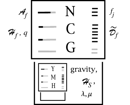
Figure 6: Connes’ slot machine

To see how the Higgs representation derives in general from the fluctuating Dirac operator ${\cal D}$, we must write it as ‘flat’ Dirac operator $\tilde{\cal D}$ plus internal 1-form $H$ like we have done in equation (150) for the minimax example without extension. Take the extended lift ${\mathbb{L}}(w)=\rho(w)J\rho(w)J^{-1}$ with the unitary

$$w = \prod_{j_{1}=1}^{N}(\det w_{j_{1}})^{\tilde{q}_{1j_{1}}},...,\prod_{j_{M}=1}^{N}(\det w_{j_{M}})^{\tilde{q}_{Mj_{M}}},$$ (217)

$$w_{1}\prod_{j_{M+1}=1}^{N}(\det w_{j_{M+1}})^{\tilde{q}_{{M+1},j_{M+1}}},...,w_{N}\prod_{j_{N+M}=1}^{N}(\det w_{j_{N+M}})^{\tilde{q}_{{N+M},j_{N+M}}}.$$

Then

$${\cal D} ={\mathbb{L}}\tilde{\cal D}{\mathbb{L}}^{-1}$$ (223)

$$=\left(\rho(w)\,J\rho(w)J^{-1}\right)\,\tilde{\cal D}\,\left(\rho(w)\,J\rho(w)J^{-1}\right)^{-1}=\rho(w)\,J\rho(w)J^{-1}\tilde{\cal D}\,\rho(w^{-1})\,J\rho(w^{-1})J^{-1}$$

$$=\rho(w)J\rho(w)J^{-1}(\rho(w^{-1})\tilde{\cal D}+[\tilde{\cal D},\rho(w^{-1})])J\rho(w^{-1})J^{-1}$$

$$=J\rho(w)J^{-1}\tilde{\cal D}J\rho(w^{-1})J^{-1}+\rho(w)[\tilde{\cal D},\rho(w^{-1})]=J\rho(w)\tilde{\cal D}\rho(w^{-1})J^{-1}+\rho(w)[\tilde{\cal D},\rho(w^{-1})]$$

$$=J(\rho(w)[\tilde{\cal D},\rho(w^{-1})]+\tilde{\cal D})J^{-1}+\rho(w)[\tilde{\cal D},\rho(w^{-1})]$$

$$=\tilde{\cal D}\,+\,H\,+\,JHJ^{-1},$$

with the internal 1-form, the Higgs scalar, $H=\rho(w)[\tilde{\cal D},\rho(w^{-1})]$. In the chain (223) we have used successively the following three axioms of spectral triples, $[\rho(a),J\rho(\tilde{a})J^{-1}]=0$, the first order condition $[[\tilde{\cal D},\rho(a)],J\rho(\tilde{a})J^{-1}]=0$ and $[\tilde{\cal D},J]=0$. Note that the unitaries, whose representation commutes with the internal Dirac operator, drop out from the Higgs, it transforms as a singlet under their subgroup.

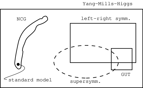
Figure 7: Pseudo forces from noncommutative geometry

The constraints from the axioms of noncommutative geometry are so tight that only very few Yang-Mills-Higgs models can be derived from noncommutative geometry as pseudo forces. No left-right symmetric model can [41], no Grand Unified Theory can [42], for instance the $SU(5)$ model needs 10-dimensional fermion representations, $SO(10)$ 16-dimensional ones, $E_{6}$ is not the group of an associative algebra. Moreover the last two models are left-right symmetric. Much effort has gone into the construction of a supersymmetric model from noncommutative geometry, in vain [43]. The standard model on the other hand fits perfectly into Connes’ picture, Figure 7.

6.3 The standard model

The first noncommutative formulation of the standard model was published by Connes & Lott [33] in 1990. Since then it has evolved into its present form [18, 19, 20, 28] and triggered quite an amount of literature [44].

6.3.1 Spectral triple

The internal algebra ${\cal A}$ is chosen as to reproduce $SU(2)\times U(1)\times SU(3)$ as subgroup of $U({\cal A})$,

$${\cal A}={{\mathbb{H}}}\oplus{\mathbb{C}}\oplus M_{3}({\mathbb{C}})\,\owns\,(a,b,c).$$ (224)

The internal Hilbert space is copied from the Particle Physics Booklet [13],

$${\cal H}_{L} = \left({\mathbb{C}}^{2}\otimes{\mathbb{C}}^{N}\otimes{\mathbb{C}}^{3}\right)\ \oplus\ \left({\mathbb{C}}^{2}\otimes{\mathbb{C}}^{N}\otimes{\mathbb{C}}\right),$$ (225)

$${\cal H}_{R} = \left({\mathbb{C}}\otimes{\mathbb{C}}^{N}\otimes{\mathbb{C}}^{3}\right)\ \oplus\ \left({\mathbb{C}}\otimes{\mathbb{C}}^{N}\otimes{\mathbb{C}}^{3}\right)\ \oplus\ \left({\mathbb{C}}\otimes{\mathbb{C}}^{N}\otimes{\mathbb{C}}\right).$$ (226)

In each summand, the first factor denotes weak isospin doublets or singlets, the second denotes $N$ generations, $N=3$, and the third denotes colour triplets or singlets. Let us choose the following basis of the internal Hilbert space, counting fermions and antifermions (indicated by the superscript $\cdot^{c}$ for ‘charge conjugated’) independently, ${\cal H}={\cal H}_{L}\oplus{\cal H}_{R}\oplus{\cal H}^{c}_{L}\oplus{\cal H}^{c}_{R}={\mathbb{C}}^{90}$:

$$\pmatrix{u\cr d}_{L},\ \pmatrix{c\cr s}_{L},\ \pmatrix{t\cr b}_{L},\ \pmatrix{\nu_{e}\cr e}_{L},\ \pmatrix{\nu_{\mu}\cr\mu}_{L},\ \pmatrix{\nu_{\tau}\cr\tau}_{L};$$ (227)

(228)

$$\matrix{u_{R},\cr d_{R},}\quad\matrix{c_{R},\cr s_{R},}\quad\matrix{t_{R},\cr b_{R},}\quad e_{R},\quad\mu_{R},\quad\tau_{R};$$ (229)

(230)

$$\pmatrix{u\cr d}^{c}_{L},\ \pmatrix{c\cr s}_{L}^{c},\ \pmatrix{t\cr b}_{L}^{c},\ \pmatrix{\nu_{e}\cr e}_{L}^{c},\ \pmatrix{\nu_{\mu}\cr\mu}_{L}^{c},\ \pmatrix{\nu_{\tau}\cr\tau}_{L}^{c};$$ (231)

(232)

$$\matrix{u_{R}^{c},\cr d_{R}^{c},}\quad\matrix{c_{R}^{c},\cr s_{R}^{c},}\quad\matrix{t_{R}^{c},\cr b_{R}^{c},}\quad e_{R}^{c},\quad\mu_{R}^{c},\quad\tau_{R}^{c}.$$

This is the current eigenstate basis, the representation $\rho$ acting on ${\cal H}$ by

$$\rho(a,b,c):=\pmatrix{\rho_{L}&0&0&0\cr 0&\rho_{R}&0&0\cr 0&0&{\bar{\rho}^{c}_{L}}&0\cr 0&0&0&{\bar{\rho}^{c}_{R}}}$$ (233)

with

$$\rho_{L}(a):=\pmatrix{a\otimes 1_{N}\otimes 1_{3}&0\cr 0&a\otimes 1_{N}},\quad\rho_{R}(b):=\pmatrix{b1_{N}\otimes 1_{3}&0&0\cr 0&\bar{b}1_{N}\otimes 1_{3}&0\cr 0&0&\bar{b}1_{N}},$$ (234)

$$\rho^{c}_{L}(b,c):=\pmatrix{1_{2}\otimes 1_{N}\otimes c&0\cr 0&\bar{b}1_{2}\otimes 1_{N}},\quad\rho^{c}_{R}(b,c):=\pmatrix{1_{N}\otimes c&0&0\cr 0&1_{N}\otimes c&0\cr 0&0&\bar{b}1_{N}}.$$ (235)

The apparent asymmetry between particles and antiparticles – the former are subject to weak, the latter to strong interactions – will disappear after application of the lift ${\mathbb{L}}$ with

$$J=\pmatrix{0&1_{15N}\cr 1_{15N}&0}\circ\ {\rm complex\ conjugation}.$$ (236)

For the sake of completeness, we record the chirality as matrix

$$\chi=\pmatrix{-1_{8N}&0&0&0\cr 0&1_{7N}&0&0\cr 0&0&-1_{8N}&0\cr 0&0&0&1_{7N}}.$$ (237)

The internal Dirac operator

$$\tilde{\cal D}=\pmatrix{0&{{\cal M}}&0&0\cr{{\cal M}}^{*}&0&0&0\cr 0&0&0&\bar{{\cal M}}\cr 0&0&\bar{{\cal M}}^{*}&0}$$ (238)

is made of the fermionic mass matrix of the standard model,

$${{\cal M}}=\pmatrix{\pmatrix{1&0\cr 0&0}\otimes M_{u}\otimes 1_{3}\,+\,\pmatrix{0&0\cr 0&1}\otimes M_{d}\otimes 1_{3}&0\cr 0&\pmatrix{0\cr 1}\otimes M_{e}},$$ (239)

with

$$M_{u}:=\pmatrix{m_{u}&0&0\cr 0&m_{c}&0\cr 0&0&m_{t}}, M_{d}:=C_{KM}\pmatrix{m_{d}&0&0\cr 0&m_{s}&0\cr 0&0&m_{b}},$$ (241)

$$M_{e}:=\pmatrix{m_{e}&0&0\cr 0&m_{\mu}&0\cr 0&0&m_{\tau}}.$$

From the booklet we know that all indicated fermion masses are different from each other and that the Cabibbo-Kobayashi-Maskawa matrix $C_{KM}$ is non-degenerate in the sense that no quark is simultaneously mass and weak current eigenstate.

We must acknowledge the fact – and this is far from trivial – that the finite spectral triple of the standard model satisfies all of Connes’ axioms:
$\bullet$ It is orientable, $\chi=\rho(-1_{2},1,1_{3})J\rho(-1_{2},1,1_{3})J^{-1}.$
$\bullet$ Poincaré duality holds. The standard model has three minimal projectors,

$$p_{1}=(1_{2},0,0),\quad p_{2}=(0,1,0),\quad p_{3}=\left(0,0,\pmatrix{1&0&0\cr 0&0&0\cr 0&0&0}\right)$$ (242)

and the intersection form

$$\cap=-2N\pmatrix{0&1&1\cr 1&-1&-1\cr 1&-1&0},$$ (243)

is non-degenerate. We note that Majorana masses are forbidden because of the axiom $\tilde{\cal D}\chi=-\chi\tilde{\cal D}.$ On the other hand if we wanted to give Dirac masses to all three neutrinos we would have to add three right-handed neutrinos to the standard model. Then the intersection form,

$$\cap=-2N\pmatrix{0&1&1\cr 1&-2&-1\cr 1&-1&0},$$ (244)

would become degenerate and Poincaré duality would fail.
$\bullet$ The first order axiom is satisfied precisely because of the first two of the six ad hoc properties of the standard model recalled in subsection 3.3, colour couples vectorially and commutes with the fermionic mass matrix, $[{\cal D},\rho(1_{2},1,c)]=0$. As an immediate consequence the Higgs scalar = internal 1-form will be a colour singlet and the gluons will remain massless, the third ad hoc property of the standard model in its conventional formulation.
$\bullet$ There seems to be some arbitrariness in the choice of the representation under ${\mathbb{C}}\owns b$. In fact this is not true, any choice different from the one in equations (234,235) is either incompatible with the axioms of spectral triples or it leads to charged massless particles incompatible with the Lorentz force or to a symmetry breaking with equal top and bottom masses. Therefore, the only flexibility in the fermionic charges is from the choice of the central charges [40].

6.3.2 Central charges

The standard model has the following groups,

$$U({\cal A})\ = \ SU(2)\times U(1)\times U(3)\quad \owns u=(u_{0},v,w),$$ (245)

$$U^{c}({\cal A})\ = \ {\mathbb{Z}}_{2}\times U(1)\times U(1)\quad \owns u_{c}=(u_{c0},v_{c},w_{c}1_{3}),$$ (246)

$$U^{n}({\cal A})\ = SU(2)\quad\times\quad U(3)\quad \owns\quad\quad\ (u_{0},w),$$ (247)

$$U^{nc}({\cal A})\ = {\mathbb{Z}}_{2}\quad\times\quad U(1)\quad \owns\quad\quad\ (u_{c0},w_{c}1_{3}),$$ (248)

$${\rm Int}({\cal A})\ = \ [SU(2)\quad\times\quad SU(3)]/\Gamma \owns u_{\sigma}=(u_{\sigma 0},w_{\sigma}),$$ (249)

$$\Gamma\ = {\mathbb{Z}}_{2}\quad\times\quad{\mathbb{Z}}_{3}\quad \owns\gamma=(\exp[-m_{0}2\pi i/2],\exp[-m_{2}2\pi i/3]),$$ (250)

with $m_{0}=0,1$ and $m_{2}=0,1,2$. Let us compute the receptacle of the lifted automorphisms,

$${\rm Aut}_{{\cal H}}({\cal A})=[U(2)_{L}\times U(3)_{c} \!\!\!\!\!\!\!\times U(N)_{qL}\times U(N)_{\ell L}\times U(N)_{uR}\times U(N)_{dR}]/[U(1)\times U(1)]$$ (252)

$$\times U(N)_{eR}.$$

The subscripts indicate on which multiplet the $U(N)$s act. The kernel of the projection down to the automorphism group Aut(${\cal A})$ is

$${\rm ker}\,p=[U(1)\times U(1) \!\!\!\!\!\!\!\times U(N)_{qL}\times U(N)_{\ell L}\times U(N)_{uR}\times U(N)_{dR}]/[U(1)\times U(1)]$$ (254)

$$\times U(N)_{eR},$$

and its restrictions to the images of the lifts are

$${\rm ker}\,p\cap L({\rm Int}({\cal A}))={\mathbb{Z}}_{2}\times{\mathbb{Z}}_{3},\quad{\rm ker}\,p\cap{\mathbb{L}}(U^{n}({\cal A}))={\mathbb{Z}}_{2}\times U(1).$$ (255)

The kernel of $i$ is ${\mathbb{Z}}_{2}\times U(1)$ in sharp contrast to the kernel of $\hat{L}$, which is trivial. The isospin $SU(2)_{L}$ and the colour $SU(3)_{c}$ are the image of the lift $\hat{L}$. If $q\not=0,$ the image of $\ell$ consists of one $U(1)\owns w_{c}=\exp[i\theta]$ contained in the five flavour $U(N)$s. Its embedding depends on $q$:

$${\mathbb{L}}(1_{2},1,w_{c}1_{3})=\ell(w_{c})=$$ (256)

$${\rm diag}\,( \!\!\!\!u_{qL}1_{2}\otimes 1_{N}\otimes 1_{3},u_{\ell L}1_{2}\otimes 1_{N},u_{uR}1_{N}\otimes 1_{3},u_{dR}1_{N}\otimes 1_{3},u_{eR}1_{N};$$

$$\!\!\!\!\bar{u}_{qL}1_{2}\otimes 1_{N}\otimes 1_{3},\bar{u}_{\ell L}1_{2}\otimes 1_{N},\bar{u}_{uR}1_{N}\otimes 1_{3},\bar{u}_{dR}1_{N}\otimes 1_{3},\bar{u}_{eR}1_{N})$$

with $u_{j}=\exp[iy_{j}\theta]$ and

$$y_{qL}=q_{2},\qquad y_{\ell L}=-q_{1},\qquad y_{uR}=q_{1}+q_{2},\qquad y_{dR}=-q_{1}+q_{2},\qquad y_{eR}=-2q_{1}.$$ (258)

Independently of the embedding, we have indeed derived the three fermionic conditions of the hypercharge fine tuning (61). In other words, in noncommutative geometry the massless electroweak gauge boson necessarily couples vectorially.

Our goal is now to find the minimal extension $\ell$ that renders the extended lift symmetric, ${\mathbb{L}}(-u_{0},-w)={\mathbb{L}}(u_{0},w)$, and that renders ${\mathbb{L}}(1_{2},w)$ single-valued. The first requirement means { $\tilde{q}_{1}=1$ and $\tilde{q}_{2}=0$ } modulo 2, with

$$\pmatrix{\tilde{q}_{1}\cr\tilde{q}_{2}}=\,{\textstyle\frac{1}{3}}\left(\pmatrix{q_{1}\cr q_{2}}-\pmatrix{0\cr 1}\right).$$ (259)

The second requirement means that $\tilde{q}$ has integer coefficients.

The first extension which comes to mind has $q=0$, $\tilde{q}=\pmatrix{0\cr-1/3}$. With respect to the interpretation (207) of the inner automorphisms, one might object that this is not an extension at all. With respect to the generic characterization (194), it certainly is a non-trivial extension. Anyhow it fails both tests. The most general extension that passes both tests has the form

$$\tilde{q}=\pmatrix{2z_{1}+1\cr 2z_{2}},\quad q=\pmatrix{6z_{1}+3\cr 6z_{2}+1},\quad z_{1},z_{2}\in{\mathbb{Z}}.$$ (260)

Consequently, $y_{\ell_{L}}=-q_{1}$ cannot vanish, the neutrino comes out electrically neutral in compliance with the Lorentz force. As common practise, we normalize the hypercharges to $y_{\ell_{L}}=-1/2$ and compute the last remaining hypercharge $y_{q_{L}}$,

$$y_{q_{L}}=\,\frac{q_{2}}{2q_{1}}\,={\frac{{\textstyle\frac{1}{6}}+z_{2}}{1+2z_{1}}}.$$ (261)

We can change the sign of $y_{q_{L}}$ by permuting $u$ with $d^{c}$ and $d$ with $u^{c}$. Therefore it is sufficient to take $z_{1}=0,1,2,...$ The minimal such extension, $z_{1}=z_{2}=0$, recovers nature’s choice $y_{q_{L}}={\textstyle\frac{1}{6}}$. Its lift,

$${\mathbb{L}}(u_{0},w)=\rho(u_{0},\det w,w)J\rho(u_{0},\det w,w)J^{-1},$$ (262)

is the anomaly free fermionic representation of the standard model considered as $SU(2)\times U(3)$ Yang-Mills-Higgs model. The double-valuedness of ${\mathbb{L}}$ comes from the discrete group ${\mathbb{Z}}_{2}$ of central quaternionic unitaries $(\pm 1_{2},1_{3})\ \in\ {\mathbb{Z}}_{2}\ \subset\ \Gamma\ \subset\ U^{nc}({\cal A})$. On the other hand, O’Raifeartaigh’s [5] ${\mathbb{Z}}_{2}$ in the group of the standard model (46), $\pm(1_{2},1_{3})\ \in\ {\mathbb{Z}}_{2}\ \subset\ U^{nc}({\cal A})$, is not a subgroup of $\Gamma$. It reflects the symmetry of ${\mathbb{L}}$.

6.3.3 Fluctuating metric

The stage is set now for fluctuating the metric by means of the extended lift. This algorithm answers en passant a long standing question in Yang-Mills theories: To gauge or not to gauge? Given a fermionic Lagrangian, e.g. the one of the standard model, our first reflex is to compute its symmetry group. In noncommutative geometry, this group is simply the internal receptacle (252). The painful question in Yang-Mills theory is what subgroup of this symmetry group should be gauged? For us, this question is answered by the choices of the spectral triple and of the spin lift. Indeed the image of the extended lift is the gauge group. The fluctuating metric promotes its generators to gauge bosons, the $W^{\pm}$, the $Z$, the photon and the gluons. At the same time, the Higgs representation is derived, equation (223):

$$H=\rho(u_{0},\det w,w)[\tilde{\cal D},\rho(u_{0},\det w,w)^{-1}]=\pmatrix{0&\hat{H}&0&0\cr\hat{H}^{*}&0&0&0\cr 0&0&0&0\cr 0&0&0&0}$$ (263)

with

$$\hat{H}=\pmatrix{\pmatrix{h_{1}M_{u}&-\bar{h}_{2}M_{d}\cr h_{2}M_{u}&\bar{h}_{1}M_{d}}\otimes 1_{3}&0\cr 0&\pmatrix{-\bar{h}_{2}M_{e}\cr\bar{h}_{1}M_{e}}\cr}$$ (264)

and

$$\pmatrix{h_{1}&-\bar{h}_{2}\cr h_{2}&\bar{h}_{1}}=\pm u_{0}\pmatrix{\det w&0\cr 0&\det\bar{w}}-1_{2}.$$ (265)

The Higgs is characterized by one complex doublet, $(h_{1},h_{2})^{T}$. Again it will be convenient to pass to the homogeneous Higgs variable,

$${\cal D} = {\mathbb{L}}\tilde{\cal D}{\mathbb{L}}^{-1}=\tilde{\cal D}+H+JHJ^{-1}$$ (266)

$$= \Phi+J\Phi J^{-1}=\pmatrix{0&\hat{\Phi}&0&0\cr\hat{\Phi}^{*}&0&0&0\cr 0&0&0&\bar{\hat{\Phi}}\cr 0&0&\bar{\hat{\Phi}}^{*}&0}$$ (268)

with

$$\hat{\Phi}=\pmatrix{\pmatrix{\varphi_{1}M_{u}&-\bar{\varphi}_{2}M_{d}\cr\varphi_{2}M_{u}&\bar{\varphi}_{1}M_{d}}\otimes 1_{3}&0\cr 0&\pmatrix{-\bar{\varphi}_{2}M_{e}\cr\bar{\varphi}_{1}M_{e}}\cr}=\rho_{L}(\phi){{\cal M}}$$ (269)

and

$$\phi=\pmatrix{\varphi_{1}&-\bar{\varphi}_{2}\cr\varphi_{2}&\bar{\varphi}_{1}}=\pm u_{0}\pmatrix{\det w&0\cr 0&\det\bar{w}}.$$ (270)

In order to satisfy the first order condition, the representation of $M_{3}({\mathbb{C}})\owns c$ had to commute with the Dirac operator. Therefore the Higgs is a colour singlet and the gluons will remain massless. The first two of the six intriguing properties of the standard model listed in subsection 3.3 have a geometric raison d’être, the first order condition. In turn, they imply the third property: we have just shown that the Higgs $\varphi=(\varphi_{1},\varphi_{2})^{T}$ is a colour singlet. At the same time the fifth property follows from the fourth: the Higgs of the standard model is an isospin doublet because of the parity violating couplings of the quaternions ${{\mathbb{H}}}$. Furthermore, this Higgs has hypercharge $y_{\varphi}=-{\textstyle\frac{1}{2}}$ and the last fine tuning of the sixth property (61) also derives from Connes’ algorithm: the Higgs has a component with vanishing electric charge, the physical Higgs, and the photon will remain massless.

In conclusion, in Connes version of the standard model there is only one intriguing input property, the fourth: explicit parity violation in the algebra representation ${\cal H}_{L}\oplus{\cal H}_{R}$, the five others are mathematical consequences.

6.3.4 Spectral action

Computing the spectral action $S_{CC}=f({\cal D}_{t}^{2}/\Lambda^{2})$ in the standard model is not more difficult than in the minimax example, only the matrices are a little bigger,

$${\cal D}_{t}={\mathbb{L}}_{t}\tilde{\cal D}_{t}{\mathbb{L}}_{t}^{-1}=\pmatrix{{\,\hbox{$\partial\!\!\!/$}}_{L}&\gamma_{5}\hat{\Phi}&0&0\cr\gamma_{5}\hat{\Phi}^{*}&{\,\hbox{$\partial\!\!\!/$}}_{R}&0&0\cr 0&0&C{\,\hbox{$\partial\!\!\!/$}}_{L}C^{-1}&\gamma_{5}\bar{\hat{\Phi}}\cr 0&0&\gamma_{5}\bar{\hat{\Phi}}^{*}&C{\,\hbox{$\partial\!\!\!/$}}_{R}C^{-1}}.$$ (271)

The trace of the powers of $\hat{\Phi}$ are computed from the identities $\hat{\Phi}=\rho_{L}(\phi){{\cal M}}$ and $\phi^{*}\phi=\phi\phi^{*}=(|\varphi_{1}|^{2}+|\varphi_{2}|^{2})1_{2}=|\varphi|^{2}1_{2}$ by using that $\rho_{L}$ as a representation respects multiplication and involution.

The spectral action produces the complete action of the standard model coupled to gravity with the following relations for coupling constants:

$$g_{3}^{2}=g_{2}^{2}={\textstyle\frac{9}{N}}\lambda.$$ (272)

Our choice of central charges, $\tilde{q}=(1,0)^{T}$, entails a further relation, $g_{1}^{2}={\textstyle\frac{3}{5}}g_{2}^{2}$, i.e. $\sin^{2}\theta_{w}=3/8$. However only products of the Abelian gauge coupling $g_{1}$ and the hypercharges $y_{j}$ appear in the Lagrangian. By rescaling the central charges, we can rescale the hypercharges and consequently the Abelian coupling $g_{1}$. It seems quite moral that noncommutative geometry has nothing to say about Abelian gauge couplings.

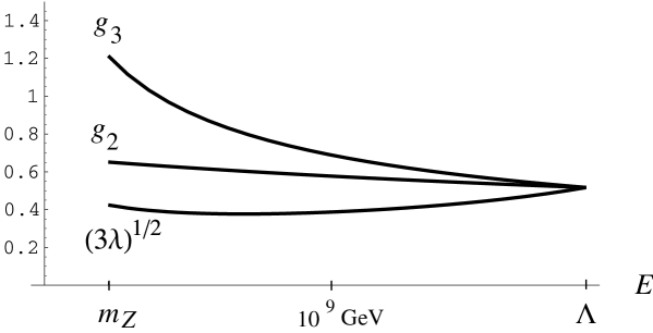
Figure 8: Running coupling constants

Experiment tells us that the weak and strong couplings are unequal, equation (51) at energies corresponding to the $Z$ mass, $g_{2}=0.6518\pm 0.0003,\ g_{3}=1.218\pm 0.01.$ Experiment also tells us that the coupling constants are not constant, but that they evolve with energy. This evolution can be understood theoretically in terms of renormalization: one can get rid of short distance divergencies in perturbative quantum field theory by allowing energy depending gauge, Higgs, and Yukawa couplings where the theoretical evolution depends on the particle content of the model. In the standard model, $g_{2}$ and $g_{3}$ come together with increasing energy, see Figure 8. They would become equal at astronomical energies, $\Lambda=10^{17}$ GeV, if one believed that between presently explored energies, $10^{2}$ GeV, and the ‘unification scale’ $\Lambda$, no new particles exist. This hypothesis has become popular under the name ‘big desert’ since Grand Unified Theories. It was believed that new gauge bosons, ‘lepto-quarks’ with masses of order $\Lambda$ existed. The lepto-quarks together with the $W^{\pm}$, the $Z$, the photon and the gluons generate the simple group $SU(5)$, with only one gauge coupling, $g_{5}^{2}:=g_{3}^{2}=g_{2}^{2}={\textstyle\frac{5}{3}}g_{1}^{2}$ at $\Lambda$. In the minimal $SU(5)$ model, these lepto-quarks would mediate proton decay with a half life that today is excluded experimentally.

If we believe in the big desert, we can imagine that – while almost commutative at present energies – our geometry becomes truly noncommutative at time scales of $\hbar/\Lambda\sim 10^{-41}$ s. Since in such a geometry smaller time intervals cannot be resolved, we expect the coupling constants to become energy independent at the corresponding energy scale $\Lambda$. We remark that the first motivation for noncommutative geometry in spacetime goes back to Heisenberg and was precisely the regularization of short distance divergencies in quantum field theory, see e.g. [45]. The big desert is an opportunistic hypothesis and remains so in the context of noncommutative geometry. But in this context, it has at least the merit of being consistent with three other physical ideas:

Planck time:

There is an old hand waving argument combining Heisenberg’s uncertainty relation of phase space with the Schwarzschild horizon to find an uncertainty relation in spacetime with a scale $\Lambda$ smaller than the Planck energy $(\hbar c^{5}/G)^{1/2}\sim 10^{19}$ GeV: To measure a position with a precision $\Delta x$ we need, following Heisenberg, at least a momentum $\hbar/\Delta x$ or, by special relativity, an energy $\hbar c/\Delta x$. According to general relativity, such an energy creates an horizon of size $G\hbar c^{-3}/\Delta x$. If this horizon exceeds $\Delta x$ all information on the position is lost. We can only resolve positions with $\Delta x$ larger than the Planck length, $\Delta x>(\hbar G/c^{3})^{1/2}\sim 10^{-35}$ m. Or we can only resolve time with $\Delta t$ larger than the Planck time, $\Delta t>(\hbar G/c^{5})^{1/2}\sim 10^{-43}$ s. This is compatible with the above time uncertainty of $\hbar/\Lambda\sim 10^{-41}$ s.

Stability:

We want the Higgs self coupling $\lambda$ to remain positive [46] during its perturbative evolution for all energies up to $\Lambda$. A negative Higgs self coupling would mean that no ground state exists, the Higgs potential is unstable. This requirement is met for the self coupling given by the constraint (272) at energy $\Lambda$, see Figure 8.

Triviality:

We want the Higgs self coupling $\lambda$ to remain perturbatively small [46] during its evolution for all energies up to $\Lambda$ because its evolution is computed from a perturbative expansion. This requirement as well is met for the self coupling given by the constraint (272), see Figure 8. If the top mass was larger than 231 GeV or if there were $N=8$ or more generations this criterion would fail.

Since the big desert gives a minimal and consistent picture we are curious to know its numerical implication. If we accept the constraint (272) with $g_{2}=0.5170$ at the energy $\Lambda=0.968\ 10^{17}$ GeV and evolve it down to lower energies using the perturbative renormalization flow of the standard model, see Figure 8, we retrieve the experimental nonAbelian gauge couplings $g_{2}$ and $g_{3}$ at the $Z$ mass by construction of $\Lambda$. For the Higgs coupling, we obtain

$$\lambda=0.06050\ \pm\ 0.0037\quad{\rm at}\quad E=m_{Z}.$$ (273)

The indicated error comes from the experimental error in the top mass, $m_{t}=174.3\pm 5.1\ {\rm GeV}$, which affects the evolution of the Higgs coupling. From the Higgs coupling at low energies we compute the Higgs mass,

$$m_{H}=4\sqrt{2}\,{\frac{\sqrt{\lambda}}{g_{2}}}\,m_{W}=171.6\ \pm\ 5\ \rm GeV.$$ (274)

For details of this calculation see [47].

6.4 Beyond the standard model

A social reason, that made the Yang-Mills-Higgs machine popular, is that it is an inexhaustible source of employment. Even after the standard model, physicists continue to play on the machine and try out extensions of the standard model by adding new particles, ‘let the desert bloom’. These particles can be gauge bosons coupling only to right-handed fermions in order to restore left-right symmetry. The added particles can be lepto-quarks for grand unification or supersymmetric particles. These models are carefully tuned not to upset the phenomenological success of the standard model. This means in practice to choose Higgs representations and potentials that give masses to the added particles, large enough to make them undetectable in present day experiments, but not too large so that experimentalists can propose bigger machines to test these models. Independently there are always short lived deviations from the standard model predictions in new experiments. They never miss to trigger new, short lived models with new particles to fit the ‘anomalies’. For instance, the literature contains hundreds of superstring inspired Yang-Mills-Higgs models, each of them with hundreds of parameters, coins, waiting for the standard model to fail.

Of course, we are trying the same game in Connes’ do-it-yourself kit. So far, we have not been able to find one single consistent extension of the standard model [41, 42, 43, 48]. The reason is clear, we have no handle on the Higgs representation and potential, which are on the output side, and, in general, we meet two problems: light physical scalars and degenerate fermion masses in irreducible multiplets. The extended standard model with arbitrary numbers of quark generations, $N_{q}\geq 0$, of lepton generations, $N_{\ell}\geq 1$, and of colours $N_{c}$, somehow manages to avoid both problems and we are trying to prove that it is unique as such. The minimax model has $N_{q}=0,\ N_{\ell}=1,\ N_{c}=0$. The standard model has $N_{q}=N_{\ell}=:N$ and $N_{c}=3$ to avoid Yang-Mills anomalies [12]. It also has $N=3$ generations. So far, the only realistic extension of the standard model that we know of in noncommutative geometry, is the addition of right-handed neutrinos and of Dirac masses in one or two generations. These might be necessary to account for observed neutrino oscillations [13].

7 Outlook and conclusion

Noncommutative geometry reconciles Riemannian geometry and uncertainty and we expect it to reconcile general relativity with quantum field theory. We also expect it to improve our still incomplete understanding of quantum field theory. On the perturbative level such an improvement is happening right now: Connes, Moscovici, and Kreimer discovered a subtle link between a noncommutative generalization of the index theorem and perturbative quantum field theory. This link is a Hopf algebra relevant to both theories [49].

In general, Hopf algebras play the same role in noncommutative geometry as Lie groups play in Riemannian geometry and we expect new examples of noncommutative geometry from its merging with the theory of Hopf algebras. Reference [50] contains a simple example where quantum group techniques can be applied to noncommutative particle models.

The running of coupling constants from perturbative quantum field theory must be taken into account in order to perform the high precision test of the standard model at present day energies. We have invoked an extrapolation of this running to astronomical energies to make the constraint $g_{2}=g_{3}$ from the spectral action compatible with experiment. This extrapolation is still based on quantum loops in flat Minkowski space. While acceptable at energies below the scale $\Lambda$ where gravity and the noncommutativity of space seem negligible, this approximation is unsatisfactory from a conceptual point of view and one would like to see quantum fields constructed on a noncommutative space. At the end of the nineties first examples of quantum fields on the (flat) noncommutative torus or its non-compact version, the Moyal plane, were published [51]. These examples came straight from the spectral action. The noncommutative torus is motivated from quantum mechanical phase space and was the first example of a noncommutative spectral triple [52]. Bellissard [53] has shown that the noncommutative torus is relevant in solid state physics: one can understand the quantum Hall effect by taking the Brillouin zone to be noncommutative. Only recently other examples of noncommutative spaces like noncommutative spheres where uncovered [54]. Since 1999, quantum fields on the noncommutative torus are being studied extensively including the fields of the standard model [55]. So far, its internal part is not treated as a noncommutative geometry and Higgs bosons and potentials are added opportunistically. This problem is avoided naturally by considering the tensor product of the noncommutative torus with a finite spectral triple, but I am sure that the axioms of noncommutative geometry can be rediscovered by playing long enough with model building.

In quantum mechanics and in general relativity, time and space play radically different roles. Spatial position is an observable in quantum mechanics, time is not. In general relativity, spacial position loses all meaning and only proper time can be measured. Distances are then measured by a particular observer as (his proper) time of flight of photons going back and forth multiplied by the speed of light, which is supposed to be universal. This definition of distances is operational thanks to the high precision of present day atomic clocks, for example in the GPS. The ‘Riemannian’ definition of the meter, the forty millionth part of a complete geodesic on earth, had to be abandoned in favour of a quantum mechanical definition of the second via the spectrum of an atom. Connes’ definition of geometry via the spectrum of the Dirac operator is the precise counter part of today’s experimental situation. Note that the meter stick is an extended (rigid ?) object. On the other hand an atomic clock is a pointlike object and experiment tells us that the atom is sensitive to the potentials at the location of the clock, the potentials of all forces, gravitational, electro-magnetic, … The special role of time remains to be understood in noncommutative geometry [56] as well as the notion of spectral triples with Lorentzian signature and their 1+3 split [57].

Let us come back to our initial claim: Connes derives the standard model of electro-magnetic, weak and strong forces from noncommutative geometry and, at the same time, unifies them with gravity. If we say that the Balmer-Rydberg formula is derived from quantum mechanics, then this claim has three levels:
Explain the nature of the variables: The choice of the discrete variables $n_{j}$, contains already a – at the time revolutionary – piece of physics, energy quantization. Where does it come from?
Explain the ansatz: Why should one take the power law (11)?
Explain the experimental fit: The ansatz comes with discrete parameters, the ‘bills’ $q_{j}$, and continuous parameters, the ‘coins’ $g_{j}$, which are determined by an experimental fit. Where do the fitted values, ‘the winner’, come from?

How about deriving gravity from Riemannian geometry? Riemannian geometry has only one possible variable, the metric $g$. The minimax principle dictates the Lagrangian ansatz:

$$S[g]=\int_{M}[\Lambda^{c}-{\textstyle\frac{1}{16\pi G}}R^{q}]\,\hbox{\rm d}V.$$ (275)

Experiment rules on the parameters: $q=1$, $G=6.670\cdot 10^{-11}\ \rm m^{3}s^{-2}kg$, Newton’s constant, and $\Lambda^{c}\sim 0$. Riemannian geometry remains silent on the third level. Nevertheless, there is general agreement, gravity derives from Riemannian geometry.

Noncommutative geometry has only one possible variable, the Dirac operator, which in the commutative case coincides with the metric. Its fluctuations explain the variables of the additional forces, gauge and Higgs bosons. The minimax principle dictates the Lagrangian ansatz: the spectral action. It reproduces the Einstein-Hilbert action and the ansatz of Yang, Mills and Higgs, see Table 3. On the third level, noncommutative geometry is not silent, it produces lots of constraints, all compatible with the experimental fit. And their exploration is not finished yet.

Table 3: Deriving some YMH forces from gravity

I hope to have convinced one or the other reader that noncommutative geometry contains elegant solutions of long standing problems in fundamental physics and that it proposes concrete strategies to tackle the remaining ones. I would like to conclude our outlook with a sentence by Planck who tells us how important the opinion of our young, unbiased colleagues is. Planck said, a new theory is accepted, not because the others are convinced, because they die.

It is a pleasure to thank Eike Bick and Frank Steffen for the organization of a splendid School. I thank the participants for their unbiased criticism and Kurusch Ebrahimi-Fard, Volker Schatz, and Frank Steffen for a careful reading of the manuscript.

8 Appendix

8.1 Groups

Groups are an extremely powerful tool in physics. Most symmetry transformations form a group. Invariance under continuous transformation groups entails conserved quantities, like energy, angular momentum or electric charge.

A group G is a set equipped with an associative, not necessarily commutative (or ‘Abelian’) multiplication law that has a neutral element 1. Every group element $g$ is supposed to have an inverse $g^{-1}.$

We denote by ${\mathbb{Z}}_{n}$ the cyclic group of $n$ elements. You can either think of ${\mathbb{Z}}_{n}$ as the set $\{0,1,...,n-1\}$ with multiplication law being addition modulo $n$ and neutral element 0. Or equivalently, you can take the set $\{1,\exp(2\pi i/n),\exp(4\pi i/n),...,\exp((n-1)2\pi i/n)\}$ with multiplication and neutral element 1. ${\mathbb{Z}}_{n}$ is an Abelian subgroup of the permutation group on $n$ objects.

Other immediate examples are matrix groups: The general linear groups $GL(n,{\mathbb{C}})$ and $GL(n,{\mathbb{R}})$ are the sets of complex (real), invertible $n\times n$ matrices. The multiplication law is matrix multiplication and the neutral element is the $n\times n$ unit matrix $1_{n}$. There are many important subgroups of the general linear groups: $SL(n,\cdot)$, $\cdot={\mathbb{R}}$ or ${\mathbb{C}}$, consist only of matrices with unit determinant. $S$ stands for special and will always indicate that we add the condition of unit determinant. The orthogonal group $O(n)$ is the group of real $n\times n$ matrices $g$ satisfying $gg^{T}=1_{n}$. The special orthogonal group $SO(n)$ describes the rotations in the Euclidean space ${\mathbb{R}}^{n}$. The Lorentz group $O(1,3)$ is the set of real $4\times 4$ matrices $g$ satisfying $g\eta g^{T}=\eta$, with $\eta=$diag$\{1,-1,-1,-1\}$. The unitary group $U(n)$ is the set of complex $n\times n$ matrices $g$ satisfying $gg^{*}=1_{n}$. The unitary symplectic group $USp(n)$ is the group of complex $2n\times 2n$ matrices $g$ satisfying $gg^{*}=1_{2n}$ and $g{\cal I}g^{T}={\cal I}$ with

$${\cal I}:=\pmatrix{\pmatrix{0&1\cr-1&0}&\cdots&0\cr\vdots&\ddots&\vdots\cr 0&\cdots&\pmatrix{0&1\cr-1&0}}.$$ (276)

The center $Z(G)$ of a group $G$ consists of those elements in $G$ that commute with all elements in $G$, $Z(G)=\{z\in G,zg=gz\ {\rm for\ all}\ g\in G\}$. For example, $Z(U(n))=U(1)\owns\exp(i\theta)\,1_{n},$ $Z(SU(n))={\mathbb{Z}}_{n}\owns\exp(2\pi ik/n)\,1_{n}$.

All matrix groups are subsets of ${\mathbb{R}}^{2n^{2}}$ and therefore we can talk about compactness of these groups. Recall that a subset of ${\mathbb{R}}^{N}$ is compact if and only if it is closed and bounded. For instance, $U(1)$ is a circle in ${\mathbb{R}}^{2}$ and therefore compact. The Lorentz group on the other hand is unbounded because of the boosts.

The matrix groups are Lie groups which means that they contain infinitesimal elements $X$ close to the neutral element: $\exp X=1+X+O(X^{2})\in G.$ For instance,

$$X=\pmatrix{0&\epsilon&0\cr-\epsilon&0&0\cr 0&0&0},\quad\epsilon\ \rm small,$$ (277)

describes an infinitesimal rotation around the $z$-axis by an infinitesimal angle $\epsilon$. Indeed

$$\exp X=\pmatrix{\cos\epsilon&\sin\epsilon&0\cr-\sin\epsilon&\cos\epsilon&0\cr 0&0&1}\ \in SO(3),\quad 0\leq\epsilon<2\pi,$$ (278)

is a rotation around the $z$-axis by an arbitrary angle $\epsilon$. The infinitesimal transformations $X$ of a Lie group $G$ form its Lie algebra ${\mathfrak{g}}$. It is closed under the commutator $[X,Y]=XY-YX$. For the above matrix groups the Lie algebras are denoted by lower case letters. For example, the Lie algebra of the special unitary group $SU(n)$ is written as $su(n)$. It is the set of complex $n\times n$ matrices $X$ satisfying $X+X^{*}=0$ and ${\rm tr}\,X=0$. Indeed, $1_{n}=(1_{n}+X+...)(1_{n}+X+...)^{*}=1_{n}+X+X^{*}+O(X^{2})$ and $1=\det\exp X=\exp{\rm tr}\,X$. Attention, although defined in terms of complex matrices, $su(n)$ is a real vector space. Indeed, if a matrix $X$ is anti-Hermitean, $X+X^{*}=0$, then in general, its complex scalar multiple $iX$ is no longer anti-Hermitean.

However, in real vector spaces, eigenvectors do not always exist and we will have to complexify the real vector space ${\mathfrak{g}}$: Take a basis of ${\mathfrak{g}}$. Then ${\mathfrak{g}}$ consists of linear combinations of these basis vectors with real coefficients. The complexification ${\mathfrak{g}}^{\mathbb{C}}$ of ${\mathfrak{g}}$ consists of linear combinations with complex coefficients.

The translation group of ${\mathbb{R}}^{n}$ is ${\mathbb{R}}^{n}$ itself. The multiplication law now is vector addition and the neutral element is the zero vector. As the vector addition is commutative, the translation group is Abelian.

The diffeomorphism group Diff$(M)$ of an open subset $M$ of ${\mathbb{R}}^{n}$ (or of a manifold) is the set of differentiable maps $\sigma$ from $M$ into itself that are invertible (for the composition $\circ$) and such that its inverse is differentiable. (Attention, the last condition is not automatic, as you see by taking $M={\mathbb{R}}\owns x$ and $\sigma(x)=x^{3}$.) By virtue of the chain rule we can take the composition as multiplication law. The neutral element is the identity map on $M$, $\sigma=1_{M}$ with $1_{M}(x)=x$ for all $x\in M$.

8.2 Group representations

We said that $SO(3)$ is the rotation group. This needs a little explanation. A rotation is given by an axis, that is a unit eigenvector with unit eigenvalue, and an angle. Two rotations can be carried out one after the other, we say ‘composed’. Note that the order is important, we say that the 3-dimensional rotation group is nonAbelian. If we say that the rotations form a group, we mean that the composition of two rotations is a third rotation. However, it is not easy to compute the multiplication law, i.e., compute the axis and angle of the third rotation as a function of the axes and angles of the two initial rotations. The equivalent ‘representation’ of the rotation group as $3\times 3$ matrices is much more convenient because the multiplication law is simply matrix multiplication. There are several ‘representations’ of the $3$-dimensional rotation group in terms of matrices of different sizes, say $N\times N$. It is sometimes useful to know all these representations. The $N\times N$ matrices are linear maps, ‘endomorphisms’, of the $N$-dimensional vector space ${\mathbb{R}}^{N}$ into itself. Let us denote by End$({\mathbb{R}}^{N})$ the set of all these matrices. By definition, a representation of the group $G$ on the vector space ${\mathbb{R}}^{N}$ is a map $\rho:G\rightarrow{\rm End}({\mathbb{R}}^{N})$ reproducing the multiplication law as matrix multiplication or in nobler terms as composition of endomorphisms. This means $\rho(g_{1}g_{2})=\rho(g_{1})\,\rho(g_{2})$ and $\rho(1)=1_{N}$. The representation is called faithful if the map $\rho$ is injective. By the minimax principle we are interested in the faithful representations of lowest dimension. Although not always unique, physicists call them fundamental representations. The fundamental representation of the $3$-dimensional rotation group is defined on the vector space ${\mathbb{R}}^{3}$. Two $N$-dimensional representations $\rho_{1}$ and $\rho_{2}$ of a group $G$ are equivalent if there is an invertible $N\times N$ matrix $C$ such that $\rho_{2}(g)=C\rho_{1}(g)C^{-1}$ for all $g\in G$. $C$ is interpreted as describing a change of basis in ${\mathbb{R}}^{N}$. A representation is called irreducible if its vector space has no proper invariant subspace, i.e. a subspace $W\subset{\mathbb{R}}^{N}$, with $W\not={\mathbb{R}}^{N},\{0\}$ and $\rho(g)W\subset W$ for all $g\in G$.

Representations can be defined in the same manner on complex vector spaces, ${\mathbb{C}}^{N}$. Then every $\rho(g)$ is a complex, invertible matrix. It is often useful, e.g. in quantum mechanics, to represent a group on a Hilbert space, we put a scalar product on the vector space, e.g. the standard scalar product on ${\mathbb{C}}^{N}\owns v,w$, $(v,w):=v^{*}w$. A unitary representation is a representation whose matrices $\rho(g)$ all respect the scalar product, which means that they are all unitary. In quantum mechanics, unitary representations are important because they preserve probability. For example, take the adjoint representation of $SU(n)\owns g$. Its Hilbert space is the complexification of its Lie algebra $su(n)^{\mathbb{C}}\owns X,Y$ with scalar product $(X,Y):={\rm tr}\,(X^{*}Y)$. The representation is defined by conjugation, $\rho(g)X:=gXg^{-1}$, and it is unitary, $(\rho(g)X,\rho(g)Y)=(X,Y)$. In Yang-Mills theories, the gauge bosons live in the adjoint representation. In the Abelian case, $G=U(1)$, this representation is 1-dimensional, there is one gauge boson, the photon, $A\in u(1)^{\mathbb{C}}={\mathbb{C}}.$ The photon has no electric charge, which means that it transforms trivially, $\rho(g)A=A$ for all $g\in U(1)$.

Unitary equivalence of representations is defined by change of orthonormal bases. Then $C$ is a unitary matrix. A key theorem for particle physics states that all irreducible unitary representations of any compact group are finite dimensional. If we accept the definition of elementary particles as orthonormal basis vectors of unitary representations, then we understand why Yang and Mills only take compact groups. They only want a finite number of elementary particles. Unitary equivalence expresses the quantum mechanical superposition principle observed for instance in the $K^{0}-\bar{K}^{0}$ system. The unitary matrix $C$ is sometimes referred to as mixing matrix.

Bound states of elementary particles are described by tensor products: the tensor product of two unitary representations $\rho_{1}$ and $\rho_{2}$ of one group defined on two Hilbert spaces ${\cal H}_{1}$ and ${\cal H}_{2}$ is the unitary representation $\rho_{1}\otimes\rho_{2}$ defined on ${\cal H}_{1}\otimes{\cal H}_{2}\owns\psi_{1}\otimes\psi_{2}$ by $(\rho_{1}\otimes\rho_{2})(g)\,(\psi_{1}\otimes\psi_{2}):=\rho_{1}(g)\,\psi_{1}\otimes\rho_{2}(g)\,\psi_{2}$. In the case of electro-magnetism, $G=U(1)\owns\exp(i\theta)$ we know that all irreducible unitary representations are 1-dimensional, ${\cal H}={\mathbb{C}}\owns\psi$ and characterized by the electric charge $q$, $\rho(\exp(i\theta))\psi=\exp(iq\psi)\psi$. Under tensorization the electric charges are added. For $G=SU(2)$, the irreducible unitary representations are characterized by the spin, $\ell=0,{\textstyle\frac{1}{2}},1,...$ The addition of spin from quantum mechanics is precisely tensorization of these representations.

Let $\rho$ be a representation of a Lie group $G$ on a vector space and let ${\mathfrak{g}}$ be the Lie algebra of $G$. We denote by $\tilde{\rho}$ the Lie algebra representation of the group representation $\rho$. It is defined on the same vector space by $\rho(\exp X)=\exp(\tilde{\rho}(X))$. The $\tilde{\rho}(X)$s are not necessarily invertible endomorphisms. They satisfy $\tilde{\rho}([X,Y])=[\tilde{\rho}(X),\tilde{\rho}(Y)]:=\tilde{\rho}(X)\tilde{\rho}(Y)-\tilde{\rho}(Y)\tilde{\rho}(X).$

An affine representation is the same construction as above, but we allow the $\rho(g)$s to be invertible affine maps, i.e. linear maps plus constants.

8.3 Semi-direct product and Poincaré group

The direct product $G\times H$ of two groups $G$ and $H$ is again a group with multiplication law: $(g_{1},h_{1})(g_{2},h_{2}):=(g_{1}g_{2},h_{1}h_{2}).$ In the direct product, all elements of the first factor commute with all elements of the second factor: $(g,1^{H})(1^{G},h)=(1^{G},h)(g,1^{H}).$ We write $1^{H}$ for the neutral element of $H$. Warning, you sometimes see the misleading notation $G\otimes H$ for the direct product.

To be able to define the semi-direct product $G\ltimes H$ we must have an action of $G$ on $H$, that is a map $\rho:G\rightarrow{\rm Diff}(H)$ satisfying $\rho_{g}(h_{1}h_{2})=\rho_{g}(h_{1})\,\rho_{g}(h_{2})$, $\rho_{g}(1^{H})=1^{H}$, $\rho_{g_{1}g_{2}}=\rho_{g_{1}}\circ\rho_{g_{2}}$ and $\rho_{1^{G}}=1_{H}$. If $H$ is a vector space carrying a representation or an affine representation $\rho$ of the group $G$, we can view $\rho$ as an action by considering $H$ as translation group. Indeed, invertible linear maps and affine maps are diffeomorphisms on $H$. As a set, the semi-direct product $G\ltimes H$ is the direct product, but the multiplication law is modified by help of the action:

$$(g_{1},h_{1})(g_{2},h_{2}):=(g_{1}g_{2},h_{1}\,\rho_{g_{1}}(h_{2})).$$ (279)

We retrieve the direct product if the action is trivial, $\rho_{g}=1_{H}$ for all $g\in G$. Our first example is the invariance group of electro-magnetism coupled to gravity ${\rm Diff}(M)\ltimes\,^{M}U(1).$ A diffeomorphism $\sigma(x)$ acts on a gauge function $g(x)$ by $\rho_{\sigma}(g):=g\circ\sigma^{-1}$ or more explicitly $(\rho_{\sigma}(g))(x):=g(\sigma^{-1}(x))$. Other examples come with other gauge groups like $SU(n)$ or spin groups.

Our second example is the Poincaré group, $O(1,3)\ltimes{\mathbb{R}}^{4}$, which is the isometry group of Minkowski space. The semi-direct product is important because Lorentz transformations do not commute with translations. Since we are talking about the Poincaré group, let us mention the theorem behind the definition of particles as orthonormal basis vectors of unitary representations: The irreducible, unitary representations of the Poincaré group are characterized by mass and spin. For fixed mass $M\geq 0$ and spin $\ell$, an orthonormal basis is labelled by the momentum $\vec{p}$ with $E^{2}/c^{2}-\vec{p}^{2}=c^{2}M^{2}$, $\psi=\exp(i(Et-\vec{p}\cdot\vec{x})/\hbar)$ and the $z$-component $m$ of the spin with $|m|\leq\ell$, $\psi=Y_{\ell,m}(\theta,\varphi)$.

8.4 Algebras

Observables can be added, multiplied and multiplied by scalars. They form naturally an associative algebra ${\cal A}$, i.e. a vector space equipped with an associative product and neutral elements 0 and 1. Note that the multiplication does not always admit inverses, $a^{-1}$, e.g. the neutral element of addition, 0, is not invertible. In quantum mechanics, observables are self adjoint. Therefore, we need an involution $\cdot^{*}$ in our algebra. This is an anti-linear map from the algebra into itself, $(\lambda a+b)^{*}=\bar{\lambda}a^{*}+b^{*},\ \lambda\in{\mathbb{C}},\ a,b\in{\cal A},$ that reverses the product, $(ab)^{*}=b^{*}a^{*}$, respects the unit, $1^{*}=1$, and is such that $a^{**}=a$. The set of $n\times n$ matrices with complex coefficients, $M_{n}({\mathbb{C}})$, is an example of such an algebra, and more generally, the set of endomorphisms or operators on a given Hilbert space ${\cal H}$. The multiplication is matrix multiplication or more generally composition of operators, the involution is Hermitean conjugation or more generally the adjoint of operators.

A representation $\rho$ of an abstract algebra ${\cal A}$ on a Hilbert space ${\cal H}$ is a way to write ${\cal A}$ concretely as operators as in the last example, $\rho:{\cal A}\rightarrow{\rm End}({\cal H})$. In the group case, the representation had to reproduce the multiplication law. Now it has to reproduce, the linear structure: $\rho(\lambda a+b)=\lambda\rho(a)+\rho(b),\ \rho(0)=0,$ the multiplication: $\rho(ab)=\rho(a)\rho(b),\ \rho(1)=1,$ and the involution: $\rho(a^{*})=\rho(a)^{*}.$ Therefore the tensor product of two representations $\rho_{1}$ and $\rho_{2}$ of ${\cal A}$ on Hilbert spaces ${\cal H}_{1}\owns\psi_{1}$ and ${\cal H}_{2}\owns\psi_{2}$ is not a representation: $((\rho_{1}\otimes\rho_{2})(\lambda a))\,(\psi_{1}\otimes\psi_{2})=(\rho_{1}(\lambda a)\,\psi_{1})\otimes(\rho_{2}(\lambda a)\,\psi_{2})=\lambda^{2}(\rho_{1}\otimes\rho_{2})(a)\,(\psi_{1}\otimes\psi_{2})$.

The group of unitaries $U({\cal A}):=\{u\in{\cal A},\,uu^{*}=u^{*}u=1\}$ is a subset of the algebra ${\cal A}$. Every algebra representation induces a unitary representation of its group of unitaries. On the other hand, only few unitary representations of the group of unitaries extend to an algebra representation. These representations describe elementary particles. Composite particles are described by tensor products, which are not algebra representations.

An anti-linear operator $J$ on a Hilbert space ${\cal H}\owns\psi,\tilde{\psi}$ is a map from ${\cal H}$ into itself satisfying $J(\lambda\psi+\tilde{\psi})=\bar{\lambda}J(\psi)+J(\tilde{\psi}).$ An anti-linear operator $J$ is anti-unitary if it is invertible and preserves the scalar product, $(J\psi,J\tilde{\psi})=(\tilde{\psi},\psi)$. For example, on ${\cal H}={\mathbb{C}}^{n}\owns\psi$ we can define an anti-unitary operator $J$ in the following way. The image of the column vector $\psi$ under $J$ is obtained by taking the complex conjugate of $\psi$ and then multiplying it with a unitary $n\times n$ matrix $U$, $J\psi=U\bar{\psi}$ or $J=\,U\,\circ$ complex conjugation. In fact, on a finite dimensional Hilbert space, every anti-unitary operator is of this form.

References

- [1] A. Connes, A. Lichnérowicz & M. P. Schützenberger, Triangle de Pensées, O. Jacob (2000), English version: Triangle of Thoughts, AMS (2001)
- [2] G. Amelino-Camelia, Are we at the dawn of quantum gravity phenomenology? Lectures given at 35th Winter School of Theoretical Physics: From Cosmology to Quantum Gravity, Polanica, Poland, 1999, gr-qc/9910089
-
[3]
S. Weinberg, Gravitation and Cosmology, Wiley (1972)
R. Wald, General Relativity, The University of Chicago Press (1984) - [4] J. D. Bjørken & S. D. Drell, Relativistic Quantum Mechanics, McGraw–Hill (1964)
- [5] L. O’Raifeartaigh, Group Structure of Gauge Theories, Cambridge University Press (1986)
- [6] M. Göckeler & T. Schücker, Differential Geometry, Gauge Theories, and Gravity, Cambridge University Press (1987)
-
[7]
R. Gilmore, Lie Groups, Lie Algebras and Some of Their
Applications, Wiley (1974)
H. Bacry, Lectures Notes in Group Theory and Particle Theory, Gordon and Breach (1977) - [8] N. Jacobson, Basic Algebra I, II, Freeman (1974, 1980)
-
[9]
J. Madore, An Introduction to Noncommutative
Differential Geometry and Its Physical Applications,
Cambridge University Press (1995)
G. Landi, An Introduction to Noncommutative Spaces and Their Geometry, hep-th/9701078, Springer (1997) - [10] J. M. Gracia-Bondía, J. C. Várilly & H. Figueroa, Elements of Noncommutative Geometry, Birkhäuser (2000)
- [11] J. W. van Holten, Aspects of BRST quantization, hep-th/0201124, in this volume
- [12] J. Zinn-Justin, Chiral anomalies and topology, hep-th/0201220, in this volume
- [13] The Particle Data Group, Particle Physics Booklet and http://pdg.lbl.gov
-
[14]
G. ’t Hooft, Renormalizable Lagrangians for massive
Yang-Mills fields, Nucl. Phys. B35 (1971) 167
G. ’t Hooft & M. Veltman, Regularization and renormalization of gauge fields, Nucl. Phys. B44 (1972) 189
G. ’t Hooft & M. Veltman, Combinatorics of gauge fields, Nucl. Phys. B50 (1972) 318
B. W. Lee & J. Zinn-Justin, Spontaneously broken gauge symmetries I, II, III and IV, Phys. Rev. D5 (1972) 3121, 3137, 3155, Phys. Rev. D7 (1973) 1049 -
[15]
S. Glashow, Partial-symmetries of weak interactions, Nucl.
Phys. 22 (1961) 579
A. Salam in Elementary Particle Physics: Relativistic Groups and Analyticity, Nobel Symposium no. 8, page 367, eds.: N. Svartholm, Almqvist & Wiksell, Stockholm 1968
S. Weinberg, A model of leptons, Phys. Rev. Lett. 19 (1967) 1264 - [16] J. Iliopoulos, An introduction to gauge theories, Yellow Report, CERN (1976)
- [17] G. Esposito-Farèse, Théorie de Kaluza-Klein et gravitation quantique, Thése de Doctorat, Université d’Aix-Marseille II, 1989
- [18] A. Connes, Noncommutative Geometry, Academic Press (1994)
- [19] A. Connes, Noncommutative geometry and reality, J. Math. Phys. 36 (1995) 6194
- [20] A. Connes, Gravity coupled with matter and the foundation of noncommutative geometry, hep-th/9603053, Comm. Math. Phys. 182 (1996) 155
- [21] H. Rauch, A. Zeilinger, G. Badurek, A. Wilfing, W. Bauspiess & U. Bonse, Verification of coherent spinor rotations of fermions, Phys. Lett. 54A (1975) 425
- [22] E. Cartan, Leçons sur la théorie des spineurs, Hermann (1938)
-
[23]
A. Connes, Brisure de symétrie spontanée et géométrie du
point de vue spectral, Séminaire Bourbaki, 48ème année, 816 (1996)
313
A. Connes, Noncommutative differential geometry and the structure of space time, Operator Algebras and Quantum Field Theory, eds.: S. Doplicher et al., International Press, 1997 - [24] T. Schücker, Spin group and almost commutative geometry, hep-th/0007047
- [25] J.-P. Bourguignon & P. Gauduchon, Spineurs, opérateurs de Dirac et variations de métriques, Comm. Math. Phys. 144 (1992) 581
- [26] U. Bonse & T. Wroblewski, Measurement of neutron quantum interference in noninertial frames, Phys. Rev. Lett. 1 (1983) 1401
- [27] R. Colella, A. W. Overhauser & S. A. Warner, Observation of gravitationally induced quantum interference, Phys. Rev. Lett. 34 (1975) 1472
- [28] A. Chamseddine & A. Connes, The spectral action principle, hep-th/9606001, Comm. Math. Phys.186 (1997) 731
- [29] G. Landi & C. Rovelli, Gravity from Dirac eigenvalues, gr-qc/9708041, Mod. Phys. Lett. A13 (1998) 479
-
[30]
P. B. Gilkey, Invariance Theory, the Heat Equation,
and the Atiyah-Singer Index Theorem, Publish or
Perish (1984)
S. A. Fulling, Aspects of Quantum Field Theory in Curved Space-Time, Cambridge University Press (1989) - [31] B. Iochum, T. Krajewski & P. Martinetti, Distances in finite spaces from noncommutative geometry, hep-th/9912217, J. Geom. Phys. 37 (2001) 100
- [32] M. Dubois-Violette, R. Kerner & J. Madore, Gauge bosons in a noncommutative geometry, Phys. Lett. 217B (1989) 485
-
[33]
A. Connes, Essay on physics and noncommutative
geometry, in The Interface of Mathematics and
Particle Physics, eds.: D. G. Quillen et al., Clarendon
Press (1990)
A. Connes & J. Lott, Particle models and noncommutative geometry, Nucl. Phys. B 18B (1990) 29
A. Connes & J. Lott, The metric aspect of noncommutative geometry, in the proceedings of the 1991 Cargèse Summer Conference, eds.: J. Fröhlich et al., Plenum Press (1992) - [34] J. Madore, Modification of Kaluza Klein theory, Phys. Rev. D 41 (1990) 3709
- [35] P. Martinetti & R. Wulkenhaar, Discrete Kaluza-Klein from scalar fluctuations in noncommutative geometry, hep-th/0104108, J. Math. Phys. 43 (2002) 182
-
[36]
T. Ackermann & J. Tolksdorf, A generalized
Lichnerowicz formula, the Wodzicki residue and
gravity, hep-th/9503152, J. Geom. Phys. 19 (1996) 143
T. Ackermann & J. Tolksdorf, The generalized Lichnerowicz formula and analysis of Dirac operators, hep-th/9503153, J. reine angew. Math. 471 (1996) 23 - [37] R. Estrada, J. M. Gracia-Bondía & J. C. Várilly, On summability of distributions and spectral geometry, funct-an/9702001, Comm. Math. Phys. 191 (1998) 219
-
[38]
B. Iochum, D. Kastler & T. Schücker, On the universal Chamseddine-Connes action:
details of the action computation, hep-th/9607158,
J. Math. Phys. 38 (1997) 4929
L. Carminati, B. Iochum, D. Kastler & T. Schücker, On Connes’ new principle of general relativity: can spinors hear the forces of space-time?, hep-th/9612228, Operator Algebras and Quantum Field Theory, eds.: S. Doplicher et al., International Press, 1997 -
[39]
M. Paschke & A. Sitarz, Discrete spectral triples
and their symmetries, q-alg/9612029,
J. Math. Phys. 39 (1998) 6191
T. Krajewski, Classification of finite spectral triples, hep-th/9701081, J. Geom. Phys. 28 (1998) 1 - [40] S. Lazzarini & T. Schücker, A farewell to unimodularity, hep-th/0104038, Phys.Lett. B 510 (2001) 277
-
[41]
B. Iochum & T. Schücker, A left-right symmetric
model à la Connes-Lott, hep-th/9401048, Lett. Math.
Phys. 32 (1994) 153
F. Girelli, Left-right symmetric models in noncommutative geometry? hep-th/0011123, Lett. Math. Phys. 57 (2001) 7 - [42] F. Lizzi, G. Mangano, G. Miele & G. Sparano, Constraints on unified gauge theories from noncommutative geometry, hep-th/9603095, Mod. Phys. Lett. A11 (1996) 2561
- [43] W. Kalau & M. Walze, Supersymmetry and noncommutative geometry, hep-th/9604146, J. Geom. Phys. 22 (1997) 77
-
[44]
D. Kastler, Introduction to noncommutative geometry
and Yang-Mills model building, Differential geometric
methods in
theoretical physics, Rapallo (1990), 25
— , A detailed account of Alain Connes’ version of the standard model in non-commutative geometry, I, II and III, Rev. Math. Phys. 5 (1993) 477, Rev. Math. Phys. 8 (1996) 103 D. Kastler & T. Schücker, Remarks on Alain Connes’ approach to the standard model in non-commutative geometry, Theor. Math. Phys. 92 (1992) 522, English version, 92 (1993) 1075, hep-th/0111234
— , A detailed account of Alain Connes’ version of the standard model in non-commutative geometry, IV, Rev. Math. Phys. 8 (1996) 205
— , The standard model à la Connes-Lott, hep-th/9412185, J. Geom. Phys. 388 (1996) 1
J. C. Várilly & J. M. Gracia-Bondía, Connes’ noncommutative differential geometry and the standard model, J. Geom. Phys. 12 (1993) 223 T. Schücker & J.-M. Zylinski, Connes’ model building kit, hep-th/9312186, J. Geom. Phys. 16 (1994) 1
E. Alvarez, J. M. Gracia-Bondía & C. P. Martín, Anomaly cancellation and the gauge group of the Standard Model in Non-Commutative Geometry, hep-th/9506115, Phys. Lett. B364 (1995) 33
R. Asquith, Non-commutative geometry and the strong force, hep-th/9509163, Phys. Lett. B 366 (1996) 220
C. P. Martín, J. M. Gracia-Bondía & J. C. Várilly, The standard model as a noncommutative geometry: the low mass regime, hep-th/9605001, Phys. Rep. 294 (1998) 363
L. Carminati, B. Iochum & T. Schücker, The noncommutative constraints on the standard model à la Connes, hep-th/9604169, J. Math. Phys. 38 (1997) 1269
R. Brout, Notes on Connes’ construction of the standard model, hep-th/9706200, Nucl. Phys. Proc. Suppl. 65 (1998) 3
J. C. Várilly, Introduction to noncommutative geometry, physics/9709045, EMS Summer School on Noncommutative Geometry and Applications, Portugal, september 1997, ed.: P. Almeida
T. Schücker, Geometries and forces, hep-th/9712095, EMS Summer School on Noncommutative Geometry and Applications, Portugal, september 1997, ed.: P. Almeida
J. M. Gracia-Bondía, B. Iochum & T. Schücker, The Standard Model in Noncommutative Geometry and Fermion Doubling, hep-th/9709145, Phys. Lett. B 414 (1998) 123
D. Kastler, Noncommutative geometry and basic physics, Lect. Notes Phys. 543 (2000) 131