Bits and Pieces in
Logarithmic Conformal Field Theory

Abstract:

These are notes of my lectures held at the first School & Workshop on Logarithmic Conformal Field Theory and its Applications, September 2001 in Tehran, Iran.
These notes cover only selected parts of the by now quite extensive knowledge on logarithmic conformal field theories. In particular, I discuss the proper generalization of null vectors towards the logarithmic case, and how these can be used to compute correlation functions. My other main topic is modular invariance, where I discuss the problem of the generalization of characters in the case of indecomposable representations, a proposal for a Verlinde formula for fusion rules and identities relating the partition functions of logarithmic conformal field theories to such of well known ordinary conformal field theories.
These two main topics are complemented by some remarks on ghost systems, the Haldane-Rezayi fractional quantum Hall state, and the relation of these two to the logarithmic $c=-2$ theory.

1 Introduction

These are notes of my lectures held at the first School & Workshop on Logarithmic Conformal Field Theory and its Applications, which took place at the IPM (Institute for Studies in Theoretical Physics and Mathematics) in Tehran, Iran, 4.-18. September 2001.

During the last few years, so-called logarithmic conformal field theory (LCFT) established itself as a well-defined new animal in the zoo of conformal field theories in two dimensions. These are conformal field theories where, despite scaling invariance, correlation function might exhibit logarithmic divergences. To our knowledge, such logarithmic singularities in correlation functions were first noted by Knizhnik back in 1987 [66], but since LCFT had not been invented (or found) then, he had to discuss them away. The first works we are aware of, which made a clear connection between logarithms in correlation functions, indecomposability of representations and operator product expansions containing logarithmic fields (although they were not called that way then), are three papers by Saleur, and then Rozansky and Saleur, [106, 105]. But it took six years since Knizhnik’s publication, that the concept of a conformal field theory with logarithmic divergent behavior due to logarithmic operators was considered in its own right by Gurarie [48], who got interested in this matter by discussions with A.B. Zamolodchikov. From then one, there has been a considerable amount of work on analyzing the general structure of LCFTs, which by now has generalized almost all of the basic notions and tools of (rational) conformal field theories, such as null vectors, characters, partition functions, fusion rules, modular invariance etc., to the logarithmic case. A complete list of references is already too long even for lectures notes, but see for example [33, 21, 41, 43, 45, 59, 63, 71, 86, 91, 99, 100, 104] and references therein. Besides the best understood main example of the logarithmic theory with central charge $c=-2$, as well as its $c_{p,1}$ relatives, other specific models were considered such as WZW models [3, 42, 70, 95, 96] and LCFTs related to supergroups and supersymmetry [4, 16, 62, 64, 76, 82, 103, 105]. Strikingly, Rozansky and Saleur did note that indecomposable representations should play a rôle in CFT severely influencing the behavior of, for example, the modular $S$- and $T$-matrices, before Gurarie published his work in 1993. The only concept they did not explicitly introduce was that of a Jordan cell structure with respect to $L_{0}$ or other generators in the chiral symmetry algebra.

Also, quite a number of applications have already been pursued, and LCFTs have emerged in many different areas by now. We will hear about some of them in the course of this school. Hence, I mention only some of them, which I found particularly exciting. Sometimes, longstanding puzzles in the description of certain theoretical models could be resolved, e.g. the enigmatic degeneracy of the ground state in the Haldane-Rezayi fractional quantum Hall effect with filling factor $\nu=5/2$, where conformal field theory descriptions of the bulk theory proved difficult [11, 49, 102], multi-fractality in disordered Dirac fermions, where the spectra did not add up correctly as long as logarithmic fields in internal channels were neglected [17], or two-dimensional conformal turbulence, where Polyakov’s proposal of a conformal field theory solution did contradict phenomenological expectations on the energy spectrum [35, 98, 109]. Other applications worth mentioning are gravitational dressing [8], polymers and Abelian sandpiles [13, 56, 84, 106], the (fractional) quantum Hall effect [34, 53, 74], and – perhaps most importantly – disorder [5, 6, 14, 15, 50, 51, 68, 83, 101]. Finally, there are even applications in string theory [67], especially in $D$-brane recoil [10, 24, 26, 47, 69, 77, 79, 87], AdS/CFT correspondence [44, 60, 65, 72, 73, 93, 94, 107], and also in Seiberg-Witten solutions to supersymmetric Yang-Mills theories, e.g. [12, 36, 78], Last, but not least, a recent focus of research on LCFTs is in its boundary conformal field theory aspects [54, 61, 75, 80, 91].

In these note, we will not cover any of the applications, and we will only discuss some of the general issues in LCFT. We will focus mainly on two issues in particular. Firstly, we discuss so-called null states, and how these can help to compute correlation functions in LCFTs. Secondly, we look at modular invariance, whether and how it can be ensured in LCFTs, and what consequences it has on the operator algebra. More precisely, we discuss the problem of the generalization of characters in the case of indecomposable representations, a proposal for a Verlinde formula for fusion rules and identities relating the partition functions of logarithmic conformal field theories to such of well known ordinary conformal field theories.

As already said, these notes cover only selected parts of the by now quite extensive knowledge on logarithmic conformal field theories. On the other hand, we have tried to make these notes rather self-contained, which means that some parts may overlap with other lecture notes for this school, and are included here for convenience. In particular, we did not assume any deeper knowledge of generic common conformal field theory.

• Some parts are set in smaller type, like the paragraph you are just reading. They mostly contain more advanced material and further details which may be skipped upon first reading. Some of these parts, however, contain additional explanations addressed to a reader who is a novice to the vast theme of CFT in general, and may be skipped by readers already familiar with basic conformal field theory techniques.

For those readers completely unfamiliar with CFT in general, we provide a (very) short list of introductory material, for their convenience which, however, is by no means complete. The reviews on string theory which we included in the list contain, in our opinion, quite suitable introductions to certain aspects of conformal field theory.

• L. Alvarez-Gaumé, Helv. Phys. Acta 61 (1991) 359-526.

• J. Cardy, in Les Houches 1988 Summer School, E. Brézin and J. Zinn-Justin, eds. (1989) Elsevier, Amsterdam.

• Ph. Di Francesco, P. Mathieu, D. Sénéchal, Conformal Field Theory, Graduate Texts in Contemporary Physics (1997) Springer.

• R. Dijkgraaf, Les Houches Lectures on Fields, Strings and Duality, to appear [hep-th/9703136].

• J. Fuchs, Lectures on conformal field theory and Kac-Moody algebras, to appear in Lecture Notes in Physics, Springer [hep-th/9702194].

• M. Gaberdiel, Rept. Prog. Phys. 63 (2000) 607-667 [hep-th/9910156].

• P. Ginsparg, in Les Houches 1988 Summer School, E. Brézin and J. Zinn-Justin, eds. (1989) Elsevier, Amsterdam [http://xxx.lanl.gov/hypertex/hyperlh88.tar.gz].

• C. Gomez, M. Ruiz-Altaba, Rivista Del Nuovo Cimento 16 (1993) 1–124.

• M. Green, J. Schwarz, E. Witten, String Theory, vols. 1,2 (1986) Cambridge University Press.

• M. Kaku, String Theory (1988) Springer.

• S.V. Ketov, Conformal Field Theory (1995) World Scientific.

• D. Lüst, S. Theisen, Lectures on String Theory, Lecture Notes in Physics (1989) Springer.

• A.N. Schellekens Conformal Field Theory, Saalburg Summer School lectures (1995) [http://www.itp.uni-hannover.de/~flohr/lectures/schellekens.cft-lectures.ps.gz].

• C. Schweigert, J. Fuchs, J. Walcher, Conformal field theory, boundary conditions and applications to string theory [hep-th/0011109].

• A.B. Zamolodchikov, Al.B. Zamolodchikov, Conformal Field Theory and Critical Phenomena in Two-Dimensional Systems, Soviet Scientific Reviews/Sec. A/Phys. Reviews (1989) Harwood Academic Publishers.

2 CFT proper

In these notes, we will detach ourselves from any string theoretic or condensed matter application motivations and consider CFT solely on its own. This section is a very rudimentary summary of some CFT basics. As mentioned in the basic CFT lectures, it is customary to work on the complex plane (or Riemann sphere) with the holomorphic coordinate $z$ and the holomorphic differential or one-form ${\rm d}z$. A field $\Phi(z)$ is called a conformal or primary field of weight $h$, if it transforms under holomorphic mappings $z\mapsto z^{\prime}(z)$ of the coordinate as

$$\Phi_{h}(z)({\rm d}z)^{h}\mapsto\Phi_{h}(z^{\prime})({\rm d}z^{\prime})^{h}=\Phi_{h}(z)({\rm d}z)^{h}\,.$$ (1)

In case that the conformal weight $h$ is not a (half-)integer, it is better to write this as

$$\Phi_{h}(z)\mapsto\Phi_{h}(z^{\prime})=\Phi_{h}(z)\left(\frac{\partial z^{\prime}(z)}{\partial z}\right)^{-h}\,.$$ (2)

One should keep in mind that all formulæ here have an anti-holomorphic counterpart. Since a primary field factorizes into holomorphic and anti-holomorphic parts, $\Phi_{h,\bar{h}}(z,\bar{z})=\Phi_{h}(z)\Phi_{\bar{h}}(\bar{z})$, in most cases, we can skip half of the story. Infinitesimally, if $z^{\prime}(z)=z+\varepsilon(z)$ with $\bar{\partial}\varepsilon=0$, the transformation of the field is

$$\Phi_{h}(z^{\prime})({\rm d}z^{\prime})^{h}=\left(\Phi_{h}(z)+\varepsilon(z)\partial_{z}\Phi_{h}(z)+\ldots\right)({\rm d}z)^{h}\left(1+\partial_{z}\varepsilon(z)\right)^{h}\,.$$ (3)

Therefore, the variation of the field with respect to a holomorphic coordinate transformation is

$$\delta\Phi_{h}(z)=\left(\varepsilon(z)\partial+h(\partial\varepsilon(z))\right)\Phi_{h}(z)\,.$$ (4)

Since this transformation is supposed to be holomorphic in $\mathbb{C}^{*}$, it can be expanded as a Laurent series,

$$\varepsilon(z)=\sum_{n\in\mathbb{Z}}\varepsilon_{n}z^{n+1}\,.$$ (5)

This suggests to take the set of infinitesimal transformations $z\mapsto z^{\prime}=z+\varepsilon_{n}z^{n+1}$ as a basis from which we find the generators of this reparametrization symmetry by considering $\Phi_{h}\mapsto\Phi_{h}+\delta_{n}\Phi_{h}$ with

$$\delta_{n}\Phi_{h}(z)=\left(z^{n+1}\partial+h(n+1)z^{n}\right)\Phi_{h}(z)\,.$$ (6)

The generators are thus the generators of the already encountered Witt-algebra $[\ell_{n},\ell_{m}]=(n-m)\ell_{n+m}$, namely $\ell_{n}=-z^{n1+}\partial$.

We are interested in a quantized theory such that conformal fields become operator valued distributions in some Hilbert space ${\cal H}$. We therefore seek a representation of $\ell_{n}\in{\it Diff}(S^{1})$ by some operators $L_{n}\in{\cal H}$ such that

$$\delta_{n}\Phi_{h}(z)=[L_{n},\Phi_{h}(z)]\,.$$ (7)

We have learned this in the basic CFT lectures, where we discovered the Virasoro algebra

$${}[L_{n},L_{m}]=(n-m)L_{n+m}+\frac{\hat{c}}{12}(n^{3}-n)\delta_{n+m,0}\,.$$ (8)

We remark that $\mathfrak{sl}(2)$ is a sub-algebra of ${\it Diff}(S^{1})$ which is independent of the central charge $c$. So, we start with considering the consequences of just $SL(2,\mathbb{C})$ invariance on correlation functions of primary conformal fields of the form

$$G(z_{1},\ldots,z_{N})=\langle 0|\Phi_{h_{N}}(z_{N})\ldots\Phi_{h_{1}}(z_{1})|0\rangle\,.$$ (9)

We immediately can read off the effect on primary fields from (6), which is $\delta_{-1}\Phi_{h}(z)=\partial\Phi_{h}(z)$, $\delta_{0}\Phi_{h}(z)=(z\partial+h)\Phi_{h}(z)$, and $\delta_{1}\Phi_{h}(z)=(z^{2}\partial+2hz)\Phi_{h}(z)$.

2.1 Conformal Ward identities

Global conformal invariance of correlation functions is equivalent to the statement that $\delta_{i}G(z_{1},\ldots,z_{N})=0$ for $i\in\{-1,0,1\}$. Since $\delta_{i}$ acts as a (Lie-) derivative, we find the following differential equations for correlation functions $G(\{z_{i}\})$,

$$\left\{\begin{array}[]{l}0=\sum_{i=1}^{N}\partial_{z_{i}}G(z_{1},\ldots,z_{N})\,,\\ 0=\sum_{i=1}^{N}(z\partial_{z_{i}}+h_{i})G(z_{1},\ldots,z_{N})\,,\\ 0=\sum_{i=1}^{N}(z^{2}\partial_{z_{i}}+2h_{i}z_{i})G(z_{1},\ldots,z_{N})\,,\\ \end{array}\right.$$ (10)

which are the so-called conformal Ward identities. The general solution to these three equations is

$$\langle 0|\Phi_{h_{N}}(z_{N})\ldots\Phi_{h_{1}}(z_{1})|0\rangle=F(\{\eta_{k}\})\prod_{i>j}(z_{i}-z_{j})^{\mu_{ij}}\,,$$ (11)

where the exponents $\mu_{ij}=\mu_{ji}$ must satisfy the conditions

$$\sum_{j\neq i}\mu_{ij}=-2h_{i}\,,$$ (12)

and where $F(\{\eta_{k}\})$ is an arbitrary function of any set of $N-3$ independent harmonic ratios (a.k.a. crossing ratios), for example

$$\eta_{k}=\frac{(z_{1}-z_{k})(z_{N-1}-z_{N})}{(z_{k}-z_{N})(z_{1}-z_{N-1})}\,,\ \ \ \ k=2,\ldots N-2\,.$$ (13)

The above choice is conventional, and maps $z_{1}\mapsto 0$, $z_{N-1}\mapsto 1$, and $z_{N}\mapsto\infty$. This remaining function cannot be further determined, because the harmonic ratios are already $SL(2,\mathbb{C})$ invariant, and therefore any function of them is too. This confirms that $\mathfrak{sl}(2)$ invariance allows us to fix (only) three of the variables arbitrarily.

Let us rewrite the conformal Ward identities (10) as

$$0 = \langle(\delta_{i}\Phi_{h_{N}}(z_{N}))\Phi_{h_{n-1}}(z_{N-1})\ldots\Phi_{h_{1}}(z_{1})\rangle+\langle(\Phi_{h_{N}}(z_{N})(\delta_{i}\Phi_{h_{n-1}}(z_{N-1}))\ldots\Phi_{h_{1}}(z_{1})\rangle$$ (14)

$$\mbox{}+\ldots+\langle(\Phi_{h_{N}}(z_{N})\Phi_{h_{n-1}}(z_{N-1})(\delta_{i}\Phi_{h_{1}}(z_{1}))\rangle\,,$$

where $\delta_{i}\Phi_{h}(z)=[L_{i},\Phi_{h}(z)]$ for $i\in\{-1,0,1\}$. We assume that the in-vacuum is $SL(2,\mathbb{C})$ invariant, i.e. that $L_{i}|0\rangle=0$ for $i\in\{-1,0,1\}$. Then (14) is nothing else than $\langle 0|L_{i}\left(\Phi_{h_{N}}(z_{N})\ldots\Phi_{h_{1}}(z_{1})\right)|0\rangle$ from which it follows that $\langle 0|L_{i}$ must be states orthogonal to (and hence decoupled from) any other state in the theory for $i\in\{-1,0,1\}$.

In a well-defined quantum field theory, we have an isomorphism between the fields in the theory and states in the Hilbert space ${\cal H}$. This isomorphism is particularly simple in CFT and induced by

$$\lim_{z\rightarrow 0}\Phi_{h}(z)|0\rangle=|h\rangle\,,$$ (15)

where $|h\rangle$ is a highest-weight state of the Virasoro algebra. Indeed, since $[L_{n},\Phi_{h}]=(z^{n+1}\partial+h(n+1)z^{n})\Phi_{h}$, we find with the highest-weight property of the vacuum $|0\rangle$, i.e. that $L_{n}|0\rangle=0$ for all $n\geq-1$, that for all $n>0$

$$L_{n}|h\rangle=\lim_{z\rightarrow 0}L_{n}\Phi_{h}(z)|0\rangle=\lim_{z\rightarrow 0}[L_{n},\!\Phi_{h}(z)]|0\rangle=\lim_{z\rightarrow 0}\left(z^{n+1}\partial+(n\!+\!1)hz^{n}\right)\!\Phi_{h}(z)|0\rangle=0\,.$$ (16)

Furthermore, $L_{0}|h\rangle=h|h\rangle$ by the same consideration. Thus, primary fields correspond to highest-weight states.

• A nice exercise is to apply the conformal Ward identities to a two-point function $G=\langle\Phi_{h}(z)\Phi_{h^{\prime}}(w)\rangle$. The constraint from $L_{-1}$ is that $(\partial_{z}+\partial_{w})G=0$, meaning that $G=f(z-w)$ is a function of the distance only. The $L_{0}$ constraint then yields a linear ordinary differential equation, $((z-w)\partial_{z-w}+(h+h^{\prime}))f(z-w)=0$, which is solved by ${\it const}\cdot(z-w)^{-h-h^{\prime}}$.

  Finally, the $L_{1}$ constraint yields the condition $h=h^{\prime}$. However, we should be careful here, since this does not necessarily imply that the two fields have to be identical. Only their conformal weights have to coincide. In fact, we will encounter examples where the propagator $\langle h|h^{\prime}\rangle=\lim_{z\rightarrow\infty}\langle 0|z^{2h}\Phi_{h}(z)\Phi_{h^{\prime}}(0)|0\rangle$ is not diagonal. Therefore, if more than one field of conformal weight $h$ exists, the two-point functions aquire the form $\langle\Phi^{(i)}_{h}(z)\Phi^{(j)}_{h^{\prime}}(w)\rangle=(z-w)^{-2h}\delta_{h,h^{\prime}}D_{ij}$ with $D_{ij}=\langle h;i|h;j\rangle$ the propagator matrix. The matrix $D_{ij}$ then induces a metric on the space of fields. In the following, we will assume that $D_{ij}=\delta_{ij}$ except otherwise stated.

It is worth noting that the conformal Ward identities (10) allow us to fix the two- and three-point functions completely upto constants. In fact, the two-point functions are simply given by

$$\langle\Phi_{h}(z)\Phi_{h^{\prime}}(w)\rangle=\frac{\delta_{h,h^{\prime}}}{(z-w)^{2h}}\,,$$ (17)

where we have taken the freedom to fix the normalization of our primary fields. The three-point functions turn out to be

$$\langle\Phi_{h_{i}}(z_{i})\Phi_{h_{j}}(z_{j})\Phi_{h_{k}}(z_{k})\rangle=\frac{C_{ijk}}{(z_{ij})^{h_{i}+h_{j}-h_{k}}(z_{ik})^{h_{i}+h_{k}-h_{j}}(z_{jk})^{h_{j}+h_{k}-h_{i}}}\,,$$ (18)

where we again used the abbreviation $z_{ij}=z_{i}-z_{j}$. The constants $C_{ijk}$ are not fixed by $SL(2,\mathbb{C})$ invariance and are called the structure constants of the CFT. Finally, the four-point function is determined upto an arbitrary function of one crossing ratio, usually chosen as $\eta=(z_{12}z_{34})/(z_{24}z_{13})$. The solution for $\mu_{ij}$ is no longer unique for $N\geq 4$, and the customary one for $N=4$ is $\mu_{ij}=H/3-h_{i}-h_{j}$ with $H=\sum_{i=1}^{4}h_{i}$, such that the four-point functions reads

$$\langle\Phi_{h_{4}}(z_{4})\Phi_{h_{3}}(z_{3})\Phi_{h_{2}}(z_{2})\Phi_{h_{1}}(z_{1})\rangle=\prod_{i>j}(z_{ij})^{H/3-h_{i}-h_{j}}F(\frac{z_{12}z_{34}}{z_{24}z_{13}})\,.$$ (19)

Note again that $SL(2,\mathbb{C})$ invariance cannot tell us anything about the function $F(\eta)$, since $\eta$ is invariant under Möbius transformations.

2.2 Virasoro representation theory: Verma modules

We already encountered highest-weight states, which are the states corresponding to primary fields. On each such highest-weight state we can construct a Verma module $V_{h,c}$ with respect to the Virasoro algebra ${\it Vir}$ by applying the negative modes $L_{n}$, $n<0$ to it. Such states are called descendant states. In this way our Hilbert space decomposes as

$$\begin{array}[]{rcl}{\cal H}&=&\bigoplus_{h,\bar{h}}V_{h,c}\otimes V_{\bar{h},c}\,,\\ V_{h,c}&=&{\rm span}\left\{(\prod_{i\in I}L_{-n_{i}}|h\rangle:\mathbb{N}\supset I=\{n_{1},\ldots n_{k}\},n_{i+1}\geq n_{i}\right\}\,,\end{array}$$ (20)

where we momentarily have sketched the fact that the full CFT has a holomorphic and an anti-holomorphic part. Note also, that we indicate the value for the central charge in the Verma modules. We have so far chosen the anti-holomorphic part of the CFT to be simply a copy of the holomorphic part, which guarantees the full theory to be local. However, this is not the only consistent choice, and heterotic strings are an example where left and right chiral CFT definitely are very much different from each other.

A way of counting the number of states in $V_{h,c}$ is to introduce the character of the Virasoro algebra, which is a formal power series

$$\chi_{h,c}(q)={\rm tr}_{V_{h,c}}q^{L_{0}-c/24}\,.$$ (21)

For the moment, we consider $q$ to be a formal variable, but we will later interpret it in physical terms, where it will be defined by $q={\rm e}^{2\pi{\rm i}\tau}$ with a complex parameter $\tau$ living in the upper half plane, i.e. $\Im{\rm m}\,\tau>0$. The meaning of the constant term $-c/24$ will also become clear further ahead.

The Verma module possesses a natural gradation in terms of the eigen value of $L_{0}$, which for any descendant state $L_{-{\rm\bf n}}|h\rangle\equiv L_{-n_{1}}\ldots L_{-n_{k}}|h\rangle$ is given by $L_{0}L_{-{\rm\bf n}}|h\rangle=(h+|{\rm\bf n}|)|h\rangle\equiv(h+n_{1}+\ldots+n_{k})|h\rangle$. One calls $|{\rm\bf n}|$ the level of the descendant $L_{-{\rm\bf n}}|h\rangle$. The first descendant states in $V_{h,c}$ are easily found. At level zero, there exists of course only the highest-weight state itself, $|h\rangle$. At level one, we only have one state, $L_{-1}|h\rangle$. At level two, we find two states, $L_{-1}^{2}|h\rangle$ and $L_{-2}|h\rangle$. In general, we have

$$\begin{array}[]{rcl}V_{h,c}&=&\bigoplus_{N}V_{h,c}^{(N)}\,,\\ V_{h,c}^{(N)}&=&{\rm span}\left\{L_{-{\rm\bf n}}|h\rangle:|{\rm\bf n}|=N\right\}\,,\end{array}$$ (22)

i.e. at each level $N$ we generically have $p(N)$ linearly independent descendants, where $p(N)$ denotes the number of partitions of $N$ into positive integers. If all these states are physical, i.e. do not decouple from the spectrum, we easily can write down the character of this highest-weight representation,

$$\chi_{h,c}(q)=q^{h-c/24}\prod_{n\geq 1}\frac{1}{1-q^{n}}\,.$$ (23)

To see this, the reader should make herself clear that we may act on $|h\rangle$ with any power of $L_{-m}$ independently of the powers of any other mode $L_{-m^{\prime}}$, quite similar to a Fock space of harmonic oscillators. A closer look reveals that (21) is indeed formally equivalent to the partition function of an infinite number of oscillators with energies $E_{n}=n$. The expression (23) contains the generating function for the numbers of partitions, since expanding it in a power series yields

$$\prod_{n\geq 1}(1-q^{n})^{-1}=\sum_{N\geq 0}p(N)q^{N}$$

$$= 1+q+2q^{2}+3q^{3}+5q^{4}+7q^{5}+11q^{6}+15q^{7}+22q^{8}+30q^{9}+42q^{10}+\ldots\,.$$

2.3 Virasoro representation theory: Null vectors

The above considerations are true in the generic case. But if we start to fix our CFT by a choice of the central charge $c$, we have to be careful about the question whether all the states are really linearly independent. In other words: May it happen that for a given level $N$ a particular linear combination

$$|\chi^{(N)}_{h,c}\rangle=\sum_{|{\rm\bf n}|=N}\beta^{{\rm\bf n}}L_{-{\rm\bf n}}|h\rangle\equiv 0\,?$$ (25)

With this we mean that $\langle\psi|\chi^{(N)}_{h,c}\rangle=0$ for all $|\psi\rangle\in{\cal H}$. To be precise, this statement assumes that our space of states admits a sesqui-linear form $\langle.|.\rangle$. In most CFTs, this is the case, since we can define asymptotic out-states by

$$\langle h|\equiv\lim_{z\rightarrow\infty}\langle 0|\Phi_{h}(z)z^{2h}\,.$$ (26)

This definition is forced by the requirement to be compatible with $SL(2,\mathbb{C})$ invariance of the two-point function (17). We then have $\langle h^{\prime}|h\rangle=\delta_{h^{\prime},h}$. The exponent $z^{2h}$ arises due to the conformal transformation $z\mapsto z^{\prime}=1/z$ we implicitly have used. We further assume the hermiticity condition $L_{-n}^{{\dagger}}=L_{n}$ to hold.

• The hermiticity condition is certainly fulfilled for unitary theories. We already know from the calculation of the two-point function of the stress-energy tensor, $\langle T(z)T(w)\rangle=\frac{1}{2}c(z-w)^{-4}$, that necessarily $c\geq 0$ for unitary theories. Otherwise, $\|L_{-n}|0\rangle\|^{2}=\langle 0|L_{n}L_{-n}|0\rangle=\langle 0|[L_{n},L_{-n}]|0\rangle=\frac{1}{12}c(n^{3}-n)\langle 0|0\rangle$ would be negative for $n\geq 2$. Moreover, redoing the same calculation for the highest-weight state $|h\rangle$ instead of $|0\rangle$, we find $\|L_{-n}|h\rangle\|^{2}=\left(\frac{1}{12}c(n^{3}-n)+2nh\right)\langle h|h\rangle$. The first term dominates for large $n$ such that again $c$ must be non-negative, if this norm should be positive definite. The second term dominates for $n=1$, from which we learn that $h$ must be non-negative, too. To summarize, unitary CFTs necessarily require $c\geq 0$ and $h\geq 0$, where the theory is trivial for $c=0$ and where $h=0$ implies that $|h=0\rangle=|0\rangle$ is the (unique) vacuum.

To answer the above question, we consider the $p(N)\times p(N)$ matrix $K^{(N)}$ of all possible scalar products $K^{(N)}_{{\rm\bf n}^{\prime},{\rm\bf n}}=\langle h|L_{{\rm\bf n}^{\prime}}L_{-{\rm\bf n}}|h\rangle$. This matrix is hermitian by definition. If this matrix has a vanishing or negative determinant, then it must possess an eigen vector (i.e. a linear combination of level $N$ descendants) with zero or negative norm, respectively. The converse is not necessarily true, such that a positive determinant could still mean the presence of an even number of negative eigen values. For $N=1$, this reduces to the simple statement ${\rm det}K^{(1)}=\langle h|L_{1}L_{-1}|h\rangle=\|L_{-1}|h\rangle\|^{2}=\langle h|2L_{0}|h\rangle=2h\langle h|h\rangle=2h$, where we used the Virasoro algebra (8). Thus, there exists a null vector at level $N=1$ only for the vacuum highest-weight representation $h=0$.

We note a view points concerning the general case. Firstly, due to the assumption that all highest-weight states are unique (i.e. $\langle h^{\prime}|h\rangle=\delta_{h^{\prime},h}$), it follows that it suffices to analyze the matrix $K^{(N)}$ in order to find conditions for the presence of null states. Note that scalar products $\langle h|L_{{\rm\bf n}^{\prime}}L_{-{\rm\bf n}}|h\rangle$ are automatically zero for $|{\rm\bf n}^{\prime}|-|{\rm\bf n}|\neq 0$ due to the highest-weight property. Secondly, using the Virasoro algebra, each matrix element can be reduced to a polynomial function of $h$ and $c$. This must be so, since the total level of the descendant $L_{{\rm\bf n}^{\prime}}L_{-{\rm\bf n}}|h\rangle$ is zero such that use of the Virasoro algebra allows to reduce it to a polynomial $p_{{\rm\bf n}^{\prime},{\rm\bf n}}(L_{0},\hat{c})|h\rangle$. It follows that $K^{(N)}_{{\rm\bf n}^{\prime},{\rm\bf n}}=p_{{\rm\bf n}^{\prime},{\rm\bf n}}(h,c)$.

• It is an extremely useful exercise to work out the level $N=2$ case by hand. Since $p(2)=2$, The matrix $K^{(2)}$ is the $2\times 2$ matrix

  $$K^{(2)}=\left(\begin{array}[]{cc}\langle h|L_{2}L_{-2}|h\rangle&\langle h|L_{2}L_{-1}L_{-1}|h\rangle\\ \langle h|L_{1}L_{1}L_{-2}|h\rangle&\langle h|L_{1}L_{1}L_{-1}L_{-1}|h\rangle\end{array}\right)\,.$$ (27)

  The Virasoro algebra reduces all the four elements to expressions in $h$ and $c$. For example, we evaluate $L_{1}L_{1}L_{-2}|h\rangle=L_{1}[L_{1},L_{-2}]|h\rangle=3L_{1}L_{-1}|h\rangle=6L_{0}|h\rangle$ etc., such that we arrive at

  $$K^{(2)}=\left(\begin{array}[]{cc}4h+\frac{1}{2}c&6h\\ 6h&4h+8h^{2}\end{array}\right)\langle h|h\rangle\,.$$ (28)

  For $c,h\gg 1$, the diagonal dominates and the eigen values are hence both positive. The determinant is

  $${\rm det}K^{(2)}=2h\left(16h^{2}+2(c-5)h+c\right)\langle h|h\rangle^{2}\,.$$ (29)

At level $N=2$, there are three values of the highest weight $h$,

$$h\in\left\{0,{\textstyle\frac{1}{16}}(5-c\pm\sqrt{(c-1)(c-25)})\right\}\,,$$ (30)

where the matrix $K^{(2)}$ develops a zero eigen value. Note that one finds two values $h_{\pm}$ for each given central charge $c$, besides the value $h=0$ which is a remnant of the level one null state. The corresponding eigen vector is easily found and reads

$$|\chi^{(2)}_{h_{\pm},c}\rangle=\left({\textstyle\frac{2}{3}}(2h_{\pm}+1)L_{-2}-L_{-1}^{2}\right)|h_{\pm}\rangle\,.$$ (31)

• This can be generalized. The reader might occupy herself some time with calculating the null states for the next few levels. Luckily, there exist at least general formulæ for the zeroes of the so-called Kac determinant ${\rm det}K^{(N)}$, which are curves in the $(h,c)$ plane. Reparametrizing with some hind-sight

  $$c=c(m)=1-6\frac{1}{m(m+1)}\,,\ \ \ {\rm i.e.}\ \ \ m=-{\textstyle\frac{1}{2}}\left(1\pm\sqrt{\frac{c-25}{c-1}}\right)\,,$$ (32)

  one can show that the vanishing lines are given by

  $$h_{p,q}(c) = \frac{\left((m+1)p-mq\right)^{2}-1}{4m(m+1)}$$

  $$= -{\textstyle\frac{1}{2}}pq+{\textstyle\frac{1}{24}}(c-1)+{\textstyle\frac{1}{48}}\left((13-c\mp\sqrt{(c-1)(c-25)})p^{2}+(13-c\pm\sqrt{(c-1)(c-25)})q^{2}\right)\,.$$

  Note that the two solutions for $m$ lead to the same set of $h$-values, since $h_{p,q}(m_{+}(c))=h_{q,p}(m_{-}(c))$. With this notation for the zeroes, the Kac determinant can be written upto a constant $\alpha_{N}$ of combinatorial origin as

  $${\rm det}K^{(N)}=\alpha_{N}\prod_{pq\leq N}(h-h_{p,q}(c))^{p(n-pq)}\propto{\rm det}K^{(N-1)}\prod_{pq=N}(h-h_{p,q}(c))\,,$$ (34)

  where we have set $\langle h|h\rangle=1$, and where $p(n)$ denotes again the number of partitions of $n$ into positive integers.

  A deeper analysis not only reveals null states, where the scalar product would be positive semi-definite, but also regions of the $(h,c)$ plane where negative norm states are present. A physical sensible string theory should possess a Hilbert space of states, i.e. the scalar product should be positive definite. Therefore, an analysis which regions of the $(h,c)$ plane are free of negative-norm states is a very important issue in string theory. As a result, for $0\leq c<1$, only the discrete set of points given by the values $c(m)$ with $m\in\mathbb{N}$ in (32) and the corresponding values $h_{p,q}(c)$ with $1\leq p<m$ and $1\leq q<m+1$ in (2.3) turns out to be free of negative-norm states. In string theory, one learns that the region $c\geq 25$ is particularly interesting, and that indeed $c=26$ admits a positive definite Hilbert space.

Figure 1: The first few of the lines $h_{p,q}(c)$ where null states exist. They are also the lines where the Kac determinant has a zero, indicating a sign change of an eigenvalue.

To complete our brief discussion of Virasoro representation theory, we note the following: If null states are present in a given Verma module $V_{h,c}$, they are states which are orthogonal to all other states. It follows, that they, and all their descendants, decouple from the other states in the Verma module. Hence, the correct representation module is the irreducible sub-module with the ideal generated by the null state divided out, or more precisely, with the maximal proper sub-module divided out, i.e.

$$V_{h_{p,q}(c),c}\longrightarrow M_{h_{p,q}(c),c}=V_{h_{p,q}(c),c}\left/{\rm span}\{|\chi_{h_{p,q}(c),c}^{(N)}\rangle\equiv 0\}\right.\,,$$ (35)

or mathematically more rigorously, $M_{h_{p,q}(c),c}$ is the unique sub-module such that

$$V_{h_{p,q}(c),c}\longrightarrow M^{\prime}_{h_{p,q}(c),c}\longrightarrow M_{h_{p,q}(c),c}$$ (36)

is exact for all $M^{\prime}$. Due to the state-field isomorphism, it is clear that this decoupling of states must reflect itself in partial differential equations for correlation functions, since descendants of primary fields are made by acting with modes of the stress energy tensor on them. These modes, as we have seen, are represented as differential operators. The precise relationship will be worked out further below. Thus, null states provide a very powerful tool to find further conditions for expectation values. They allow us to exploit the infinity of local conformal symmetries as well, and under special circumstances enable us – at least in principle – to compute all observables of the theory.

2.4 Descendant fields and operator product expansion

As we associated to each highest-weight state a primary field, we may associate to each descendant state a descendant field in the following way: A descendant is a linear combination of monomials $L_{-n_{1}}\ldots L_{-n_{k}}|h\rangle$. We heard in the basic CFT lectures that the modes $L_{n}$ are extracted from the stress-energy tensor via a contour integration. This suggests to create the descendant field $\Phi_{h}^{(-n_{1},\ldots,-n_{k})}(z)$ by a successive application of contour integrations

$$\Phi_{h}^{(-n_{1},\ldots,-n_{k})}(z)=$$ (37)

$$\oint_{C_{1}}\frac{{\rm d}w_{1}}{(w_{1}-z)^{n_{1}-1}}T(w_{1})\oint_{C_{2}}\frac{{\rm d}w_{2}}{(w_{2}-z)^{n_{2}-1}}T(w_{2})\ldots\oint_{C_{k}}\frac{{\rm d}w_{k}}{(w_{k}-z)^{n_{k}-1}}T(w_{k})\Phi_{h}(z)\,,$$

where from now on we include the prefactors $\frac{1}{2\pi{\rm i}}$ into the definition of $\oint{\rm d}z$. The contours $C_{i}$ all encircle $z$ and $C_{i}$ completely encircles $C_{i+1}$, in short $C_{i}\succ C_{i+1}$.

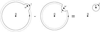
Figure 2: Typical contour deformation for OPE calculations.

There is only one problem with this definition, namely that it involves products of operators. In quantum field theory, this is a notoriously difficult issue. Firstly, operators may not commute, secondly, and more seriously, products of operators at equal points are not well-defined unless normal ordered. As we defined (37), we took care to respect “time” ordering, i.e. radial ordering on the complex plane. In order to evaluate equal-time commutators, we define for operators $A,B$ and arbitrary functions $f,g$ the densities

$$A_{f}=\oint_{0}{\rm d}zf(z)A(z)\,,\ \ \ \ B_{g}=\oint_{0}{\rm d}wg(w)B(w)\,,$$ (38)

where the contours are circles around the origin with radii $|z|=|w|=1$. Then, the equal-time commutator of these objects is

$$[A_{f},B_{g}]_{{\rm e.t.}}=\oint_{C_{1}}{\rm d}zf(z)A(z)\oint_{C_{2}}{\rm d}wg(w)B(w)-\oint_{C_{2}}{\rm d}wg(w)B(w)\oint_{C_{1}}{\rm d}zf(z)A(z)\,,$$ (39)

where we took the freedom to deform the contours in a homologous way such that radial ordering is kept in both terms. As indicated in the figure five, both terms together result in the following expression,

$$[A_{f},B_{g}]_{{\rm e.t.}}=\oint_{0}{\rm d}wg(w)\oint_{w}{\rm d}zf(z)A(z)B(w)$$ (40)

with the contour around $w$ as small as we wish. The inner integration is thus given by the singularities of the operator product expansion (OPE) of $A(z)B(w)$. We suppose that products of operators have an asymptotic expansion for short distances of their arguments. The singular part of this short-distance expansion determines via contour integration the corresponding equal-time commutators. For example, with

$$T_{\varepsilon}=\oint_{0}{\rm d}z\varepsilon(z)T(z)\,,$$ (41)

we recognize immediately $\delta_{\varepsilon}\Phi_{h}(w)=(\varepsilon\partial_{w}+h(\partial_{w}\varepsilon))\Phi_{h}(w)=[T_{\varepsilon},\Phi_{h}(w)]$. Note that this is simply the general version of the common definition of the Virasoro modes $L_{n}=\frac{1}{2\pi{\rm i}}\oint_{0}z^{n+1}T(z)$ for $\varepsilon(z)=z^{n+1}$. If this is to be reproduced by an OPE, it must be of the form

$$T(z)\Phi_{h}(w)=\frac{h}{(z-w)^{2}}\Phi_{h}(w)+\frac{1}{(z-w)}\partial_{w}\Phi_{h}(w)+{\it regular\ terms}\,.$$ (42)

To see this, one essentially has to apply Cauchy’s integral formula $\oint{\rm d}zf(z)(z-w)^{-n}=\frac{1}{(n-1)!}\partial^{n-1}f(w)$. Of course, we may also attempt to find the OPE of the stress-energy tensor with itself from the Virasoro algebra in the same way, which yields

$$T(z)T(w)=\frac{c/2}{(z-w)^{4}}\mbox{$1\!{\rm l}$}+\frac{2}{(z-w)^{2}}T(w)+\frac{1}{(z-w)}\partial_{w}T(w)+{\it regular\ terms}\,.$$ (43)

The reader is encouraged to verify that the above OPE does indeed yield the Virasoro algebra, if substituted into (40).

Note that $T(z)$ is not a proper primary field of weight two due to the term involving the central charge. Since $T(z)$ behaves as a primary field under $L_{i}$, $i\in\{-1,0,1\}$ meaning that it is a weight two tensor with respect to $SL(2,\mathbb{C})$, it is called quasi-primary. One important consequence of this is that the stress-energy tensor on the complex plane and the original stress energy tensor on the cylinder differ by a constant term. Indeed, remembering that the transfer from the complexified cylinder coordinate $w$ to the complex plane coordinate $z$ was given by the conformal map $z={\rm e}^{w}$, one obtains

$$T_{{\rm cyl}}(w)=z^{2}T(z)-\frac{c}{24}\mbox{$1\!{\rm l}$}\,,\ \ \ {\rm i.e.}\ \ \ (L_{n})_{{\rm cyl}}=L_{n}-\frac{c}{24}\delta_{n,0}\,.$$ (44)

This explains the appearance of the factor $-c/24$ in the definition (21) of the Virasoro characters.

The structure of OPEs in CFT is fixed to some degree by two requirements. Firstly, the OPE is not a commutative product, but it should be associative, i.e. $(A(x)B(y))C(z)=A(x)(B(y)C(z))$. The motivation for this presumption comes from the duality properties of string amplitudes. Duality is crossing symmetry in CFT correlation functions, which can be seen to be equivalent to associativity of the OPE. For example, one may evaluate a four-point function in several regions, where different pairs of coordinates are taken close together such that OPEs can be applied. Secondly, the OPE must be consistent with global conformal invariance, i.e. it must respect (17), (18), and (19). This fixes the OPE to be of the following generic form,

$$\Phi_{h_{i}}(z)\Phi_{h_{j}}(w)=\sum_{k}\frac{C_{ij}^{k}}{(z-w)^{h_{i}+h_{j}-h_{k}}}\Phi_{h_{k}}(w)+\ldots\,,$$ (45)

where the structure constants are identical to the structure constants which appeared in the three-point functions (18). Note that due to our normalization of the propagators (two-point functions), raising and lowering of indices is trivial (unless the two-point functions are non-trivial, i.e. $D_{ij}\neq\delta_{ij}$).

• We can divide all fields in a CFT into a few classes. First, there are the primary fields $\Phi_{h}$ corresponding to highest-weight states $|h\rangle$ and second, there are all their Virasoro descendant fields $\Phi_{h}^{(-{\rm\bf n})}$ corresponding to the descendant states $L_{-{\rm\bf n}}|h\rangle$ given by (37). For instance, the stress energy tensor itself is a descendant of the identity, $T(z)=\mbox{$1\!{\rm l}$}^{(-2)}$. We further divide descendant fields into two sub-classes, namely fields which are quasi-primary, and fields which are not. Quasi-primary fields transform conformally covariant for $SL(2,\mathbb{C})$ transformations only.

  General local conformal transformations are implemented in a correlation function by simply inserting the Noether charge, which yields

  $$\delta_{\varepsilon}\langle 0|\Phi_{h_{N}}(z_{N})\ldots\Phi_{h_{1}}(z_{1})|0\rangle=\langle 0|\oint{\rm d}z\varepsilon(z)T(z)\Phi_{h_{N}}(z_{N})\ldots\Phi_{h_{1}}(z_{1})|0\rangle\,,$$ (46)

  where the contour encircles all the coordinates $z_{i}$, $i=1,\ldots,N$. This contour can be deformed into the sum of $N$ small contours, each encircling just one of the coordinates, which is a standard technique in complex analysis. That is equivalent to rewriting (46) as

  $$\sum_{i}\langle 0|\Phi_{h_{N}}(z_{N})\ldots(\delta_{\varepsilon}\Phi_{h_{i}}(z_{i}))\ldots\Phi_{h_{1}}(z_{1})|0\rangle=\sum_{i}\langle 0|\Phi_{h_{N}}(z_{N})\ldots\left(\oint_{z_{i}}{\rm d}z\varepsilon(z)T(z)\Phi_{h_{i}}(z_{i})\right)\ldots\Phi_{h_{1}}(z_{1})|0\rangle\,.$$ (47)

  Since this holds for any $\varepsilon(z)$, we can proceed to a local version of the equality between the right hand sides of (46) and (47), yielding

  $$\langle 0|T(z)\Phi_{h_{N}}(z_{N})\ldots\Phi_{h_{1}}(z_{1})|0\rangle=\sum_{i}\left(\frac{h_{i}}{(z-z_{i})^{2}}+\frac{1}{(z-z_{i})}\partial_{z_{i}}\right)\langle 0|\Phi_{h_{N}}(z_{N})\ldots\Phi_{h_{1}}(z_{1})|0\rangle\,.$$ (48)

  This identity is extremely useful, since it allows us to compute any correlation function involving descendant fields in terms of the corresponding correlation function of primary fields. For the sake of simplicity, let us consider the correlator $\langle 0|\Phi_{h_{N}}(z_{N})\ldots\Phi_{h_{1}}(z_{1})\Phi_{h}^{(-k)}(z)|0\rangle$ with only one descendant field involved. Inserting the definition (37) and using the conformal Ward identity (48), this gives

  $$\oint\frac{{\rm d}w}{(w-z)^{k-1}}$$

  $$\times \left[\langle 0|T(z)\Phi_{h_{N}}(z_{N})\ldots\Phi_{h_{1}}(z_{1})\Phi_{h}(z)|0\rangle-\sum_{i}\left(\frac{h_{i}}{(w-z_{i})^{2}}+\frac{1}{(w-z_{i})}\partial_{z_{i}}\right)\langle 0|\Phi_{h_{N}}(z_{N})\ldots\Phi_{h_{1}}(z_{1})\Phi_{h}(z)|0\rangle\right]\,.$$

  The contour integration in the first term encircles all the coordinates $z$ and $z_{i}$, $i=1,\ldots,N$. Since there are no other sources of poles, we can deform the contour to a circle around infinity by pulling it over the Riemann sphere accordingly. The highest-weight property $\langle 0|L_{k}=0$ for $k\leq 1$ ensures that the integral around $w=\infty$ vanishes. The other terms are evaluated with the help of Cauchy’s formula to

  $${\cal L}_{-k}^{i}\equiv-\oint_{z_{i}}\frac{{\rm d}w}{(w-z)^{k-1}}\left(\frac{h_{i}}{(w-z_{i})^{2}}+\frac{1}{(w-z_{i})}\partial_{z_{i}}\right)=\frac{(k-1)h_{i}}{(z_{i}-z)^{k}}+\frac{1}{(z_{i}-z)^{k-1}}\partial_{z_{i}}\,.$$ (50)

Going through the above small-print shows that a correlation function involving descendant fields can be expressed in terms of the correlation function of the corresponding primary fields only, on which explicitly computable partial differential operators act. Collecting ${\cal L}_{-k}=\sum_{i}{\cal L}_{-k}^{i}$ yields a partial differential operator (which implicitly depends on $z$) such that

$$\langle 0|\Phi_{h_{N}}(z_{N})\ldots\Phi_{h_{1}}(z_{1})\Phi_{h}^{(-k)}(z)|0\rangle={\cal L}_{-k}\langle 0|\Phi_{h_{N}}(z_{N})\ldots\Phi_{h_{1}}(z_{1})\Phi_{h}(z)|0\rangle\,,$$ (51)

where this operator ${\cal L}_{-k}$ has the explicit form

$${\cal L}_{-k}=\sum_{i=1}^{N}\left(\frac{(k-1)h_{i}}{(z_{i}-z)^{k}}+\frac{1}{(z_{i}-z)^{k-1}}\partial_{z_{i}}\right)$$ (52)

for $k>1$. Due to the global conformal Ward identities, the case $k=1$ is much simpler, being just the derivative of the primary field, i.e. ${\cal L}_{-1}=\partial_{z}$. Thus, correlators involving descendant fields are entirely expressed in terms of correlators of primary fields only. Once we know the latter, we can compute all correlation functions of the CFT.

On the other hand, if we use a descendant, which is a null field, i.e.

$$\chi_{h,c}^{(N)}(z)=\sum_{|{\rm\bf n}|=N}\beta^{{\rm\bf n}}\Phi_{h}^{(-{\rm\bf n})}(z)$$ (53)

with $|\chi_{h,c}^{(N)}\rangle$ orthogonal to all other states, we know that it completely decouples from the physical states. Hence, every correlation function involving $\chi_{h,c}^{(N)}(z)$ must vanish. Hence, we can turn things around and use this knowledge to find partial differential equations, which must be satisfied by the correlation function involving the primary $\Phi_{h}(z)$ instead. For example, the level $N=2$ null field yields according to (31) the equation

$$\left({\textstyle\frac{2}{3}}(2h_{\pm}+1){\cal L}_{-2}-\partial_{z}^{2}\right)\langle 0|\Phi_{h_{N}}(z_{N})\ldots\Phi_{h_{1}}(z_{1})\Phi_{h_{\pm}}(z)|0\rangle=0$$ (54)

with $h_{\pm}$ given by the non-trivial values in (30).

A particular interesting case is the four-point function. The three global conformal Ward identities (10) then allow us to express derivatives with respect to $z_{1},z_{2},z_{3}$ in terms of derivatives with respect to $z$. Every new-comer to CFT should once in her life go through this computation for the level two null field: If the field $\Phi_{h}(z)$ is degenerate of level two, i.e. possesses a null field at level two, we can reduce the partial differential equation (54) for $G_{4}=\langle\Phi_{h_{3}}(z_{3})\Phi_{h_{2}}(z_{2})\Phi_{h_{1}}(z_{1})\Phi_{h}(z)\rangle$ to an ordinary Riemann differential equation

$$0 = \left(\frac{3}{2(2h+1)}\partial_{z}^{2}-\sum_{i=1}^{3}\left(\frac{h_{i}}{(z-z_{i})^{2}}+\frac{1}{z-z_{i}}\partial_{z_{i}}\right)\right)G_{4}$$

$$= \left(\frac{3}{2(2h+1)}\partial_{z}^{2}+\sum_{i=1}^{3}\left(\frac{1}{z-z_{i}}\partial_{z}-\frac{h_{i}}{(z-z_{i})^{2}}\right)+\sum_{i<j}\frac{h+h_{i}+h_{j}-\varepsilon_{ij}^{k}h_{k}}{(z-z_{i})(z-z_{j})}\right)G_{4}\,.$$

This can be brought into the well-known form of the Gauss hypergeometric equation by extracting a suitable factor $x^{p}(1-x)^{q}$ from $G_{4}$ with $x$ the crossing ratio $x=\frac{(z-z_{1})(z_{2}-z_{3})}{(z-z_{3})(z_{2}-z_{1})}$. Using the general ansatz (19), we first rewrite the four-point function for the particular choice of coordinates $z_{3}=\infty$, $z_{2}=1$, and $z_{1}=0$ (i.e. $z\equiv x$) in the following form, where we renamed $h=h_{0}$ to allow consistent labeling:

$$\langle\Phi_{h_{3}}(\infty)\Phi_{h_{2}}(1)\Phi_{h_{1}}(0)\Phi_{h_{0}}(z)\rangle = z^{p+\mu_{01}}(1-z)^{q+\mu_{20}}F(z)\,,$$ (56)

$$\mu_{ij} = (h_{0}+h_{1}+h_{2}+h_{3})/3-h_{i}-h_{j}\,,$$

$$p = {\textstyle\frac{1}{6}-\frac{2}{3}h_{0}-\mu_{01}-\frac{1}{6}\sqrt{r_{1}}}\,,$$

$$q = {\textstyle\frac{1}{6}-\frac{2}{3}h_{0}-\mu_{01}-\frac{1}{6}\sqrt{r_{2}}}\,,$$

$$r_{i} = {\textstyle 1-8h_{0}+16h_{0}^{3}+48h_{i}h_{0}+24h_{i}}\,.$$

The remaining function $F(z)$ then is a solution of the hypergeometric system ${}_{2}F_{1}(a,b;c;z)$ given by

$$0 = \left(z(1-z)\partial_{z}^{2}+[c-(a+b+1)z]\partial_{z}-ab\right)F(z)\,,$$ (57)

$$a = {\textstyle\frac{1}{2}-\frac{1}{6}\sqrt{r_{1}}-\frac{1}{6}\sqrt{r_{2}}-\frac{1}{6}\sqrt{r_{3}}}\,,$$

$$b = {\textstyle\frac{1}{2}-\frac{1}{6}\sqrt{r_{1}}-\frac{1}{6}\sqrt{r_{2}}+\frac{1}{6}\sqrt{r_{3}}}\,,$$

$$c = {\textstyle 1-\frac{1}{3}\sqrt{r_{1}}}\,.$$

The general solution is then a linear combination of the two linearly independent solutions ${}_{2}F_{1}(a,b;c;z)$ and $z^{1-c}{}_{2}F_{1}(a-c+1,b-c+1;2-c;z)$. Which linear combination one has to take is determined by the requirement that the full four-point function involving holomorphic and anti-holomorphic dependencies must be single-valued to represent a physical observable quantity. For $|z|<1$, the hypergeometric function enjoys a convergent power series expansion

$${}_{2}F_{1}(a,b;c;z)=\sum_{n=0}^{\infty}\frac{(a)_{n}(b)_{n}}{(c)_{n}}\frac{z^{n}}{n!}\,,\ \ \ \ (x)_{n}=\Gamma(x+n)/\Gamma(x)\,,$$ (58)

but it is a quite interesting point to note that the integral representation has a remarkably similarity to expressions of dual string-amplitudes encountered in string theory, namely

$${}_{2}F_{1}(a,b;c;z)=\frac{\Gamma(c)}{\Gamma(b)\Gamma(c-b)}\int_{0}^{1}{\rm d}t\,t^{b-1}(1-t)^{c-b-1}(1-zt)^{-a}\,,$$ (59)

which, of course, is no accident. However, we must leave this issue to the curiosity of the reader, who might browse through the literature looking for the keyword free field construction.

• A further consequence of the fact, that descendants are entirely determined by their corresponding primaries is that we can refine the structure of OPEs. Let us assume we want to compute the OPE of two primary fields. The right hand side will possibly involve both, primary and descendant fields. Since the coefficients for the descendant fields are fixed by local conformal covariance, we may rewrite (45) as

  $$\Phi_{h_{i}}(z)\Phi_{h_{j}}(w)=\sum_{k,{\rm\bf n}}{\cal C}_{ij}^{k}\beta_{ij}^{k,{\rm\bf n}}\,(z-w)^{h_{k}+|{\rm\bf n}|-h_{i}-h_{j}}\Phi_{h_{k}}^{(-{\rm\bf n})}(w)\,,$$ (60)

  where the coefficients $\beta$ are determined by conformal covariance. Note that we have skipped the anti-holomorphic part, although an OPE is in general only well-defined for fields of the full theory, i.e. for fields $\Phi_{h,\bar{h}}(z,\bar{z})$. An exception is the case where all conformal weights satisfy $2h\in\mathbb{Z}$, since then holomorphic fields are already local.

  Finally, we can explain how associativity of the OPE and crossing symmetry are related. Let us consider a four-point function $G_{ijkl}(z,\bar{z})=\langle 0|\phi_{l}(\infty,\infty)\phi_{k}(1,1)\phi_{j}(z,\bar{z})\phi_{i}(0,0)|0\rangle$. There are three different regions for the free coordinate $z$, for which an OPE makes sense, corresponding to the contractions $z\rightarrow 0:(i,j)(k,l)$, $z\rightarrow 1:(k,j)(i,l)$, and $z\rightarrow\infty:(l,j)(k,i)$. In fact, these three regions correspond to the $s$, $t$, and $u$ channels. Duality states, that the evaluation of the four-point function should not depend on this choice. Absorbing all descendant contributions into functions ${\cal F}$ called conformal blocks, duality imposes the conditions

  $$G_{ijkl}(z,\bar{z}) = \sum_{m}C_{ij}^{m}C_{mkl}{\cal F}_{ijkl}(z|m)\bar{{\cal F}}_{ijkl}(\bar{z}|m)$$

  $$= \sum_{m}C_{jk}^{m}C_{mli}{\cal F}_{ijkl}(1-z|m)\bar{{\cal F}}_{ijkl}(1-\bar{z}|m)$$

  $$= \sum_{m}C_{jl}^{m}C_{mki}z^{-2h_{j}}{\cal F}_{ijkl}({\displaystyle\frac{1}{z}}|m)\bar{z}^{-2\bar{h}_{j}}\bar{{\cal F}}_{ijkl}({\displaystyle\frac{1}{z}}|m)\,,$$

  where $m$ runs over all primary fields which appear on the right hand side of the corresponding OPEs. The careful reader will have noted that these last equations were written down in terms of the full fields in the so-called diagonal theory, i.e. where $\bar{h}=h$ for all fields. This is one possible solution to the physical requirement that the full correlator be a single-valued analytic function. Under certain circumstances, other solutions, so-called non-diagonal theories, do exist.

Figure 3: The three different ways to evaluate a four-point amplitude, i.e. $s$- $t$- and $u$-channels.

• In the full theory, with left- and right-chiral parts combined, the OPE has the following structure, where the contributions from descendants have been made explicit:

  $$\Phi_{h_{i},\bar{h}_{i}}(z,\bar{z})\Phi_{h_{j},\bar{h}_{j}}(w,\bar{w})=\sum_{k,{\rm\bf n}}\sum_{\bar{k},\bar{{\rm\bf n}}}{\cal C}_{ij}^{k}\beta_{ij}^{k,{\rm\bf n}}{\cal C}_{\bar{\imath}\bar{\jmath}}^{\bar{k}}\beta_{\bar{\imath}\bar{\jmath}}^{\bar{k},\bar{{\rm\bf n}}}\,(z-w)^{h_{k}+|{\rm\bf n}|-h_{i}-h_{j}}(\bar{z}-\bar{w})^{\bar{h}_{k}+|\bar{{\rm\bf n}}|-\bar{h}_{i}-\bar{h}_{j}}\Phi_{h_{k},\bar{h}_{k}}^{(-{\rm\bf n},-\bar{{\rm\bf n}})}(w,\bar{w})\,.$$ (62)

  Correlation functions in the full CFT should be single valued in order to represent observables, i.e. physical measurable quantities. This imposes further restrictions on the particular linear combinations of the conformal blocks ${\cal F}_{ijkl}(z|m)$ in (2.4). In most CFTs, the diagonal combination $\bar{h}=h$ is a solution, but it is easy to see, that the monodromy of a field $\Phi_{h,\bar{h}}(z,\bar{z})$ under $z\mapsto{\rm e}^{2\pi{\rm i}}z$ yields the less restrictive condition $h-\bar{h}\in\mathbb{Z}$, such that off-diagonal solutions can be possible.

  The success story of CFT is much rooted in the following observation first made by Belavin, Polyakov and Zamolodchikov [2]: If an OPE of two primary fields $\Phi_{i}(z)\Phi_{j}(w)$ is considered, which both are degenerated at levels $N_{i}$ and $N_{j}$ respectively, then the right hand side will only involve contributions from primary fields, which all are degenerate at a certain levels $N_{k}\leq N_{i}+N_{j}$. In particular, the sum over conformal families $k$ on the right hand side is then always finite, and so is the set of conformal blocks one has to know. In particular, the set of degenerate primary fields (and their descendants) forms a closed operator algebra. For example, considering a four-point function where all four fields are degenerate at level two, we find only two conformal blocks for each channel, which precisely are the hypergeometric functions computed above and their analytic continuations. Even more remarkably, for the special values $c(m)$ in (32) with $m\in\mathbb{N}$, there are only finitely many primary fields with conformal weights $h_{p,q}(c)$ with $1\leq p<m$ and $1\leq q<m+1$ given by(2.3). All other degenerate primary fields with weights $h_{p,q}(c)$ where $p$ or $q$ lie outside this range turn out to be null fields within the Verma modules of the descendants of these former primary fields. Hence, such CFTs have a finite field content and are actually the “smallest” CFTs. This is why they are called minimal models. Unfortunately, they are not very useful for string theory, but turn up in many applications of statistical physics [55].

3 Logarithmic null vectors

We have learned in the basic introductionary lectures that logarithmic conformal field theory (LCFT) arises due to the existence of indecomposable representations. Thus, instead of a unique highest weight state, on which the representation module is built, we have to deal with a Jordan cell of states which are linked by the action of some operator which cannot be diagonalized. In most cases, this will be the action of the stress-energy tensor, but in general Jordan cells might occur due to the action of any generator of the (extended) chiral symmetry algebra. To keep things simple, we will confine ourselves to the Virasoro case within these notes. We will see other examples in the lectures by Matthias Gaberdiel.

Let us briefly recall what we mean by Jordan cell structure. Suppose we have two operators $\Phi(z),\Psi(z)$ with the same conformal weight $h$, or more precisely, with an equivalent set of quantum numbers with respect to the maximally extended chiral symmetry algebra. As was first realized in [48], this situation leads to logarithmic correlation functions and to the fact that $L_{0}$, the zero mode of the Virasoro algebra, can no longer be diagonalized:

$$L_{0}|{\Phi}\rangle = h|{\Phi}\rangle\,,$$

$$L_{0}|{\Psi}\rangle = h|{\Psi}\rangle+|{\Phi}\rangle\,,$$ (63)

where we worked with states instead of the fields themselves. The field $\Phi(z)$ is then an ordinary primary field, whereas the field $\Psi(z)$ gives rise to logarithmic correlation functions and is therefore called a logarithmic partner of the primary field $\Phi(z)$. We would like to note once more that two fields of the same conformal dimension do not automatically lead to LCFTs with respect to the Virasoro algebra. Either, they differ in some other quantum numbers (for examples of such CFTs see [32]), or they form a Jordan cell structure with respect to an extended chiral symmetry only (see [71] for a description of the different possible cases).

We remember that a singular or null vector $|{\chi}\rangle$ is a state which is orthogonal to all states,

$$\langle{\psi}|{\chi}\rangle=0\ \forall|{\psi}\rangle\,,$$ (64)

where the scalar product is given by the Shapovalov form. Such states can be considered to be identically zero.

A pair of fields $\Phi(z),\Psi(z)$ forming a Jordan cell structure brings the problem of off-diagonal terms produced by the action of the Virasoro field, such that the corresponding representation is indecomposable. Therefore, if $\left|{\chi_{\Phi}}\right\rangle$ is a null vector in the Verma module on the highest weight state $|{\Phi}\rangle$ of the primary field, we cannot just replace $|{\Phi}\rangle$ by $|{\Psi}\rangle$ and obtain another null vector.

Before we define general null vectors for Jordan cell structures, we present a formalism which might be useful in the future for all kinds of explicit calculations in the LCFT setting. This formalism, has the advantage that the Virasoro modes are still represented as linear differential operators, and that it is compact and elegant allowing for arbitrary rank Jordan cell structures. Moreover, the connection between LCFTs and supersymmetric CFTs, which one could glimpse here and there [16, 33, 105, 106] (see also [22]), seems to be a quite fundamental one.

3.1 Jordan cells and nilpotent variable formalism

LCFTs are characterized by the fact that some of their highest weight representations are indecomposable. This is usually described by saying that two (or more) highest weight states with the same highest weight span a non-trivial Jordan cell. In the following we call the dimension of such a Jordan cell the rank of the indecomposable representation.

Therefore, let us assume that a given LCFT has an indecomposable representation of rank $r$ with respect to its maximally extended chiral symmetry algebra ${\cal W}$. This Jordan cell is spanned by $r$ states $|{w_{0},w_{1},\ldots;n}\rangle$, $n=0,\ldots,r-1$ such that the modes of the generators of the chiral symmetry algebra act as

$$\Phi^{(i)}_{0}|{w_{0},w_{1},\ldots;n}\rangle = w_{i}|{w_{0},w_{1},\ldots;n}\rangle+\sum_{k=0}^{n-1}a_{i,k}|{w_{0},w_{1},\ldots;k}\rangle\,,$$ (65)

$$\Phi^{(i)}_{m}|{w_{0},w_{1},\ldots;n}\rangle = 0\ {\rm for}\ m>0\,,$$ (66)

where usually $\Phi^{(0)}(z)=T(z)$ is the stress energy tensor which gives rise to the Virasoro field, i.e. $\Phi^{(0)}_{0}=L_{0}$, and $w_{0}=h$ is the conformal weight. For the sake of simplicity, we concentrate in these notes on the representation theory of LCFTs with respect to the pure Virasoro algebra such that (65) reduces to

$$L_{0}|{h;n}\rangle = h|{h;n}\rangle+(1-\delta_{n,0})|{h;n-1}\rangle\,,$$ (67)

$$L_{m}|{h;n}\rangle = 0\ {\rm for}\ m>0\,,$$ (68)

where we have normalized the off-diagonal contribution to 1. As in ordinary CFTs, we have an isomorphism between states and fields. Thus, the state $|{h;0}\rangle$, which is the highest weight state of the irreducible sub-representation contained in every Jordan cell, corresponds to an ordinary primary field $\Psi_{(h;0)}(z)\equiv\Phi_{h}(z)$, whereas states $|{h;n}\rangle$ with $n>0$ correspond to the so-called logarithmic partners $\Psi_{(h;n)}(z)$ of the primary field. The action of the modes of the Virasoro field on these primary fields and their logarithmic partners is given by

$${\cal L}_{-k}(z)\Psi_{(h;n)}(w)=$$

$$\frac{(1-k)h}{(z-w)^{k}}\Psi_{(h;n)}(w)-\frac{1}{(z-w)^{k-1}}\frac{\partial}{\partial w}\Psi_{(h;n)}(w)-(1-\delta_{n,0})\frac{\lambda(1-k)}{(z-w)^{k}}\Psi_{(h;n-1)}(w)\,,$$

with $\lambda$ normalized to 1 in the following. As it stands, the off-diagonal term spoils writing the modes ${\cal L}_{-k}(z)$ as linear differential operators.

• There is one subtlety here. In these notes we assume that the logarithmic partner fields of a primary field are all quasi-primary in the sense that the corresponding states $|{h;n}\rangle$ are all annihilated by the action of modes $L_{m}$, $m>0$. This is not necessarily the case, and there are examples of LCFTs where Jordan blocks occur, where the logarithmic partner is not quasi-primary. For instance, the Jordan block of $h=1$ fields in the $c=-2$ LCFT is made up of a primary field with highest weight state $|{\phi}\rangle$ and a logarithmic partner $|{\psi}\rangle$ such that

  $$L_{0}|{\phi}\rangle=|{\phi}\rangle\,,\ \ \ \ L_{0}|{\psi}\rangle=|{\psi}\rangle+|{\phi}\rangle\,,\ \ \ \ L_{1}|{\phi}\rangle=0\,,\ \ \ \ L_{1}|{\psi}\rangle=|{\xi}\rangle\,,$$

  where $|{\xi}\rangle$, a state corresponding to a field of zero conformal weight, is related to the primary field via $L_{-1}|{\xi}\rangle=|{\phi}\rangle$. Note that in this particular example, the primary field corresponding to $|{\phi}\rangle$ is a current, and a descendant of the field corresponding to $|{\xi}\rangle$. However, there are indications that such indecomposable representations with non-quasi-primary states of weight $h$ only occur together with a corresponding indecomposable representation of only quasi-primary states of weight $h-k$, $k\in\mathbb{Z}_{+}$. We are not going to investigate this issue further, but note that all so far explicitly known LCFTs possess at least one indecomposable representation where all states of the basic Jordan block are quasi-primary. Since it is a very difficult task to construct null vectors on non-quasi-primary states, we will not consider such indecomposable representations here. For more details on the issue of Jordan cells with non-quasi-primary fields see the last reference in [33].

Our first aim is simply to prepare a formalism in which the Virasoro modes are expressed as linear differential operators. To this end, we introduce a new – up to now purely formal – variable $\theta$ with the property $\theta^{r}=0$. We may then view an arbitrary state in the Jordan cell, i.e. a particular linear combination

$$\Psi_{h}({\rm\bf a})(z)=\sum_{n=0}^{r-1}a_{n}\Psi_{(h;n)}(z)\,,$$ (70)

as a formal series expansion describing an arbitrary function $a(\theta)$ in $\theta$, namely

$$\Psi_{h}(a(\theta))(z)=\sum_{n}a_{n}\frac{\theta^{n}}{n!}\Psi_{h}(z)\,.$$ (71)

This means that the space of all states in a Jordan cell can be described by tensoring the primary state with the space of power series in $\theta$, i.e. $\Theta_{r}(\Psi_{h})\equiv\Psi_{h}(z)\otimes\mathbb{C}[\![\theta]\!]/{\cal I}$, where we divided out the ideal generated by the relation ${\cal I}=\langle\theta^{r}\!=\!0\rangle$. In fact, the action of the Virasoro algebra is now simply given by

$${\cal L}_{-k}(z)\Psi_{h}(a(\theta))(w)=\left(\frac{(1-k)h}{(z-w)^{k}}-\frac{1}{(z-w)^{k-1}}\frac{\partial}{\partial w}-\frac{\lambda(1-k)}{(z-w)^{k}}\frac{\partial}{\partial\theta}\right)\Psi_{h}(a(\theta))(w)\,.$$ (72)

Clearly, $\Psi_{(h;n)}(z)=\Psi_{h}(\theta^{n}/n!)(z)$, but we will often simplify notation and just write $\Psi_{h}(\theta)(z)$ for a generic element in $\Theta_{r}(\Psi_{h})$. However, the context should always make it clear, whether we mean a generic element or really $\Psi_{(h;1)}(z)$. The corresponding states are denoted by $|{h;a(\theta)}\rangle$ or simply $|{h;\theta}\rangle$. To project onto the $k^{{\rm th}}$ highest weight state of the Jordan cell, we just use $a_{k}|{h;k}\rangle=\left.\partial_{\theta}^{k}|{h;a(\theta)}\rangle\right|_{\theta=0}$. In order to avoid confusion with $|{h;1}\rangle$ we write $|{h;\mathbb{I}}\rangle$ if the function $a(\theta)\equiv 1$.

It has become apparent by now that LCFTs are somehow closely linked to supersymmetric CFTs [16, 33, 105, 106] (see also [22]). We suggestively denoted our formal variable by $\theta$, since it can easily be constructed with the help of Grassmannian variables as they appear in supersymmetry. Taking $N\!=\!r-1$ supersymmetry with Grassmann variables $\theta_{i}$ subject to $\theta_{i}^{2}=0$, we may define $\theta=\sum_{i=1}^{r-1}\theta_{i}$. More generally, $\theta$ and its powers constitute a basis of the totally symmetric, homogenous polynomials in the Grassmannians $\theta_{i}$.

Finally, we remark that the $\theta$ variables are associated not with the coordinates the fields are localized in coordinate space, but with the positions the fields are localized in $h$-space (the Jordan cells). Therefore, the $\theta$ variables will be labeled by the conformal weight they refer to, whenever the context makes it necessary.

3.2 Logarithmic null vectors

Next, we derive the consequences of our formalism. An arbitrary state in a LCFT of level $n$ is a linear combination of descendants of the form

$$|{\psi(\theta)}\rangle=\sum_{k}\sum_{\{n_{1}+n_{2}+\ldots+n_{m}=n\}}b^{\{n_{1},n_{2},\ldots,n_{m}\}}_{k}L_{-n_{m}}\ldots L_{-n_{2}}L_{-n_{1}}|{h;k}\rangle$$ (73)

which we often abbreviate as

$$|{\psi(\theta)}\rangle=\sum_{|{\rm\bf n}|=n}L_{-{\rm\bf n}}b^{{\rm\bf n}}(\theta)|{h}\rangle\,.$$ (74)

We will mainly be concerned with calculating Shapovalov forms $\langle{\psi^{\prime}(\theta^{\prime})}|{\psi(\theta)}\rangle$ which ultimately cook down (by commuting Virasoro modes through) to expressions of the form

$$\langle{\psi^{\prime}(\theta^{\prime})}|{\psi(\theta)}\rangle=\langle{h^{\prime};a^{\prime}(\theta^{\prime})}|\sum_{m}f_{m}(c)(L_{0})^{m}|{h;a(\theta)}\rangle\,,$$ (75)

where we explicitly noted the dependence of the coefficients on the central charge $c$. Combining (75) with (74) we write $\langle{\psi^{\prime}(\theta^{\prime})}|{\psi(\theta)}\rangle=\langle{h^{\prime};a^{\prime}(\theta^{\prime})}|f_{{\rm\bf n}^{\prime},{\rm\bf n}}(L_{0},C)|{h;a(\theta)}\rangle$ for the Shapovalov form between two monomial descendants, i.e.

$$\langle{h^{\prime};a^{\prime}(\theta^{\prime})}|f_{{\rm\bf n}^{\prime},{\rm\bf n}}(L_{0},C)|{h;a(\theta)}\rangle=\langle{h^{\prime};a^{\prime}(\theta^{\prime})}|L_{n^{\prime}_{1}}L_{n^{\prime}_{2}}\ldots L_{-n_{2}}L_{-n_{1}}|{h;a(\theta)}\rangle\,.$$ (76)

More generally, since $L_{0}|{h;a(\theta)}\rangle=(h+\partial_{\theta})|{h;a(\theta)}\rangle$, it is easy to see that an arbitrary function $f(L_{0},C)\in\mathbb{C}[\![L_{0},C]\!]$ acts as

$$f(L_{0},C)|{h;n}\rangle=\sum_{k}\frac{1}{k!}\left(\frac{\partial^{k}}{\partial h^{k}}f(h,c)\right)|{h;n-k}\rangle\,,$$ (77)

and therefore $f(L_{0},C)|{h;a(\theta)}\rangle=|{h;\tilde{a}(\theta)}\rangle$, where with $a(\theta)=\sum_{n}a_{n}\frac{\theta^{n}}{n!}$ we have

$$\tilde{a}_{n}=\sum_{k}\frac{a_{n+k}}{k!}\frac{\partial^{k}}{\partial h^{k}}f(h,c)\,.$$ (78)

• It may be instructive to check this statement explicitly for the simple case $f(L_{0},C)=L_{0}^{m}$. Keeping in mind that $|{h;n}\rangle=|{h;\frac{1}{n!}\theta^{n}}\rangle$, one then finds

  $$L_{0}^{m}|{h;n}\rangle = (h+\partial_{\theta})^{m}|{h;\frac{1}{n!}\theta^{n}}\rangle=\sum_{k}{m\choose k}h^{m-k}\partial_{\theta}^{k}|{h;\frac{1}{n!}\theta^{n}}\rangle=\sum_{k}{m\choose k}h^{m-k}\frac{n(n-1)\ldots(n-k+1)}{n!}|{h;\theta^{n-k}}\rangle$$ (79)

  $$= \sum_{k}\frac{m!}{k!(m-k)!}\frac{1}{(n-k)!}h^{m-k}|{h;\theta^{n-k}}\rangle=\sum_{k}\frac{1}{k!}m(m-1)\ldots(m-k+1)h^{k}|{h;n-k}\rangle$$

  $$= \sum_{k}\frac{1}{k!}(\partial_{h}^{k}h^{m})|{h;n-k}\rangle=\sum_{k}\frac{1}{k!}\partial_{h}^{k}f(h,c)|{h;n-k}\rangle\,.$$

  Since more general functions $f(L_{0},C)$ are merely linear combinations of the above example with different $m$, the general statement should be clear. Note, however, that sofar the central charge only enters as an external parameter.

This puts the convenient way of expressing the action of $L_{0}$ on Jordan cells by derivatives with respect to the conformal weight $h$, which appeared earlier in the literature, on a firm ground. Moreover, from now on we do not worry about the range of summations, since all series automatically truncate in the right way due to the condition $\theta^{r}=0$.

It is evident that choosing $a(\theta)=\mathbb{I}$ extracts the irreducible sub-representation which is invariant under the action of $L_{0}$. All other non-trivial choices of $a(\theta)$ yield states which are not invariant under the action of $L_{0}$. The existence of null vectors of level $n$ on such a particular state is subject to the conditions that

$$\sum_{|{\rm\bf n}|=n}f_{{\rm\bf n}^{\prime},{\rm\bf n}}(L_{0},C)b^{{\rm\bf n}}(\theta,h,c)|{h}\rangle$$

$$\equiv \sum_{|{\rm\bf n}|=n}f_{{\rm\bf n}^{\prime},{\rm\bf n}}(L_{0},C)\sum_{k}b^{{\rm\bf n}}_{k}(h,c)|{h;k}\rangle=0\ \ \ \ \forall\ {\rm\bf n}^{\prime}:|{\rm\bf n}^{\prime}|=n\,.$$

Notice that we have the freedom that each highest weight state of the Jordan cell comes with its own descendants. These conditions determine the $b^{{\rm\bf n}}_{k}(h,c)$ as functions in the conformal weight and the central charge. Clearly, for $a(\theta)=\mathbb{I}$ this would just yield the ordinary results as known since BPZ [2], i.e. the solutions for $b^{{\rm\bf n}}_{0}(h,c)$. The question is now, under which circumstances null vectors exist on the whole Jordan cell, i.e. for non-trivial choices of $a(\theta)$. Obviously, these null vectors, which we call logarithmic null vectors can only constitute a subset of the ordinary null vectors. From (77) we immediately learn that the conditions imply

$$\sum_{k=0}^{s-1}\sum_{|{\rm\bf n}|=n}b^{{\rm\bf n}}_{k}(h,c)\frac{1}{(s-1-k)!}\frac{\partial^{s-1-k}}{\partial h^{s-1-k}}f_{{\rm\bf n}^{\prime},{\rm\bf n}}(h,c)=0\ \ \forall\ {\rm\bf n}^{\prime}:|{\rm\bf n}^{\prime}|=n\,,\ 1\leq s\leq r\,.$$ (81)

• To see this, simply start with $s=1$ and observe that this recovers the well known condition for a generic null vector of a ordinary non-logarithmic CFT, $\sum_{|{\rm\bf n}|=n}b_{0}^{{\rm\bf n}}(h,c)f_{{\rm\bf n}^{\prime},{\rm\bf n}}(h,c)=0$. Then proceed inductively. In the next step, $s=2$, one now finds a condition which relates the coefficients $b_{1}^{{\rm\bf n}}(h,c)$ and the coefficients $b_{0}^{{\rm\bf n}}(h,c)$,

  $$\sum_{|{\rm\bf n}|=n}\left(b_{1}^{{\rm\bf n}}(h,c)f_{{\rm\bf n}^{\prime},{\rm\bf n}}(h,c)+b_{0}^{{\rm\bf n}}(h,c)\partial_{h}f_{{\rm\bf n}^{\prime},{\rm\bf n}}(h,c)\right)=0\,,$$

  which is clear since the action of $L_{0}$ on $|{h;1}\rangle$ will produce terms proportional to $|{h;0}\rangle$. Since $L_{0}$ never moves up within a Jordan block, the condition for the coefficients for $|{h;s-1}\rangle$ can only involve the coefficients for states $|{h;s^{\prime}-1}\rangle$, $0\leq s^{\prime}<s$. Thus, we arrive at the above statement.

The conditions (81) can be satisfied if we put

$$b^{{\rm\bf n}}_{k}(h,c)=\frac{1}{k!}\frac{\partial^{k}}{\partial h^{k}}b^{{\rm\bf n}}_{0}(h,c)\,.$$ (82)

In fact, choosing the $b^{{\rm\bf n}}_{k}(h,c)$ in this way allows one to rewrite the conditions as total derivatives of the standard condition for $b^{{\rm\bf n}}_{0}(h,c)$. Keeping in mind that each Jordan cell module of rank $r$ has Jordan cells of ranks $r^{\prime}$, $1\leq r^{\prime}\leq r$, as submodules, we can find intermediate null vector conditions, where the null vector only lies in the rank $r^{\prime}$ submodule (think of $r^{\prime}=1$ as a trivial example), if we restrict the range of $s$ in (81) accordingly. Of course, this determines the $b^{{\rm\bf n}}_{k}(h,c)$ only up to terms of lower order in the derivatives such that the conditions finally take the general form

$$\sum_{k}\frac{\lambda_{k}}{k!}\frac{\partial^{k}}{\partial h^{k}}\left(\sum_{|{\rm\bf n}|=n}f_{{\rm\bf n}^{\prime},{\rm\bf n}}(h,c)b^{{\rm\bf n}}_{0}(h,c)\right)=0\ \forall\ {\rm\bf n}^{\prime}:|{\rm\bf n}^{\prime}|=n\,,$$ (83)

which, however, does not yield any different results. Moreover, the coefficients $b^{{\rm\bf n}}_{k}(h,c)$ can only be determined up to an overall normalization. Clearly, there are $p(n)$ coefficients, where $p(n)$ denotes the number of partitions of $n$ into positive integers. This means that only $p(n)-1$ of the standard coefficients $b^{{\rm\bf n}}_{0}(h,c)$ are determined to be functions in $h,c$ multiplied by the remaining coefficient, e.g. $b^{\{1,1,\ldots,1\}}_{0}$ (if this coefficient is not predetermined to vanish). In order to be able to write the coefficients $b^{{\rm\bf n}}_{k}(h,c)$ with $k>0$ as derivatives with respect to $h$, one needs to fix the remaining free coefficient $b^{\{1,1,\ldots,1\}}_{0}=h^{p(n)}$ as a function of $h$. The choice given here ensures that all coefficients are always of sufficient high degree in $h$. Clearly, this works only for $h\neq 0$. To find null vectors with $h=0$ needs some extra care. One foolproof choice is to put the remaining free coefficient to $\exp(h)$. The problem is that the Hilbert space of states is a projective space due to the freedom of normalization, and that we used $h$ as a projective coordinate in this space, which only works for $h\neq 0$.

It is important to understand that the above is only a necessary condition due to the following subtlety: The derivatives with respect to $h$ are done in a purely formal way. But already determining the standard solution $b^{{\rm\bf n}}_{0}(h,c)$ is not sufficient in itself, and the conditions for the existence of standard null vectors yield one more constraint, namely $h=h_{i}(c)$ or vice versa $c=c_{i}(h)$ (the index $i$ denotes possible different solutions, since the resulting equations are higher degree polynomials $\in\mathbb{C}[h,c]$). These constraints must be plugged in after performing the derivatives and, as it will turn out, this will severely restrict the existence of logarithmic null vectors, yielding only some discrete pairs $(h,c)$ for each level $n$. Moreover, the set of solutions gets rapidly smaller if for a given level $n$ the rank $r$ of the assumed Jordan cell is increased. Since there are $p(n)$ linearly independent conditions for the $b^{{\rm\bf n}}_{0}(h,c)$ of a standard null vector of level $n$, a necessary condition is $r\leq p(n)$. As mentioned above, $h$ is not a good coordinate for $h=0$, but $c_{i}(h)$ still is. Therefore, for $h=0$ we should use $c$ for normalization, meaning that for $h=0$, the $c_{i}(h)$ have to be plugged in before doing the derivatives.

3.3 An example

Now we will go through a rather elaborate example to see how all this is supposed to work. So, we are going to demonstrate what a logarithmic null vector is and under which conditions it exists. Null vectors are of particular importance for rational CFTs. For any CFT given by its maximally extended symmetry algebra ${\cal W}$ and a value $c$ for the central charge we can determine the so-called degenerate ${\cal W}$-conformal families which contain at least one null vector. The corresponding highest weights turn out to be parametrized by certain integer labels, yielding the so-called Kac-table. If ${\cal W}=\{T(z)\}$ is just the Virasoro algebra, all degenerate conformal families have highest weights labeled by two integers $r,s$,

$$h_{r,s}(c)=\frac{1}{4}\left(\frac{1}{24}\left(\sqrt{(1-c)}(r+s)-\sqrt{(25-c)}(r-s)\right)^{2}-\frac{1-c}{6}\right)\,.$$ (84)

The level of the (first) null vector contained in the conformal families over the highest weight state $|{h_{r,s}(c)}\rangle$ is then $n=rs$.

LCFTs have the special property that there are at least two conformal families with the same highest weight state, i.e. that we must have $h=h_{r,s}(c)=h_{t,u}(c)$. This does not happen for the so-called minimal models since their truncated conformal grid precisely excludes this. However, LCFTs may be constructed for example for $c=c_{p,1}$, where formally the conformal grid is empty, or by augmenting the field content of a CFT by considering an enlarged conformal grid. However, if we have the situation typical for a LCFT, we have two non-trivial and different null vectors, one at level $n=rs$ and one at $n^{\prime}=tu$ where we assume without loss of generality $n\leq n^{\prime}$. Then the null vector at level $n$ is an ordinary null vector on the highest weight state of the irreducible sub-representation $|{h;0}\rangle$ of the rank 2 Jordan cell spanned by $|{h;0}\rangle$ and $|{h;1}\rangle$, but what about the null vector at level $n^{\prime}$?

Let us consider the particular LCFT with $c=c_{3,1}=-7$. This LCFT admits the highest weights $h\in\{0,\frac{-1}{4},\frac{-1}{3},\frac{5}{12},1,\frac{7}{4}\}$ which yield the two irreducible representations at $h_{1,3}=\frac{-1}{3}$ and $h_{1,6}=\frac{5}{12}$ as well as two indecomposable representations with so-called staggered module structure (roughly a generalization of Jordan cells to the case that some highest weights differ by integers [41, 104]) constituted by the triplets $(h_{1,1}\!=\!0,h_{1,5}\!=\!0,h_{1,7}\!=\!1)$ and $(h_{1,2}\!=\!\frac{-1}{4},h_{1,4}\!=\!\frac{-1}{4},h_{1,8}\!=\!\frac{7}{4})$. We note that similar to the case of minimal models we have the identification $h_{1,s}=h_{2,9-s}$ such that the actual level of the null vector might be reduced. In the following we will determine the null vectors at level 2 and 4 for the rank 2 Jordan cell with $h=\frac{-1}{4}$. First, we start with the level 2 null vector, whose general ansatz is

$$|{\chi^{(2)}_{h,c}}\rangle=\left(b^{\{1,1\}}_{0}L_{-1}^{2}+b^{\{2\}}_{0}L_{-2}\right)|{h;a(\theta)}\rangle+\left(b^{\{1,1\}}_{1}L_{-1}^{2}+b^{\{2\}}_{1}L_{-2}\right)|{h;\partial_{\theta}a(\theta)}\rangle\,,$$ (85)

where we explicitly made clear how we counteract the off-diagonal action of the Virasoro null mode.

• For null vectors of level $n>1$ we make the general ansatz

  $$|{\chi^{(n)}_{h,c}}\rangle=\sum_{j}\sum_{|{\rm\bf n}|=n}b^{{\rm\bf n}}_{j}(h,c)L_{-{\rm\bf n}}\left|{h;\partial_{\theta}^{j}a(\theta)}\right\rangle$$ (86)

  and define matrix elements

  $$N_{k,l}^{(n)} = \left.\frac{\partial^{k}}{\partial\theta^{k}}\left(\sum_{j}\sum_{|{\rm\bf n}|=n}b^{{\rm\bf n}}_{j}(h,c)\left\langle{h}\left|L_{{\rm\bf n}^{\prime}_{l}}L_{-{\rm\bf n}}\left|{h;\partial_{\theta}^{j}a(\theta)}\right\rangle\right.\right.\right)\right|_{\theta=0}$$ (87)

  $$= \sum_{j=0}^{k}\sum_{|{\rm\bf n}|=n}b^{{\rm\bf n}}_{j}(h,c)\frac{1}{j!}\frac{\partial^{j}}{\partial h^{j}}\left\langle{h}\right|L_{{\rm\bf n}^{\prime}_{l}}L_{-{\rm\bf n}}\left|{h}\right\rangle\,,$$

  where ${\rm\bf n}^{\prime}_{l}$ is some enumeration of the $p(n)$ different partitions of $n$. Since the maximal possible rank of a Jordan cell representation which may contain a logarithmic null vector is $r\leq p(n)$, we consider $N^{(n)}$ to be a $p(n)\times p(n)$ square matrix. Our particular ansatz is conveniently chosen to simplify the action of the Virasoro modes on Jordan cells. Notice, that the derivatives with respect to the conformal weight $h$ do not act on the coefficients $b^{{\rm\bf n}}_{j}(h,c)$. Of course, we assume that $a(\theta)$ has maximal degree in $\theta$, i.e. ${\rm deg}(a(\theta))=r-1$.

  In our example at level 2, we have $p(2)=2$ and the matrix $N^{(2)}$ we have to evaluate is

  $$N^{(2)}=\left[\begin{array}[]{cc}b^{\{1,1\}}_{0}\langle{h}|L_{1}^{2}L_{-1}^{2}|{h}\rangle+b^{\{2\}}_{0}\langle{h}|L_{1}^{2}L_{-2}|{h}\rangle&\ \ b^{\{1,1\}}_{0}\partial_{h}\langle{h}|L_{1}^{2}L_{-1}^{2}|{h}\rangle+b^{\{2\}}_{0}\partial_{h}\langle{h}|L_{1}^{2}L_{-2}|{h}\rangle\\ &\ \ {}+b^{\{1,1\}}_{1}\langle{h}|L_{1}^{2}L_{-1}^{2}|{h}\rangle+b^{\{2\}}_{1}\langle{h}|L_{1}^{2}L_{-2}|{h}\rangle\\ \vskip 6.0pt plus 2.0pt minus 2.0pt\cr b^{\{1,1\}}_{0}\langle{h}|L_{2}L_{-1}^{2}|{h}\rangle+b^{\{2\}}_{0}\langle{h}|L_{2}L_{-2}|{h}\rangle&\ \ b^{\{1,1\}}_{0}\partial_{h}\langle{h}|L_{2}L_{-1}^{2}|{h}\rangle+b^{\{2\}}_{0}\partial_{h}\langle{h}|L_{2}L_{-2}|{h}\rangle\\ &\ \ {}+b^{\{1,1\}}_{1}\langle{h}|L_{2}L_{-1}^{2}|{h}\rangle+b^{\{2\}}_{1}\langle{h}|L_{2}L_{-2}|{h}\rangle\end{array}\right]\,.$$ (88)

  Doing the computations, this reads

  $$N^{(2)}=\left[\begin{array}[]{cc}b^{\{1,1\}}_{0}\left(8h^{2}+4h\right)+6b^{\{2\}}_{0}h&b^{\{1,1\}}_{0}\left(16h+4\right)+6b^{\{2\}}_{0}+b^{\{1,1\}}_{1}\left(8h^{2}+4h\right)+6b^{\{2\}}_{1}h\\ \vskip 6.0pt plus 2.0pt minus 2.0pt\cr 6b^{\{1,1\}}_{0}h+b^{\{2\}}_{0}\left(4h+{\textstyle\frac{1}{2}}c\right)&6b^{\{1,1\}}_{0}+4b^{\{2\}}_{0}+6b^{\{1,1\}}_{1}h+b^{\{2\}}_{1}\left(4h+{\textstyle\frac{1}{2}}c\right)\end{array}\right]\,.$$ (89)

  A null vector is logarithmic of rank $k\geq 0$ if the first $k+1$ columns of $N^{(n)}$ are zero, where $k=0$ means an ordinary null vector. As described in the text, one first solves for ordinary null vectors (such that the first column vanishes up to one entry). This determines the $b^{{\rm\bf n}}_{0}(h,c)$. Then one puts $b^{{\rm\bf n}}_{k}(h,c)=\frac{1}{k!}\partial_{h}^{k}b^{{\rm\bf n}}_{0}(h,c)$. Without loss of generality we may then assume that all entries except the last row are zero. In our example, this procedure results in

  $$N^{(2)}=\left[\begin{array}[]{cc}0&0\\ \vskip 6.0pt plus 2.0pt minus 2.0pt\cr 10h^{2}-16h^{3}-2h^{2}c-hc&20h-48h^{2}-4hc-c\end{array}\right]\,,$$ (90)

  where $b^{\{1,1\}}_{k}=\frac{1}{k!}\partial_{h}^{k}(3h)$ and $b^{\{2\}}_{k}=\frac{1}{k!}\partial_{h}^{k}(-2h(2h+1))$ upto an overall normalization. The last step is trying to find simultaneous solutions for the last row, i.e. common zeros of polynomials $\in\mathbb{C}[h,c]$. In our example, $N^{(2)}_{2,1}=0$ yields $c=2h(5-8h)/(2h+1)$. Then, the last condition becomes $N^{(2)}_{2,2}=-2h(16h^{2}+16h-5)/(2h+1)=0$ which can be satisfied for $h\in\{0,\frac{-5}{4},\frac{1}{4}\}$. From this we finally obtain the explicit logarithmic null vectors at level 2:

  $$\begin{array}[]{c|c}(h,c)&|{\chi^{(2)}_{h,c}}\rangle\\ \vskip 3.0pt plus 1.0pt minus 1.0pt\cr\hline\cr\hline\cr\vskip 3.0pt plus 1.0pt minus 1.0pt\cr(0,0)&(3L_{-1}^{2}-2L_{-2})\left|{0;a(\theta)}\right\rangle\\ \vskip 3.0pt plus 1.0pt minus 1.0pt\cr(\frac{1}{4},1)&(3L_{-1}^{2}-3L_{-2})\left|{\frac{1}{4};a(\theta)}\right\rangle-4L_{-2}\left|{\frac{1}{4};\partial_{\theta}a(\theta)}\right\rangle\\ \vskip 3.0pt plus 1.0pt minus 1.0pt\cr(\frac{-5}{4},25)&(3L_{-1}^{2}+3L_{-2})\left|{\frac{-5}{4};a(\theta)}\right\rangle-4L_{-2}\left|{\frac{-5}{4};\partial_{\theta}a(\theta)}\right\rangle\end{array}$$

  Note, that according to our formalism, $h=0,c=0$ does not turn out to be a logarithmic null vector at level 2. Here and in the following the highest order derivative $\partial_{\theta}^{k}a(\theta)$ indicates the maximal rank of a logarithmic null vector to be $k$ (and hence the maximal rank of the corresponding Jordan cell representation to be $r=k+1$). It is implicitly understood that $a(\theta)$ is then chosen such that the highest order derivative yields a non-vanishing constant.

  Here, all null vectors are normalized such that all coefficients are integers. Clearly, they are not unique since with $\left|{\chi(\theta)}\right\rangle=\sum_{k}\left|{\chi_{k};\partial_{\theta}^{k}a(\theta)}\right\rangle$ every vector

  $$\left|{\chi^{\prime}(\theta)}\right\rangle=\sum_{k}\left|{\chi_{k};\sum_{l\geq 0}\lambda_{k,l}\partial_{\theta}^{k+l}a(\theta)}\right\rangle$$ (91)

  is also a null vector.

It is well known that up to an overall normalization we have for the coefficients $b_{0}^{{\rm\bf n}}$ for the part of the null vector built on the state $|{h;1}\rangle$ in the Jordan cell

$$b^{\{1,1\}}_{0}=3h\,,\ \ \ \ b^{\{2\}}_{0}=-2h(2h+1)\,,$$ (92)

such that according to the last section we should put

$$b^{\{1,1\}}_{1}=3\,,\ \ \ \ b^{\{2\}}_{1}=-8h-2\,,$$ (93)

which are the derivatives of the $b_{0}^{{\rm\bf n}}$ coefficients with respect to $h$. The matrix elements $\langle{h}|L_{2}\left.\partial_{\theta}^{k}|{\chi^{(2)}_{h,c}}\rangle\right|_{\theta=0}$, $k=0,1$, do give us further constraints, namely

$$c=-2h\frac{8h-5}{2h+1}\,,\ \ \ \ 0=-2h\frac{(4h+5)(4h-1)}{2h+1}\,.$$ (94)

From these we learn that only for $h\in\{0,\frac{-5}{4},\frac{1}{4}\}$ we may have a logarithmic null vector (with $c=0,25,1$ respectively). Therefore, the level 2 null vector for $h=\frac{-1}{4}$ of the $c=-7$ LCFT is just an ordinary one.

Next, we look at the level 4 null vector with the general ansatz

$$|{\chi^{(4)}_{h,c}}\rangle=$$

$$\left(b^{\{1,1,1,1\}}_{0}L_{-1}^{4}+b^{\{2,1,1\}}_{0}L_{-2}L_{-1}^{2}+b^{\{3,1\}}_{0}L_{-3}L_{-1}+b^{\{2,2\}}_{0}L_{-2}^{2}+b^{\{4\}}_{0}L_{-4}\right)|{h;a(\theta)}\rangle$$

$$+ \left(b^{\{1,1,1,1\}}_{1}L_{-1}^{4}+b^{\{2,1,1\}}_{1}L_{-2}L_{-1}^{2}+b^{\{3,1\}}_{1}L_{-3}L_{-1}+b^{\{2,2\}}_{1}L_{-2}^{2}+b^{\{4\}}_{1}L_{-4}\right)|{h;\partial_{\theta}a(\theta)}\rangle\,.$$

Considering the possible matrix elements determines the coefficients up to overall normalization as

$$b^{\{1,1,1,1\}}_{0} = h^{4}(1232h^{3}-2466h^{2}-62h^{2}c+1198h-296hc+13hc^{2}+5c^{3}+92c^{2}$$

$$+\,128c-144)\,,$$

$$b^{\{2,1,1\}}_{0} = -4h^{4}(1120h^{4}-2108h^{3}+140h^{3}c+428h^{2}-66h^{2}c+338h-323hc$$

$$+\,90hc^{2}+60c^{2}-78+99c)\,,$$

$$b^{\{3,1\}}_{0} = 24h^{4}(96h^{5}-332h^{4}+44h^{4}c+382h^{3}-8h^{3}c+4h^{3}c^{2}-53h^{2}c+12h^{2}c^{2}$$

$$-\,235h^{2}+11hc^{2}+14hc+65h-6+3c+3c^{2})\,,$$

$$b^{\{2,2\}}_{0} = 24h^{4}(32h^{3}-36h^{2}+4h^{2}c+8hc+22h+3c-3)(3h^{2}+hc-7h+2+c)\,,$$

$$b^{\{4\}}_{0} = -4h^{4}(550h+3c^{3}-224h^{2}c+66hc^{2}+748h^{3}-48+2508h^{4}+11hc^{3}$$ (95)

$$+\,41h^{2}c^{2}-40h^{3}c-3008h^{5}+12h^{2}c^{3}+120h^{3}c^{2}-184h^{4}c+102hc+27c^{2}$$

$$-\,1698h^{2}+18c+4h^{3}c^{3}+768h^{6}+448h^{5}c+76h^{4}c^{2})\,.$$

Even for ordinary null vectors at level 4 we have $p(4)=5$ conditions, but due to the freedom of overall normalization only 4 conditions have been used so far. The last, $\langle{h}|L_{4}\left.|{\chi^{(4)}_{h,c}}\rangle\right|_{\theta=0}=0$, fixes the central charge as a function of the conformal weight to

$$c\in\left\{-2\frac{h(8h-5)}{2h+1},-\frac{2}{5}\frac{8h^{2}+33-41h}{3+2h},-\frac{3h^{2}-7h+2}{h+1},1-8h\right\}\,.$$ (96)

If we again put $b^{{\rm\bf n}}_{1}(h,c)=\partial_{h}b^{{\rm\bf n}}_{0}(h,c)$ such that the null vector conditions take on the form of total derivatives with respect to $h$ we get the additional constraint $\langle{h}|L_{4}\left.\partial_{\theta}|{\chi^{(4)}_{h,c}}\rangle\right|_{\theta=0}=0$. That result in the terribly lengthy polynomial

$$0 = -4h^{3}(-14308h^{3}c^{2}+6600h-528c+30hc^{3}+1239840h^{5}-113592h^{2}+5290hc$$ (97)

$$+\,144c^{2}+462h^{2}c^{3}+4368h^{3}c^{3}+275hc^{4}+360h^{2}c^{4}+3296h^{4}c^{3}+74240h^{6}c$$

$$+\,25632h^{5}c^{2}+67584h^{7}+595224h^{3}-25812h^{2}c-12712h^{3}c+11574h^{2}c^{2}$$

$$-\,2475hc^{2}-1287136h^{4}+60c^{4}-249408h^{5}c+324c^{3}-12192h^{4}c^{2}-504320h^{6}$$

$$+\,187040h^{4}c+140h^{3}c^{4})\,,$$

in which we may insert the four solutions for $c$ to obtain sets of discrete conformal weights (and central charges in turn). We skip these straightforward but tedious explicit calculations for all the possible cases, which one may find in the third reference of [33]. We note that a good check of whether one has done the calculations right is, as a rule of thumb, whether this last condition, which after insertion of $c=c(h)$ is a polynomial solely in $h$, factorizes.

• Omitting trivial (non logarithmic) solutions, all logarithmic singular vectors with respect to the Virasoro algebra at level $n=4$ are:

  $$\begin{array}[]{c|c}(h,c)&|{\chi^{(4)}_{h,c}}\rangle\\ \vskip 3.0pt plus 1.0pt minus 1.0pt\cr\hline\cr\hline\cr\vskip 3.0pt plus 1.0pt minus 1.0pt\cr(-\frac{1}{4},-7)&(315L_{-1}^{4}+315L_{-2}^{2}-210L_{-3}L_{-1}-210L_{-4}-1050L_{-2}L_{-1}^{2})\left|{\frac{-1}{4};a(\theta)}\right\rangle\\ \vskip 3.0pt plus 1.0pt minus 1.0pt\cr&+\,(-878L_{-3}L_{-1}+2577L_{-1}^{4}-11830L_{-2}L_{-1}^{2}+3657L_{-2}^{2}-1718L_{-4})\left|{\frac{-1}{4};\partial_{\theta}a(\theta)}\right\rangle\\ \vskip 3.0pt plus 1.0pt minus 1.0pt\cr(0,-2)&(L_{-1}^{4}-2L_{-2}L_{-1}^{2}-2L_{-3}L_{-1})\left|{0;a(\theta)}\right\rangle+2L_{-4}\left|{0;\partial_{\theta}a(\theta)}\right\rangle\\ \vskip 3.0pt plus 1.0pt minus 1.0pt\cr(\frac{3}{8},-2)&(1260L_{-1}^{4}+2835L_{-2}^{2}+1260L_{-3}L_{-1}-1890L_{-4}-6300L_{-2}L_{-1}^{2})\left|{\frac{3}{8};a(\theta)}\right\rangle\\ \vskip 3.0pt plus 1.0pt minus 1.0pt\cr&+\,(3832L_{-3}L_{-1}+2152L_{-1}^{4}-14120L_{-2}L_{-1}^{2}+9882L_{-2}^{2}-7008L_{-4})\left|{\frac{3}{8};\partial_{\theta}a(\theta)}\right\rangle\\ \vskip 3.0pt plus 1.0pt minus 1.0pt\cr(0,1)&(-3L_{-1}^{4}+12L_{-2}L_{-1}^{2}-6L_{-3}L_{-1})\left|{0;a(\theta)}\right\rangle+(-16L_{-2}^{2}+12L_{-4})\left|{0;\partial_{\theta}a(\theta)}\right\rangle\\ \vskip 3.0pt plus 1.0pt minus 1.0pt\cr(1,1)&(-60L_{-1}^{4}+240L_{-2}L_{-1}^{2}+120L_{-3}L_{-1}-240L_{-4})\left|{1;a(\theta)}\right\rangle\\ \vskip 3.0pt plus 1.0pt minus 1.0pt\cr&+\,(-89L_{-1}^{4}+476L_{-2}L_{-1}^{2}+118L_{-3}L_{-1}-716L_{-4})\left|{1;\partial_{\theta}a(\theta)}\right\rangle\\ \vskip 3.0pt plus 1.0pt minus 1.0pt\cr(\frac{9}{4},1)&(45L_{-1}^{4}+405L_{-2}^{2}+630L_{-3}L_{-1}-810L_{-4}-450L_{-2}L_{-1}^{2})\left|{\frac{9}{4};a(\theta)}\right\rangle\\ \vskip 3.0pt plus 1.0pt minus 1.0pt\cr&+\,(1996L_{-3}L_{-1}+110L_{-1}^{4}-1220L_{-2}L_{-1}^{2}+1206L_{-2}^{2}-2772L_{-4})\left|{\frac{9}{4};\partial_{\theta}a(\theta)}\right\rangle\\ \vskip 3.0pt plus 1.0pt minus 1.0pt\cr(-\frac{21}{4},25)&(-990L_{-1}^{4}-8910L_{-2}^{2}-33660L_{-3}L_{-1}-65340L_{-4}-9900L_{-2}L_{-1}^{2})\left|{\frac{-21}{4};a(\theta)}\right\rangle\\ \vskip 3.0pt plus 1.0pt minus 1.0pt\cr&\,+(45946L_{-3}L_{-1}+901L_{-1}^{4}+11650L_{-2}L_{-1}^{2}+12861L_{-2}^{2}+102234L_{-4})\left|{\frac{-21}{4};\partial_{\theta}a(\theta)}\right\rangle\\ \vskip 3.0pt plus 1.0pt minus 1.0pt\cr(-3,25)&(63504L_{-1}^{4}+254016L_{-2}L_{-1}^{2}+635040L_{-3}L_{-1}+762048L_{-4})\left|{-3;a(\theta)}\right\rangle\\ \vskip 3.0pt plus 1.0pt minus 1.0pt\cr&+\,(59283L_{-1}^{4}+110124L_{-2}L_{-1}^{2}+148302L_{-3}L_{-1}+76356L_{-4})\left|{-3;\partial_{\theta}a(\theta)}\right\rangle\\ \vskip 3.0pt plus 1.0pt minus 1.0pt\cr&+\,(-15104L_{-1}^{4}-186920L_{-2}L_{-1}^{2}-63504L_{-2}^{2}-450920L_{-3}L_{-1}-575628L_{-4})\left|{-3;\partial_{\theta}^{2}a(\theta)}\right\rangle\\ \vskip 3.0pt plus 1.0pt minus 1.0pt\cr(-\frac{27}{8},28)&(77220L_{-1}^{4}+173745L_{-2}^{2}+849420L_{-3}L_{-1}+1042470L_{-4}+386100L_{-2}L_{-1}^{2})\left|{{\textstyle\frac{-27}{8}};a(\theta)}\right\rangle\\ \vskip 3.0pt plus 1.0pt minus 1.0pt\cr&+\,(269896L_{-3}L_{-1}+71336L_{-1}^{4}+150760L_{-2}L_{-1}^{2}-148374L_{-2}^{2}+113616L_{-4})\left|{{\textstyle\frac{-27}{8}};\partial_{\theta}a(\theta)}\right\rangle\\ \vskip 3.0pt plus 1.0pt minus 1.0pt\cr(-2,28)&(13860L_{-2}L_{-1}^{2}+27720L_{-3}L_{-1}+27720L_{-4}+6930L_{-1}^{4})\left|{-2;a(\theta))}\right\rangle\\ \vskip 3.0pt plus 1.0pt minus 1.0pt\cr&+\,(1577L_{-1}^{4}-9716L_{-2}L_{-1}^{2}-3564L_{-2}^{2}-18640L_{-3}L_{-1}-21412L_{-4})\left|{-2;\partial_{\theta}a(\theta)}\right\rangle\\ \vskip 3.0pt plus 1.0pt minus 1.0pt\cr(-\frac{11}{4},33)&(208845L_{-1}^{4}+696150L_{-2}L_{-1}^{2}+208845L_{-2}^{2}+1253070L_{-3}L_{-1}+1253070L_{-4})\left|{{\textstyle\frac{-11}{4}};a(\theta)}\right\rangle\\ \vskip 3.0pt plus 1.0pt minus 1.0pt\cr&+\,(58354L_{-1}^{4}-244540L_{-2}L_{-1}^{2}-304086L_{-2}^{2}-525036L_{-3}L_{-1}-684156L_{-4})\left|{{\textstyle\frac{-11}{4}};\partial_{\theta}a(\theta)}\right\rangle\end{array}$$

  It is worth mentioning that level $n=4$ is the smallest level where one finds a logarithmic null vector of higher rank, namely a rank $r=3$ singular vector with $h=-3$ and $c=25$.

Here, we are only interested in the null vector for $h=\frac{-1}{4}$. And indeed, the first two solutions for $c$ admit (among others) $h=\frac{-1}{4}$ to satisfy (97) with the final result for the null vector

$$\left|{\chi^{(4)}_{h=-1/4,c=-7}}\right\rangle=$$

$$\left({\textstyle\frac{315}{128}}L_{-1}^{4}-{\textstyle\frac{525}{64}}L_{-2}L_{-1}^{2}+{\textstyle\frac{315}{128}}L_{-2}^{2}-{\textstyle\frac{105}{64}}L_{-3}L_{-1}-{\textstyle\frac{105}{64}}L_{-4}\right)\left|{{\textstyle\frac{-1}{4}};(\alpha_{1}\theta^{1}+\alpha_{0}\theta^{0})}\right\rangle$$

$$+ \left(-{\textstyle\frac{2463}{128}}L_{-1}^{4}+{\textstyle\frac{2485}{64}}L_{-2}L_{-1}^{2}+{\textstyle\frac{1241}{64}}L_{-3}L_{-1}-{\textstyle\frac{1383}{128}}L_{-2}^{2}+{\textstyle\frac{821}{64}}L_{-4}\right)\left|{{\textstyle\frac{-1}{4}};(\alpha_{1}\theta^{0})}\right\rangle\,.$$

This shows explicitly the existence of a non-trivial logarithmic null vector in the rank 2 Jordan cell indecomposable representation with highest weight $h=\frac{-1}{4}$ of the $c_{3,1}=-7$ rational LCFT. Here, $\alpha_{0},\alpha_{1}$ are arbitrary constants such that we may rotate the null vector arbitrarily within the Jordan cell. However, as long as $\alpha_{1}\neq 0$, there is necessarily always a non-zero component of the logarithmic null vector which lies in the irreducible sub-representation. Although there is the ordinary null vector built solely on $|{h;0}\rangle$, there is therefore no null vector solely built on $|{h;1}\rangle$, once more demonstrating the fact that these representations are indecomposable.

3.4 Kac determinant and classification of LCFTs

As one might extrapolate from the ordinary CFT case, it is quite a time consuming task to construct logarithmic null vectors explicitly. However, if we are only interested in the pairs $(h,c)$ of conformal weights and central charges for which a CFT is logarithmic and owns a logarithmic null vector, we don’t need to work so hard.

As already explained, logarithmic null vectors are subject to the condition that there exist fields in the theory with identical conformal weights. As can be seen from (84), there are always fields of identical conformal weights if $c=c_{p,q}=1-6\frac{(p-q)^{2}}{pq}$ is from the minimal series with $p>q>1$ coprime integers. However, such fields are to be identified in these cases due to the existence of BRST charges [30, 31]. Equivalently, this means that there are no such pairs of fields within the truncated conformal grid

$$H(p,q)\equiv\{h_{r,s}(c_{p,q}):0<r<|q|,0<s<|p|\}\,.$$ (99)

It is worth noting that explicit calculations for higher level null vectors along the lines set out above will also produce “solutions” for the well known null vectors in minimal models, but these “solutions” never have a non-trivial Jordan cell structure. For example, at level 3 one finds a solution with $c=c_{2,5}=-\frac{22}{5}$ and $h=h_{2,1}=h_{3,1}=-\frac{1}{5})$ which, however, is just the ordinary one. This was to be expected because each Verma module of a minimal model has precisely two null vectors (this is why all weights $h$ appear twice in the conformal grid, $h_{r,s}=h_{q-r,p-s}$). We conclude that logarithmic null vectors can only occur if fields of equal conformal weight still exist after all possible identifications due to BRST charges (or due to the embedding structure of the Verma modules [29]) have been taken into account. For later convenience, we further define the boundary of the conformal grid as

$$\partial H(p,q) \equiv \{h_{r,p}(c_{p,q}):0<r\leq|q|\}\cup\{h_{q,s}(c_{p,q}):0<s\leq|p|\}\,,$$ (100)

$$\partial^{2}H(p,q) \equiv \{h_{q,p}(c_{p,q})\}\,.$$

These three sets are in one-to-one correspondence with the possible three embedding structures of the associated Verma modules which are of type $III_{\pm}$, $III_{\pm}^{\circ}$, and $III_{\pm}^{\circ\circ}$ respectively [29].

It has been argued that LCFTs are a very general kind of conformal theories, containing rational CFTs as the special subclass of theories without logarithmic fields. In the case of minimal models one can show that logarithmic versions of a CFT with $c=c_{p,q}$ can be obtained by augmenting the conformal grid. This can formally be achieved by considering the theory with $c=c_{\alpha p,\alpha q}$. However, it is a fairly difficult undertaking to calculate explicitly logarithmic null vectors for augmented minimal models, the reason being simply that the levels of such null vectors are rather large. Let us look at minimal $c_{2n-1,2}$ models, $n>1$. Fields within the conformal grid are ordinary primary fields which do not posses logarithmic partners. Therefore, pairs of primary fields with logarithmic partners have to be found outside the conformal grid and, as shown in [33] and [41], must lie on the boundary $\partial H(p,q)$ (note that the corner point is not an element). Notice that for $c_{p,1}$ models this condition is easily met because the conformal grid $H(p,1)=\emptyset$. Fields outside the boundary region which have the property that their conformal weights are $h^{\prime}=h+k$ with $h\in H(p,q)$, $k\in\mathbb{Z}_{+}$ do not lead to Jordan cells (they are just descendants of the primary fields). For example, the $c_{5,2}=-\frac{22}{5}$ model admits representations with $h=h_{1,8}=h_{3,2}=\frac{14}{5}$ which do not form a logarithmic pair and are just descendants of the $h=-\frac{1}{5}$ representation. Therefore, even for the $c_{2n-1,2}$ models with their relatively small conformal grid, the lowest level of a logarithmic null vector easily can get quite large. In fact, the smallest minimal model, the trivial $c_{3,2}=0$ model, can be augmented to a LCFT with formally $c=c_{9,6}$ which has a Jordan cell representation for $h=h_{2,2}=h_{2,4}=\frac{1}{8}$. The logarithmic null vector already has level 8 and reads explicitly

• $$\left|{\chi^{(8)}_{h=1/8,c=0}}\right\rangle=$$

  $$\left(10800L_{-1}^{8}-208800L_{-2}L_{-1}^{6}+928200L_{-2}^{2}L_{-1}^{4}-1060200L_{-2}^{3}L_{-1}^{2}+151875L_{-2}^{4}+252000L_{-3}L_{-1}^{5}\right.$$

  $$-\,631200L_{-3}L_{-2}L_{-1}^{3}+207000L_{-3}L_{-2}^{2}L_{-1}-1033200L_{-3}^{2}L_{-1}^{2}+360000L_{-3}^{2}L_{-2}-1249200L_{-4}L_{-1}^{4}$$

  $$+\,4165200L_{-4}L_{-2}L_{-1}^{2}-1133100L_{-4}L_{-2}^{2}+176400L_{-4}L_{-3}L_{-1}+593100L_{-4}^{2}+624000L_{-5}L_{-1}^{3}$$

  $$-\,720000L_{-5}L_{-2}L_{-1}-429300L_{-5}L_{-3}+1206000L_{-6}L_{-1}^{2}-455400L_{-6}L_{-2}-206100L_{-7}L_{-1}$$

  $$\left.-\,779400L_{-8}\right)\left|{{\textstyle\frac{1}{8}},a(\theta)}\right\rangle$$

  $$\!\!\!\!+\!\!\!\! \left(76800L_{-3}L_{-2}L_{-1}^{3}+755200L_{-3}L_{-2}^{2}L_{-1}-2596800L_{-3}^{2}L_{-1}^{2}+106400L_{-3}^{2}L_{-2}+179712L_{-4}L_{-1}^{4}\right.$$

  $$+\,123648L_{-4}L_{-2}L_{-1}^{2}+3621120L_{-4}L_{-3}L_{-1}-857856L_{-4}^{2}+739200L_{-5}L_{-1}^{3}-5832000L_{-5}L_{-2}L_{-1}$$

  $$\left.+\,992800L_{-5}L_{-3}+3444000L_{-6}L_{-1}^{2}-154800L_{-6}L_{-2}-2210400L_{-7}L_{-1}+488000L_{-8}\right)\left|{{\textstyle\frac{1}{8}},\partial a(\theta)}\right\rangle\,,$$

up to an arbitrary state proportional to the ordinary level 4 null vector. This shows that minimal models can indeed be augmented to logarithmic conformal theories. Level 8 is actually the smallest possible level for logarithmic null vectors of augmented minimal models. On the other hand, descendants of logarithmic fields are also logarithmic, giving rise to the more complicated staggered module structure [104]. Thus, whenever for $c=c_{p,q}$ the conformal weight $h=h_{r,s}$ with either $r\equiv 0$ mod $p$, $s\not\equiv 0$ mod $q$, or $r\not\equiv 0$ mod $p$, $s\equiv 0$, the corresponding representation is part of a Jordan cell (or a staggered module structure).

• The question of whether a CFT is logarithmic really makes sense only in the framework of (quasi-)rationality. Therefore, we can assume that $c$ and all conformal weights are rational numbers. It can then be shown that the only possible LCFTs with $c\leq 1$ are the “minimal” LCFTs with $c=c_{p,q}$. Using the correspondence between the Verma modules $V_{h,c}\leftrightarrow V_{-1-h,26-c}$ one can further show that LCFTs with $c\geq 25$ might exist with (formally) $c=c_{-p,q}$. Again, due to an analogous (dual) BRST structure of these models, pairs of primary fields with logarithmic partners can only be found outside the conformal grid $H(-p,q)=\{h_{r,s}(c_{-p,q}):0<r<q,0<s<p\}$, a fact that can also be observed in direct calculations. For example, at level 4 we found a candidate solution with $c_{-3,2}=26$ and $h_{4,1}=h_{1,3}=-4$. But again, the explicit calculation of the null vector did not show any logarithmic part.

The existence of null vectors can be seen from the Kac determinant of the Shapovalov form $M^{(n)}=\langle{h}|L_{{\rm\bf n}^{\prime}}L_{-{\rm\bf n}}|{h}\rangle$, which factorizes into contributions for each level $n$. The Kac determinant has the well known form

$${\rm det}\,M^{(n)}=\prod_{k=1}^{n}\prod_{rs=k}\left(h-h_{r,s}(c)\right)^{p(n-rs)}\,.$$ (101)

A consequence of the general conditions derived earlier is that a necessary condition for the existence of logarithmic null vectors in rank $r$ Jordan cell representations of LCFTs is that $\frac{\partial^{k}}{\partial h^{k}}\left({\rm det}\,M^{(n)}\right)=0$ for $k=0,\ldots,r-1$. It follows immediately from (101) that non-trivial common zeros of the Kac determinant and its derivatives at level $n$ only can come from the factors whose powers $p(n-rs)=1$, i.e. $rs=n$ and $rs=n-1$. For example

$$\frac{\partial}{\partial h}\left({\rm det}\,M^{(n)}\right) = \sum_{n-1\leq rs\leq n}\frac{1}{\left(h-h_{r,s}(c)\right)}{\rm det}\,M^{(n)}$$ (102)

$$+ \sum_{1\leq rs\leq n-2}\frac{p(n-rs)}{\left(h-h_{r,s}(c)\right)}{\rm det}\,M^{(n)}\,,$$

whose first part indeed yields a non-trivial constraint, whereas the second part is zero whenever ${\rm det}\,M^{(n)}$ is. Clearly (102) vanishes at $h=h_{r,s}(c)$ up-to one term which is zero precisely if there is one other $h_{t,u}(c)=h$. This is the condition stated earlier. Solving it for the central charge $c$ we obtain

$$c=\left\{\begin{array}[]{l}{\displaystyle-\frac{(2t-3u+3s-2r)(3t-2u+2s-3r)}{(u-s)(t-r)}}\\ {\displaystyle-\frac{(2t-3u-3s+2r)(3t-2u-2s+3r)}{(u+s)(t+r)}}\end{array}\right.\,.$$ (103)

With an ansatz $c(x)\equiv 1-6\frac{1}{x(x+1)}$ we find

$$x\in\left\{\frac{u-s}{t-r+s-u},\frac{r-t}{t-r+s-u},\frac{s+u}{t+r-u-s},\frac{t+r}{u+s-t-r}\right\}\,,$$ (104)

i.e. $x\in\mathbb{Q}$. This proves our first claim that logarithmic null vectors only appear in the framework of (quasi-)rational CFTs. The further claims follow then from the well known embedding structure of Verma modules for central charges with rational $x$ (which by the way ensures $c\leq 1$ or $c\geq 25$, where at the limiting points $x_{c\rightarrow 1}\rightarrow\infty$ and $x_{c\rightarrow 25}\rightarrow-\frac{1}{2}$).

Obviously, null vectors in rank $r$ Jordan cells with conformal weight $h$ require the existence of $r$ different solutions $(r_{i},s_{i})$ such that $h_{r_{i},s_{i}}(c)=h$. Up to level 5 there is only one case with $r>2$, namely the rank 3 logarithmic null vector of the $c=c_{-1,1}=25$ theory with $h=h_{2,2}=h_{1,3}=h_{3,1}=-3$.

What remains is to find the numbers $r,s,t,u$ (or more generally $r_{i},s_{i}$). The allowed solutions must satisfy the conditions stated above: A quadruplet $(r,s,t,u)$ parametrizes a logarithmic null vector, if with $c=c(r,s,t,u)$ one of the solutions (103) for the central charge, both $h_{r,s}(c),h_{t,u}(c)\in\partial H(c)$ where $H(c)\equiv H(x,x+1)$ is the conformal grid of the Virasoro CFT with central charge $c=c(x)$. This gives the conformal weights of the “primary” logarithmic pairs, the other possibilities are of the form $h\in\partial H(c)$ mod $\mathbb{Z}_{+}$ and belong to “descendant” logarithmic pairs. We use quotation marks because the logarithmic partner of a primary field is not primary in the usual sense.

As an example, we consider the by now well known models with $c=c_{p,1}$, $p>1$. Precisely all fields in the extended conformal grid (obtained by formally considering $c=c_{3p,3}$) except $h_{1,p}$ and $h_{1,2p}$ as well as their “duals” $h_{2,2p}$ and $h_{2,p}$ form triplets $(h_{1,r}=h_{1,2p-r},h_{1,2p+r})$ which constitute a rank 2 Jordan cell with an additional Jordan cell like module staggered into it (for details see [104]). The excluded fields form irreducible representations without any null vectors and are all $\in\partial^{2}H(p,1)$ mod $\mathbb{Z}_{+}$. Similar results hold for the $c=c_{-p,1}$, $p>1$, models. However, all these LCFTs are only of rank 2. The only cases of higher rank LCFTs seem to be particular $c=1$ and $c=25$ theories. Notice that such theories are necessarily non-unitary, i.e. the Shapovalov form is necessarily not positive definite. However, since we are able to explicitly construct these theories, e.g. the explicit null vectors in the Appendix, there is no doubt that these theories exist. The reason is that the $c_{\pm p,1}$, $p>1$, theories still have additional symmetries such that a truncation of the conformal grid to finite size still can be constructed, while the $c=1$ and $c=25$ theories presumably are only quasi-rational, their conformal grid being infinite in at least one direction.

3.5 The $(h,c)$ plane

It might be illuminating, and the author is fond of plots anyway, to plot the sets $\partial^{k}H(p,q)$, $k=0,1,2$, for a variety of CFTs. The product $pq$ is roughly a measure for the size of the CFT since the size of the conformal grid and thus the field content is determined by it. Thus, it seems reasonable to plot all sets with $pq\leq n$ where we have chosen $n=400$.

To make the structure of the $(h,c)$ plane better visible, we transformed the variables via

$$x\mapsto{\rm sign}(x)\log(|x|+1)\ {\rm for}\ x=h,c\,,$$ (105)

which amounts in a double logarithmic scaling of the axes both, in positive as well as in negative direction. The conformal weights are plotted in horizontal direction, the central charges along the vertical direction. The following plots show only the part of the $(h,c)$ plane which belongs to $c\leq 1$ CFTs, i.e. minimal models and $c_{p,1}$ LCFTs, $p>0$. The other “half” with $c\geq 25$ shares analogous features. Due to the map (105) the vertical range of roughly $[-5.5,1.0]$ corresponds to $-240\leq c\leq 1$, whereas the horizontal range $[-5.5,5.0]$ does roughly correspond to $-240\leq h\leq 148$. To guide the eye for better orientation, we give here for the labels $\pm\{0,1,2,3,4,5\}$ the corresponding values of $h,c$, which are in the same oder $\pm\{0,1.718,6.389,19.086,53.598,147.413\}$.

If one would put both plots above each other, one might infer from them that the set of logarithmic representations precisely lies on the “forbidden” curves of the point set of ordinary highest weight representations. This illustrates the fact that logarithmic representations appear, if the conformal weights of two highest weight representations become identical.

• As discussed in [33], this situation can for example arise in the limit of series of minimal models $c_{p_{1},q_{1}},c_{p_{2},q_{2}},c_{p_{3},q_{3}},\ldots$ with $\lim_{i\rightarrow\infty}p_{i}q_{i}=\infty$. Usually, the field content of these theories increases with $i$, but it might happen that in the limit $p_{i}$ and $q_{i}$ become almost coprime. More precisely, a sequence such as for example $\{c_{\alpha p,(\alpha+1)q}\}_{\alpha\in\mathbb{Z}_{+}}$ converges to a limiting theory with central charge $\lim_{\alpha\rightarrow\infty}c_{\alpha p,(\alpha+1)q}=c_{p,q}$. Therefore, we expect a rather small field content at the limit point since the conformal weights of the $c_{\alpha p,(\alpha+1)q}$ theories also approach the ones of the $c_{p,q}$ model (modulo $\mathbb{Z}$). A more detailed analysis (second reference in [33]) reveals that indeed conformal weights approach each other giving rise for Jordan cells. Hence, the theory at the limit point, while having central charge $c_{p,q}$ actually is a LCFT. The plots presented here clearly visualize this topology of the space of CFTs in the $(h,c)$ plane of their spectra.

   

Figure 4: Left: Spectra $(H(p,q),c_{p,q})$ for $pq\leq 400$, which constitutes the set of all irreducible highest weight representations of minimal models. We used a logarithmic scaling $x\mapsto{\rm sign}(x)\log(|x|+1)$ for $x=h,c$, to make the pattern structure of the spectra of minimal models better visible. Right: Spectra $(\partial H(p,q),c_{p,q})$ for $pq\leq 400$, which constitutes the set of all Jordan cell representations, i.e. all conformal weights where fields with logarithmic partners exist. The logarithmic scaling is the same as in the left figure (cf. eq. 105).

To summarize, these results strongly suggest that augmented minimal models form rational logarithmic conformal field theories in the same sense as the $c_{p,1}$ models do. The only difference between the former and the latter is that for the $c_{p,1}$ models $H(p,1)=\emptyset$. We know since BPZ [2] that under fusion $H(p,q)\times H(p,q)\rightarrow H(p,q)$, and since [41, 33] that under fusion $H^{\prime}(p,q)\times H^{\prime}(p,q)\rightarrow H^{\prime}(p,q)$ with $H^{\prime}(p,q)=\partial H(p,q)\cup\partial^{2}H(p,q)$, if we deal with the full indecomposable representations. Therefore, the only difficulty can come from mixed fusion products of type $H(p,q)\times H^{\prime}(p,q)$ which traditionally (without logarithmic operators) would be zero due to decoupling. However, the general formalism of OPEs in both, ordinary and logarithmic CFTs, as presented in the basic CFT survey lectures, yields non-zero fusion products. This can happen since we pay the price that representations from $H(p,q)$ appear with non-trivial multiplicities (because of the fact that the corresponding OPEs yield fields on the right hand side with $h\in H(p,q)$ mod $\mathbb{Z}$, which have a non-trivial dependency on the formal $\theta$ variables. In fact, recent studies of non-trivial $c=0$ theories, which are important for the description of disorder phenomena in condensed matter physics, show that the representations from $H(p,q)=H(2,3)$ do indeed appear in high multiplicities. It has been observed that an augmented $c=0$ model (which then is necessarily non-unitary) admits four fields of conformal weight $h=2$ belonging to a non-trivial enlarged set of $h=0$ representations.

4 Correlation functions

As we learned in the CFT lectures, null vectors are the perhaps most important tool in CFT to explicitly calculate correlation functions. In certain CFTs, namely the so-called minimal models, a subset of highest-weight modules possess infinitely many null vectors which, in principle, allow to compute arbitrary correlation functions involving fields only out of this subset. It is well known that global conformal covariance can only fix the two- and three-point functions up to constants. The existence of null vectors makes it possible to find differential equations for higher-point correlators, incorporating local conformal covariance as well. Now, we are going to pursue the question, how this can be translated to the logarithmic case.

For the sake of simplicity, we will concentrate on the case where the indecomposable representations are spanned by rank two Jordan cells with respect to the Virasoro algebra. The abbreviation LCFT will refer to this case. To each such highest-weight Jordan cell $\{|h;1\rangle,|h;0\rangle\}$ belong two fields, an ordinary primary field $\Phi_{h}(z)$, and its logarithmic partner $\Psi_{h}(z)$. We recall that one then has $L_{0}|h;1\rangle=h|h;1\rangle+|h;0\rangle$, $L_{0}|h;0\rangle=h|h;0\rangle$. Furthermore, the main scope will lie on the evaluation of four-point functions, since – as we have already seen – the partial differential equations induced by the existence of null vectors then reduce to ordinary differential equations in the one independent coordinate, the harmonic ratio. This is so, because in ordinary CFT, the four-point function is fixed by global conformal covariance up to an arbitrary function $F(x,\bar{x})$ of the harmonic ratio of the four points, $x=\frac{z_{12}z_{34}}{z_{14}z_{32}}$ with the very common abbreviation $z_{ij}=z_{i}-z_{j}$. Although LCFTs do not share the property of ordinary CFTs that all correlation functions factorize entirely into chiral and anti-chiral halfs, it is still possible to consider these halfs separately, and we will do so.

4.1 Consequences of global conformal covariance

Before we discuss global conformal covariance, one further remark is necessary. We assumed so far silently that operator product expansions of primary fields only produce primaries and their descendents on the right hand side. We already mentioned that this is not necessarily the case, since there are primary fields, the so-called pre-logarithmic fields, whose OPE with each other contains a logarithmic field. However, what we will continue to assume throughout the remaining part of these notes is that primary fields within Jordan cells do indeed only produce primaries in OPEs among each other. We will call such primary fields proper primary fields. We note that this is a widely made assumption throughout the LCFT literature, and that it is trivially true for the Jordan cell containing the identity.

• The special case where the Jordan cell is formed out of fields with integer conformal weight deserves a comment. A primary field with integer conformal weight is typically a chiral local field. In other words, $\Psi_{(h;0)}(z)({\rm d}z)^{h}=\Psi_{(h;0)}(z^{\prime})({\rm d}z^{\prime})^{h}$ transforms as a $h$-differential. That means in particular, that correlation functions involving this primary field at, say, coordinate $z$ have trivial monodromy at $z$. In particular, $z$ is never a branch point causing a possible multi-valuedness of the chiral correlation functions (more correctly of the conformal block) at $z$. Now let us consider an $n$-point function with several copies of this primary inserted at points $z_{i}$. Then, all the points $z_{i}$ have trivial monodromy. By contracting these successively via operator product expansions, we never should produce a non-trivial monodromy or a branch cut in this process. Therefore, in this particular setting, we can safely conclude that the OPE of this primary field with itself will only produce other primary chiral local fields and their descendents on the right hand side. Thus, primary fields with integer conformal weights are proper primaries.

  On the other hand, if $h\not\in\mathbb{Z}$, this is not necessarily the case. On the contrary, primary fields with non-integer weight do cause non-trivial monodromies around their point of insertion in a correlation function. Here, it might very well be possible, that several of such primary fields add up under contraction to a logarithmic field. For example, the $c=-2$ LCFT possesses a primary field $\mu$ of conformal weight $h=-1/8$. Since this field certainly has non-trivial monodromy, it should not surprise us that it turns out that its OPE with itself contains a logarithmic field. Actually, this field exactly behaves as a $\mathbb{Z}_{2}$ branchpoint. Therefore, insertion of $2g+2$ of these fields in a correlator on the complex plane is equivalent with considering the original correlator on a genus $g$ hyper-elliptic curve (since the latter can always be represented as a double covering of the complex plane with $g+1$ branch cuts). Contracting several of these fields via OPE eliminates branch cuts or leads to degenerate moduli due to infinitely thin handles. These in turn manifest themselves as logarithmic divergencies in the correlation functions. Indeed, considering a four-point function of four $h=-1/8$ fields shows that the monodromy around one point $z$ essentially is given by $z^{1/4}$. Thus, naively, contracting all four fields together to obtain a one-point function would yield a trivial monodromy. However, this is not the only possibility, and a single branch cut may remain leading to a logarithmic divergency.

Under this assumption that primaries in Jordan cells are proper, it was known for some time that in LCFT already the two-point functions behave differently, and the most surprising fact is that the propagator of two (proper) primary fields vanishes, $\langle\Phi_{h}(z)\Phi_{h^{\prime}}(w)\rangle=0$. In particular, the norm of the vacuum, i.e. the expectation value of the identity, is zero. On the other hand, it can be shown (third reference of [33]) that all LCFTs possess a logarithmic field $\Psi_{0}(z)$ of conformal weight $h=0$, such that with $|\tilde{0}\rangle=\Psi_{0}(0)|0\rangle$ the scalar product $\langle 0|\tilde{0}\rangle=1$. More generally, we have

$$\langle\Phi_{h}(z)\Psi_{h^{\prime}}(w)\rangle = \delta_{hh^{\prime}}\frac{A}{(z-w)^{h+h^{\prime}}}\,,$$ (106)

$$\langle\Psi_{h}(z)\Psi_{h^{\prime}}(w)\rangle = \delta_{hh^{\prime}}\frac{B-2A\log(z-w)}{(z-w)^{h+h^{\prime}}}\,,$$

with $A,B$ free constants. In an analogous way, the three-point functions can be obtained up to constants from the Ward-identities generated by the action of $L_{\pm 1}$ and $L_{0}$. Note that the action of the Virasoro modes is non-diagonal in the case of an LCFT,

$$L_{n}\langle\phi_{1}(z_{1})\ldots\phi_{n}(z_{n})\rangle=\sum_{i}z^{n}\left[z\partial_{i}+(n+1)(h_{i}+\hat{\delta}_{h_{i}})\right]\langle\phi_{1}(z_{1})\ldots\phi_{n}(z_{n})\rangle$$ (107)

where $\phi_{i}(z_{i})$ is either $\Phi_{h_{i}}(z_{i})$ or $\Psi_{h_{i}}(z_{i})$ and the off-diagonal action is described by some kind of step-operator $\hat{\delta}_{h_{i}}\Psi_{h_{j}}(z)=\delta_{ij}\Phi_{h_{j}}(z)$ and $\hat{\delta}_{h_{i}}\Phi_{h_{j}}(z)=0$. Therefore, the action of the Virasoro modes yields additional terms with the number of logarithmic fields reduced by one. This action reflects the transformation behavior of a logarithmic field under conformal transformations,

$$\phi_{h}(z)=\left(\frac{\partial f(z)}{\partial z}\right)^{h}\left(1+\log(\partial_{z}f(z))\delta_{h}\right)\phi_{h}(f(z))\,.$$ (108)

An immediate consequence of the form of the two-point functions and the cluster property of a well-defined quantum field theory is that $\langle\Phi_{h_{1}}(z_{1})\ldots\Phi_{h_{n}}(z_{n})\rangle=0$, if all fields are primaries. Actually, this is only true if a correlator is considered, where all fields belong to Jordan cells. LCFTs do contain other primary fields, which themselves are not part of Jordan cells, and whose correlators are non-trivial. These are the twist-fields, which sometimes are also called pre-logarithmic fields (see first ref. in [71]). Twist fields introduce non-trivial boundary conditions, since they behave exactly like branch cuts. Fusion of a twist with the corresponding anti-twist annihilates the branch cut but may leave a puncture, where for example screening integral contours may get pinched (for details see [36]). As a consequence, operator product expansions of two conjugate twist fields will produce contributions from Jordan cells of primary fields and their logarithmic partners. However, since the twist fields behave as ordinary primaries with respect to the Virasoro algebra, the computation of correlation functions of twist fields only can be performed as in the common CFT case. The solutions, however, may exhibit logarithmic divergences as well. Here, we are interested to compute correlators with logarithmic fields, instead.

Another consequence is that

$$\langle\Psi_{h_{1}}(z_{1})\Phi_{h_{2}}(z_{2})\ldots\Phi_{h_{n}}(z_{n})\rangle = \langle\Phi_{h_{1}}(z_{1})\Psi_{h_{2}}(z_{2})\Phi_{h_{3}}(z_{3})\ldots\Phi_{h_{n}}(z_{n})\rangle$$

$$=\ldots = \langle\Phi_{h_{1}}(z_{1})\ldots\Phi_{h_{n-1}}(z_{n-1})\Psi_{h_{n}}(z_{n})\rangle\,.$$

Thus, if only one logarithmic field is present, it does not matter, where it is inserted. Note that the action of the Virasoro algebra does not produce additional terms, since correlators without logarithmic fields vanish. Therefore, a correlator with precisely one logarithmic field can be evaluated as if the theory would be an ordinary CFT.

The conformal Ward identities (10) are now modified via the modified action of the Virasoro modes as given in (107). This affects the general form to which global conformal covariance fixes correlation functions, e.g. the two-point function as given in (106). It is a very good exercise left to the reader to compute the generic form of three-point functions for the simple case of a rank two LCFT. The general form of one-, two- and three-point functions for arbitrary rank LCFTs has been worked out in detail in the last ref. of [33], where also generic operator product expansion for logarithmic fields of arbitrary rank LCFTs have been computed. For the three-point functions one finds

$$\langle\Phi_{h_{i}}(z_{i})\Phi_{h_{j}}(z_{j})\Psi_{h_{k}}(z_{k})\rangle = C_{ijk;1}(z_{ij})^{h_{k}-h_{i}-h_{j}}(z_{ik})^{h_{j}-h_{i}-h_{k}}(z_{jk})^{h_{i}-h_{j}-h_{k}}\,,$$ (109)

$$\langle\Phi_{h_{i}}(z_{i})\Psi_{h_{j}}(z_{j})\Psi_{h_{k}}(z_{k})\rangle = [C_{ijk;2}-2C_{ijk;1}\log z_{jk}]$$

$$\times (z_{ij})^{h_{k}-h_{i}-h_{j}}(z_{ik})^{h_{j}-h_{i}-h_{k}}(z_{jk})^{h_{i}-h_{j}-h_{k}}\,,$$

$$\langle\Psi_{h_{i}}(z_{i})\Psi_{h_{j}}(z_{j})\Psi_{h_{k}}(z_{k})\rangle = \left[C_{ijk;3}-C_{ijk;2}(\log z_{ij}+\log z_{ik}+\log z_{jk})^{\phantom{2}}\right.$$

$${}+C_{ijk;1}(2\log z_{ij}\log z_{ik}+2\log z_{ij}\log z_{jk}+2\log z_{ik}\log z_{jk}$$

$$\left.{}-\log^{2}z_{ij}-\log^{2}z_{ik}-\log^{2}z_{jk})\right]$$

$$\times (z_{ij})^{h_{k}-h_{i}-h_{j}}(z_{ik})^{h_{j}-h_{i}-h_{k}}(z_{jk})^{h_{i}-h_{j}-h_{k}}\,,$$

where the other two correlation functions with two logarithmic fields are given by accordingly made cyclic permutations of the middle equation. Note that the structure constants do only depend on the total number of logarithmic fields involved, not on the positions where these were inserted. These only betray themselves through the generic form of the coordinate dependent parts. General formulæ for arbitrary rank LCFT, i.e. where there are more than one logarithmic partner field per primary, can be found in in the last ref. of [33].

• To simplify matters even further, we have again assumed that the logarithmic partner field be quasi-primary, i.e. that $L_{1}|h;1\rangle=0$. This is not necessarily the case. However, for our discussion, it is sufficient – even if the logarithmic partner is not quasi-primary – that the state $L_{1}|h;1\rangle$ be orthogonal to all states of fields actually occurring within the considered correlation functions. To be more specific, if $L_{1}|h;1\rangle\equiv|\xi\rangle\neq 0$, but on the other hand $\langle h^{\prime};n|\xi\rangle=0$, $n=0,1$, for all fields $\Phi_{h^{\prime}}$ and $\Psi_{h^{\prime}}$ occurring in the above considered correlation functions, then the non-quasi-primary reminder of the action of $L_{1}$ on $|h;1\rangle$ does not affect the behavior of the correlation functions in question under global conformal transformations. To our best knowledge, this holds true in all explicitly known LCFTs where non-quasi-primary logarithmic partner fields exist. However, a more detailed discussion of this issue is rather technical, and beyond the scope of these notes.

We have argued above that the correlation function with only one logarithmic field is completely independent of where this logarithmic field is inserted. Furthermore, we have seen in the above examples of two- and three-point functions that the structure constants also do not depend on where logarithmic fields are inserted. It can be shown on general grounds that this is indeed always true. But it does not apply to the arbitrary functions of harmonic ratios for higher $n$-point functions (one may think of these functions of harmonic ratios as “structure functions”). Hence, it is more difficult to find the general form of four-point functions, and the resulting expressions are a bit cumbersome, since the number of possible contractions of fields leading to logarithmic terms heavily grows with the number of logarithmic fields one can insert in a correlation function. But let us write them down anyway. With the common solution $\mu_{ij}=H/3-h_{i}-h_{j}$, $H=\sum_{i}h_{i}$, we obtain in condensed notation:

$$\langle\Phi_{i}\Phi_{j}\Phi_{k}\Psi_{l}\rangle = \prod_{r<s}z_{rs}^{\mu_{rs}}F^{(0)}(x)\,,$$ (110)

$$\langle\Phi_{i}\Phi_{j}\Psi_{k}\Psi_{l}\rangle = \prod_{r<s}z_{rs}^{\mu_{rs}}\left[F^{(1)}_{kl}(x)-2F^{(0)}(x)\log(z_{kl})\right]\,,$$ (111)

$$\langle\Phi_{i}\Psi_{j}\Psi_{k}\Psi_{l}\rangle = \prod_{r<s}z_{rs}^{\mu_{rs}}\left[F^{(2)}_{jkl}(x)\right.-\!\!\sum_{{r<s\in\{jkl\}\atop t=\{jkl\}-\{rs\}}}\!\!(F^{(1)}_{rt}(x)+F^{(1)}_{st}(x)-F^{(1)}_{rs}(x))\log(z_{rs})$$ (112)

$${}+F^{(0)}(x)(2\!\!\sum_{{r<s\in\{jkl\}\atop t=\{jkl\}-\{rs\}}}\!\!\log z_{rt}\log z_{ts}-\!\!\sum_{r<s\in\{jkl\}}\!\!\log^{2}z_{rs})\left.\vphantom{\sum}\right]\,,$$

where other choices for the places of insertions of logarithmic fields are simply obtained by renaming the indices. Note the occurrence of non-trivial linear combinations $F^{(1)}_{rt}(x)+F^{(1)}_{st}(x)-F^{(1)}_{rs}(x)$, which is fixed by global conformal invariance. Moreover, we have introduced the notation $F^{(\ell)}_{i_{1}\ldots i_{\ell+1}}(x)$ to denote an arbitrary function of the harmonic ration $x$ belonging to a term which stems from a correlator of $\ell+1$ logarithmic fields inserted at the coordinates $z_{i_{1}},\ldots z_{i_{\ell+1}}$. Due to the off-diagonal action of the Virasoro modes (3.1), which reduces the number of logarithmic fields by one, correlation functions involve all such functions $F^{(m)}_{j_{1},\ldots,j_{m+1}}(x)$ with $m\leq\ell$ and $\{j_{1},\ldots,j_{m+1}\}\subset\{i_{1}\ldots i_{\ell+1}\}$. Finally, the four-point function of four logarithmic fields has the lengthy form

$$\langle\Psi_{1}\Psi_{2}\Psi_{3}\Psi_{4}\rangle = \prod_{i<j}z_{ij}^{\mu_{ij}}\left[F^{(3)}_{1234}(x)\right.$$ (113)

$$- \!\!\sum_{{r<s\atop\{t,u\}=\{jklm\}-\{rs\}}}\!\!\left({\textstyle\frac{1}{3}}(2F^{(2)}_{rtu}(x)+2F^{(2)}_{stu}(x)-F^{(2)}_{rst}(x)-F^{(2)}_{rsu}(x))\log z_{rs}\right.$$

$${}-\left.{\textstyle\frac{1}{2}}(2F^{(1)}_{rs}(x)-F^{(1)}_{rt}(x)-F^{(1)}_{ru}(x)-F^{(1)}_{st}(x)-F^{(1)}_{su}(x))\log^{2}z_{rs}\right)$$

$$- \!\!\sum_{{\{rst\}\subset\{jklm\}\atop u\in\{jklm\}-\{rst\}}}\!\!{\textstyle\frac{1}{2}}(F^{(1)}_{rs}(x)+F^{(1)}_{st}(x)-F^{(1)}_{rt}(x)-2F^{(1)}_{su}(x))\log z_{rs}\log z_{st}$$

$$- \!\!\sum_{{r\neq s\neq t\neq u\atop r<u}}\!\!F^{(0)}(x)(2\log z_{rs}\log z_{st}\log z_{tu}-\log^{2}z_{ru}\log z_{st})$$

$$+ \!\!\sum_{{r\neq s\neq t\atop r<t}}\!\!\left.2F^{(0)}(x)\log z_{rs}\log z_{st}\log z_{tr}\vphantom{\sum}\right]\,.$$

Therefore, the full solution for the four-point function of an LCFT involves twelve (!) different functions $F^{(r)}_{i_{1}\ldots i_{r+1}}(x)$, $0\leq r\leq 3$. In a similar way, one can make an $SL(2,\mathbb{C})$ covariant ansatz for a generic $n$-point function of Jordan cell fields. These results generalize the expressions obtained in [59] for the $h=0$ Jordan cell of the identity field.

Figure 5: Graphical representation of contractions of logarithmic fields leading to a (maximal) power $\log(z-z^{\prime})^{i+i^{\prime}}$ of logarithmic divergencies.

The power $s$ with which a logarithm $\log^{s}z_{ij}$ may occur is determined in the following way: Each logarithmic field $\Psi_{(h;\ell)}$ may be thought of as a vertex with $\ell$ outgoing legs if it is the $(\ell+1)$-th field in the Jordan block. That is, a vertex may have $0,\ldots,r-1$ outgoing legs for a rank $r$ Jordan block. Moreover, such a vertex may receive the same number of incoming legs. Then, the maximal power $s$ is the maximal number of lines joining two possible vertices, i.e. $\ell_{i}+\ell_{j}\leq 2(r-1)$. This number may be decreased by the further requirement that in a rank $r$ LCFT, precisely $r-1$ legs must remain uncontracted, i.e. must not be joined to any vertex. Thus, an $n$-point function with only one logarithmic field is non-zero only if this is the top field in the Jordan block $\Psi_{(h;r-1)}$, its legs do not link to any other vertex (i.e. field), and all other fields do not carry legs, because they are all primary. If more than one logarithmic field is present, the correlation function will essentially be a sum over all possible graphs where all but $r-1$ legs are linked to arbitrary vertices. (One may think of the requirement of $r-1$ free legs also in the way that $r-1$ legs have to be linked to the point infinity.) Unfortunately, this consideration does not give the relative numerical factors of the different terms associated to different graphs. But we can immediately infer from this consideration that the maximal power of any logarithmic term obviously is limited by $2(r-1)$, which in the main scope of these notes, $r=2$, is simply two. In fact, although the above formula for the four-point function involves terms with upto three logarithms, there is no single logarithm with a power larger two. Also, since one of the four legs must remain unjoined, the total number of logarithms per monomial cannot exceed three in a four-point function, or $(n-1)$ in an $n$-point function, respectively.

Figure 6: All inequivalent graphical representations of contractions in a four-point function with four logarithmic fields. All other graphs are equivalent to these by relabeling.

It is a useful exercise to draw all the possible graphs for the four-point functions of a rank two LCFT along the lines we have just discussed. The careful reader will notice that in this simple case, neither the arrows nor the remaining free leg are really necessary, so that we only need to draw the inequivalent graphs where $n-1$ lines join upto $n$ vertices, and no vertex gets more that two lines. More generally, the task is to distribute $\sum_{i=1}^{n}k_{i}-(r-1)$ lines, $0\leq k_{i}\leq r-1$ being the levels of the (logarithmic) fields within the Jordan blocks, onto $n$ vertices such that each vertex $i$ can maximally receive $(r-1)$ legs. The last condition is equivalent to saying that the resulting graph must be a $2(r-1)$-vertex graph, or that there are at most $(r-1)$ loops. However, it is clear that this will become for $r>2$ quite a non-trivial combinatorial task.

4.2 Correlation functions, OPEs and locality

• Although we will in practice avoid this issue, we would like to mention briefly what it is about. Physical observables should be single valued functions of the parameters which can be influenced by the experiment. In quantum field theory, correlation functions are the mathematical objects which correspond to physical observable entities.

  We almost always have written down, and will continue to do so, only half of the theory, since we only denoted how fields depend on $z$, not on $\bar{z}$. In generic non-logarithmic CFT one has the property that correlation functions factorize into holomorphic and anti-holomorphic parts such that it is sufficient to look at one half. The complete theory can then always easily be reconstructed. It is known that this is not any longer true in LCFT. Gurarie pointed out that even quantities which in itself do not involve logarithmic fields directly, do not factorize [48]. A thorough study for the $c=-2$ LCFT has bee carried out in a series of papers [41], where a (unique) local $c=-2$ theory has been constructed.

  The general results on chiral correlation functions we have obtained so far are sufficient to suggest a simple recipe for writing down local version of them. We briefly recapitulate the results for generic LCFTs with Jordan cells built from quasi-primary fields, where primary fields are proper primaries. The LCFT is supposed to have rank $r$ Jordan cells $\{\Psi_{(h;k)}|0\leq k\leq r-1\}$. One can show that the rank of the Jordan cell of the identity determines the rank of all other Jordan cells, which we therefore assume to be all equal to $r$.

  One-point functions $\langle\Psi_{(h;k)}(z)\rangle\equiv E_{(h;k)}$ must be constant due to translational invariance, and are restricted by the condition

  $$hE_{(h;k)}+(1-\delta_{k,0})E_{(h;k-1)}=0\,.$$

  Under the usual assumptions, $E_{(h;k)}=0$ for $h\neq 0$ which leaves only $E_{(h=0;r-1)}\neq 0$ which we normalize to one.

  Two-point functions can be computed upto structure constants $D_{(h_{1},h_{2};k)}$ by global conformal covariance alone, yielding

  $$\langle\Psi_{(h_{1};k_{1})}(z_{1})\Psi_{(h_{2};k_{2})}(z_{2})\rangle=\delta_{h_{1},h_{2}}\left(\sum_{\ell=0}^{k_{1}+k_{2}}D_{(h_{1},h_{2};k_{1}+k_{2}-\ell)}\frac{(-2)^{\ell}}{\ell!}\log^{\ell}(z_{12})\right)(z_{12})^{-h_{1}-h_{2}}\,.$$ (114)

  Here, we have indicated the implicit condition $h_{1}=h_{2}$. For a rank $r$ LCFT, all constants $D_{(h,h;k)}=0$ for $k<r-1$. Note that the structure constants depend only on one label for the level within a Jordan cell. In this way, the two-point functions define for each possible conformal weight $h$ matrices $G^{(2)}_{k_{1},k_{2}}$ of size $r\times r$. However, these matrices depend only on $2r-r$ yet undetermined constants $D_{(h,h;k)}$, $r-1\leq k\leq 2r-2$. Moreover, all entries above the anti-diagonal are zero.

  The three-point functions can be fixed along the same lines upto constants $C_{(h_{1},h_{2},h_{3};k)}$. A closed formula of the type as given above for the two-point function is extremely lengthy. However, the three-point functions can all be given in the form:

  $$\langle\Psi_{(h_{1};k_{1})}(z_{1})\Psi_{(h_{2};k_{2})}(z_{2})\Psi_{(h_{3};k_{3})}(z_{3})\rangle=\sum_{k=r-1}^{k_{1}+k_{2}+k_{3}}C_{(h_{1},h_{2},h_{3};k)}\sum_{j_{1}=0}^{k_{1}}\sum_{j_{2}=0}^{k_{2}}\sum_{j_{3}=0}^{k_{3}}\delta_{j_{1}+j_{2}+j_{3},k_{1}+k_{2}+k_{3}-k}\phantom{mmmn}$$

  $$\phantom{mmmm}\times\ \frac{1}{j_{1}!j_{2}!j_{3}!}(\partial_{h_{1}})^{j_{1}}(\partial_{h_{2}})^{j_{2}}(\partial_{h_{3}})^{j_{3}}\left(z_{12}^{h_{3}-h_{1}-h_{2}}z_{13}^{h_{2}-h_{1}-h_{3}}z_{23}^{h_{1}-h_{2}-h_{3}}\right)\,.$$ (115)

  The corresponding formula for the two-point function can be rewritten in the same manner involving derivatives with respect to the conformal weight,

  $$\langle\Psi_{(h_{1};k_{1})}(z_{1})\Psi_{(h_{2};k_{2})}(z_{2})\rangle=\sum_{k=r-1}^{k_{1}+k_{2}}\delta_{h_{1},h_{2}}D_{(h_{1},h_{2};k_{1}+k_{2}-k)}\frac{1}{k!}(\partial_{h_{2}})^{k}(z_{12})^{-2h_{2}}\,,$$ (116)

  which evaluates to exactly the form given in (114). Note that again the yet free structure constants depend only on the total level within the Jordan cells, i.e. on the sum of the individual levels. This agrees with what one might expect from the total symmetry of the three-point structure constants under permutations. Differentiation with respect to the conformal weights reproduces precisely the logarithmic contributions to satisfy the inhomogeneous Ward identities.

  With the complete set of two- and three-point functions at hand, we can now proceed to determine the operator product expansions in their generic form. To do this, we first consider the asymptotic limit

  $$\lim_{z_{1}\rightarrow z_{2}}\langle\Psi_{(h_{1};k_{1})}(z_{1})\Psi_{(h_{2};k_{2})}(z_{2})\Psi_{(h_{3};k_{3})}(z_{3})\rangle$$

  and define matrices $(G^{(3)}_{k_{1}})_{k_{2},k_{3}}$ in this limit similar to the matrix of two-point functions. This essentially amounts to replacing $z_{13}$ by $z_{23}$. Next, we take the matrix of two-point functions $(G^{(2)})_{k_{1},k_{2}}$ and invert it to obtain $(G^{(2)})^{\ell_{1},\ell_{2}}$. Finally, the matrix product

  $$C_{(h_{1},h_{2};k_{1}+k_{2})}^{(h_{3};k_{3})}=(G^{(3)}_{k_{1}})_{k_{2},k}(G^{(2)})^{k,k_{3}}$$ (117)

  yields matrices $(C_{(h_{1};k_{1}),h_{2}}^{\ h_{3}})_{k_{2}}^{k_{3}}$ encoding all the OPEs of the field $\Psi_{(h_{1};k_{1})}(z)$ with fields of arbitrary level in their Jordan cells.

  This formula can be made a bit more explicit with the help of some notation. Let us denote the complete set of two–point functions as $\langle\ell,k\rangle=\langle\Psi_{(h;\ell)}(z_{2})\Psi_{(h;k)}(z_{3})\rangle$ and correspondingly the three-point functions as $\langle\ell,k_{1},k_{2}\rangle=\lim_{z_{1}\rightarrow z_{2}}\langle\Psi_{(h_{1};k_{1})}(z_{1})\Psi_{(h_{2};k_{2})}(z_{2})\Psi_{(h;\ell)}(z_{3})\rangle$, all essentially given by formulae (114) and (4.2). Then, the OPEs take the structure

  $$\Psi_{h_{1};k_{1}}(z_{1})\Psi_{h_{2};k_{2}}(z_{2})\ =\ \sum_{h}\sum_{k=0}^{r-1}\left(\prod_{i=0}^{r-1}\langle i,r-1-i\rangle\right)^{-1}$$ (118)

  $$\times\left|\begin{array}[]{ccccccc}\langle 0,0\rangle&\ldots&\langle 0,k-1\rangle&\langle 0,k_{1},k_{2}\rangle&\langle 0,k+1\rangle&\ldots&\langle 0,r-1\rangle\\ \vdots&\ddots&\vdots&\vdots&\vdots&\ddots&\vdots\\ \langle\ell,0\rangle&\ldots&\langle\ell,k-1\rangle&\langle\ell,k_{1},k_{2}\rangle&\langle\ell,k+1\rangle&\ldots&\langle\ell,r-1\rangle\\ \vdots&\ddots&\vdots&\vdots&\vdots&\ddots&\\ \langle r-1,0\rangle&\ldots&\langle r-1,k-1\rangle&\langle r-s,k_{1},k_{2}\rangle&\langle r-1,k+1\rangle&\ldots&\langle r-1,r-1\rangle\end{array}\right|\Psi_{(h;k)}(z_{2})\,,$$ (124)

  which in passing also proves that the matrix of two-point functions can be inverted without problems. Of course, the denominator is written here in a particularly symmetric way, it equals $\langle j,r-1-j\rangle^{r}$ for any $0\leq j\leq r-1$. Note that the only non-zero entries above the anti-diagonal stem from the inserted column of three-point functions.

  With this result, we obtain in the simplest $r=2$ case the well known OPEs

  $$\Psi_{(h_{1};0)}(z)\Psi_{(h_{2};0)}(0) = \sum_{h}\frac{C_{(h_{1},h_{2},h;1)}}{D_{(h,h;1)}}\Psi_{(h;0)}(0)z^{h-h_{1}-h_{2}}\,,$$

  $$\Psi_{(h_{1};0)}(z)\Psi_{(h_{2};1)}(0) = \sum_{h}\left[\frac{C_{(h_{1},h_{2},h;1)}}{D_{(h,h;1)}}\Psi_{(h;1)}(0)+\frac{D_{(h,h;1)}C_{(h_{1},h_{2},h;2)}-D_{(h,h;2)}C_{(h_{1},h_{2},h;1)}}{D_{(h,h;1)}^{2}}\Psi_{(h;0)}(0)\right]\!z^{h-h_{1}-h_{2}}\,,$$

  $$\Psi_{(h_{1};1)}(z)\Psi_{(h_{2};1)}(0) = \sum_{h}\left[\left(\frac{C_{(h_{1},h_{2},h;2)}}{D_{(h,h;1)}}-\frac{2C_{(h_{1},h_{2},h;1)}}{D_{(h,h;1)}}\log(z)\right)\Psi_{(h;1)}(0)\right.$$

  $$\!\!\!\!\!\!\!\!\!\!+\left(\frac{D_{(h,h;1)}C_{(h_{1},h_{2},h;3)}-D_{(h,h;2)}C_{(h_{1},h_{2},h;2)}}{D_{(h,h;1)}^{2}}\right.+\frac{2D_{(h,h;2)}C_{(h_{1},h_{2},h;1)}-D_{(h,h;1)}C_{(h_{1},h_{2},h;2)}}{D_{(h,h;1)}^{2}}\log(z)$$ (125)

  $$- \left.\left.\frac{D_{(h,h;1)}C_{(h_{1},h_{2},h;1)}}{D_{(h,h;1)}^{2}}\log^{2}(z)\right)\Psi_{(h;0)}(0)\right]\!z^{h-h_{1}-h_{2}}\,.$$

  Note that, for instance, the OPE of a proper primary with its logarithmic partner necessarily receives two contributions. One might naively have expected that proper primary fields do not change the J-level, although already the OPE of the stress-energy tensor with a logarithmic field will have an additional term involving the primary field.

  Finally, we want to remark on the question of locality. The two- and three-point functions and the OPEs can easily be brought into a form for a local LCFT constructed out of left- and right-chiral half. The rule for this is simply to replace each $\log(z_{ij})$ by $\log|z_{ij}|^{2}$, and to replace each power $(z_{ij})^{\mu_{ij}}$ by $|z_{ij}|^{2\mu_{ij}}$. This yields a LCFT where all fields have the same holomorphic and anti-holomorphic scaling dimensions and the same level within the respective Jordan cells. Such an ansatz automatically satisfies both, the holomorphic as well as the anti-holomorphic Ward identities, if $z$ and $\bar{z}$ are formally treated as independent variables. It is important to note, however, that the resulting full amplitudes do not factorize into holomorphic and anti-holomorphic parts. This is a well known feature of LCFTs. For example, the last OPE equation in (4.2) would read in its full form

  $$\Psi_{(h_{1};1)}(z,\bar{z})\Psi_{(h_{2};1)}(0,0)=\sum_{h}|z|^{2(h-h_{1}-h_{2})}\left[\frac{C_{(2)}-2C_{(1)}\log|z|^{2}}{D_{(1)}}\Psi_{(h;1)}(0,0)\right.$$ (126)

  $${}+\left(\left.\frac{D_{(1)}C_{(3)}-D_{(2)}C_{(2)}}{D_{(1)}^{2}}+\frac{2D_{(2)}C_{(1)}-D_{(1)}C_{(2)}}{D_{(1)}^{2}}\log|z|^{2}-\frac{D_{(1)}C_{(1)}}{D_{(1)}^{2}}\log^{2}|z|^{2}\right)\Psi_{(h;0)}(0,0)\right]$$

  with an obvious abbreviation for the structure constants. The reader is encouraged to convince herself of both, that on one hand this does indeed not factorize into holomorphic and anti-holomorphic parts, but that on the other hand this does satisfy the full set of conformal Ward identities.

4.3 A note on the Shapovalov form in LCFT

It is often very convenient to work with states instead of the fields directly, in particular when purely algebraic properties such as null states are considered. As usual, we have an isomorphism between the space of fields and the space of states furnished by the map $|h;k\rangle=\Phi_{(h;k)}(0)|0\rangle$. Although one does not necessarily have a scalar product on the space of states, one can introduce a pairing, the Shapovalov form, between states and linear functionals. Identifying the out-states with (a subset of) the linear functionals equips the space of states with a Hilbert space like structure. As in ordinary conformal field theory, we have $\langle h;k|=(|h;k\rangle)^{\dagger}=\lim_{z\rightarrow 0}\langle 0|\Phi_{(h;k)}(1/z)$. Using now that logarithmic fields transform under conformal mappings $z\mapsto f(z)$ as

$$\Phi_{(h;k)}(z) = \sum_{l=0}^{k}\frac{1}{l!}\frac{\partial^{l}}{\partial h^{l}}\left(\frac{\partial f(z)}{\partial z}\right)^{h}\Phi_{(h;k-l)}(f(z))$$

$$= \sum_{l=0}^{k}\frac{1}{l!}\log^{l}\left|\frac{\partial f(z)}{\partial z}\right|\left(\frac{\partial f(z)}{\partial z}\right)^{h}\Phi_{(h;k-l)}(f(z))\,,$$

the out-state can be re-expressed in a form which allows us to apply (114) from the small print above to evaluate the Shapovalov form. In ordinary conformal field theory, we simply get $\langle h|=\lim_{z\rightarrow\infty}\langle 0|z^{2h}\Phi_{h}(z)$ such that $\langle h|h^{\prime}\rangle=\delta_{h,h^{\prime}}$ upto normalization. Interestingly, the transformation behavior of logarithmic fields yields a very similar result, canceling all logarithmic divergences. Thus, we obtain for the Shapovalov form

$$\langle h;k|h^{\prime};k^{\prime}\rangle=\delta_{h;h^{\prime}}D_{(h,h^{\prime};k+k^{\prime})}\,,$$

which is a lower triangular matrix. To demonstrate this, we consider again the example of a rank two LCFT. Then we clearly have $\langle h;0|h;0\rangle=0$, $\langle h;1|h;0\rangle=\langle h;0|h;1\rangle=D_{(h,h;1)}$ and with

$$\lim_{z\rightarrow 0}\langle 0|\Phi_{(h;1)}(1/z)\Phi_{(h;1)}(0)\rangle=\lim_{z\rightarrow\infty}\langle 0|z^{2h}\left[\Phi_{(h;1)}(z)+2\log(z)\Phi_{(h;0)}(z)\right]\Phi_{(h;1)}(0)|0\rangle$$

the desired result $\langle h;1|h;1\rangle=D_{(h,h;2)}$. Hence, the Shapovalov form is well defined and non-degenerate for the logarithmic case much in the same way as it can be defined for ordinary CFTs. Note that the definition of the Shapovalov form does not depend on whether the CFT is unitary or not.

For completeness, we mention that the Shapovalov form is not uniquely defined in LCFTs, because the basis $\{|h;k\rangle:k=0,\ldots r-1\}$ of states spanning the rank $r$ Jordan cell is not unique. The reason is that we always have the freedom to redefine the logarithmic partner fields, or their states respectively, as

$$\Phi^{\prime}_{(h;k)}(z)=\Phi_{(h;k)}(z)+\sum_{i=1}^{k}\lambda_{i}\Phi_{(h;k-i)}(z)$$

with arbitrary constants $\lambda_{i}$. At this state, there are no further restrictions from the structure of the LCFT which could fix a basis within the Jordan cells. Only the proper primary field, or the proper highest-weight state respectively, is uniquely defined upto normalization.

4.4 Differential equations from null vectors

We are now going to use the generalization of null vectors to the logarithmic case at hand, which we did work out before, to effectively compute correlation functions involving fields from non-trivial Jordan cells. As an example, we consider a four-point function with such a primary field which is degenerate at level two. To simplify the formulæ, we fix the remaining three points in the standard way, i.e. we consider $G_{4}=\langle\phi_{1}(\infty)\phi_{2}(1)\Phi_{h_{3}}(z)\phi_{4}(0)\rangle$. According to (3.1), the level two descendant yields

$$\left[\frac{3\,\partial_{z}^{2}}{2(2h_{3}+1)}+\!\sum_{w\neq z}\!\left(\frac{\partial_{w}}{w-z}-\frac{h_{w}+\hat{\delta}_{h_{w}}}{(w-z)^{2}}\right)\right]G_{4}=0\,,$$ (127)

where again $\phi_{i}$ may be either a primary $\Phi_{h_{i}}$ or its logarithmic partner $\Psi_{h_{i}}$. If there is only one logarithmic field, $\hat{\delta}_{h}$ will produce a four-point function without logarithmic fields, i.e. won’t yield an additional term. Hence, after rewriting this equation as an ordinary differential equation solely in $z$, we can express the conformal blocks in terms of hypergeometric functions. Putting without loss of generality the logarithmic field at infinity, we can rewrite

$$G_{4}=z^{p+\mu_{34}}(1-z)^{q+\mu_{23}}F^{(0)}(z)\,,$$ (128)

with the notations as in (56. Then, $F^{(0)}$ is a solution of the hypergeometric system ${}_{2}F_{1}(a,b;c;z)$ given by (57). Hence, we see that in a rank two LCFT, correlation functions of fields from Jordan blocks vanish, if there is no logarithmic partner present; and they look exactly as in the ordinary case, if there is precisely one logarithmic partner present. This nicely fits with our brief discussion on graphs and combinatorics, since there is only one leg around, and that one must remain unlinked. The next complicated case is the presence of two logarithmic fields. The ansatz now reads

$$G_{4}=z^{p+\mu_{34}}(1-z)^{q+\mu_{23}}\left(F^{(1)}_{ij}(z)-2\log(w_{ij})F^{(0)}(z)\right)\,.$$ (129)

Surprisingly, if the two logarithmic fields are put at $w_{2}=1$ and $w_{4}=0$, the additional term in the new ansatz vanishes. However, the $\hat{\delta_{h}}$ operators in (127) create two terms such that the standard hypergeometric equation becomes inhomogeneous,

$$\left[z(1-z)\partial_{z}^{2}+(c-(1+a+b)z)\partial_{z}-ab\right]F^{(1)}_{24}(z)=\frac{{\textstyle\frac{2}{3}}(2h_{3}+1)}{z(1-z)}F^{(0)}(z)\,.$$ (130)

The solution of this inhomogeneous equation cannot be given in closed form, it involves integrals of products of hypergeometric functions. But for special choices of the conformal weights, simple solutions can be obtained. The best known LCFT certainly is the CFT with central charge $c=c_{2,1}=-2$. It has the following extended Kac table, which formally can be obtained by considering this CFT as a “minimal” model with $c=c_{6,3}$, i.e. where we artificially enlarge the Kac table by considering not coprime numbers in the minimal series $c_{p,q}=1-6(p-q)^{2}/(pq)$.

$$\begin{array}[]{|c||c|c|c|c|c|}\hline\cr(r,s)&\phantom{00}1\phantom{00}&\phantom{00}2\phantom{00}&\phantom{00}3\phantom{00}&\phantom{00}4\phantom{00}&\phantom{00}5\phantom{00}\\ \hline\cr\hline\cr 1&0&-\frac{1}{8}&0&\phantom{-}\frac{3}{8}&1\\ \hline\cr 2&1&\phantom{-}\frac{3}{8}&0&-\frac{1}{8}&0\\ \hline\cr\end{array}$$

The field of conformal weight $h=h_{2,1}=1$ in the Kac table possesses a logarithmic partner, which is the (1,5) field in the Kac table. Choosing all weights in the four-point function to be equal to $h$, we find with ${}_{2}F_{1}(-4,-1;-2;z)=A(2z-1)+Bz^{3}(z-2)\equiv Af_{1}+Bf_{2}$ the solutions

$$F^{(0)}(z) = [z(1-z)]^{-4/3}(Af_{1}+Bf_{2})\,,$$ (131)

$$F^{(1)}_{24}(z) = [z(1-z)]^{-4/3}\left[Cf_{1}+Df_{2}\right.$$

$$+ {\textstyle(\frac{2}{3}(B-2A)f_{2}-\frac{2}{3}Af_{1})}\log(z)-{\textstyle(\frac{2}{3}(B-2A)f_{2}-\frac{2}{3}Af_{1})}\log(1-z)$$

$$+ {\textstyle\frac{1}{9}(6z^{2}-6z-7)Af_{1}}+\left.{\textstyle(-\frac{2}{3}z^{3}+\frac{5}{9}f_{1})B}\right]\,.$$

Note that $F^{(0)}$ does not depend on which field is the logarithmic one (hence the omitted lower index), since only the contraction of two logarithmic fields causes logarithmic divergences. A nice example for this is the twist field $\mu(z)$ in the $c=-2$ LCFT, which has $h=-1/8$. Although its OPE with itself yields a logarithmic term, $\mu(z)\mu(w)\sim\tilde{\mathbb{I}}(w)+\log(z-w)\mathbb{I}$, no logarithm shows up in its two-point function. At least four twist fields are necessary to get a logarithm in a correlation function, which is equivalent to two logarithmic fields, since $\tilde{\mathbb{I}}(z)\tilde{\mathbb{I}}(w)\sim-2\log(z-w)\tilde{\mathbb{I}}(w)-\log^{2}(z-w)\mathbb{I}(z)$.

• In fact, it is well known that $\langle\mu(\infty)\mu(1)\mu(z)\mu(0)\rangle$ is proportional to $[z(1-z)]^{\frac{1}{4}}{}_{2}F_{1}(\frac{1}{2},\frac{1}{2};1;z)$, since the twist field $\mu$ is degenerate of level two. The hypergeometric system ${}_{2}F_{1}(\frac{1}{2},\frac{1}{2};1;z)$ has two solutions. For $|z|<1$, only one of them can be expanded as a power series in $z$, the other has a logarithmic divergency. For the curious, the solutions read

  $${}_{2}F_{1}(\frac{1}{2},\frac{1}{2};1;z)\phantom{-1} = \sum_{n}\frac{(\frac{1}{2})_{n}(\frac{1}{2})_{n}}{(1)_{n}(1)_{n}}z^{n}\,,$$ (133)

  $${}_{2}F_{1}(\frac{1}{2},\frac{1}{2};1;z-1) = \log(z){}_{2}F_{1}(\frac{1}{2},\frac{1}{2};1;z)+\left.\frac{\partial}{\partial_{\epsilon}}{}_{3}F_{2}(\frac{1}{2}+\epsilon,\frac{1}{2}+\epsilon,1;1+\epsilon,1+\epsilon;z)\right|_{\epsilon=0}\,,$$

  where the last term enjoys a regular power series expansion for $|z|<1$ which, however, is too complicated to write down in a simple closed formula. As usual, the Pochhammer symbol is defined as $(a)_{n}=\Gamma(a+n)/\Gamma(a)$.

To summarize, we have so far considered correlation functions with logarithmic fields, but where the null field condition was exploited for a primary field. We found that the off-diagonal action of the differential operators, which stem from the Virasoro modes of the null state descendant, leads to inhomogeneous differential equations. These can be solved in a hierarchical scheme, since the inhomogeneities for a given correlation function are determined by the solutions for correlation functions with fewer logarithmic fields.

We also learned that a null vector descendant on the full Jordan cell (not on its irreducible sub-representation) is more complicated. For example, the logarithmic partner of the $h=1$ field in the $c=-2$ LCFT turns out to be the $h=h_{1,5}$ field in the Kac table. Indeed, as shown in the third ref. of [33], there exists a null vector of the form

$$|\chi^{(5)}_{h=1,c=-2}\rangle=$$

$$[{\textstyle\frac{16}{3}}L_{-1}L_{-2}^{2}+\textstyle{\frac{52}{3}}L_{-2}L_{-3}-12L_{-1}L_{-4}+\textstyle{\frac{148}{3}}L_{-5}]|h;0\rangle$$

$$\!+\! [L_{-1}^{5}-10L_{-1}^{3}L_{-2}+36L_{-1}^{2}L_{-3}-L_{-1}L_{-4}+16L_{-1}L_{-2}^{2}-40L_{-2}L_{-3}+160L_{-5}]|h;1\rangle$$

The first descendant is precisely the same as for a primary field degenerate of level five. However, a remarkable fact in LCFT is that the null descendant factorizes,

$$|\chi^{(5)}_{h=1,c=-2}\rangle = (\ldots)|h;0\rangle+(L_{-1}^{3}-8L_{-1}L_{-2}+20L_{-3})(L_{-1}^{2}-2L_{-2})|h;1\rangle$$ (135)

$$= (\ldots)|h;0\rangle+(L_{-1}^{3}-8L_{-1}L_{-2}+20L_{-3})|\chi^{(2)}_{h=1,c=-2}\rangle$$

$$"\!=\!" (\ldots)|h;0\rangle+|\chi^{(3)}_{h=3,c=-2}\rangle\,,$$

namely into the level two null descendant times a level three descendant which turns out to be the null descendant of a primary field of conformal weight $h_{3,1}=3$. Hence, the level two descendant of the logarithmic field is a null descendant only up to a primary field of weight $h_{3,1}=h_{1,5}+2$.

• It is worth noting that this is a general LCFT feature: Namely, the typical LCFT case is that the logarithmic partner constituting a Jordan cell representation is degenerate of level $n+k$ with $n$ the level where the primary has its null state, and $k>0$. On the other hand, the conformal properties of the logarithmic field are identical to the ones of its primary partner up to the non-diagonal contributions. Hence the two fields could not be distinguished if these additional contributions were ignored. It follows that in a correlator without any further logarithmic fields (where the off-diagonal part of the null field does not contribute), the logarithmic field must behave exactly as its primary partner, i.e. must possess the same null field. The only way this can happen consistently is that the diagonal part of the null vector factorizes.

  Another important point is that the additional descendant on the primary partner is not unique. We learned that due to the Jordan cell structure, a descendant on the logarithmic partner state necessarily involves a descendant part built on the primary highest-weight state. However, although this contribution cannot be zero, it is not unique. If again the logarithmic partner constituting a Jordan cell representation is degenerate of level $n+k$, then the descendant of the primary field is determined only up to an arbitrary contribution $\sum_{|{\rm\bf m}|=k}\alpha^{{\rm\bf m}}L_{-{\rm\bf m}}|\chi^{(n)}_{h,c}\rangle$, where $|\chi^{(n)}_{h,c}\rangle$ denotes the ordinary level $n$ null descendant of the highest-weight state.

That the $(1,5)$ entry of the Kac table does indeed refer to the logarithmic partner of the $h=1$ primary $(2,1)$ field can be seen from the solutions of the homogeneous differential equation resulting from (4.4) when there are no off-diagonal contributions. Of course, the resulting ordinary differential equation of degree five has, among others, the same solutions as the hypergeometric equation above for the $(2,1)$ field. These are the correct solutions, if there is no other logarithmic field. The other three solutions turn out to have logarithmic divergences. Therefore, they cannot be valid solutions for this case, but must constitute solutions for a correlator with two logarithmic fields. However, in this case one has to take into account that the full null state has an additional contribution from the primary partner of the $(1,5)$ field. The full inhomogeneous equation reads (with a particularly simple choice for the primary part of the descendant)

$$0 = \left[z^{3}(1-z)^{3}\partial^{5}+8z(z-1)(z^{2}-z+1)\partial^{3}\right.-4(2z-1)(5z^{2}-5z+2)\partial^{2}$$ (136)

$${}+24(2z-1)^{2}\partial-\left.48(2z-1)^{\vphantom{2}}\right]F^{(1)}_{34}(z)$$

$$+ \left[-{\textstyle\frac{16}{3}}z(z-1)(2z-1)^{2}\partial^{3}\right.+{\textstyle\frac{44}{3}}(2z-1)(5z^{2}-5z+2)\partial^{2}$$

$${\textstyle{}-\frac{8}{z(z-1)}}(57z^{4}-114z^{3}+90z^{2}-333z+5)\partial$$

$${}+{\textstyle\frac{16}{z(z-1)}}\left.(2z-1)(18z^{2}-18z+5)\right]F^{(0)}(z)$$

in the case of one further logarithmic field put at zero. Similar equations can be written down for all three choices $F^{(1)}_{3j}(z)$ as well as for higher numbers of logarithmic fields. In general, there is one part of the differential equation for $F^{(r)}_{I}$ with $I=\{3,i_{1},\ldots,i_{r}\}$, and the inhomogeneity is given by $F^{(r-1)}_{I-\{3\}}$. It is clear from this that the full set of solutions can be obtained in a hierarchical scheme, where one fist solves the homogeneous equations and increases the number of logarithmic fields one by one.

In the example above, $F^{(0)}$ is given as in (131). Then the inhomogeneity reads $80(3z^{2}-3z+1)A+16z(z^{2}-9z+3)B$. With this, the solution is finally obtained to be given as

$$F^{(1)}_{34} = C_{1}f_{1}+C_{2}f_{2}+C_{3}[3f_{1}\log({\textstyle\frac{z}{z-1}})-6]+C_{4}[3f_{2}\log(z-1)-12z^{3}]$$

$$+ C_{5}[3(f_{1}+f_{2})\log(z)+12z(z^{2}-3z+1)]$$

$$+ \left[{\textstyle\frac{2}{9}}(3f_{1}-2f_{2})\log(z)\right.+{\textstyle\frac{2}{9}}(7f_{1}+2f_{2})\log(z\!-\!1)+{\textstyle\frac{1}{27}}\left.(12z^{3}-18z^{2}+32z-1)\right]\!A$$

$$+ \left[{\textstyle\frac{2}{9}}(f_{2}-f_{1})\log(z)\right.-{\textstyle\frac{2}{9}}(4f_{1}+f_{2})\log(z\!-\!1)+{\textstyle\frac{1}{27}}\left.(36z^{2}-6z^{3}-17f_{1})\right]\!B\,.$$

As is obvious from the above expression, correlation functions involving more than one logarithmic field become quite complicated. Although the two logarithmic fields were chosen to be located at $z,0$, the above solution also contains terms in $\log(z-1)$. This is a consequence of the associativity of the OPE and duality of the four-point function.

In principle, the full set of four-point functions can be evaluated in this way. Care must be taken with the solutions of the homogeneous equation. As indicated above, not all of them might be valid solutions. If the correlator does contain only one logarithmic field, then there cannot be any logarithmic divergences in the solution. However, it is instructive to find the reason, why already the homogeneous equation admits logarithmic solutions. Firstly, one should remember that a similar situation arises in minimal models. All primary fields come in pairs in the Kac table, which are usually identified with each other, $(r,s)\equiv(q-r,p-s)$ if the central charge is $c=c_{p,q}$. So, in principle, one and the same correlator can be evaluated by exploiting two different null state conditions, which in general will be of different degrees, $rs\neq rs+qp-(qs+pr)$. Therefore, the physical solutions are given by the intersection of the two sets of solutions.

• In the logarithmic case, the typical BPZ argument that only the common set of fusion rules can be non-vanishing [2], has to be modified. The $(2,1)$ field has the formal BPZ fusion rules $[(2,1)]\times[(2,1)]=[(1,1)]+[(3,1)]$, but the last term must vanish due to dimensional reasons, since $h_{3,1}=3>2h_{2,1}=2\cdot 1$. On the other hand, one has in a formal way $[(2,1)]\times[(1,5)]=[(1,1)]$, meaning that the OPE of the logarithmic field with its own primary partner won’t yield a logarithmic dependency. Note that a logarithmic field can be considered as the normal ordered product of its primary partner with the logarithmic partner of the identity, i.e. $\Psi_{h}(z)=\mbox{:$\Phi_{h}\tilde{\mathbb{I}}$:}(z)$. As long as an OPE of such a field with a primary field is considered, one can evaluate it in the usual way, and then take the normal ordered product of the right hand side with $\tilde{\mathbb{I}}$, since the latter field behaves almost as the identity field with respect to fusion with primary fields. But as soon as the OPE of two logarithmic fields is taken, one gets a new term: $[(1,5)]\times[(1,5)]=[(1,1)]+[(1,3)]+[(1,5)]$, where all terms are omitted which must vanish due to dimensional reasons. Now, the (1,3) field $\tilde{\mathbb{I}}$ itself appears in the OPE, which is correct because the OPE of two such normal ordered products will involve the well-known OPE $\tilde{\mathbb{I}}(z)\tilde{\mathbb{I}}(w)\sim-2\log(z-w)\tilde{\mathbb{I}}(w)$. This demonstrates that the logarithmic solutions of the conformal blocks of the four-point function can only be valid when sufficiently many logarithmic fields are involved.

Let us come back to the above mentioned observation that the null state of a logarithmic field of level $n+k$ factorizes into the level $n$ null descendant of its primary partner times the level $k$ null state of a primary field of conformal weight $h+n$. Indeed, it is a nice exercise to show that in our $c=-2$ example the Virasoro modes of the level two null descendant, acting on the logarithmic $\Psi_{h=1}$ field, produce a field which transforms as a primary field of conformal weight $h=3$. The reason is that the derivative, acting on a logarithmic field, eats up the fermionic zero modes. Indeed, in

$$[L_{-n},\Psi_{h}(z)] = z^{n}((n+1)h+z\partial)\Psi_{h}(z)\phantom{mmml}$$

$$= (n+1)h\Psi_{h}(z)+\mbox{:$(\partial\Phi_{h})\tilde{\mathbb{I}}$:}(z)+\mbox{:$\Phi_{h}(\partial\tilde{\mathbb{I}})$:}(z)\,.$$

where the $\hat{\delta}_{h}$ part is omitted, the derivative first acts as derivative on the primary part of the logarithmic field, and then acts on the field $\tilde{\mathbb{I}}$. In the $c=-2$ LCFT this basic logarithmic field can be constructed out of two anti-commuting scalar fields,

$$\theta^{\alpha}(z)=\sum_{n\neq 0}\theta_{n}^{\alpha}z^{-n}+\theta_{0}^{\alpha}\log(z)+\xi^{\alpha}\,,\ \ \ \ \alpha=\pm\,,$$ (139)

whose zero modes are responsible for all the logarithms. Then $\tilde{\mathbb{I}}(z)=-\frac{1}{2}\epsilon_{\alpha\beta}\mbox{:$\theta^{\alpha}\theta^{\beta}$:}(z)$. Therefore, the derivative will eat up zero modes, e.g. $\tilde{\mathbb{I}}(0)|0\rangle=\xi^{+}\xi^{-}|0\rangle$ and $\partial\tilde{\mathbb{I}}(0)|0\rangle=(\theta_{-1}^{+}\xi^{-}+\theta_{-1}^{-}\xi^{+})|0\rangle$. By considering states, one can show that the level two null descendant applied to the state $\Psi_{h=1}(0)|0\rangle$ yields a state proportional to a highest-weight state of weight $h=3$.

• Recall, that we mentioned earlier in some of the small print that logarithmic partner fields are not necessarily quasi-primary. The $h=1$ logarithmic field in the $c=-2$ LCFT is an example for just this phenomenon. In fact, the logarithmic $h=1$ field is given as $\Psi_{h=1}(z)=\mbox{:$\tilde{\mathbb{I}}\partial\theta^{\alpha}$:}(z)$, i.e. it really is a doublet. The primary $\Phi_{h=1}(z)=\partial\theta^{\alpha}(z)$ is, of course, also a doublet. Moreover, $\Psi_{h=1}$ is indeed not quasi-primary, since $L_{1}\Psi_{h=1}(0)|0\rangle=\xi^{\alpha}|0\rangle$. Note the appearance of one of the crucial zero-modes, i.e. the state which spoils $\Psi_{h=1}$ being quasi-primary is a fermionic state. One can show that both, the primary $\Phi_{h=1}$ as well as the field of weight $h=3$ generated by the action of the level two null descendant on $\Psi_{h=1}$, are descendants of the state $|\xi^{\alpha}\rangle$.

In order to understand why already the solution of the homogeneous fifth-order differential equation does yield logarithmic divergencies, we should keep in mind that the regular solutions of the second-order differential equations (where the null field was assumed to be a descendant of the primary) make only sense if one of the other three fields is a logarithmic field. Similarly, the five solutions of the fifth-order equation seem to make only sense in the presence of one further logarithmic field. However, we just argued that the correct solution for a four-point function with two logarithmic fields must be obtained from an inhomogeneous differential equation, and we also have seen that logarithms may arise just from these inhomogeneities, when we looked at the level two null field. So, where do these logarithms come from in the homogeneous case?

It seems that the only possibility left is to assume that two of the other three fields must possess an OPE which produces a logarithmic field, similarly to twist fields. Hence, we would need two seemingly primary $h=1$ fields $\mu_{h=1}$ which, however, have an OPE of the form $\mu_{h=1}(z)\mu_{h=1}(w)\sim(z-w)^{-2}[\tilde{\mathbb{I}}(w)+\log(z-w)\mathbb{I}]$ or with another pair of primary and logarithmic field on the right hand side. In fact, such fields may indeed exist, namely $\mu_{h=1}(z)=\mbox{:$\frac{1}{2}\epsilon_{\alpha\beta}\theta^{\alpha}\partial\theta^{\beta}$:}(z)$. Expanding this field in modes via (139) shows that it is not itself logarithmic, since there is no mode $\xi^{+}\xi^{-}$. However, its OPE with itself produces precisely such a term, as well as a term with a logarithmic divergency.

As a consequence, the level five null state condition captures all possibilities of a four-point function with four $h=1$ fields: Besides the “ordinary” primary field doublet $\Phi^{\alpha}_{h=1}=\partial\theta^{\alpha}$ and its logarithmic partner doublet $\Psi^{\alpha}_{h=1}=\mbox{:$\tilde{\mathbb{I}}\partial\theta^{\alpha}$:}$, which are fermionic with respect to the number of $\xi^{\alpha}$-zero modes, there is also the bosonic primary field $\mu_{h=1}=\mbox{:$\frac{1}{2}\epsilon_{\alpha\beta}\theta^{\alpha}\partial\theta^{\beta}$:}(z)$, which is pre-logarithmic. The null vector condition cannot see, of which sort the other three fields are, as long as none of them is logarithmic. Only the latter sort does produce the betraying inhomogeneity. But the bosonic pre-logarithmic primary, contracted with itself, will yield a logarithmic field in the internal channel, and this in turn is responsible for a logarithmic divergency, when contracted with the proper logarithmic $h=1$ field. Of course, since correlation functions are only non-zero if the $\xi$-fermion number is even, the only possible choice for this case is one logarithmic field, one proper primary field, and two pre-logarithmic fields.

We leave it as an exercise to the reader to work out a similar structure for the $h=0$ fields, and compute all possible non-vanishing four-point functions of four fields of weight $h=0$.

5 Ghost systems

A very important family of CFTs are the so-called ghost systems. Mathematically, they are the CFT description of the complex analysis of $j$-differentials. Thus, one starts with considering a pair of anti-commuting fields $b(z)$ and $c(z)$ with conformal weights $j$ and $1-j$ respectively. Indeed, $b^{(j)}=b(z)({\rm d}z)^{j}$ and $c^{(1-j)}=c(z)({\rm d}z)^{1-j}$ are invariant under conformal transformations provided $b(z)$ transforms as $b(z^{\prime})=b(z)({\rm d}z^{\prime}/{\rm d}z)^{-j}$ and analogously for $c(z)$.

Although we will see in a moment that the resulting CFT is not unitary, it possesses a natural scalar product defined via

$$\langle b^{(j)},c^{(1-j)}\rangle=\oint b(z)c(z){\rm d}z=\oint b(z)({\rm d}z)^{j}c(z)({\rm d}z)^{1-j}\,.$$ (140)

If $2j\in\mathbb{Z}$, these fields make sense as chiral fields, meaning that they behave benign under the monodromy $z\mapsto{\rm e}^{2\pi{\rm i}}z$, acquiring nothing more than a sign (for $j$ half-integer). Under these circumstances, they possess a mode expansion

$$b(z)=\sum_{n\in\mathbb{Z}}b_{n}z^{-n-j}\,,\ \ \ {\rm i.e.}\ \ \ b_{n}=\oint{\rm d}zb(z)z^{n+1}\,,$$ (141)

and analogously for $c(z)$. Since the fields are anti-commuting their modes satisfy the relations

$$\{b_{m},c_{n}\}=\delta_{m+n,0}\,,$$ (142)

with all other anti-commutators vanishing.

We mention the ghost systems here because they can be viewed as the non-logarithmic sectors of larger, logarithmic, CFTs. This shall serve as an explicit example, how CFTs can be enlarged, or augmented, to form logarithmic CFTs. We will demonstrate this in particular for the $c=-2$ ghost system.

Let us first extract some general information such as the equations of motion. The action of the $bc$ system is given by

$$S={\textstyle\frac{1}{2\pi}}\int{\rm d}^{2}z\,b(z)\bar{\partial}c(z)\,,$$ (143)

which is conformally invariant by construction due to $j+(1-j)=1$. The operator equations of motion may be obtained in the usual path integral way without any complications, and are

$$\left\{\begin{array}[]{rcl}\bar{\partial}c(z)=\bar{\partial}b(z)&=&0\,,\\ \bar{\partial}b(z)c(z^{\prime})&=&2\pi\delta^{2}(z-z^{\prime},\bar{z}-\bar{z}^{\prime})\,,\\ \bar{\partial}b(z)b(z^{\prime})=\bar{\partial}c(z)c(z^{\prime})&=&0\,.\end{array}\right.$$ (144)

Since we have not yet fixed $j$ and therefore do not know whether we have a well-defined mode expansion, we define normal ordering by requiring that normal ordered objects behave classically. Recalling that $\bar{\partial}z^{-1}=\partial\bar{z}^{-1}=2\pi\delta^{2}(z,\bar{z})$, we find that the normal ordered product :$bc$: must read

$$\mbox{:$b(z)c(z^{\prime})$:}=b(z)c(z^{\prime})-(z-z^{\prime})^{-1}\,.$$ (145)

Again, we may turn this around to identify the singular part of the corresponding OPE. Combinatorially, normal ordering for the ghost system is much the same as for the free scalar field, i.e. goes with Wick’s theorem, except that interchanging two fields may result in sign flips. Therefore, when contracting two fields, one should first anti-commute them until they are next to each other, where each anti-commutation flips the sign. We thus obtain the following OPEs, where $x\sim y$ means that $x$ is equal to $y$ upto regular terms:

$$\begin{array}[]{rclcrcl}b(z)c(w)&\sim&{\displaystyle\frac{1}{z-w}}\,,&&c(z)b(w)&\sim&{\displaystyle\frac{1}{z-w}}\,,\\ b(z)b(w)&=&{\cal O}(z-w)\,,&&c(z)c(w)&=&{\cal O}(z-w)\,.\end{array}$$ (146)

Note that there are two sign flips in the second OPE, one from anti-commuting, and one due to $z\leftrightarrow w$. The last both OPEs are actually not only holomorphic, but they have a zero due to anti-symmetry (Pauli principle: expectation values with two identical fermions at the same place must vanish).

The stress energy tensor is obtained via Noether’s theorem with respect to world sheet transformations $\delta z=\varepsilon(z)$, under which $\delta b=(\varepsilon\partial+j(\partial\varepsilon))b$ and $\delta c=(\varepsilon\partial+(1-j)(\partial\varepsilon))c$, such that

$$T(z)=(1-j)\mbox{:$(\partial b)c$:}-j\mbox{:$b(\partial c)$:}\,,\ \ \ \ \bar{T}(\bar{z})=0\,.$$ (147)

The interested reader should work out the OPE of $T(z)$ with the fields $b(w)$ and $c(w)$ to verify that they have the expected form (42). Also, the OPE of $T(z)$ with $T(w)$ is not hard to work out, it has the standard form (43) and it reveals the conformal anomaly to be

$$c=c_{bc}=-2(6j^{2}-6j+1)<0\ \ {\rm for}\ \ j\in\mathbb{R}-[{\textstyle\frac{1}{2}(1-\frac{1}{\sqrt{3}}),\frac{1}{2}(1+\frac{1}{\sqrt{3}})}]\,,$$ (148)

which is clearly negative for all (half)-integer $j$ except $j=\frac{1}{2}$. Obviously, this CFT is purely holomorphic (or actually meromorphic). Of course, there exists a completely analogous anti-holomorphic CFT with action $S=\frac{1}{2\pi}\int{\rm d}^{2}z\bar{b}\partial\bar{c}$. But as it stands, this is a theory which is completely left-chiral, the right-chiral part being the trivial CFT with $c=0$.

The $bc$ system admits a ghost number symmetry $\delta b=-{\rm i}\varepsilon b$, $\delta c={\rm i}\varepsilon c$. It stems from a global $U(1)$ symmetry of the action under the transformation $b(z)\mapsto\exp(-{\rm i}\alpha(z))b(z)$, $c(z)\mapsto\exp({\rm i}\alpha(z))c(z)$ for arbitrary holomorphic $\alpha(z)$. The corresponding Noether current is simply $j(z)=-\mbox{:$bc$:}(z)$. Thus we may expect to have a quantum number with respect to the corresponding conserved Noether charge, the ghost number. Again, it is defined for the left-chiral sector, and an analogous definition holds for the right-chiral sector, both being separately conserved. If one computes the OPE of $T$ with $j$, one finds that

$$T(z)j(w)\sim\frac{1-2j}{(z-w)^{3}}+\frac{1}{(z-w)^{2}}j(w)+\frac{1}{(z-w)}\partial_{w}j(w)\,,$$ (149)

meaning that $j(w)$ is not a primary conformal field. Under conformal mappings, $j(w)$ thus transforms as

$$\delta j(w)=\left(-\varepsilon(w)\partial_{w}-(\partial_{w}\varepsilon(w))+{\textstyle\frac{1}{2}}(2j-1)\partial_{w}^{2}\right)j(w)\,.$$ (150)

One particular case is $j=1-j$, i.e. $j=\frac{1}{2}$. The central charge (148) is then $c=1$. It is customary, to use the notion $b=\psi$, $c=\bar{\psi}$ in this case. It is then easy to see that this CFT can be split into two identical copies by writing $\psi=\frac{1}{\sqrt{2}}(\psi_{1}+{\rm i}\psi_{2})$ and $\bar{\psi}=\frac{1}{\sqrt{2}}(\psi_{1}-{\rm i}\psi_{2})$, such that

$$S = {\textstyle\frac{1}{4\pi}}\int{\rm d}^{2}z\left(\psi_{1}\bar{\partial}\psi_{1}+\psi_{2}\bar{\partial}\psi_{2}\right)\,,$$ (151)

$$T = -{\textstyle\frac{1}{2}}\left(\psi_{1}\partial\psi_{1}+\psi_{2}\partial\psi_{2}\right)\,.$$ (152)

Each of the $\psi_{i}$ theories has central charge $c=\frac{1}{2}$, and can be recognized as the CFT of a free fermion. This theory corresponds to the case $m=3$ in (32) and is the first non-trivial example of a so-called minimal model, which are CFTs with only finitely many Virasoro conformal families (primaries with all their descendants). It will not concern us further, but it should at least be noted that it possesses only three primary fields of conformal weights $h_{1,1}=h_{2,3}=0$, $h_{1,2}=h_{2,2}=\frac{1}{16}$, and $h_{2,1}=h_{1,3}=\frac{1}{2}$ according to (2.3), which perfectly coincides with the two order parameters of the two-dimensional Ising model (plus the identity), the spin $\sigma$ and the energy $\epsilon$, and their critical exponents. Another important value is $j=2$, for which we get $c_{bc}=-26$, and which is important in bosonic string theory.

5.1 Mode expansions

We will assume for now that $j\in\mathbb{Z}$. Then we have well-defined mode expansions (141), i.e.

$$b(z)=\sum_{n\in\mathbb{Z}}b_{n}z^{-n-j}\,,\ \ \ \ c(z)=\sum_{n\in\mathbb{Z}}c_{n}z^{-n-(1-j)}\,.$$ (153)

The anti-commutators can be obtained from the OPE, and turn out to be $\{b_{m},c_{n}\}=\delta_{m+n,0}$ with all other anti-commutators vanishing. It seems sensible to impose highest-weight conditions, and to consider states which are annihilated by all modes $b_{n}$ and $c_{n^{\prime}}$ with $n,n^{\prime}>0$. But what about the zero modes? It turns out that we have now pairs $|+\rangle$, $|-\rangle$ of highest-weight states with the properties

$$\left\{\begin{array}[]{rclcrclcr}b_{0}|-\rangle&=&0\,,&&b_{0}|+\rangle&=&|-\rangle\,,&&\\ c_{0}|-\rangle&=&|+\rangle\,,&&c_{0}|+\rangle&=&0\,,&&\\ b_{n}|-\rangle&=&b_{n}|+\rangle&=&c_{n}|-\rangle&=&c_{n}|+\rangle\,,&&n>0\,.\end{array}\right.$$ (154)

We may construct Verma modules on these highest-weight states by acting with the modes $b_{-n}$ and $c_{-n^{\prime}}$ with $n>0$. We now have to fix notation by convention, saying that $b_{0}$ be an annihilator, and that $c_{0}$ be a creator. This singles out $|-\rangle$ as the ghost vacuum $|0\rangle^{(-)}$. Note, however, that for consistency we must require that ${}^{(+)}\langle 0|={}^{(-)}\langle 0|c_{0}$ be the correct out-vacuum such that ${}^{(+)}\langle 0|0\rangle^{(-)}=1$. In this way we guarantee that the conditions defining the in-vacuum $|0\rangle^{(-)}$ are dual to those defining the out-vacuum ${}^{(+)}\langle 0|$. However, this is a further example for the situation that the “metric on field space”, the two-point structure constants $\langle\alpha|\beta\rangle=D_{\alpha\beta}$, is not diagonal.

Let us now introduce a grading or particle number operator, the ghost number operator $N_{g}$ for the resulting Fock space. We define its action on the vacua as $N_{g}|0\rangle^{(\mp)}=\mp\frac{1}{2}|0\rangle^{(\mp)}$, and further define that it counts the modes as $N_{g}(b_{n})=-b_{n}$ and $N_{g}(c_{n})=+c_{n}$. This definition is cooked up in such a way that the scalar product (140) is non-vanishing only if the total ghost number is zero. For instance, ${}^{(-)}\langle 0|0\rangle^{(-)}=0$ since the total ghost number is $N_{g}=-1$. Indeed, $|0\rangle^{(-)}=b_{0}|0\rangle^{(+)}$, and since $b_{0}^{{\dagger}}=b_{0}$, we see that ${}^{(-)}\langle 0|b_{0}=0$.

Next, we consider the mode expansion of $T(z)$. Since the stress energy tensor is made up from the $bc$ system, its Virasoro modes will have the form

$$L_{m}\propto\sum_{n\in\mathbb{Z}}(mj-n)\mbox{:$b_{n}c_{m-n}$:}+\delta_{m,0}{\cal N}_{bc}\,,$$ (155)

where there might be an additional term due to normal ordering, which can only be a constant since the anti-commutators are $c$-numbers. Note that this is mode normal ordering, i.e. normal ordering of creation operators left to annihilation operators, which should not be confused with field normal ordering. The constant ${\cal N}_{bc}$ is easily computed by checking the consistency condition that

$$2L_{0}|-\rangle=[L_{1},L_{-1}]|-\rangle=(jb_{0}c_{1})((1-j)b_{-1}c_{0})|-\rangle=j(1-j)|-\rangle\stackrel{{\scriptstyle!}}{{=}}0\,.$$ (156)

Thus, we learn that ${\cal N}_{bc}=\frac{1}{2}j(1-j)$ and hence

$$L_{m}=\sum_{n\in\mathbb{Z}}(mj-n)\mbox{:$b_{n}c_{m-n}$:}+{\textstyle\frac{1}{2}}j(1-j)\delta_{m,0}\,.$$ (157)

The non-vanishing constant ${\cal N}_{bc}$ hints at the fact that mode normal ordering and field normal ordering are not identical in the ghost system. One can show that the difference amounts to

$$(\mbox{:$b(z)c(z^{\prime})$:})_{{\rm field\ ordering}}-(\mbox{:$b(z)c(z^{\prime})$:})_{{\rm mode\ ordering}}=\frac{1}{(z-z^{\prime})}\left(\left(\frac{z}{z^{\prime}}\right)^{1-j}-1\right)\,.$$ (158)

• The reader should convince herself that the corresponding ordering constant ${\cal N}_{\phi}$ in the free bosonic CFT is zero, i.e. that the Virasoro modes are given simply by

  $$L_{m}={\textstyle\frac{1}{2}}\sum_{n\in\mathbb{Z}}\mbox{:$a_{m-n}a_{n}$:}$$ (159)

  without an additional term ${\cal N}_{\phi}\delta_{n,0}$. This can be done in complete analogy to the ghost system, i.e. by checking that $L_{0}|0\rangle=\frac{1}{2}[L_{1},L_{-1}]|0\rangle=0$. The fact that there is no ordering constant is coincident with the fact that mode normal ordering and field normal ordering are equivalent for the free bosonic theory.

Let us return to the ghost number current $j=-\mbox{:$bc$:}$ with its charge

$$N_{g}={\textstyle\frac{1}{2\pi{\rm i}}}\int_{0}^{2\pi}{\rm d}wj_{{\rm cyl}}(w)=\sum_{n>0}(c_{-n}b_{n}-b_{-n}c_{n})+c_{0}b_{0}-\frac{1}{2}\,,$$ (160)

which indeed satisfies $[N_{g},b_{n}]=-b_{m}$ and $[N_{g},c_{n}]=+c_{n}$. It therefore counts the number of $c$ excitations minus the number of $b$ excitations of a given state. The constant is necessary to reproduce our definition of the action of $N_{g}$ on the ground states $N_{g}|\mp\rangle=\mp\frac{1}{2}|\mp\rangle$.

Note that we have defined the ghost number for the physically relevant cylinder (the string world-sheet). Since the ghost current is not a primary field, the translation to the complex plane has to be performed carefully. Recalling that $z={\rm e}^{w}$ mediates the map between cylinder and complex plane, we find

$$(\partial_{z}w)j_{{\rm cyl}}(w)=j(z)+(j-{\textstyle\frac{1}{2}})(\partial_{z}^{2}w)/(\partial_{z}w)=j(z)+(j-{\textstyle\frac{1}{2}})z^{-1}\,.$$ (161)

This is quite similar to the effect that the zero mode of the Virasoro algebra, $L_{0}$, receives a shift by $-c/24$ when we map the theory from the cylinder to the complex plane. Thus, the ghost number also receives a shift, namely $N_{g,{\rm plane}}=\oint{\rm d}zj(z)=N_{g}+Q_{j}$ with $Q_{j}=j-{\textstyle\frac{1}{2}}$. The above definitions led to unusual vacuum states, which are not the $SL(2,\mathbb{C})$-invariant vacua introduced earlier. This disadvantage is the price paid for treating the ghost system in a way where ordering prescriptions are more or less independent of the spin $j$ of the system.

5.2 Ghost number and zero modes

The above approach is sometimes not useful, especially if a particular ghost system is considered. Then, it is more natural to use the $SL(2,\mathbb{C})$-invariant vacuum. Let us now be specific and put $j=2$. For this value, the $bc$ system thus consists out of a spin-two field and a vector field, and has central charge $c=-26$. The string theorists tell us, that this ghost system is particularly important for the bosonic string.

The mode expansions read in this specific case simply

$$b(z)=\sum_{n}b_{n}z^{-n-2}\,,\ \ \ \ c(z)=\sum_{n}c_{n}z^{-n+1}\,.$$ (162)

We now wish to reproduce the canonical field normal ordering by a mode normal ordering prescription. The natural way to do this for a chiral local field $\Phi_{h}(z)$, $2h\in\mathbb{Z}$, with mode expansion $\Phi_{h}(z)=\sum_{n}\phi_{n}z^{-n-h}$ is to call all modes with $n>-h$ annihilators, and all other modes creators, i.e. by imposing highest weight conditions $\phi_{n}|0\rangle=0$ for $n>-h$. In our example, we thus would like to impose

$$b_{n}|0\rangle=0\ \ \forall\ n\geq-1\,,\ \ \ \ c_{n}|0\rangle=0\ \ \forall\ n\geq 2\,.$$ (163)

In this way, the vacuum $|0\rangle$ is indeed the $SL(2,\mathbb{C})$-invariant vacuum. The corresponding conditions for the out-vacuum then read

$$\langle 0|b_{-n}=0\ \ \forall\ n\geq-1\,,\ \ \ \ \langle 0|c_{-n}=0\ \ \forall\ n\geq 2\,.$$ (164)

But now, we have to keep in mind that the modes $b_{-n}$ are conjugate to the modes $c_{n}$, since we have the canonical commutation relations $\{b_{n},c_{m}\}=\delta_{n+m,0}$. Both highest-weight conditions together tell us that the three modes $b_{-1},b_{0},b_{0}$ are annihilators in both directions, i.e. they annihilate to the right as well as to the left. On the other hand, the three modes $c_{-1},c_{0},c_{1}$ are creators in both directions, i.e. they neither annihilate to the right nor to the left.

As a consequence, we find that $\langle 0|0\rangle=\langle 0|\{b_{0},c_{0}\}|0\rangle=0$. Even more strangely, also $\langle 0|c_{i}|0\rangle=0$ for $i\in\{-1,0,1\}$. In fact, the first non-vanishing expression is $\langle 0|c_{-1}c_{0}c_{1}|0\rangle$, i.e. we need at least three $c$-modes. One sees this by inserting a one in the form $1=\{b_{i},c_{-i}\}$ for $i\in\{-1,0,1\}$. For example, $\langle 0|c_{0}c_{1}|0\rangle=\langle 0|\{b_{1},c_{-1}\}c_{0}c_{1}|0\rangle=0$. Of course, this does not any longer work for the correlator $\langle 0|c_{-1}c_{0}c_{1}|0\rangle$, since we are forced to insert the one as $1=\{b_{n},c_{-n}\}$ with $n>1$, which does not annihilate anymore. The three $c$-modes are necessary to eat up the three zero modes of the field $b(z)$. One might hide them in a redefinition of the out-vacuum as $\langle\tilde{0}|=\langle 0|c_{-1}c_{0}c_{1}$ such that $\langle\tilde{0}|0\rangle=1$.

We therefore find that the ghost system correlators can only be non-zero, if the total ghost number, i.e. the number of $c$-fields minus the number of $b$-fields is exactly three, $N_{g}=\#c-\#b=3$. The reader should note that this differs from our discussion in the preceeding section, since we made a different choice of vacuum. The vacuum used now is the physical vacuum.

We did go into some length here to show some features of ghost systems, which should definitely remind us in typical LCFT features. Indeed, the zero-modes appearing in the ghost systems are very reminiscent of the zero modes in logarithmic CFTs.

5.3 Correlation functions

The above discussion can immediately applied to calculate correlation functions of the $bc$ ghost system. We already know that, for instance, $\langle c(z)c(w)\rangle=0$. The first non-trivial correlator is

$$\langle c(z_{1})c(z_{2})c(z_{3})\rangle = \langle 0|\sum_{n}\sum_{m}c_{-n}z_{1}^{+n+1}c_{n-m}z_{2}^{-(n-m)+1}c_{m}z_{3}^{-m+1}|0\rangle$$ (165)

$$= \sum_{n\leq-1}\sum_{m\leq 1}\langle 0|c_{-n}z_{1}^{+n+1}c_{n-m}z_{2}^{-(n-m)+1}c_{m}z_{3}^{-m+1}|0\rangle\,,$$

where we inserted the mode expansion and used the highest-weight condition of the vacuum states. There are only two summations here, since the total level (with respect to the $L_{0}$ grading) must be zero, which fixes the mode of the third field, if the modes of the other two fields are given. Since all the modes $c_{k}$ anti-commute with each other, it is easy to see that the only non-vanishing choices are $m,n\in\{-1,0,1\}$. This leads to the six terms

$$\langle 0| \left(c_{-1}c_{1}c_{0}z_{1}^{2}z_{3}+c_{-1}c_{0}c_{1}z_{1}^{2}z_{2}+c_{0}c_{-1}c_{1}z_{1}z_{2}^{2}\right.$$

$$\left.{}+c_{0}c_{1}c_{-1}z_{1}z_{3}^{2}+c_{1}c_{-1}c_{0}z_{2}^{2}z_{3}+c_{1}c_{0}c_{-1}z_{2}z_{3}^{2}\right)|0\rangle$$

$$= \langle 0|c_{-1}c_{0}c_{0}\left(-z_{1}^{2}z_{3}+z_{1}^{2}z_{2}-z_{1}z_{2}^{2}+z_{1}z_{3}^{2}+z_{2}^{2}z_{3}-z_{2}z_{3}^{2}\right)|0\rangle\,,$$

where the signs come from anti-commuting the modes. Collecting terms results in the simple expression

$$\langle c(z_{1})c(z_{2})c(z_{3})\rangle=(z_{1}-z_{2})(z_{1}-z_{3})(z_{2}-z_{3})\,,$$ (166)

which indeed satisfies the Pauli principle. In the same manner, all correlation functions can be obtained. Firstly, it is clear that an arbitrary correlation function must have first order zeroes for each pair of coordinates, where two $c$-fields coincide. The same is true for each pair of coordinates, where two $b$-fields approach each other. Only when a $c$-field approaches a $b$-field, the singular OPE (146) will lead to a first order pole. The only non-trivial feature is that the number of $c$-fields must exceed the number of $b$-fields by precisely three. Thus, in all generality we find

$$\langle 0|\prod_{i=1}^{p}c(z_{i})\prod_{j=1}^{q}b(w_{j})|0\rangle=\prod_{i<i^{\prime}}(z_{i}-z_{i^{\prime}})\prod_{j<j^{\prime}}(w_{j}-w_{j^{\prime}})\prod_{i,j}(z_{i}-w_{j})^{-1}\delta_{p,q+3}\,.$$ (167)

5.4 The logarithmic $c=-2$ theory

The $c=-2$ theory has been extensively studied (see e.g. [11, 33, 48, 49, 58, 59]). Here we want to give a very brief self-contained account which includes all of the developments relevant to our discussion of ghost systems.

The $c=-2$ theory can be represented as a pair of ghost fields, or anti-commuting fields $\theta$, $\bar{\theta}$ with the standard action [48]

$$S=\int\partial\theta\bar{\partial}\bar{\theta}\,.$$ (168)

This action has an $SU(2)$ (actually even an $SL(2,\mathbb{C})$) symmetry which becomes evident if we introduce the ‘spin-up’ and ‘spin-down’ fields $\theta^{+}\equiv\theta$ and $\theta^{-}\equiv\bar{\theta}$ in terms of which the action is

$$S\propto\int\epsilon_{\alpha\beta}\partial\theta^{\alpha}\bar{\partial}\theta^{\beta}\,,$$ (169)

where $\epsilon$ is the antisymmetric tensor. Acting on $\theta$ by $SU(2)$ matrices does not change the action. The $SU(2)$ algebra is generated by the $SU(2)$ triplet of generators

$$W^{\alpha\beta}\propto\partial\theta^{\alpha}\partial^{2}\theta^{\beta}+\partial\theta^{\beta}\partial^{2}\theta^{\alpha}$$ (170)

of dimension 3, which form a ${\cal W}$-algebra rather than a Kac-Moody algebra [58].

The fields $\theta$ are complex. Nevertheless writing down the full action

$$S\propto{\rm i}\int\epsilon_{\alpha\beta}\partial\theta^{\alpha}\bar{\partial}\theta^{\beta}-{\rm i}\int\epsilon_{\alpha\beta}\partial{\theta^{\alpha}}^{\dagger}\bar{\partial}{\theta^{\beta}}^{\dagger}$$ (171)

shows that $\theta^{\dagger}$ decouple from $\theta$ and we can consider them independently. If, on the other hand, we include them, the central charge for the theory (171) is $c=-4$. We emphasize that $\bar{\theta}$ is not a complex conjugate of $\theta$, but is just another field. Alternatively, we could take $\theta$, $\bar{\theta}$ to be real fields with an $SL(2,\mathbb{R})$ symmetry. The potentially misleading notation $\theta,\bar{\theta}$ is, however, conventional and commonly used.

To quantize the theory (169) we have to compute the fermionic functional integral

$$\int{\cal D}\theta{\cal D}\bar{\theta}\exp(-S)\,,$$ (172)

We note that computed formally this fermionic path integral is equal to zero due to the “zero modes” or constant parts of the fields $\theta$ which do not enter the action (169). We will meet these zero modes below in more detail and see how these are connected to the above mentioned zero-modes of the spin one-zero ghost system. To make the path integral non-zero we have to insert the fields $\theta$ into the correlation functions (compare with ref. [40]), as in

$$\int{\cal D}\theta{\cal D}\bar{\theta}\,\bar{\theta}(z)\theta(z)\exp(-S)=1\,.$$ (173)

Therefore, the vacuum $|0\rangle$ of this theory is somewhat unusual. Its norm is equal to zero,

$$\left\langle 0|0\right\rangle=0\,,$$ (174)

while the explicit insertion of the fields $\theta$ produces nonzero results

$$\left\langle{\bar{\theta}(z)\theta(w)}\right\rangle=1\,.$$ (175)

Furthermore, if we want to compute correlation functions of the fields $\partial\theta$ we also need to insert the zero modes explicitly,

$$\left\langle{\partial\theta(z)\partial\bar{\theta}(w)}\right\rangle = 0\,,\ \ \ \ {\rm but}$$ (176)

$$\left\langle{\partial\theta(z)\partial\bar{\theta}(w)\bar{\theta}(0)\theta(0)}\right\rangle = -{1\over(z-w)^{2}}\,.$$ (177)

Here, the second correlation function is computed by analogy to the free bosonic field. All this strongly reminds us in some of the typical features of LCFTs. And indeed, from the point of view of conformal field theory, the strange behavior of (174), (175), and (176) can be explained in terms of the logarithmic operators which naturally appear at $c=-2$. As was discussed in [48], the theory with central charge $c=-2$ must necessarily possess an operator $\tilde{\mathbb{I}}$ of scaling dimension zero, in addition to the unit operator $\mathbb{I}$, such that

$$[L_{0},\tilde{\mathbb{I}}]=\mathbb{I}$$ (178)

(where $L_{0}$ is the Hamiltonian). Moreover, we know from the basic (L)CFT introductionary lectures that it follows by general arguments such as conformal invariance and the operator product expansion, that the property (178) necessarily implies the correlation functions

$$\left\langle{\mathbb{I}\mathbb{I}}\right\rangle = 0\,,$$

$$\left\langle{\mathbb{I}(z)\tilde{\mathbb{I}}(w)}\right\rangle = 1\,,$$ (179)

$$\left\langle{\tilde{\mathbb{I}}(z)\tilde{\mathbb{I}}(w)}\right\rangle = -2\log(z-w)\,.$$

These relations force us to conclude that the operator $\tilde{\mathbb{I}}$ must be identified with the normal ordered product of $\theta$ and $\bar{\theta}$,

$$\tilde{\mathbb{I}}\equiv-\mbox{:$\theta\bar{\theta}$:}=-{1\over 2}\epsilon_{\alpha\beta}\theta^{\alpha}\theta^{\beta}$$ (180)

The stress energy tensor of the theory (169) is given by

$$T=\mbox{:$\partial\theta\partial\bar{\theta}$:}\,,$$ (181)

and it is easy to see that its expansion with $\tilde{\mathbb{I}}$ is indeed given by

$$T(z)\tilde{\mathbb{I}}(w)={1\over(z-w)^{2}}+{\partial\tilde{\mathbb{I}}\over z-w}+\dots$$ (182)

indicating that $\tilde{\mathbb{I}}$ is indeed not a primary field.

Now, the mode expansion of the fields $\theta$ has to be written in the form

$$\theta(z)=\sum_{n\not=0}\theta_{n}z^{-n}+\theta_{0}\log(z)+\xi\,,$$ (183)

where $\xi$ are the crucial zero modes (they disappear in the expansion for $\partial\theta$). Here $n\in\mathbb{Z}$ in the untwisted sector (ie. with periodic boundary conditions) and $n\in\mathbb{Z}+\frac{1}{2}$ in the twisted sector (anti-periodic boundary conditions).

To be consistent with the earlier results (176) and (182) we have to impose the following anti-commutation relations (the interested reader might wish to compare these with a slightly different realization of the $c=-2$ LCFT in terms of so-called symplectic fermions of scaling dimension one [59])

$$\left\{\theta_{n},\bar{\theta}_{m}\right\} = {1\over n}\delta_{n+m,0}\ \ \ \ \forall\ n\neq 0\,,$$ (184)

$$\left\{\theta_{0},\bar{\theta}_{0}\right\} = 0\,,$$

$$\left\{\theta_{m},\theta_{n}\right\}=\left\{\bar{\theta}_{n},\bar{\theta}_{m}\right\} = 0\,,$$

$$\left\{\xi,\bar{\xi}\right\} = 0\,,$$

$$\left\{\xi,\bar{\theta}_{0}\right\} = 1\,,$$

$$\left\{\theta_{0},\bar{\xi}\right\} = -1\,.$$

The last two relations are absolutely crucial in keeping (182) intact. The mode expansion $\theta_{n}$ should not be confused with the notations $\theta^{\alpha}$ and $\theta^{\beta}$ introduced earlier. To avoid confusion we will primarily use the $\theta,\bar{\theta}$ notation.

It is now very important to note that the modes $\xi$ become the creation operators for logarithmic states. Indeed,

$$\theta_{n}|0\rangle=0\ \ \ \ \forall\ n\geq 0\,,$$ (185)

and

$$\tilde{\mathbb{I}}|0\rangle=\bar{\xi}\xi|0\rangle\,.$$ (186)

The mode expansion (183) together with (184) and

$$\left\langle{0|0}\right\rangle=0\,,\ \ \ \ \left\langle{\bar{\xi}\xi}\right\rangle=1$$ (187)

can be used to compute any correlation function in the theory.

For instance, we can reproduce the typical LCFT correlation functions of a Jordan block pair of fields such as (5.4)

$$\left\langle{\mathbb{I}(z)\tilde{\mathbb{I}}(w)}\right\rangle=\left\langle{\bar{\theta}(w)\theta(w)}\right\rangle=\left\langle{\bar{\xi}\xi}\right\rangle=1\,.$$ (188)

while on the other hand

$$\left\langle{\tilde{\mathbb{I}}(z)\tilde{\mathbb{I}}(w)}\right\rangle = \left\langle{\mbox{:$\bar{\theta}(z)\theta(z)$:}\,\mbox{:$\bar{\theta}(w)\theta(w)$:}}\right\rangle$$ (189)

$$= \left\langle{\bar{\xi}\theta(z)\bar{\theta}(w)\xi}\right\rangle+\left\langle{\bar{\theta}(z)\xi\bar{\xi}\theta(w)}\right\rangle=-2\log(z-w)\,.$$

The last line of (189) can be computed either directly in terms of modes or by comparison with (176).

• As has been discussed at length in the literature, the fields $W$ introduced in (170) form a ${\cal W}$-algebra and in fact all the states of the $c=-2$ theory can be classified according to various representations of that algebra. A clear review can be found in [59]. Six representations are listed in that paper. They can easily be represented in terms of the fields of our theory. We have the unit operator $\mathbb{I}$, the logarithmic operator $\tilde{\mathbb{I}}=-\mbox{: $\theta\bar{\theta}$}:$, the $SU(2)$ doublet of dimension 1 fields $\partial\theta$ and $\partial\bar{\theta}$, the twist field $\mu$ of dimension $-1/8$, a doublet of twist fields $\sigma_{\alpha}\equiv{\left(\theta_{\alpha}\right)}_{-{1\over 2}}\mu$ of dimension $3/8$, and finally a structure of fields $\theta$, $\partial\theta$ and $\theta\partial\theta$ connected with each other by the action of the Virasoro generators $L_{n}$.

With all the preliminaries completed we can proceed to construct the correlation functions of the fields $\theta$. For example, the correlation function

$$\left\langle{\partial\theta(z_{1})\partial\bar{\theta}(w_{1})\dots\partial\theta(z_{n})\partial\bar{\theta}(w_{n})\tilde{\mathbb{I}}}\right\rangle=\sum_{\sigma}{\rm sign}{\sigma}\prod_{i=1}^{n}{1\over(z_{i}-w_{\sigma(i)})^{2}}\,,$$ (190)

where $\sigma(i)$ is the permutation of the numbers $1$, $2$, $\dots$, $n$, reproduces the Haldane-Rezayi wave function which was proposed for the fractional quantum Hall effect at filling $\nu=5/2$. Note the explicit insertion of the logarithmic operator $\tilde{\mathbb{I}}=\mbox{:$\bar{\theta}\theta$:}$ to make (190) non-zero. For convenience, we express the correlation functions in this section in ‘$z$-$w$’ notation in which the $\theta$’s are at the points $z_{i}$ and the $\bar{\theta}$’s are at the $w_{i}$’s, which makes some of the formulæ more transparent.

The correlation functions in the twisted sector can be found by splitting the logarithmic operator into two twist fields $\mu$ according to the general formula (see for example [48])

$$\mu(z)\mu(w)\approx\mathbb{I}\log(z-w)+\tilde{\mathbb{I}}\,,$$ (191)

and is equal to

$$\left\langle{\partial\theta(z_{1})\partial\bar{\theta}(w_{1})\dots\partial\theta(z_{n})\partial\bar{\theta}(w_{n})\mu(\eta_{1})\mu(\eta_{2})}\right\rangle=$$

$${\left(\eta_{1}-\eta_{2}\right)}^{1\over 4}\sum_{\sigma}{\rm sign\sigma}\prod_{i=1}^{n}{(z_{i}-\eta_{1})(w_{\sigma(i)}-\eta_{2})+(z_{i}-\eta_{2})(w_{\sigma(i)}-\eta_{1})\over(z_{i}-w_{\sigma(i)})^{2}\sqrt{(z_{i}-\eta_{1})(z_{i}-\eta_{2})(w_{\sigma(i)}-\eta_{1})(w_{\sigma(i)}-\eta_{2})}}\,.$$

Note that we do not need the logarithmic operator any more. It has been split into two twist fields. Alternatively, we can say that in the twisted sector the summation in (183) is over half integer numbers and the zero modes no longer enter the expansion for the fields $\theta$.

Correlation functions of the type (5.4) are, for instance, useful for constructing the bulk excitations in the Haldane-Rezayi description of the $\nu=5/2$ fractional quantum Hall effect. However, the twist fields are not the only way of doing it. We could also split the logarithmic operator according to the operator product expansion

$$\tilde{\mathbb{I}}(z)\tilde{\mathbb{I}}(w)=-2\log(z-w)\tilde{\mathbb{I}}+\dots\,,$$ (193)

which follows from (5.4). Thus, we can easily compute other correlation functions such as the following one:

$$\left\langle{\partial\theta(z_{1})\partial\bar{\theta}(w_{1})\dots\partial\theta(z_{n})\partial\bar{\theta}(w_{n})\tilde{\mathbb{I}}(u_{1})\tilde{\mathbb{I}}(u_{2})}\right\rangle\,.$$ (194)

It can be computed by either solving the differential equations of conformal field theory, or by the straightforward mode expansion (183) and (184). Either method results in

$$\left\langle{\partial\theta(z_{1})\partial\bar{\theta}(w_{1})\dots\partial\theta(z_{n})\partial\bar{\theta}(w_{n})\tilde{\mathbb{I}}(u_{1})\tilde{\mathbb{I}}(u_{2})}\right\rangle=$$

$$- 2\log(u_{1}-u_{2})\sum_{\sigma}{\rm sign}{\sigma}\prod_{i=1}^{n}{1\over(z_{i}-w_{\sigma(i)})^{2}}$$

$$- \sum_{\sigma}{\rm sign}{\sigma}\sum_{k=1}^{n}\left\{\prod_{i\not=k}\left({1\over(z_{i}-w_{\sigma(i)})^{2}}\right){(u_{1}-u_{2})^{2}\over(u_{1}-z_{k})(u_{1}-w_{\sigma(k)})(u_{2}-z_{k})(u_{2}-w_{\sigma(k)})}\right\}\,.$$

We see that it splits into two terms. One is the product of the Haldane-Rezayi wave function (190) and the logarithm. The other is a nontrivial expression. In fact, it is easy to get rid of the trivial part by taking one of the logarithmic operators to infinity. In doing so we have to remember the transformation law for the logarithmic fields which follows from (178),

$$\tilde{\mathbb{I}}(f(z))=\tilde{\mathbb{I}}(z)+\log\left({\partial f\over\partial z}\right)\,.$$ (196)

According to the standard procedure, taking the position of the field $\tilde{\mathbb{I}}(z)$ to infinity corresponds to taking the position of the field $\tilde{\mathbb{I}}(1/z)=\tilde{\mathbb{I}}(z)-2\log(z)$ to the origin. Therefore the trivial part of (5.4) disappears.

We could have computed all these correlation functions also by using Wick’s theorem for anti-commuting fields together with the fundamental contractions

$$\langle\theta(z)\bar{\theta}(w)\rangle = -\log(z-w)\,,$$ (197)

$$\langle\theta(z)\theta(w)\rangle\ =\ \langle\bar{\theta}(z)\bar{\theta}(w)\rangle = 0\,.$$

So far, we only looked at correlation functions with derivatives of $\theta$ fields and explicit insertions of the logarithmic $\tilde{\mathbb{I}}$ operator. It turned out that this CFT, although logarithmic, possesses many correlation functions which are entirely void of any logarithms. We only have to confine ourselves to a certain subset of all possible fields (in particular the derivative fields $\partial\theta^{\alpha}$ will do) together with a minimal insertion of operators such that the resulting object is non-zero. If we only use derivative fields $\partial\theta^{\alpha}$, we have to make sure that the zero modes $\bar{\xi}\xi$ are somehow inserted. The minimal way to do this is to put one field $\tilde{\mathbb{I}}$ at infinity.

It is a highly instructive exercise to redo some of the above outlined calculations with the slight modification that we take correlators of fields $\partial\bar{\theta}$ and $\theta$, i.e. we allow that the $\theta$ field be inserted without derivative, but not so for the $\bar{\theta}$ field. Note that this means that the $\xi$ zero mode is then present, but not the $\bar{\xi}$ zero mode. As the attentive reader might already have guessed, we furthermore may suggestively identify

$$b(z)\equiv\partial\bar{\theta}\,,\ \ \ \ c(z)\equiv\theta(z)\,.$$ (198)

The conformal dimensions do indeed coincide, if we consider a spin one-zero ghost system of central charge $\left.-2(6j^{2}-6j+1)\right|_{j=1}=-2$. That alone is, of course, not sufficient to justify this identification, but it is easy to see that all correlation functions in the $(j=1,0)$ $bc$ system can be reproduced exactly, provided we evaluate all the expressions in $\partial\bar{\theta}$ and $\theta$ between the states $|0\rangle$ and $\langle\bar{\xi}|$. The non-trivial out-state is necessary to provide the still missing zero mode to ensure that the correlation function does not vanish if the number of $\theta$ fields does exceed the number of $\partial\bar{\theta}$ fields by precisely one. Thus, we find that

$$\langle b(z_{1})\ldots b(z_{p})c(w_{1})\ldots c(w_{q})\rangle = \langle\bar{\xi}|\partial\bar{\theta}(z_{1})\ldots\partial\bar{\theta}(z_{p})\theta(w_{1})\ldots\theta(w_{q})|0\rangle$$

$$= \!\!\prod_{1\leq i<i^{\prime}\leq p}\!\!(z_{i}-z_{i^{\prime}})\!\!\prod_{1\leq j<j^{\prime}\leq q}\!\!(w_{j}-w_{j^{\prime}})\!\prod_{{1\leq i\leq p\atop 1\leq j\leq q}}\!\frac{1}{(z_{i}-w_{j})}\delta_{p+1,q}\,.$$

Note further that the definition of the stress energy tensor (147) within the $(j=1,0)$ $bc$ ghost system does exactly agree with the definition of $T$ within the $\theta,\bar{\theta}$ system (181). This completes the identification of the $bc$ ghost system with a sub-sector of the logarithmic $c=-2$ theory given by the $\theta,\bar{\theta}$ system. Thus, we can say that the $c=-2$ LCFT is an augmentation of the ghost system in the above described sense.

• Knizhnik considered a long time ago how to put CFTs on general Riemann surfaces. He considered ghost systems and described non-trivial Riemann surfaces as branched coverings of the complex plane (or Riemann sphere). He showed that the branch points can be simulated by certain conformal fields, so-called twist fields. In case of a hyper-elliptic surface, where all branch points have ramification number two, only $\mathbb{Z}_{2}$ twists arise. Strikingly, these are precisely provided by the field $\mu$ introduced earlier. As we know now, after the advent of LCFT, twist fields may produce logarithms, and we already saw that $\langle\mu\mu\mu\mu\rangle$ does indeed produce a logarithmic divergency. Since Knizhnik did, at that time, only consider the twist fields together with the $bc$ system, he was badly surprised by the appearance of logarithms. Nowadays, we would simply say that, after including twist fields to the $bc$ system, we already have enlarged the CFT to a logarithmic one, since the logarithmic fields can be obtained from the OPE $\mu(z)\mu(w)=(z-w)^{1/4}[\tilde{\mathbb{I}}(w)+\log(z-w)\mathbb{I}]$. Hence, primary fields with this property are now called pre-logarithmic fields.

5.5 Remarks on the Haldane-Rezayi fractional quantum Hall state

In this section, we briefly discuss one application of LCFT, actually the only one application we will mention explicitly in these lectures. Unfortunately, space-time limits do not permit to give any introduction to the (fractional) quantum Hall effect and its theoretical description. The quantum Hall effect is essentially a $2\!+\!1$ dimensional problem. It can be shown that, in the particular circumstances relevant for the effect, the Chern-Simons term dominates the standard Maxwell term in the action accounting for the universality of the effect. We further know that there is a one-to-one correspondence of Chern-Simons theories in the $2\!+\!1$ dimensional bulk (usually a filled cylinder) and unitary CFTs on the boundary ($S^{1}\times\mathbb{R}$), a deep result due to Witten. In the quantum Hall effect, the boundary CFT describes the gapless edge excitations of the quantum Hall state, which is usually considered to be some kind of incompressible quantum fluid, the Hall droplet. The issue which concerns us here is of a different nature. If one considers the bulk theory without intrinsic time, i.e. as a pure quantum mechanical problem, then the resulting bulk wave functions show a striking similarity with CFT correlators of free field type. What is so far missing is a physical explanation for this resemblance. The issue is complicated by the fact that there is usually no principle which selects the correct CFT among an often large variety of possible “solutions”, i.e. of possible candidate CFT which all somehow reproduce the expected wave function in terms of certain of their correlation functions. The situation is a bit more promising in the case of the so-called Haldane-Rezayi state, since for this state most CFT candidates can be ruled out right from the start due to several restrictions such as topological ordering.

We have already seen that the ground state for the exceptional fractional quantum Hall effect at filling factor $\nu=5/2$, as proposed by Haldane and Rezayi, is given as

$$\Psi_{{\rm HR}} = {\rm Pf}\left(\frac{u_{i}v_{j}-v_{i}u_{j}}{(z_{i}-z_{j})^{2}}\right)\prod_{j<i}(z_{i}-z_{j})^{2}\,{\rm e}^{-\frac{1}{4\ell_{0}^{2}}\sum|z_{i}|^{2}}$$

$$\cong \sum_{\sigma}\prod_{i=1}^{n}\frac{1}{(z_{i}-w_{\sigma(i)})^{2}}$$

upto the non-holomorphic exponential factor. This factor ensures that the probability density of the wave function falls off fast enough for large arguments. However, after compactifying the plane to the Riemann sphere (where the homogeneous magnetic field is mapped to the magnetic field of a monopole in the center of the sphere), this factor is obsolete. In the above formula, $u_{i}$ and $v_{i}$ denote up- and down-spin states of the $i^{{\rm th}}$ electron, respectively, and $\ell_{0}$ is the magnetic length.

A very important concept in the theoretical study of the fractional quantum Hall effect is the so-called topological ordering, which refers to the fractional statistics of quasi-particles, and was introduced by X.G. Wen. Among other things, this property yields a precise prediction on the degeneracy of the ground state wave function on a torus geometry. This in particular allows to test a CFT proposal for such a ground state bulk wave function. The startling prediction for the $\nu=5/2$ state now is, after a trivial reduction, that the degeneracy is five-fold. Most attempts to describe the ground state wave functions in terms of CFT correlators only yield smaller degeneracies. On the torus, the ground state reads

$$\Psi_{{\rm HR}}^{a,b}={\rm Pf}\left(\frac{(u_{i}v_{j}-v_{i}u_{j})\vartheta_{a}(z_{i}-z_{j})\vartheta_{b}(z_{i}-z_{j})}{\vartheta_{1}^{2}(z_{i}-z_{j})}\right)\prod_{j<i}\vartheta_{1}^{2}(z_{i}-z_{j})\prod_{k=1}^{2}\vartheta_{1}(\sum_{i}z_{i}-\zeta_{k})\,,$$ (201)

where $\zeta_{k}$ are two arbitrary complex numbers. Since there is a linear relationship between $\vartheta_{2}^{2},\vartheta_{3}^{2},\vartheta_{4}^{2}$, we only get five different ground state wave functions with $a,b=2,3,4$, not taking into account the trivial degeneracy due to the free choice of the complex center of mass coordinates. The reader unfamiliar with standard elliptic $\vartheta$-functions should consult any textbook on elliptic functions. These are the standard double-periodic functions. As a rule of thumb, a torus correlator is obtained from a plane correlator by replacing any occurrence of a $(z_{i}-z_{j})$ factor by an appropriate double-periodic version of it, essentially given by $\vartheta(z_{i}-z_{j})$. Furthermore, a torus correlation function always receives an additional factor for the center of mass coordinate.

The key point is that – if a CFT description is to be correct – this ground state degeneracy must be reproduced by the independent ways how the identity propagator can be built by the creation of two fields, which are then taken around a homology cycle in opposite directions to annihilate themselves when they come together again. These pairs of fields are then interpreted as quasi-hole-quasiparticle pairs. Thus, the ground state degeneracy on a torus is equal to the number of distinct bulk excitations. This number is determined by the number of linear independent monodromies (or braidings) the quantum Hall state admits.

Supposing that the $c=-2$ CFT is the correct description for the bulk ground state, we have to count the ways to produce the identity propagator from OPEs of other fields. If we describe the torus by a branched covering of the complex plane, we have to insert precisely four branch point vertex operators $\mu(e_{i})$, $i=1,\ldots,4$, into a complex plane correlator. We already know from the preceeding section that these four twist fields will ensure that the correlator is non-vanishing. Moreover, the OPE of two such twist fields contains the logarithmic $\tilde{\mathbb{I}}$ field, and we need at least one of these logarithmic fields to get a non-zero correlator. Now, it is merely a matter of counting various contractions which still yield a torus correlation functions. The generic one is $\langle\mu\mu\mu\mu\ldots\rangle$. Inserting the OPE for two of these fields, we get two further possibilities, $\langle\mathbb{I}\mu\mu\ldots\rangle$ and $\langle\tilde{\mathbb{I}}\mu\mu\ldots\rangle$. The last two possibilities come form the excited twists $\sigma^{\pm}$ and the $h=1$ current field $J=\theta^{\mp}\partial\theta^{\pm}$, which appears in the OPE of $\sigma^{+}\sigma^{-}$. Thus, we also have $\langle\sigma^{+}\sigma^{-}\mu\mu\ldots\rangle$ and $\langle J\mu\mu\ldots\rangle$. It needs a bit more work to see that $\langle\sigma\sigma\sigma\sigma\ldots\rangle$ and $\langle JJ\ldots\rangle$ does not yield different torus correlators. A naive and handwaving way to see this is the following: we need one $\tilde{\mathbb{I}}$ operator, which we may put at infinity, and it does not matter how we create this (first) one logarithmic operator. Having four branch points for a torus, two of them are already accounted for by this requirement. Thus, we can only take the other two branch points and see, in which ways we can account for them. The five possibilities for a bulk excitation are therefore the trivial $\mathbb{I}$ (no excitation at all) and $\mu\mu$, $\tilde{\mathbb{I}}$, $\sigma^{+}\sigma^{-}$, and $J$.

We will see in the next section that the modular properties of the $c=-2$ LCFT precisely support this picture. This theory admits a five dimensional representation of the modular group. Furthermore, the rank of the fusion matrix $N_{\tilde{\mathbb{I}}i}^{\ \,j}=N_{ij}^{\ \,\tilde{\mathbb{I}}}$ is also five, i.e. these fusion matrices have maximal rank. The dimension of the representation of the modular group coincides with the number of distinct torus partition functions. Thus, the dimension of the $\mathbb{P}SL(2,\mathbb{Z})$ representation precisely counts the ways of writing distinct torus propagators. This is exactly what the different ground state excitations are – formulated in terms of a CFT description.

• For completeness, we mention the five different ground state wave functions. There is an additional trivial two-fold degeneracy, which stems from the two completely filled Landau levels of the $\nu=5/2$ state. It is incorporated in the following formulæ by the choice $p,p_{\pm}=0,1$. We already computed three of these wave functions, namely $\Psi_{\mathbb{I}}$ in (190), $\Psi_{\mu\mu}$ in (5.4), and $\Psi_{\tilde{\mathbb{I}}}$ in (5.4). These results are recast here in the spinor notation. The interested reader should check, that both version do indeed coincide.

  $$\Psi_{\mathbb{I}} = {\rm Pf}\left(\frac{{u_{i}}{v_{j}}-{v_{i}}{u_{j}}}{({z_{i}}-{z_{j}})^{2}}\right){\prod_{i}}{\left({z_{i}}-\eta\right)^{p}}\,{\prod_{j<i}}{\left({z_{i}}-{z_{j}}\right)^{2}}\,,$$

  $$\Psi_{\mu\mu} = {\left({\eta_{+}}-{\eta_{-}}\right)^{3/8}}{\rm Pf}\left(\frac{\left({u_{i}}{v_{j}}-{v_{i}}{u_{j}}\right)\left(\left({z_{i}}-{\eta_{+}}\right)\left({z_{j}}-{\eta_{-}}\right)+i\!\leftrightarrow\!j\right)}{({z_{i}}-{z_{j}})^{2}}\right){\prod_{i,\pm}}{\left({z_{i}}-{\eta_{\alpha}}\right)^{p_{\pm}}}\,{\prod_{j<i}}{\left({z_{i}}-{z_{j}}\right)^{2}}\,,$$

  $$\Psi_{\tilde{\mathbb{I}}} = {\cal A}\left(\frac{\left({u_{1}}{v_{2}}-{v_{1}}{u_{2}}\right){\left({\eta_{+}}-{\eta_{-}}\right)^{2}}}{\left({z_{1}}-{\eta_{+}}\right)\left({z_{1}}-{\eta_{-}}\right)\left({z_{2}}-{\eta_{+}}\right)\left({z_{2}}-{\eta_{-}}\right)}\,\frac{{u_{3}}{v_{4}}-{v_{3}}{u_{4}}}{({z_{3}}-{z_{4}})^{2}}\,\ldots\,\right){\prod_{i,\pm}}{\left({z_{i}}-{\eta_{\pm}}\right)^{{p_{\pm}}+1}}\,{\prod_{j<i}}{\left({z_{i}}-{z_{j}}\right)^{2}}\,,$$

  $$\Psi_{\sigma^{+}\sigma^{-}} = {\left({\eta_{+}}-{\eta_{-}}\right)^{19/8}}{\cal A}\left(\frac{\left({u_{1}}{v_{2}}+{v_{1}}{u_{2}}\right)\left({z_{1}}-{z_{2}}\right)}{\left({\eta_{+}}-{z_{1}}\right)\left({\eta_{-}}-{z_{1}}\right)\left({\eta_{+}}-{z_{2}}\right)\left({\eta_{-}}-{z_{2}}\right)}\,\frac{\left({u_{3}}{v_{4}}-{v_{3}}{u_{4}}\right)\left(\left({z_{3}}-{\eta_{+}}\right)\left({z_{4}}-{\eta_{-}}\right)+3\!\leftrightarrow\!4\right)}{({z_{3}}-{z_{4}})^{2}}\,\ldots\,\right)$$

  $$\times {\prod_{i,\pm}}{\left({z_{i}}-{\eta_{\pm}}\right)^{p_{\pm}}}\,{\prod_{j<i}}{\left({z_{i}}-{z_{j}}\right)^{2}}\,,$$

  $$\Psi_{J} = {\cal A}\left(\frac{1}{(\eta-{z_{1}})^{2}}\,\frac{{u_{2}}{v_{3}}-{v_{2}}{u_{3}}}{({z_{2}}-{z_{3}})^{2}}\,\ldots\,\right){\prod_{i}}{\left({z_{i}}-\eta\right)^{p}}\,{\prod_{j<i}}{\left({z_{i}}-{z_{j}}\right)^{2}}\,.$$

  In the above formulæ, ${\rm Pf}$ denotes the Pfaffian, and ${\cal A}$ denotes complete anti-symmetrization. Furthermore, the insertion points of the excitation operators indicated in the labels of the corresponding wave functions are the coordinates $\eta$ or $\eta_{\pm}$, respectively. Note that insertion of a second logarithmic field makes it necessary to explicitly refer to the coordinates of the first one. More details on this construction can be found in [49]. More recent works in the still ongoing investigation in a CFT description of the Haldane-Rezayi state are, for example, [11, 102] and references therein.

  The reader might note that the Haldane-Rezayi fractional quantum Hall state is successfully described by a CFT which is a ghost or spin $(0,1)$ system with $c=-2$. This coincides nicely with the observation that the $\nu=5/2$ fractional quantum Hall state is made out of spin-singlet pairs of electrons, i.e. anti-commuting spin $j=0$ states. The full CFT description should also account for the two fully filled Landau levels. These should be filled by completely polarized electrons, and indeed, the ghost or spin $(\frac{1}{2},\frac{1}{2})$ system with $c=1$ precisely contains two free Dirac spin fields. Hence, we not only have a “fit” of CFT data such as conformal weights and correlators reproducing the Haldane-Rezayi state and its excitations, we also have a natural geometrical interpretation for the particular CFT candidate, namely that it directly describes the correct spin system in the presence of a magnetic field. The flux quanta of the magnetic field, which yield the quasi-particle excitations with their fractional statistics, effectively amount to replacing the plane of the quantum Hall semi-conductor sample by a ramified double covering of itself due to the effect of the flux quanta on the paired electron singlet states. Each of the flux quanta can then be considered as a branch point. Thus, the Haldane-Rezayi quantum Hall state beautifully connects experimentally observable physics, spin systems on Riemannian surfaces and logarithmic conformal field theory with each other.

6 Modular invariance

So far, we have considered CFT on the simplest possible worldsheet, the cylinder, which we have mapped by a conformal transformation to the punctured complex plane. In string theory, the cylinder is the world sheet of one freely moving non-interacting closed string. Interaction of several strings yields world sheets which might be any Riemann surface. It is intuitive to use the genus of the Riemann surface as an order count, since it directly corresponds to the loop order of the Feynmann diagram of the low-energy effective field theory, where the extent of the string becomes invisible. So, to zero-th order, we have a Riemann sphere with a number of tubes attached, one for each string which interacts with the others. To first order, we find a torus, again with a number of tubes attached, and so on.

The tubes of the incoming and outgoing strings, if these are considered to be otherwise non-interacting, can be thought of asymptotically as infinitely long and infinitely thin spikes. In effect, these tubes can be replaced by punctures of the Riemann surface, where an appropriate vertex operator carrying the right momentum and quantum numbers is placed. What remains is the non-trivial topology of the Riemann surface.

So far, we have described CFT algebraically by a set of highest-weight states $|h,\bar{h}\rangle=\Phi_{h,\bar{h}}(0,0)|0\rangle$, on which the left- and right chiral Virasoro algebra acts. In the case of a logarithmic CFT, we extended this to Jordan cells spanned by several states, $|h;i,\bar{h};\bar{\imath}\rangle=\Phi_{(h;i),(\bar{h};\bar{\imath})}(0,0)|0\rangle$, of which only one, $|h;0;\bar{h};0\rangle$, behaves as a proper highest weight state. The question which naturally arises is which combinations of such ground states actually occur in the CFT. If we know this, we have a complete characterization of the physical states in the theory, namely all the admissible ground states plus all their descendants created by the generators of the Virasoro algebras, minus all null states.

Crossing symmetry, or equivalently duality, has already given us some constraints, but these were constraints for the complex plane only. Do different Riemann surfaces yield different constraints? And is it possible to have a theory consistent on any arbitrary Riemann surface? The answer to both questions is yes, and we will sketch a bit of the answer in the following. As a general result, one can show for a large class of CFTs that crossing symmetry of correlators on the complex plane and modular invariance of the partition function on the torus is sufficient to make the theory consistent on arbitrary Riemann surfaces. This is one of the motivations why modular invariance on the torus is often considered to be a fundamental requirement for CFT.

Interestingly, also condensed matter physicists are very fond of modular invariance. To understand this, first note that we usually consider CFTs in complex variables and, thus, automatically as Euclidean field theory. Time is then commonly interpreted as temperature, and partition functions are well defined objects. Now, let us conformally map the complex plane (with variable $z$) with the origin deleted onto a strip of width $L$ (with variable $u$). This map is given by the exponential $z=\exp(2\pi{\rm i}u/L)$. It is a well known technique in statistical physics to consider the system on a periodic strip, here with width $L$, and to introduce the transfer matrix

$${\cal T}=\exp\left\{-\frac{2\pi}{L}(L_{0}+\bar{L}_{0}-\frac{c}{12})\right\}\,.$$

Here $L_{0}+\bar{L}_{0}$ serves as Hamiltonian, since this linear combination generates time translations. The additional term involving the central charge comes from the used conformal map. This map is not one-to-one, and introduces a conformal anomaly. The reader might convince herself first that the stress energy tensor on the strip is related to the one on the plane via

$$T_{{\rm strip}}(u)=-(2\pi/L)^{2}\left[T_{{\rm plane}}(z)z^{2}-\frac{1}{24}c\right]\,,$$

and then that with $\langle T_{{\rm plane}}(z)\rangle=0$ one must have $\langle T_{{\rm strip}}(u)\rangle=\frac{1}{24}c(2\pi/L)^{2}$. Hence, the above mentioned shift in the transfer matrix.

• The OPE of the stress energy tensor with itself tells us how the stress energy tensor reacts to conformal transformations. It is not an entirely trivial task to explicitly work out the transformation of $T(z)$, but the result can be cast in the formula

  $$T(z){\rm d}z^{2}=T^{\prime}(z^{\prime}){\rm d}z^{\prime 2}+\frac{c}{12}\{z^{\prime},z\}{\rm d}z^{2}\,,$$

  where the so-called Schwarzian derivative of the map $z\mapsto z^{\prime}=f(z)$ is defined as

  $$\{z^{\prime},z\}=\frac{f^{\prime\prime\prime}}{f^{\prime}}-\frac{3}{2}\left(\frac{f^{\prime\prime}}{f^{\prime}}\right)^{2}$$

  The conformal anomaly mentioned above can now be computed easily by making use of the just given transformation law of $T$ for $f(z)=-{\rm i}\frac{L}{2\pi}\log(z)$.

We may now further confine the system to a box of size $L,M$, with periodic boundary conditions on both sides. Then the partition function of such a system reads

$$Z=Z(L,M)={\rm tr}\,\exp\left\{-2\pi\frac{M}{L}(L_{0}+\bar{L}_{0}-\frac{c}{12})\right\}\,.$$ (202)

A box with periodic boundary conditions has the topology of a torus. The central observation is now that, since we deal with a Euclidean theory, space and time are completely symmetric to each other. It follows that in such a framework a physical sensible partition function should satisfy $Z(L,M)=Z(M,L)$.

• More generally, one could consider a periodicity, where a time translation by $M$ is always accompanied by a space translation, generated by ${\rm i}(L_{0}-\bar{L}_{0})$. Let us assume that this addition space translation is by $N$. Then the partition function would read

  $$Z=Z(L,M,N)={\rm tr}\,\exp\left\{-2\pi\frac{M}{L}(L_{0}+\bar{L}_{0}-\frac{c}{12})+2\pi{\rm i}\frac{N}{L}(L_{0}-\bar{L}_{0})\right\}\,.$$

  Introducing complex numbers $\omega_{1}=L$, $\omega_{2}=N+{\rm i}M$, $\tau=\omega_{2}/\omega_{2}$, one can rewrite this with $q=\exp(2\pi{\rm i}\tau)$ and $\bar{q}=\exp(-2\pi{\rm i}\bar{\tau})$ elegantly as

  $$Z(\tau,\bar{\tau})={\rm tr}\left(q^{L_{0}-c/24}\bar{q}^{\bar{L}_{0}-c/24}\right)\,.$$

6.1 Moduli space of the torus

Figure 7: The upper half plane and the modular parameter $\tau$ defining a lattice, i.e. torus.

As a general rule of thumb, one usually assumes that all states in a theory contribute to loop diagrams. This may be seen as a motivation, why we expect that it is useful to study CFT on the simplest loop diagram, the torus. Essentially, a torus is a cylinder whose ends have been sewn together. Mathematically, it is usually described as the complex plane modulo a lattice. Let the lattice be spanned by two basic lattice vectors, $\omega_{1}$ and $\omega_{2}$. Then two points $z,z^{\prime}$ in the complex plane are identified with each other, if there exist two integers $n_{1},n_{2}$ such that $z^{\prime}=z+n_{1}\omega_{1}+n_{2}\omega_{2}$. Since the overall size and orientation of the torus shouldn’t matter (due to global scaling, translational and rotational invariance of the CFT), we may choose more conveniently one of the base lattice vectors to lie on the real axis with length one, starting at the origin, and the other can without loss of generality be taken to lie in the upper half plane, $\tau\sim\omega_{2}/\omega_{1}$, $\Im{\rm m}\tau>0$. In effect, the entire lattice is described by one complex number $\tau\in\mathbb{H}$.

The key observation is now that the lattice, and consequently the torus, does not change at all if we replace $\tau$ by $\tau+1$, since this spans the same lattice. Such a transformation is called unimodular. In the same manner, the lattice does not change if we replace $\tau$ by $\-1/\tau$, where we implicitly have to rescale the lattice, though (the overall since of the torus is irrelevant). Since $\tau\sim\omega_{2}/\omega_{1}$, we see that $-1/\tau$ basically interchanges the role of $\omega_{2}$ and $\omega_{1}$. The group spanned by these transformations $T:\tau\mapsto\tau+1$, $S:\tau\mapsto-\frac{1}{\tau}$ is called the modular group $PSL(2,\mathbb{Z})$ and is the set of all $2\times 2$ matrices $M={a\ b\choose c\ d}$ with $a,b,c,d\in\mathbb{Z}$ and $\det M=ad-bc=+1$. The action of this group on $\tau$ is given by $M(\tau)=\frac{a\tau+b}{c\tau+d}$ which explains why we restrict the sign of the determinant and identify matrices $\pm M$ with each other (this is what the $P$ stands for: $PSL(2,\mathbb{Z})=SL(2,\mathbb{Z})/\mathbb{Z}_{2}$).

Since the torus does not really change under a $PSL(2,\mathbb{Z})$ transformation of its modulus $\tau$, we should expect that a physical sensible theory does not change under such a transformation either, as we have motivated in the preceeding section. Thus we impose as a condition on our (L)CFT that its partition function be modular invariant. In the following, we often use the variables $q={\rm e}^{2\pi{\rm i}\tau}$ and $\bar{q}={\rm e}^{-2\pi{\rm i}\bar{\tau}}$ instead of $\tau$ and $\bar{\tau}$. A series expansion in $q,\bar{q}$ is then an expansion around the point $\tau=+{\rm i}\infty$, i.e. where the torus is more like a cylinder.

We so far have made elaborate use of the fact that much in conformal field theory can be considered separately for holomorphic and anti-holomorphic fields, or left-chiral and right-chiral fields, respectively. Although one of the not so nice features of LCFT is that correlation functions do not any longer factorize into holomorphic and anti-holomorphic parts, we still can consider most entities in factorized form, as long as we do not impose the physical constraint that observables should be single-valued. This is particularly true for the representation theory of the CFT under consideration. We call a CFT rational, if it has only finitely many highest-weight representations. Then, as Cardy observed a long time ago, the partition function of such a ration CFT can be written as a sesqui-linear form over the characters of these representations. Thus, denoting the finite set of representations by ${\cal R}$, the partition function takes the form

$$Z(\tau,\bar{\tau})=\sum_{h,\bar{h}\in{\cal R}}N_{h\bar{h}}\chi_{h}(\tau)\chi^{*}_{\bar{h}}(\tau)\,,$$ (203)

where $N_{h\bar{h}}$ is a certain matrix with non-negative integer entries. Here, the character of the highest-weight representation $M_{h,c}$ is defined as usual,

$$\chi_{h}(\tau)={\rm tr}_{M_{h,c}}q^{L_{0}-c/24}\,,$$ (204)

and analogously for $\chi^{*}_{\bar{h}}(\tau)$.

Since the partition function is modular invariant, the characters from which it is built must transform covariantly under the modular group. Therefore, in the present setting of a rational theory, i.e. $|{\cal R}|<\infty$, they form a finite-dimensional representation of the modular group. As a consequence, the transformations $S:\tau\mapsto-1/\tau$ and $T:\tau\mapsto\tau+1$ are represented as matrices acting on the characters, that is,

$$\chi_{h}(-\frac{1}{\tau}) = \sum_{h^{\prime}\in{\cal R}}S_{h}^{\ h^{\prime}}\chi_{h^{\prime}}(\tau)\,,$$ (205)

$$\chi_{h}(\tau+1) = \sum_{h^{\prime}\in{\cal R}}T_{h}^{\ h^{\prime}}\chi_{h^{\prime}}(\tau)\,.$$ (206)

One of the most astonishing deep results in CFT is that the $S$-matrix fulfills a certain algebraic property, which on first glance seems to be pure magic. Eric Verlinde [110] suggested namely, that the $S$-matrix also yields the so-called fusion rules, which essentially count the multiplicities of representations appearing on the right hand side of the fusion product of two representations. The latter is, in analytical terms, provided by the OPE, and might be thought of as some kind of tensor product algebraically. To ease notation, let us arbitrarily enumerate the weights $h\in{\cal R}$ as $h_{i}$, $i=0,\ldots,|{\cal R}|-1$ with the convention that $h_{0}$ refers to the vacuum representation. Then, the seminal so-called Verlinde formula reads

$$[h_{i}]*[h_{j}]=\sum_{k}N_{ij}^{\ \,k}[h_{k}]\ \ \ \ {\rm with}\ \ \ \ N_{ij}^{\ \,k}=\sum_{r}\frac{S_{i}^{\ r}S_{j}^{\ r}(S^{-1})_{r}^{\ k}}{S_{0}^{\ r}}\,.$$ (207)

Although, the entries of the $S$-matrix may be very complicated algebraic numbers (made out of $\exp(2\pi{\rm i}\rho)$ expressions with $\rho$ rational numbers), the $N_{ij}^{\ k}$ are always non-negative integers.

In the following, our task will be to generalize this setup to the logarithmic case. We will take an approach which on one hand tries to stay as close as possible to the generic case, but on the other hand does disentangle the indecomposable representations and their irreducible highest-weight sub-representation as much as possible. The lectures of Matthias Gaberdiel will follow a different approach, which avoids many of the difficulties we will encounter, but where indecomposable representations are only treated as a whole, losing any backtrace of their inner structure. In particular, our approach will always keep the irreducible highest-weight sub-representations with their corresponding proper primary fields as valid representations to be separately included into the set ${\cal R}$ of representations. The price we have to pay for this on first sight quite natural approach is that in order to account for the states from the full indecomposable representations, we are forced to generalize the definition of characters beyond the immediately physical meaningful.

Our explicit character formulæ, $S$-matrices and fusion rules will be worked out for the series of pseudo-minimal models with central charge $c=c_{p,1}=13-6p-6\frac{1}{p}$, which all constitute LCFTs. These models happen to be the best known LCFTs, with the particular prominent prime example of the $c_{2,1}=-2$ theory which we already encountered several times.

6.2 The $c_{p,1}$ models

• In a work of H.G. Kausch [58] the possibility to extend the Virasoro algebra by a multiplet of fields of equal conformal dimension has been considered. Besides some sporadic solutions he found a series of algebras extended by a singlet or triplet of fields of odd dimension which resemble a $SO(3)$ structure. The operator product expansion is given by

  $$W^{(j)}(z)W^{(k)}(\zeta)=\frac{c}{\Delta}\delta^{jk}\frac{1}{(z-\zeta)^{2\Delta}}+C_{\Delta\Delta\Delta}i\varepsilon^{jkl}\frac{W^{(l)}(\zeta)}{(z-\zeta)^{\Delta}}+{\it descendant\ fields}\,,$$ (208)

  where $c=c_{p,1}$ and $\Delta=2p-1$. Note, that for the singlet algebra there is no term proportional to the field $W$. These CFT posses infinitely many degenerate representations with integer conformal weights

  $$h_{2k+1,1}=k^{2}p+kp-k\,.$$ (209)

  These representations correspond to a set of relatively local chiral vertex operators. But there is a peculiarity: The energy operator $L_{0}$ is no longer diagonal on these degenerate representations, but is given in a Jordan normal form with non-trivial blocks.

  A standard free field construction [2, 20] shows that the degenerate fields have conformal weights $h_{m,n}=\frac{\alpha_{m,n}^{2}}{4}+\frac{c_{p,1}-1}{24}$, where $\alpha_{m,n}=m\sqrt{p}-n\sqrt{p}^{-1}$. The fundamental region of the minimal models unfortunately is empty: $\{m,n|1\leq m<1,\,1\leq n<p\}=\emptyset$. But without loss of generality we can reduce the labels $(m,n)$ to the region $0<m,0<n\leq p$, since $\alpha_{m,n}=-\alpha_{-m,-n}$ and $\alpha_{m,n}=\alpha_{m+1,n+p}$. Moreover, we have the following abstract fusion rules which result from the conditions for the existence of well defined chiral vertex operators [59]:

  For $c=13-6(p+p^{-1})$ with $p\in{\mathbb{N}}$, there exist well defined chiral vertex operators for triplets of Virasoro highest weight representations to $(h_{m_{1},n_{1}}$, $h_{m_{2},n_{2}}$, $h_{m_{3},n_{3}})$ with $0<m_{i}$ and $0<n_{i}\leq p$ iff $|m_{1}-m_{2}|<m_{3}<m_{1}+m_{2}$ and $|n_{1}-n_{2}|<n_{3}\leq\min(p,n_{1}+n_{2}-1)$, and moreover $m_{1}+m_{2}+m_{3}-1\equiv n_{1}+n_{2}+n_{3}-1\equiv 0$ mod $2$.

  The screening charges have a special meaning. With $\alpha_{\pm}=\alpha_{0}\pm\sqrt{1+\alpha_{0}^{2}}$ and $\alpha_{0}^{2}=(1-p)^{2}/4p$ the first of them is given by

  $$Q=\int_{\Omega_{1}}\frac{dz}{2\pi{\rm i}}V_{\alpha_{+}}(z)\,,$$

  where $\Omega_{1}$ encircles the origin counterclockwise in the standard way. $Q$ has trivial monodromy on the Fock spaces ${\mathfrak{F}}_{m,n}$ of the free field construction on the weights $h_{m,n}$, and therefore is by itself a well defined local chiral vertex operator $Q:{\mathfrak{F}}_{m,n}\rightarrow{\mathfrak{F}}_{m-2,n}$. This screening charge is exactly responsible for the multiplet structure of the chiral fields. We have $Q^{m}=0$ on ${\mathfrak{F}}_{m,n}$. The other screening charge (to the “power” $k$) is

  $$\tilde{Q}^{k}=\int_{\Omega_{k}}\frac{dz_{1}}{2\pi{\rm i}}\ldots\frac{dz_{k}}{2\pi{\rm i}}V_{\alpha_{-}}(z_{1})\ldots V_{\alpha_{-}}(z_{k})\,,$$

  where the integration path is radially ordered, $|z_{1}|>\ldots>|z_{k}|$, and encircles the origin. It is well defined on ${\mathfrak{F}}_{m,n}$ iff $0<k=n<p$. $\tilde{Q}^{p}$ vanishes identically on ${\mathfrak{F}}_{m,p}$. The BRST-identity is $\tilde{Q}^{p-n}\tilde{Q}^{n}=0$, such that we have the following embedding structure of Fock spaces (see [30, 31]) induced by the exact sequence

  $$\ldots\stackrel{{\scriptstyle\tilde{Q}^{p-n}}}{{\longrightarrow}}{\mathfrak{F}}_{m-2,n}\stackrel{{\scriptstyle\tilde{Q}^{n}}}{{\longrightarrow}}{\mathfrak{F}}_{m-1,p-n}\stackrel{{\scriptstyle\tilde{Q}^{p-n}}}{{\longrightarrow}}{\mathfrak{F}}_{m,n}\stackrel{{\scriptstyle\tilde{Q}^{n}}}{{\longrightarrow}}{\mathfrak{F}}_{m+1,p-n}\stackrel{{\scriptstyle\tilde{Q}^{p-n}}}{{\longrightarrow}}{\mathfrak{F}}_{m+2,n}\stackrel{{\scriptstyle\tilde{Q}^{n}}}{{\longrightarrow}}\ldots$$

  The Virasoro modules are then given by ${\mathfrak{H}}_{m,n}={\rm ker}_{{\mathfrak{F}}_{m,n}}\tilde{Q}^{n}$. The fields $\phi_{2k+1,1}\equiv V_{\alpha_{2k+1,1}}$, $k\in{\mathbb{N}}$, all have integer dimensions $h_{2k+1,1}=k^{2}p+kp-k$, such that one is tempted to extend the local chiral algebra by them. Indeed, it follows from the abstract fusion rules that the local chiral algebra generated by only the stress energy tensor and the field $\phi_{3,1}$ closes, since no other fields can contribute to the singular part of the OPE. The multiplet structure is obtained by repeated application of $Q$, $W^{(j)}=Q^{j}\phi_{3,1}$. Indeed, this yields three fields with SO(3)-structure [58], and therefore a ${\cal W}(2,2p-1,2p-1,2p-1)$-algebra. With $W=\sum_{j}W^{(j)}$ we get the symmetric singlet algebra ${\cal W}(2,2p-1)$.

  With the BRST-structure given above one can construct exactly $2p$ (regular) representations of the fully extended chiral algebra by taking into account the multiplets generated by the $Q$-operator. Formally we can write these ${\cal W}$-modules as

  $${{\mathfrak{H}}}^{{\cal W}}_{n,+}=\bigoplus_{j=0}^{\infty}\bigoplus_{m=0}^{2j-1}Q^{m}{{\mathfrak{H}}}_{2j+1,n}\,,$$ (210)

  $${{\mathfrak{H}}}^{{\cal W}}_{n,-}=\bigoplus_{j=1}^{\infty}\bigoplus_{m=0}^{2j-2}Q^{m}{{\mathfrak{H}}}_{2j,n}\,,$$ (211)

  with $1\leq n\leq p$. The corresponding conformal weights are $h_{1,n}$ and $h_{2,n}$ respectively. The ${\cal W}$-representations for $h_{1,n}$ are singlets, the ones for $h_{2,n}$ doublets. There also exist special representations for the weights $h_{0,n},1\leq n<p$. Their highest weight vectors are singular vectors in ${\mathfrak{F}}_{1,p-n}$, which have the same highest weights. The corresponding chiral vertex operators are degenerated. For instance, there are besides the identity $p-1$ additional vertex operators of conformal weight zero, which map ${\mathfrak{F}}_{0,n}$ to ${\mathfrak{F}}_{1,p-1}$. Consequently, also the descendant fields of the identity family are degenerated, in particular the Virasoro field itself. This forces the existence of non-trivial Jordan cells for $L_{0}$, i.e. $L_{0}$ no longer is diagonalizable. Moreover, the multiplicities of states in the Virasoro modules must change. We have, in sloppy terms, a $p$-fold degenerate identity, which will lead to a multiplicity of $p$ in the characters of the highest weight representations $h_{0,n}$.

6.3 Representations and characters

Let us assume that the Hilbert space ${\mathfrak{H}}\otimes\bar{{\mathfrak{H}}}$ is a direct sum of irreducible highest weight representations (HWR) with respect to the chiral symmetry algebra ${\cal W}$,

$${\mathfrak{H}}\otimes\bar{{\mathfrak{H}}}=\bigoplus_{\lambda\in\Lambda}{\mathfrak{H}}^{(\lambda)}\otimes\bar{{\mathfrak{H}}}^{(\bar{\lambda})}\,.$$ (212)

Further we assume that ${\cal W}$ is maximal such that $\Lambda=\bar{\Lambda}$ is the set of all ${\cal W}$ HWRs, i.e. the theory is symmetric. We decompose ${\mathfrak{H}}^{(\lambda)}$ into Virasoro HWRs, the set of them we denote with $N_{\lambda}$,

$${\mathfrak{H}}\otimes\bar{{\mathfrak{H}}}=\bigoplus_{\lambda\in\Lambda}\left(\bigoplus_{\nu\in N_{\lambda}}{\mathfrak{H}}^{(\lambda)}_{\nu}\otimes\bigoplus_{\nu\in N_{\lambda}}\bar{{\mathfrak{H}}}^{(\lambda)}_{\nu}\right)\,.$$ (213)

• A CFT is said to be rational, iff $|\Lambda|<\infty$. It is called quasi-rational, if $\Lambda$ is countable and only finitely many terms appear in each fusion product. The Cartan sub-algebra $\cal C$ is spanned by $L_{0}$, the central extension $C$ and the zero modes of the simple primary fields $\phi_{i}\in{\cal B}_{{\cal W}}$ which generate the ${\cal W}$-algebra. We denote the highest weight state (HWS) of ${\mathfrak{H}}^{(\lambda)}_{\nu}$ by $|{\bf h^{(\lambda)}}\rangle=|{c,h_{\nu},w^{(\lambda)}_{1},w^{(\lambda)}_{2},\ldots}\rangle$ where ${\bf h}\in{\cal C}^{*}$ is the highest weight vector (HWV). A regular HWR $M_{|{\bf h}\rangle}$ of a ${\cal W}$-algebra to a HWS $|{\bf h}\rangle=|{c,h,w_{1},w_{2},\ldots}\rangle$ is then defined to satisfy the following conditions:

  $$C|{\bf h}\rangle = c|{\bf h}\rangle\,,$$

  $$L_{0}|{\bf h}\rangle = h|{\bf h}\rangle\,,$$

  $$\phi_{i,0}|{\bf h}\rangle = w_{i}|{\bf h}\rangle\ \ \forall\phi_{i}\in{\cal B}_{{\cal W}}\,,$$

  $$L_{n}|{\bf h}\rangle = 0\ \ \forall n>0\,,$$

  $$\phi_{i,n}|{\bf h}\rangle = 0\ \ \forall\phi_{i}\in{\cal B}_{{\cal W}}\ {\rm and}\ \forall n>0\,,$$

  $$M_{|{\bf h}\rangle} = U({\cal W})|{\bf h}\rangle\,,$$

  where $U({\cal W})$ denotes the universal enveloping algebra of ${\cal W}$. Moreover, we call a HWR $V_{|{\bf h}\rangle}$ Verma module, iff the sequence

  $$V_{|{\bf h}\rangle}\longrightarrow M_{|{\bf h}\rangle}\longrightarrow 0$$ (214)

  is exact for all HWRs $M_{|{\bf h}\rangle}$. The Verma module $V_{|{\bf h}\rangle}$ has a natural gradation

  $$V_{|{\bf h}\rangle}=\bigoplus_{n\in{\mathbb{Z}}_{+}}V_{|{\bf h}\rangle}^{n}\,,$$ (215)

  where $V_{|{\bf h}\rangle}^{n}$ is the $L_{0}$ eigenspace with eigenvalue $h+n$.

Let us now assume that there exist HWRs, whose $L_{0}$ eigenvalues differ by integers. We must distinguish two cases. If the difference $\Delta h$ of the $L_{0}$ eigenvalues of two HWRs is always non zero, or the highest weights differ in at least one component, it still is possible to diagonalize $L_{0}$, even if $\Delta h\in{\mathbb{Z}}$. Moreover, there are no logarithmic operators necessary. The reason is that the differential equations for the conformal Ward identities do not degenerate in this case. This is different to the case of the modular differential equation to be satisfied by the characters, which is only sensible modulo integers. Examples of such rational CFTs with HWRs with $\Delta h\in{\mathbb{Z}}$ can be found in [32].

Therefore, we now assume the existence of $n+1>1$ HWRs such that ${\bf h}_{i}-{\bf h}_{j}=0$ for $1\leq i,j\leq n+1$, i.e. we consider a LCFT. We already learned that we have to modify the definition of HWRs in the following way: The HWS is replaced by a non-trivial Jordan cell of $L_{0}$ of dimension $n+1$, which is spanned by $\{|{{\bf h};0}\rangle=|{\bf h}\rangle,|{{\bf h};1}\rangle,\ldots,|{{\bf h};n}\rangle\}$. We then will call $M(|{\bf h;m}\rangle)_{0\leq m\leq n}$ a logarithmic HWR of a ${\cal W}$-algebra to the highest weight $L_{0}$-Jordan cell of rank $n+1$, $(|{\bf h;m}\rangle=|{c,h,w_{1},w_{2},\ldots;m}\rangle)_{0\leq m\leq n}$, if it satisfies the following conditions:

$$\begin{array}[]{rcl}L_{0}|{{\bf h};m}\rangle&=&h|{{\bf h};m}\rangle+|{{\bf h};m-1}\rangle\,,\ \ m>0\,,\\ L_{0}|{{\bf h};0}\rangle&=&h|{{\bf h};0}\rangle\,,\\ \phi_{i,0}|{{\bf h};m}\rangle&=&w_{i}|{{\bf h};m}\rangle+\ldots\,,\ \ m>0\,,\ \ \forall\phi_{i}\in{\cal B}_{{\cal W}}\,,\end{array}$$ (216)

and otherwise the conditions of the original definition. The dots in the last condition represent possible non-diagonal contributions. In addition, there is in general no orthogonal system of states within the Jordan cell, i.e. $\langle{{\bf h};k}|{{\bf h};l}\rangle\neq 0$ even for $k\neq l$. Since the other properties of HWRs remain unchanged, it makes sense to consider such logarithmic HWRs if the whole Jordan cell structure is taken into account for the definition of ${\cal W}$-families.

Next, we want to discuss the consequences for the characters. For simplicity, we consider a Jordan cell of form ${h\ 1\choose 0\ h}$, i.e. we have two HWSs, $|{h;0}\rangle$ and $|{h;1}\rangle$, on which the action of $L_{0}$ is given by $L_{0}|{h;0}\rangle=h|{h;0}\rangle$ and $L_{0}|{h;1}\rangle=h|{h;1}\rangle+|{h;0}\rangle$. The off-diagonal element could be any non-zero number, since a Jordan cell decomposition is just one particular choice. The physical correct decomposition will be fixed later by modular invariance.

The HWS $|{h;0}\rangle$ is an ordinary $L_{0}$-eigenstate, such that the character of the corresponding HWR should be defined in the usual manner. The other state, $|{h;1}\rangle$ is not a $L_{0}$-eigenstate, application of $L_{0}$ generates a new state, which also is not contained in the standard Verma module. If we apply $L_{0}$ once again, this state is recovered plus an additional one, etc. Thus, the operator $L_{0}$, acting on the Jordan cell, may be written as $L_{0}={L_{0;0}\ \ 1\choose 0\ \ L_{0;1}}$, where the second label $j$ refers to the Verma like modules on which the $L_{0;j}$ operators act.

The character of a HWR on a HWS $|{\bf h}\rangle$ is usually defined as

$$\chi_{|{\bf h}\rangle}(q)={\rm tr}_{M_{|{\bf h}\rangle}}q^{L_{0}-c/24}\,,$$ (217)

where $q=\exp(2\pi{\rm i}\tau)$ and the trace is taken over the module which is created by action of $U({\cal W})$ on $|{\bf h}\rangle$. Using our $L_{0}$ matrix, and treating infinite series in $q$ in a formal way without consideration of their convergence properties, we obtain

$$q^{L_{0}} = \sum_{n=0}^{\infty}\frac{(2\pi{\rm i}\tau)^{n}}{n!}\left(\begin{array}[]{cc}L_{0;0}&1\\ 0&L_{0;1}\end{array}\right)^{n}$$ (220)

$$= \sum_{n=0}^{\infty}\frac{(2\pi{\rm i}\tau)^{n}}{n!}\left(\begin{array}[]{cc}L_{0;0}^{n}&nL_{0;0}^{n-1}\\ 0&L_{0;1}^{n}\end{array}\right)^{n}$$ (223)

$$= \left(\begin{array}[]{cc}q^{L_{0;0}}&2\pi{\rm i}\tau q^{L_{0;0}}\\ 0&q^{L_{0;1}}\end{array}\right)\,.$$ (226)

Since formally $2\pi{\rm i}\tau=\log(q)$, we see that a non-trivial Jordan cell may generate logarithmic terms in the character expansions. This is completely analogous to the logarithms in the correlation functions of certain operators, which stem from the degeneracy of the conformal Ward identity differential equations: We obtain essentially the same degeneracies in the modular differential equations for the characters, which force additional solutions with logarithms. We will continue to call modular function containing $\log(q)$ terms characters, although, strictly speaking, such functions do not meet all requirements one usually imposes on characters. In particular, the formal series expansion of a character allows to extract the multiplicities of states at a certain level $n$ in a module from the coefficients of the corresponding $n$-th term in the expansion. This does not make sense for functions which are of the form $2\pi{\rm i}\tau\,q^{\gamma}\sum_{n}a_{n}a^{n}$.

• The careful reader may wonder, how the logarithmic terms $\log(q)\equiv 2\pi{\rm i}\tau$ can show up in the characters. Usually, traces (217) over modules are well defined, since the complete Hilbert space is a direct sum of modules and $L_{0}$ can be uniquely restricted to one of the modules. Now, if $L_{0}$ has non trivial Jordan form, modules $M_{|{{\bf h};k}\rangle}$ and $M_{|{{\bf h};l}\rangle}$ are not orthogonal. Therefore, the characters depend on the choice of a basis of generating states, while the sum $\sum_{k=0}^{n}\chi_{|{{\bf h};k}\rangle}(q)$ is invariant under any base change $|{{\bf\tilde{h}};k}\rangle=B^{k}_{\phantom{k}l}|{{\bf h};l}\rangle$. Only this sum is a trace of a well defined restriction of $q^{L_{0}-c/24}$ and does never contain any logarithmic parts. But the characters can: For example change of the basis $\{|{h;0}\rangle,|{h;1}\rangle\}$ to $\{|{\tilde{h};0}\rangle=|{h;0}\rangle+|{h;1}\rangle,|{\tilde{h};0}\rangle=-|{h;0}\rangle+|{h;1}\rangle\}$ yields

  $$q^{L_{0}}=\frac{1}{2}\left(\begin{array}[]{cc}(1-2\pi{\rm i}\tau)q^{L_{0;0}}+q^{L_{0;1}}&(1+2\pi{\rm i}\tau)q^{L_{0;0}}-q^{L_{0;1}}\\ (1-2\pi{\rm i}\tau)q^{L_{0;0}}-q^{L_{0;1}}&(1+2\pi{\rm i}\tau)q^{L_{0;0}}+q^{L_{0;1}}\end{array}\right)\,.$$

  The generalization to larger Jordan cells is straightforward.

  However, in a mathematical rigorous framework, this is unsatisfactory. A character should have the interpretation that it counts states at a given level. This interpretation clearly is lost when $\log(q)$ terms are present. The lectures of Matthias Gaberdiel (see also [41]) will follow a different approach avoiding many of the mathematically disturbing issues raised in our treatment. We note that, for historical reasons, we call the modular functions calculated below characters, although they do not all allow this interpretation. On the other hand, one might consider torus zero- and one-point functions, in particular so-called torus partition functions. In ordinary rational CFT, these usually coincide with the characters of the theory. This is no longer true for LCFTs, and we believe that the modular functions with $\log(q)$ terms should correctly be considered as torus partition functions rather than characters. What is striking, however, is the fact that the torus partition functions do indeed coincide with characters calculated from first principles along the lines of [41], when a certain limit is taken, as will be described in more detail in the following. Even more puzzling is the fact that we can compute well defined characters of the irreducible sub-representations of the indecomposable representations which, however, lead via their modular transforms to modular functions without a well defined interpretation as characters.

Since the characters of a CFT can be viewed as the zero-point-functions on a torus with modular parameter $\tau$, they in general turn out to be certain modular functions whose Fourier expansions around $\tau=+{\rm i}\infty$ are just the $q$-series. One of the most powerful tools in CFT is the modular invariance of the partition function

$$Z(\tau,\bar{\tau})=(q\bar{q})^{-\frac{c}{24}}{\rm tr}(q^{L_{0}}\bar{q}^{\bar{L}_{0}})\,.$$ (227)

Since the partition function of a rational CFT is a quadratic form in the characters, modular invariance puts severe restrictions on the modular behavior of the (generalized) characters. It will turn out that modular invariance uniquely determines a basis of HWSs within each Jordan block and therefore all characters, i.e. that LCFTs are similarly constraint by modular invariance as generic CFTs.

We now fix some notations for the following. We will very often use the so called elliptic functions or Jacobi-Riemann $\Theta$-functions which are modular forms of weight $1/2$, defined as

$$\Theta_{\lambda,k}(\tau)=\sum_{n\in{\mathbb{Z}}}q^{(2kn+\lambda)^{2}/4k}\,,\ \ \lambda\in{\mathbb{Z}}/2\,,\ k\in{\mathbb{N}}/2\,.$$ (228)

We call $\lambda$ the index and $k$ the modulus of the $\Theta$-function. The $\Theta$-functions obey $\Theta_{\lambda,k}=\Theta_{-\lambda,k}=\Theta_{\lambda+2k,k}$, and $\Theta_{k,k}$ has, as power series in $q$, only even coefficients. We also need the Dedekind $\eta$-function which is defined as $\eta(\tau)=q^{1/24}\prod_{n\in{\mathbb{N}}}(1-q^{n})$. The modular properties of these functions are for $\lambda,k\in{\mathbb{Z}}$

$$\Theta_{\lambda,k}({\textstyle-\frac{1}{\tau}}) = {\displaystyle{\textstyle\sqrt{\frac{-{\rm i}\tau}{2k}}}\,\sum_{\lambda^{\prime}=0}^{2k-1}e^{{\rm i}\pi\frac{\lambda\lambda^{\prime}}{k}}\Theta_{\lambda^{\prime},k}(\tau)}\,,$$ (229)

$$\Theta_{\lambda,k}({\textstyle\tau+1}) = {\displaystyle e^{{\rm i}\pi\frac{\lambda^{2}}{2k}}\Theta_{\lambda,k}(\tau)}\,,$$ (230)

$$\eta({\textstyle-\frac{1}{\tau}}) = {\displaystyle\sqrt{-{\rm i}\tau}\,\eta(\tau)}\,,$$ (231)

$$\eta({\textstyle\tau+1}) = {\displaystyle e^{\pi{\rm i}/12}\,\eta(\tau)}\,.$$ (232)

To prove these formulæ, one has to make use of the Poisson resummation formula. The functions $\Lambda_{\lambda,k}(\tau)=\Theta_{\lambda,k}(\tau)/\eta(\tau)$ are then modular forms of weight zero to a particular main-congruence subgroup $\Gamma(N)\subset{\rm PSL}(2,{\mathbb{Z}})$, e.g. $N$ is the least common multiple of $4k$ and $24$ for $k\in{\mathbb{Z}}$.

As we have seen above, the (generalized) characters for logarithmic CFTs are functions in the ring ${\mathbb{Z}}[[q]][\log q]$. Therefore we introduce the following additional functions:

$$(\partial\Theta)_{\lambda,k}(\tau)\propto\frac{\partial}{\partial\lambda}\Theta_{\lambda,k}(\tau)=\frac{\pi{\rm i}\tau}{k}\sum_{n\in{\mathbb{Z}}}(2kn+\lambda)q^{(2kn+\lambda)^{2}/4k}\,,$$ (233)

where we made explicit that new linear independent solutions of degenerate differential equations can be obtained by a formal derivation of the degenerate solution with respect to its parameter. As long as modular covariance is not concerned, there is no reason why $\tau$ could not appear as a factor. We introduce the so-called affine $\Theta$-functions

$$(\partial\Theta)_{\lambda,k}(\tau)=\sum_{n\in{\mathbb{Z}}}(2kn+\lambda)q^{(2kn+\lambda)^{2}/4k}\,,$$ (234)

which play an important rôle in the character formulæ for the affine $\widehat{\mathfrak{su}(2)}$-algebra. They are odd, i.e. $(\partial\Theta)_{-\lambda,k}=-(\partial\Theta)_{\lambda,k}$. Moreover, per definitionem $(\partial\Theta)_{0,k}=(\partial\Theta)_{k,k}\equiv 0$. Their modular behavior is

$$\begin{array}[]{rcl}(\partial\Theta)_{\lambda,k}({\textstyle-\frac{1}{\tau}})&=&{\displaystyle{\textstyle(-{\rm i}\tau)\sqrt{\frac{-{\rm i}\tau}{2k}}}\,\sum_{\lambda^{\prime}=1}^{2k-1}e^{{\rm i}\pi\frac{\lambda\lambda^{\prime}}{k}}(\partial\Theta)_{\lambda^{\prime},k}(\tau)}\,,\\ (\partial\Theta)_{\lambda,k}({\textstyle\tau+1})&=&{\displaystyle e^{{\rm i}\pi\frac{\lambda^{2}}{2k}}(\partial\Theta)_{\lambda,k}(\tau)}\,.\\ \end{array}$$ (235)

Since they are no longer modular forms of weight $1/2$ under $S:\tau\mapsto-1/\tau$, we have to add further functions

$$(\nabla\Theta)_{\lambda,k}(\tau)=\frac{\log q}{2\pi{\rm i}}\sum_{n\in{\mathbb{Z}}}(2kn+\lambda)q^{(2kn+\lambda)^{2}/4k}$$ (236)

in order to obtain a closed finite dimensional representation of the modular group. It is clear that $S$ interchanges these two sets of functions, while $T:\tau\mapsto\tau+1$ transforms $(\nabla\Theta)_{\lambda,k}$ into $(\nabla\Theta)_{\lambda,k}+(\partial\Theta)_{\lambda,k}$. Therefore, the linear combination

$$(\partial\Theta)_{\lambda,k}(\tau)(\nabla\Theta)_{\lambda,k}^{*}({\tau})-(\nabla\Theta)_{\lambda,k}(\tau)(\partial\Theta)_{\lambda,k}^{*}({\tau})=(\tau-\bar{\tau})|(\partial\Theta)_{\lambda,k}|^{2}$$

is modular covariant of weight 1/2!

Of course, the modular differential equation (see below) could be degenerate of higher degree, and one had to introduce generalizations $(\partial^{n}\Theta)_{\lambda,k}$ and $(\nabla^{n}\Theta)_{\lambda,k}$ (the expression $(\tau-\bar{\tau})^{n}$ is modular covariant of weight $-2n$ for all $n\in{\mathbb{Z}}_{+}$). One can show [23] that regular rational theories with $c_{{\rm eff}}\leq 1$ can only have one power $\eta(\tau)\eta(\bar{\tau})$ in the denominator of the partition function. Regular means that the characters are modular forms.

• Now, the modular behavior of characters of logarithmic CFTs is almost the one of modular forms, except the possibility to expand into a power series in $q$. In particular, the asymptotic properties needed in the proof [23] are only affected in an analytic way by logarithmic corrections: In fact, although the modular differential equation makes only sense for particular isolated points in parameter space, $(c,{\bf h}_{1},{\bf h}_{2},\ldots)\in\bigoplus{\cal C}^{*}$, where the corresponding CFT is rational, it can be regarded as a differential equation depending on continuously variable parameters – once it has been written down. The characters of our theories in question are solutions of certain degenerate modular differential equations, obtained in a unique way by analytic continuation. Therefore, we conjecture that the result of [23] should also hold for logarithmic rational CFTs. Thus, we should only be concerned with $n=1$ in our case.

We conclude this introduction of the general setup with a remark on the classification of rational CFTs. Whence the finite set ${\cal R}$ of representations and their characters is known, a particular finite dimensional representation of the modular group is fixed in terms of multiplicative systems of modular functions (such that the matrices $S$ and $T$ have constant coefficients). The definitions of multiplicative systems of modular functions given above were all cooked up from ratios of modular forms of weight $1/2$. In particular, the denominator was always chosen to be the Dedekind $\eta$-function. It is possible to relate the maximal power of $\eta$-functions in the denominator of a character to the effective number of degrees of freedom, $c_{{\rm eff}}$ of the CFT. Now, if $c_{{\rm eff}}\leq 1$, this power is at most one such that the numerator can only be given by a modular form of weight $1/2$. In this case, the Serre-Stark theorem provides us with a complete set of all possible such forms. It turns out that they are all of the type (228) together with one other type, namely

$$\tilde{\Theta}_{\lambda,k}(\tau)=\sum_{n\in\mathbb{Z}}(-)^{n}q^{(2kn+\lambda)^{2}/4k}\,,\ \ \lambda\in{\mathbb{Z}}/2\,,\ k\in{\mathbb{N}}/2\,.$$

There are no other linearly independent modular forms of weight $1/2$. This theorem forms the basis of the complete classification of all rational conformal field theories with $c_{{\rm eff}}\leq 1$. These are the $c=1$ Gaussian models at compactification radii $2R^{2}=p/p^{\prime}\in\mathbb{Q}$, the minimal models, and the $c=1-6k$, $k\in\mathbb{N}$ series [32]. The $c=1$ theories were first classified by P. Ginsparg. The completeness of this classification was proven by E. Kiritsis using the Serre-Stark theorem. In essence, one formulates some conditions for a potential partition function of a rational CFT to be physical senseful, e.g. that its Fourier expansion around $q=0$, i.e. $\tau\rightarrow+{\rm i}\infty$, has non-negative integer coefficients, that the ground state has multiplicity one, etc. These conditions are then checked for arbitrary finite linear combinations $Z=\sum_{i}Z[x_{i}]$, $x_{i}=p_{i}/p^{\prime}_{i}\in\mathbb{Q}$, of the basic modular invariant entity

$$Z[p/p^{\prime}](q,\bar{q})=\frac{1}{\eta(q)\eta(\bar{q})}\sum_{\lambda=0}^{2pp^{\prime}-1}\Theta_{\lambda,pp^{\prime}}(q)\Theta_{\lambda^{\prime},pp^{\prime}}(\bar{q})\,.$$

Here, $\lambda^{\prime}$ is given in terms of $\lambda$ in the following way: For $p,p^{\prime}$ coprime, there exists always a representation $\lambda=rp-sp^{\prime}$ mod $2pp^{\prime}$ with integers $r,s$. Then the value $\lambda^{\prime}$ is given by $\lambda^{\prime}=rp+sp^{\prime}$ mod $2pp^{\prime}$. The physical conditions restrict the possible linear combinations to a surprisingly small set of a few series. Besides the known solutions yielding $c=1$ rational Gaussian models or the minimal models, Kiritsis found one further possibility for a series of physical partition functions, which could be identified with a series of non-unitary rational CFTs by the present author. Modular invariant partition functions for $c=1$ models and for the minimal models have a beautiful classification pattern resembling the $A$-$D$-$E$-classification of finite subgroups of $SU(2)$. For the minimal models, this was shown by Cappelli, Itzykson, and Zuber (their work, as well as the classification of $c=1$ models by Ginsparg, can be found in [55]).

On the other hand, we are going to show that the logarithmic CFTs of the $c_{p,1}$ series are at least very close to rationality, and they also have $c_{{\rm eff}}=1$. In light of the Serre-Stark theorem, it is a surprising and unexpected result that this other class of CFTs exists. Their existence does not contradict Serre-Stark. In our approach below, we allow characters which do not have a homogeneous modular weight such that their transforms include unphysical $\log(q)$ terms (which we have to get rid of at the end by a limiting procedure). The approach in the lectures of Gaberdiel does not violate Serre-Stark either, since he obtains results which coincide with characters and partition functions of certain $c=1$ models. It should be emphasized in this context that a set of characters and their partition function does by no means fix an underlying CFT uniquely. LCFTs are a particular strong example for this, since their inner structure is very different from the $c=1$ models with equivalent partition functions.

6.4 Characters of the singlet algebras ${\cal W}(2,2p-1)$

• We are now going to derive the characters of the $c_{p,1}$ models viewed as ${\cal W}(2,2p-1)$ algebras. In particular, we will show that the singlet models ${\cal W}(2,2p-1)$ are not rational since the chiral symmetry algebra is too small for that.

  The additional primary field of the ${\cal W}(2,2p-1)$-algebra is just the symmetric singlet of the $\mathfrak{su}(2)$ triplet of primary fields which generate the ${\cal W}(2,2p-1,2p-1,2p-1)$. One way to obtain the characters is to explicitly calculate the vacuum character and then get the others by modular transformations. From the embedding structure of Virasoro Verma modules for the values $c=c_{p,1}$ of the central charge [28, 29, 30, 31] we learn that the Virasoro character for the HWR on $|{h_{2n+1,1}}\rangle$, $n\in{\mathbb{Z}}_{+}$, is given by

  $$\chi^{{\rm Vir}}_{2n+1,1}(\tau)=\frac{q^{(1-c)/24}}{\eta(\tau)}\left(q^{h_{2n+1,1}}-q^{h_{-2n-1,1}}\right)\,.$$ (237)

  Therefore [32], the character of the ${\cal W}$-algebra vacuum representation is

  $$\chi^{{\cal W}}_{0}(\tau)=\sum_{n\in{\mathbb{Z}}_{+}}\chi^{{\rm Vir}}_{2n+1,1}(\tau)=\frac{q^{(1-c)/24}}{\eta(\tau)}\sum_{n\in{\mathbb{Z}}}{\rm sgn}(n)q^{\frac{(2pn+p-1)^{2}}{4p}}\,,$$ (238)

  where we defined ${\rm sgn}(0)=0$. It is convenient to rewrite the signum function as ${\rm sgn}(n+\frac{p-1}{2p})$. This character seems (up to the signum function) to be quite similar to the classical $\mathfrak{su}(2)$-$\Theta$-function $\Theta_{p-1,p}(\tau,0,0)$ divided by $\eta$. Note, that the classical $\mathfrak{su}(2)$-$\Theta$-functions $\Theta_{\lambda,k}(\tau,z,u)$, coincide for $z=u=0$ with the elliptic functions defined in (228). They are the building stones for the characters of the $\widehat{\mathfrak{su}(2)}$ Kac-Moody-algebra. We therefore define

  $$\Xi_{n,m}(\tau)=\sum_{k\in{\mathbb{Z}}+\frac{n}{2m}}{\rm sgn}(k)q^{mk^{2}}\,.$$ (239)

  But the modular transformation behavior is quite different from (229), while the presence of the signum function does not change the behavior under $T$, $\Xi_{n,m}(\tau+1)=\exp({\rm i}\pi\frac{n^{2}}{2m})\Xi_{n,m}(\tau)$. In order to get the behavior under $S$, we rewrite the functions $\Xi_{n,m}$ as linear combinations of $\Theta_{\lambda,k}$ functions. For this we introduce

  $$\sigma(x,y)=\lim_{\varepsilon\rightarrow 0}\frac{1}{\sqrt{2\pi}}\int_{-\infty}^{\infty}\frac{e^{-2\pi{\rm i}yp^{2}}}{p+{\rm i}\varepsilon^{2}}\left(e^{{\rm i}px}-e^{-{\rm i}px}\right)dp\,,$$ (240)

  such that $\sigma(x,0)={\rm sgn}(x)$. In the following we omit the obvious limiting procedure. We find

  $$\Xi_{n,m}(\tau) = \sum_{k\in{\mathbb{Z}}+\frac{n}{2m}}\sigma(k,0)q^{mk^{2}}$$

  $$= \sum_{k\in{\mathbb{Z}}+\frac{n}{2m}}\frac{1}{\sqrt{2\pi}}\int_{-\infty}^{\infty}\frac{dp}{p}\left(e^{2\pi{\rm i}kp}-e^{-2\pi{\rm i}kp}\right)q^{mk^{2}}$$

  $$= \frac{1}{\sqrt{2\pi}}\int_{-\infty}^{\infty}\frac{dp}{p}\left(\Theta_{n,m}(\tau,p,0)-\Theta_{n,m}(\tau,-p,0)\right)\,.$$

  Therefore, by linearity of the $S$-transformation, we can write

  $$\Xi_{n,m}(-\frac{1}{\tau})=\widetilde{\Xi}_{n,m}(\tau)=\sqrt{\frac{-{\rm i}\tau}{2m}}\sum_{n^{\prime}\,{\rm mod}\,2m}\sin(-2\pi\frac{nn^{\prime}}{2m})\Xi_{n^{\prime},m}(\tau)\,,$$ (242)

  where $\widetilde{\Xi}_{n,m}$ is given by

  $$\widetilde{\Xi}_{n,m}=\sum_{k\in{\mathbb{Z}}+\frac{n}{2m}}\sigma(k,-\frac{1}{2m\tau})q^{mk^{2}}=\sum_{k\in{\mathbb{Z}}+\frac{n}{2m}}{\rm erf}\left(\sqrt{\frac{-m\tau}{4\pi i}}k\right)q^{mk^{2}}\,.$$ (243)

  Here, ${\rm erf}(x)$ denotes the usual Gauss error function up to normalization. To derive the last equality, one has to use the scaling invariance of the integral measure $\frac{dp}{p}$. Although the set of functions $\Xi_{n,m}$ and $\widetilde{\Xi}_{n,m}$ closes under the $S$-transformation, they do not form a representation of the full modular group, since the $\widetilde{\Xi}_{n,m}$ do not close under $T$. This means that they do not have a good power series expansion in $q$ with integer coefficients and powers which differ by integers only. From this follows that the modular group forms an infinite dimensional representation by repeated action of $T$ on $\widetilde{\Xi}_{n,m}$. Therefore we conclude that the ${\cal W}(2,2p-1)$-algebras do not yield rational CFTs.

  Similar to the case of the elliptic functions $\Theta_{\lambda,k}$, one may introduce additional variables which correspond to additional quantum numbers. For example we could write

  $$\Xi_{n,m}(\tau,z)=\sum_{k\in{\mathbb{Z}}+\frac{n}{2m}}\sigma(k,z)q^{mk^{2}}\,.$$ (244)

  The variable $z$ could belong to the eigenvalue of the additional element $W_{0}$ of the Cartan sub-algebra, actually to its square, since only the latter can be determined. From the transformation behavior of the $\mathfrak{su}(2)$-$\Theta$-functions [57] we get

  $$\Xi_{n,m}(\tau+1,z) = e^{\frac{\pi in^{2}}{2m}}\Xi_{n,m}(\tau,z)\,,$$ (245)

  $$\Xi_{n,m}(-\frac{1}{\tau},z\tau^{2}-\frac{\tau}{2m}) = \sqrt{\frac{-{\rm i}\tau}{2m}}\sum_{n^{\prime}\,{\rm mod}\,2m}\sin(-2\pi\frac{nn^{\prime}}{2m})\Xi_{n^{\prime},m}(\tau,z)\,.$$ (246)

  Indeed, this set of functions forms a finite dimensional representation of the modular group. But the presence of an additional quantum number indicates that the chiral symmetry algebra is not yet maximally extended. Some further remarks on this may be found in [38, 39].

6.5 Characters of the triplet algebras ${\cal W}(2,2p-1,2p-1,2p-1)$

We now view the $c_{p,1}$ models with respect to their maximally extended chiral symmetry algebra, which we briefly mentioned in some small-print further up. The typical recipe is ti construct the ${\cal W}$-characters by summing up the Virasoro characters of degenerate representations whose highest weights differ by integers. In addition, we have to take care of multiplicities coming from the $\mathfrak{su}(2)$ symmetry. Using the isomorphism between fields and Fourier modes which span the Hilbert space of the vacuum representation, one easily can show that the multiplicity of the Virasoro HWR on $|{h_{2k+1,1}}\rangle$ is $2k+1$. In particular, the multiplicity for $h_{3,1}=2p-1$, the dimension of the additional primary fields, is 3 as it should be. The Virasoro characters are due to Feigin and Fuks [29]

$$\chi^{{\rm Vir}}_{2k+1,1}=\frac{1}{\eta(q)}\left(q^{h_{2k+1,1}}-q^{h_{2k+1,-1}}\right)\,,$$ (247)

since there is precisely one singular vector in these representations. The vacuum representation of the ${\cal W}$-algebra is then the Hilbert space

$${{\mathfrak{H}}}^{{\cal W}}_{|{0}\rangle}=\bigoplus_{k\in{\mathbb{Z}}_{+}}(2k+1){{\mathfrak{H}}}^{{\rm Vir}}_{|{h_{2k+1,1}}\rangle}\,.$$ (248)

Therefore, the vacuum character is

$$\chi^{{\cal W}}_{0} = \sum_{k\in{\mathbb{Z}}_{+}}(2k+1)\chi^{{\rm Vir}}_{2k+1,1}$$

$$= \frac{q^{(1-c)/24}}{\eta(q)}\left(\sum_{k\geq 0}(2k+1)q^{h_{2k+1,1}}-\sum_{k\geq 0}(2k+1)q^{h_{-(2k+1),1}}\right)$$

$$= \frac{q^{(1-c)/24}}{\eta(q)}\left(\sum_{k\geq 0}(2k+1)q^{h_{2k-1,1}}+\sum_{k\geq 1}(-2k+1)q^{h_{-2k+1,1}}\right)$$

$$= \frac{q^{(1-p)^{2}/4p}}{\eta(q)}\sum_{k\in{\mathbb{Z}}}(2k+1)q^{[(1-(2k+1)p)^{2}-(1-p)^{2}]/4p}$$

$$= \frac{1}{\eta(q)}\sum_{k\in{\mathbb{Z}}}(2k+1)q^{(2pk+(p-1))^{2}/4p}\,.$$

This can be expressed in terms of $\Theta$-functions and affine $\Theta$-functions as

$$\chi^{{\cal W}}_{0}=\frac{1}{p\eta(\tau)}\left((\partial\Theta)_{p-1,p}(\tau)+\Theta_{p-1,p}(\tau)\right)\,.$$ (250)

But now we are in trouble here, since only the functions $\Lambda_{\lambda,k}=\Theta_{\lambda,k}/\eta$ are modular forms of weight zero, while the terms $(\partial\Lambda)_{\lambda,k}=(\partial\Theta)_{\lambda,k}/\eta$ have the modular weight 1.

Let us consider the modular transformation behavior of $(\partial\Lambda)_{\lambda,k}$ under $S$ and $T$. From (229) we get the relations

$$(\partial\Lambda)_{\lambda,k}(\tau+1) = \exp\left(2\pi{\rm i}\left(\frac{\lambda^{2}}{4k}-\frac{1}{24}\right)\right)(\partial\Lambda)_{\lambda,k}\,,$$ (251)

$$(\partial\Lambda)_{\lambda,k}(-\frac{1}{\tau}) = (-{\rm i}\tau)\sqrt{\frac{2}{k}}\sum_{1\leq\lambda^{\prime}\leq k-1}\sin\left(\frac{\pi\lambda\lambda^{\prime}}{k}\right)(\partial\Lambda)_{\lambda^{\prime},k}\,.$$ (252)

Note the occurrence of a term $\tau$, which cannot be written as a power series in $q$. We define $(\nabla\Lambda)_{\lambda,k}\equiv-\tau(\partial\Lambda)_{\lambda,k}$, which have the modular properties

$$(\nabla\Lambda)_{\lambda,k}(\tau+1) = \exp\left(2\pi{\rm i}\left(\frac{\lambda^{2}}{4k}-\frac{1}{24}\right)\right)\left((\nabla\Lambda)_{\lambda,k}-(\partial\Lambda)_{\lambda,k}\right)\,,$$ (253)

$$(\nabla\Lambda)_{\lambda,k}(-\frac{1}{\tau}) = -{\rm i}\sqrt{\frac{2}{k}}\sum_{1\leq\lambda^{\prime}\leq k-1}\sin\left(\frac{\pi\lambda\lambda^{\prime}}{k}\right)(\partial\Lambda)_{\lambda^{\prime},k}\,.$$ (254)

It is remarkable, that the $T$-transformation is no longer diagonal. In some cases the $h$-values of the allowed HWRs are explicitly known. These are ${\cal W}(2,3,3,3)$ at $c=-2$, with the only possible highest weights $h\in\{-1/8,0,3/8,1\}$, and ${\cal W}(2,5,5,5)$ at $c=-7$, which has HWRs for $h\in\{-1/3,-1/4,0,5/12,1,7/4\}$ only. With these data one can solve the modular differential equation to find the characters. The result is up to base changes the same.

• The modular differential equation is a condition which must be satisfied by any finite dimensional representation of the modular group in terms of forms. One introduces the so-called modular covariant derivation ${\rm cod}$,

  $${\rm cod}_{(s)}=\frac{1}{2\pi{\rm i}}\partial_{\tau}-\frac{1}{12}sG_{2}(\tau)\,,$$

  which increases the weight of a modular form by two. Here, $G_{2}$ denotes the second Eisenstein series (which is not a modular function). Using the abbreviation

  $$D^{i}={\rm cod}_{(2i-2)}\ldots{\rm cod}_{(2)}{\rm cod}_{(0)}\,,$$

  and some reasonable assumptions on the asymptotics of characters, the modular differential equation for an $n$-dimensional representation of the modular group takes the simple form

  $$\sum_{k=0}^{n}\Phi_{n(n+1)-d-2k}D^{k}\chi_{i}=0\,,\ \ 1\leq i\leq n\,,$$

  where $d=12(\sum_{i=1}^{n}h(i)-nc/24)$. Thus, the equation depends on the conformal data, i.e. the central charge $c$ and all conformal weights $h(i)$ of the $n$ representations. The coefficients $\Phi_{n}$ must be entire modular functions, i.e. must be given in terms of Eisenstein series,

  $$\Phi_{n}=\sum_{{k,l\in{\mathbb{Z}}_{+}\atop 4k+6l=n}}a_{n,l}(G_{4})^{k}(G_{6})^{l}\,.$$

  Since there is no modular function of weight two, there can be no $\Phi_{2}$, and for completeness one defines $\Phi_{0}\equiv a_{0,0}$ to be a constant. Usually, the equation can used to infer the power series expansion of unknown characters, if the central charge, all conformal weights, and at least one character asymptotics are known. However, if it happens that two characters have the same weight, $h(i)=h(j)$ for some pair $i\neq j$, the equation degenerates (as every differential equation does), and pure power series ansätze are not sufficient to get all solutions.

  A more precise exposition of this technique and all the assumptions one has to make on the characters is, unfortunately, beyond the scope of these notes.

We would like to recall that one can formally read off the possible representations from the conformal grid of minimal models in the following way: The possible $h$-values of a minimal model with $c=c_{p,q}$ are given by $h_{r,s}=\frac{(pr-qs)^{2}-(p-q)^{2}}{4pq}$ with $1\leq r<q$ and $1\leq s<p$. One obtains the $h$-values for a $c_{p,1}$-model including all inequivalent representations to the same highest weight from the conformal grid of $c_{3p,3}$.

For simplicity, we concentrate now on the case $c=-2$, i.e. $p=2$. We first assume the usual form of the characters,

$$\chi_{i}=q^{h_{i}-c/24}\sum_{l=0}^{\infty}b_{i,l}q^{l}\,,$$ (255)

where $h_{i}$ is given by $h_{1,i}=\frac{i^{2}-2ip+2p-1}{4p}$. Solving the modular differential equation yields up to multiplicative prefactors the characters

$$\begin{array}[]{rcl}\chi_{1}&=&A\Lambda_{1,2}+B(\partial\Lambda)_{1,2}\,,\\ \chi_{2}&=&\Lambda_{0,2}\,,\\ \chi_{3}&=&A^{\prime}\Lambda_{1,2}+B^{\prime}(\partial\Lambda)_{1,2}\,,\\ \chi_{4}&=&\Lambda_{2,2}\,,\\ \chi_{5}&=&\frac{1}{2}\Lambda_{1,2}-\frac{1}{2}(\partial\Lambda)_{1,2}\,.\end{array}$$ (256)

Therefore, $\chi_{1}$, $\chi_{3}$ and $\chi_{5}$ are linear dependent. If $\chi_{1}$ is supposed to belong to the vacuum representation, its coefficient to $q$ must vanish, i.e. $b_{1,1}=0$. This forces $A=B=1/2$, if one also requires $b_{1,0}=1$ (which essentially means that the vacuum state is not degenerate).

We now need one further, linear independent solution. We make the ansatz

$$\tilde{\chi}_{3}=\log(q)q^{1/12}\sum_{l=0}^{\infty}\tilde{b}_{3,l}q^{l}\,.$$ (257)

Inserting this into the modular differential equation, we get

$$\tilde{\chi}_{3}=(\nabla\Lambda)_{1,2}\,,$$ (258)

where we define the characters as functions in $q$, i.e. $(\nabla\Lambda)_{\lambda,k}\equiv-\frac{\log(q)}{2\pi{\rm i}}(\partial\Lambda)_{\lambda,k}$. Please note that we always mean by $\log(q)$ the branch of the logarithm given by $2\pi{\rm i}\tau$. Indeed, our result is exactly the same as what we got from the explicit calculation of the vacuum character and its $S$-transformation.

We collect our intermediate results: The LCFTs with $c=c_{p,1}=13-6(p+p^{-1})$ and chiral symmetry algebra ${\cal W}(2,2p-1,2p-1,2p-1)$ admit precisely $3p-1$ HWRs with highest weights $h_{1,s},1\leq s\leq 3p-1$. Of them $2\cdot(p-1)$ HWRs have pairwise identical highest weights, further $p-1$ highest weights differ from these pairs by positive integers which are the levels of the corresponding singular vectors. A basis for the characters is given by ($\eta^{-1}$ times) the functions $\{\Theta_{\lambda,p},(\partial\Theta)_{\mu,p},(\nabla\Theta)_{\mu,p}|0\leq\lambda,\mu\leq(2p-1),\mu\neq 0,p\}$. To distinguish the representations with identical conformal weights $h$, we denote one of them a $[h]$, the other as $[\tilde{h}]$. The $S$-matrix has determinant one and satisfies $S^{2}=1\!{\rm l}$, which one may expect, since $t\mapsto-1/\tau$ is an involution. We already noted that the functions $(\nabla\Theta)_{\mu,p}$ lead to a non diagonal $T$-matrix. It decomposes into blocks similar to Jordan cells, but which also mix characters whose corresponding highest weights differ by integers. Nonetheless, this matrix satisfies together with the $S$-matrix the relation $(ST)^{3}=1\!{\rm l}$. This condition is very important in order to have modular invariance of the CFT, and resembles the associativity condition of the OPE.

But what are the “physical” characters? Note that due to the fact that many conformal weights differ only by integers, the characters are only determined upto linear combinations among such characters whose formal expansions have the same fractional overall power modulo one. The question will be answered by enforcing modular invariance of the partition function. From our discussion of the modular properties of the characters we know that the following expression is modular invariant:

$$Z_{{\rm log}}[p]=\sum_{\lambda=0}^{2p-1}|\Theta_{\lambda,p}|^{2}+\alpha\sum_{{\mu=1\atop\mu\neq p}}^{2p-1}\frac{1}{2}\left((\partial\Theta)_{\mu,p}(\nabla\Theta)^{*}_{\mu,p}+(\nabla\Theta)_{\mu,p}(\partial\Theta)^{*}_{\mu,p}\right)\,,$$ (259)

where $\alpha$ is a free constant. The normalization of the part of $Z_{{\rm log}}[p]$ independent of $\alpha$ results from the requirement that its expansion must have integer coefficients only to be physical relevant. Furthermore, the coefficient yielding the multiplicity of the ground state should be as small as possible, preferable one. Note that we cannot impose such a condition on $\alpha$ since this part of the partition function is not a power series in $q,\bar{q}$ which could be interpreted as yielding multiplicities of states in Verma modules.

• The task of finding the linear combinations which yield the physical correct characters is not trivial. Even in the simplest $c_{p,1}$ model, the $c=-2$ theory, we only know two characters for sure, namely the characters for the twist field sectors $[-\frac{1}{8}]$ and $[\frac{3}{8}]$. The reason that we know these is simply that the functions $(\partial\Theta)_{\lambda,k}$ and consequently also $(\nabla\Theta)_{\lambda,k}$ vanish for $\lambda=0,k$. That leaves us only with $\theta_{0,k}$ and $\theta_{k,k}$. The same holds for all $c_{p,1}$ models, meaning that only the two characters to the sectors $[h_{1,p}]$ and $[h_{1,2p}]$ can be fixed a priori. All the other sectors of the $c=-2$ theory have conformal weights differing by integers, allowing arbitrary linear combinations among the functions $\theta_{\lambda,k},(\partial\Theta)_{\lambda,k},(\nabla\Theta)_{\lambda,k}$ for fixed $\lambda$.

  One needs some knowledge about the different representations in the $c_{p,1}$ models. We know that all sectors besides the two twist sectors come in triplets. The following picture within the Kac table emerges

  $$\psfig{width=284.52756pt}\,.$$

  We will denote the characters for the representations $[h_{1,s}]$, $1\leq s<p$, as $\chi^{+}_{s,p}$. These shall be the characters to the irreducible sub-representations contained in the Jordan blocks. The characters to the representations $[h_{1,2p+s}]$, $1\leq s<p$, are called $\chi^{-}_{s,p}\equiv\chi_{-s,p}$. Note that $h_{1,2p+s}=h_{1,s}+s$. Finally, we introduce for the remaining set of representations $[h_{1,2p-s}]$, $1\leq s<p$, the characters $\tilde{\chi}_{s,p}$. We know for these LCFTs that the representations of the triplets $(h_{1,s}=h_{1,2p-s},h_{1,2p+s})$ are linked with each other [48, 104]. They come from one Jordan block built from a primary state $|h_{1,s}\rangle$ and its logarithmic partner $|h_{1,2p-s}\rangle$, and another indecomposable block built on a highest-weight state $|h_{1,2p+s}\rangle$, which also contains a logarithmic part. However, we don’t find something for it in the Kac table. On the other hand, the logarithmic state of this second module is not independent from the logarithmic state of the former Jordan block.

  A deeper analysis reveals that the characters $\tilde{\chi}_{s,p}$ should be split into two parts, $\sqrt{2}\tilde{\chi}_{s,p}=\tilde{\chi}^{+}_{s,p}+\tilde{\chi}^{-}_{s,p}$. The so-called quantum dimension of the original $\tilde{\chi}_{s,p}$ character is zero, being the sum of the quantum dimensions of the split characters $\tilde{\chi}^{\pm}_{s,p}$. This procedure is well known in the theory of quantum groups. Whenever the quantum deformation parameters become roots of unity, additional so-called exceptional representations appear in pairs, whose quantum dimensions add up to zero [46]. In fact, every rational CFT has an underlying quantum group structure, and as it happens, one of the corresponding quantum deformation parameters becomes precisely $1=\exp(2\pi{\rm i}(p/q))$ for the $c_{p,q}$ minimal models with $q=1$. It can be shown that this exceptional quantum group structure manifests itself in the CFT itself, and suggests the above mentioned split of characters.

  Armed with these rather involved results from more advanced algebraic insights, we make the following general ansatz for all characters:

  $$\chi_{\lambda,p} = \frac{1}{\eta}\left[\alpha_{\lambda,p}\Theta_{\lambda,p}+\beta_{\lambda,p}(\partial\Theta)_{\lambda,p}+\gamma_{\lambda,p}(\nabla\Theta)_{\lambda,p}\right]\,,\ \ \ \ -p<\lambda\leq p\,,$$ (260)

  $$\tilde{\chi}^{\pm}_{\mu,p} = \frac{1}{\eta}\left[\alpha^{\pm}_{\mu,p}\Theta_{\mu,p}+\beta^{\pm}_{\mu,p}(\partial\Theta)_{\mu,p}+\gamma^{\pm}_{\mu,p}(\nabla\Theta)_{\mu,p}\right]\,,\ \ \ \ 1\leq\lambda<p\,.$$ (261)

  The first set also includes the characters for the two twist representations, since the affine $\Theta$-functions vanish for $\lambda=0,p$. One may now write down an arbitrary sesqui-linear combination of these characters and check whether it takes the form of the partition function (259) for some $\alpha$. This determines solutions for the coefficients $\alpha_{\lambda,p},\alpha^{\pm}_{\lambda,p},\ldots$.

  We also mention that a completely different approach is possible, and will be presented in the lectures by Matthias Gaberdiel. In this approach, one does not consider characters for the irreducible sub-representation of the indecomposable representations separately. This avoids many of the difficulties with $\log(q)$ terms, singular $S$-matrices and fusion rules with negative coefficients. However, it looses all information on the inner structure of the indecomposable representations. This is the reason why we stick to our approach, despite its many difficulties.

Since the complete deduction of the correct physical base of characters is quite lengthy and involved, we can only quote the result here. The industrious reader might try to recover it by making a suitable ansatz (as described in the above small print) and then ensuring all conditions from physical requirement. These conditions are, for example, that the parts of characters, which are pure power series, must have non-negative integer coefficients, that the sesqui-linear combination must reduce to the form (259) for some $\alpha$, that the sesqui-linear combination may only combine characters with each other, whose fractional overall power are congruent modulo one, that the sesqui-linear form must have non-negative integer coefficients only, and so on. We finally note that we did compute the character for the $SL(2,\mathbb{C})$ invariant vacuum representation explicitly in (6.5), which may be used as additional input fixing one further character a priori. One can, in principle, also compute the characters of other representations from first principles, and it is often helpful to do so for the first few levels. This has been accomplished in [41, 59, 104], and the results suggest the following general form of the characters:

$$\chi_{0,p} = \frac{1}{\eta}\Theta_{0,p}\,,$$ (262)

$$\chi_{p,p} = \frac{1}{\eta}\Theta_{p,p}\,,$$ (263)

$$\chi^{+}_{\lambda,p} = \frac{1}{p\eta}\left[(p-\lambda)\Theta_{\lambda,p}+(\partial\Theta)_{\lambda,p}\right]\,,$$ (264)

$$\chi^{-}_{\lambda,p} = \frac{1}{p\eta}\left[\lambda\Theta_{\lambda,p}-(\partial\Theta)_{\lambda,p}\right]\,,$$ (265)

$$\tilde{\chi}^{+}_{\lambda,p} = \frac{1}{\eta}\left[\Theta_{\lambda,p}+{\rm i}\alpha\lambda(\nabla\Theta)_{\lambda,p}\right]\,,$$ (266)

$$\tilde{\chi}^{-}_{\lambda,p} = \frac{1}{\eta}\left[\Theta_{\lambda,p}-{\rm i}\alpha(p-\lambda)(\nabla\Theta)_{\lambda,p}\right]\,,$$ (267)

where $0<\lambda<p$. The conformal weights are (in the same order) $h(p,1)_{1,p}$, $h(p,1)_{1,2p}$, $h(p,1)_{p-\lambda}$, $h(p,1)_{3p-\lambda}$, and $h(p,1)_{p+\lambda}$. The last set refers to both $\tilde{\chi}^{\pm}_{\lambda,p}$ characters together, which incorporate the effect of the logarithmic operators. All the “non-tilde” characters are free of any $\log(q)$ terms and have an immediate physical interpretation. They are the characters of irreducible representations $[h_{\lambda,p}]$ The $\tilde{\chi}$ characters cannot be considered as characters of representations in the usual sense, but we will denote the corresponding modules which could be associated to the power series part of the $\tilde{\chi}$ characters by $[\tilde{h}_{\lambda,p}]$. One easily sees that the partition function

$$Z_{{\rm log}}[p,\alpha]=|\chi_{0,p}|^{2}+|\chi_{p,p}|^{2}+\sum_{\lambda=1}^{p}\left[\chi^{+}_{\lambda,p}{\tilde{\chi}^{+^{\scriptstyle*}}_{\lambda,p}}+{\chi^{+^{\scriptstyle*}}_{\lambda,p}}\tilde{\chi}^{+}_{\lambda,p}+\chi^{-}_{\lambda,p}{\tilde{\chi}^{-^{\scriptstyle*}}_{\lambda,p}}+{\chi^{-^{\scriptstyle*}}_{\lambda,p}}\tilde{\chi}^{-}_{\lambda,p}\right]$$

$$= \frac{1}{\eta\eta^{*}}\left\{|\Theta_{0,p}|^{2}+|\Theta_{p,p}|^{2}+\sum_{\lambda=1}^{p}\left[2|\Theta_{\lambda,p}|^{2}+{\rm i}\alpha\left((\partial\Theta)_{\lambda,p}(\nabla\Theta)_{\lambda,p}^{*}-(\partial\Theta)_{\lambda,p}^{*}(\nabla\Theta)_{\lambda,p}\right)\right]\right\}$$

is modular invariant for all $\alpha\in{\mathbb{R}}$ and coincides with (259). Notice the important fact that the partition function remains modular invariant even for $\alpha=0$ and then equals the standard $c=1$ Gaussian model partition function $Z(\sqrt{p/2})$. This in particular means that we have a modular invariant partition function even in the case where the characters do not form a closed finite dimensional representation of the modular group by themselves.

However, if we wish to compute an $S$-matrix from this set of characters, we run into the problem that the full set is not linearly independent. In order to find the $S$-matrix we have to forget about the split of the $\tilde{\chi}$ characters. Thus, we choose as linear independent set $\{\chi_{0,p},\chi_{p,p},\chi^{\pm}_{\lambda,p},[(p+x-\lambda)\tilde{\chi}^{+}_{\lambda,p}+(\lambda-x)\tilde{\chi}^{-}_{\lambda,p}]\}$. The resulting $S$-matrix, and therefore also the fusion rules [110], depend on the value of $\alpha$. Clearly, the $S$ matrix becomes singular for $\alpha\rightarrow 0$, but it turns out that the fusion rules remain well defined. The limes $\alpha\rightarrow 0$ just puts several of the fusion coefficients to zero. One can show that in general only the fusion rules in the limit $\alpha\rightarrow 0$ are consistent and integer valued.

As an example let us again consider the case $c=c_{2,1}=-2$. The $S$ matrix reads

$$S_{(2,\alpha)}=\left(\begin{array}[]{ccccc}\frac{1}{2\alpha}&\frac{1}{4}&\frac{1}{2\alpha}&-\frac{1}{4}&-\frac{1}{4\alpha}\\ 1&\frac{1}{2}&1&\frac{1}{2}&0\\ -\frac{1}{2\alpha}&\frac{1}{4}&-\frac{1}{2\alpha}&-\frac{1}{4}&\frac{1}{4\alpha}\\ -1&\frac{1}{2}&-1&\frac{1}{2}&0\\ -2\alpha&1&2\alpha&-1&0\end{array}\right)\,.$$ (269)

The $S$-matrix $S_{(p,\alpha)}$ in general is neither symmetric nor unitary, which is a remarkable difference to the case of generic non-logarithmic rational CFT. But at least it fulfills $S_{(p,\alpha)}^{2}=1\!{\rm l}$. The general expression for the $S$-matrix is cumbersome, but can easily be obtained from the explicit form of the characters in terms of $\Theta$, $(\partial\Theta)$, and $(\nabla\Theta)$ functions (cf. eqs. 262–267) and the known modular transformation behavior of the latter (cf. eqs. 229, 235, and 254).

In order to compute the fusion rules, we will use a modification of the Verlinde formula (207). Since $S_{(p,\alpha)}$ depends on $\alpha$ in a continuous way, we cannot expect that the fusion coefficients are independent of $\alpha$. On the other hand, the characters don’t have a physical evident meaning, as long as $\log(q)$ terms are present which, however, are necessary to get a closed finite-dimensional representation under the modular group. Thus, we define fusion coefficients $N_{ij}^{\ k}(\alpha)$ according to the Verlinde formula with respect to the $S$-matrix $S_{(p,\alpha)}$, and then take the “physical” limit

$$N_{ij}^{\ k}=\lim_{\alpha\rightarrow 0}N_{ij}^{\ k}(\alpha)\,.$$ (270)

So far, so good. This procedure yields integer valued fusion rules, but unfortunately sometimes negative signs. Moreover, since the set of characters becomes linearly dependent in the limit $\alpha\rightarrow 0$, the right hand side of the fusion rules is not necessarily uniquely determined. Care must be taken in interpreting the right hand sides, since we may have character identities which translate to relations among the representations. For example, we have for $\alpha=0$ at least that $2[h(p,1)_{1,p-\lambda}]+2[h(p,1)_{1,3p-\lambda}]=[h(p,1)_{1,p+\lambda}]$, $0<\lambda<p$, e.g. the relation $[\tilde{0}]=2[0]+2[1]$ in the $c=-2$ theory. The fusion rules now read

$$\begin{array}[]{rclcl}{}[0]&*&[\Phi]&=&[\Phi]\,,\\ {}[-\frac{1}{8}]&*&[-\frac{1}{8}]&=&2[0]+2[1]=[\tilde{0}]\,,\\ {}[-\frac{1}{8}]&*&[\frac{3}{8}]&=&2[0]+2[1]=[\tilde{0}]\,,\\ {}[-\frac{1}{8}]&*&[1]&=&[\frac{3}{8}]\,,\\ {}[-\frac{1}{8}]&*&[\tilde{0}]&=&2[-\frac{1}{8}]+2[\frac{3}{8}]\,,\\ {}[\frac{3}{8}]&*&[\frac{3}{8}]&=&2[0]+2[1]=[\tilde{0}]\,,\end{array}\ \ \ \ \begin{array}[]{rclcl}{}[\frac{3}{8}]&*&[1]&=&[-\frac{1}{8}]\,,\\ {}[\frac{3}{8}]&*&[\tilde{0}]&=&2[-\frac{1}{8}]+2[\frac{3}{8}]\,,\\ {}[1]&*&[1]&=&[0]\,,\\ {}[1]&*&[\tilde{0}]&=&4[0]+4[1]-[\tilde{0}]=[\tilde{0}]\,,\\ {}[\tilde{0}]&*&[\tilde{0}]&=&8[0]+8[1]=4[\tilde{0}]\,.\end{array}$$ (271)

We see that one negative sign occurs. Not accidentally, it happens where the only “representation” $[\tilde{0}]$ whose character has a $\log(q)$ term appears on both sides. Recall that for $\alpha=0$, the characters $\tilde{\chi}^{\pm}_{1,2}$ coincide. We can reintroduce the split representations $[\tilde{h}^{\pm}]$ back into the fusion rules by hand. This yields the following modifications

$$\begin{array}[]{rclcl}{}[-\frac{1}{8}]&*&[-\frac{1}{8}]&=&[\tilde{0}^{+}]\,,\\ {}[-\frac{1}{8}]&*&[\frac{3}{8}]&=&[\tilde{0}^{-}]\,,\\ {}[\frac{3}{8}]&*&[\frac{3}{8}]&=&[\tilde{0}^{+}]\,,\end{array}\ \ \ \ \begin{array}[]{rclcl}{}[1]&*&[\tilde{0}^{\pm}]&=&[\tilde{0}^{\mp}]\,,\\ {}[\tilde{0}^{\pm}]&*&[\tilde{0}^{\pm}]&=&2[\tilde{0}^{+}]+2[\tilde{0}^{-}]\,,\\ {}[\tilde{0}^{\pm}]&*&[\tilde{0}^{\mp}]&=&2[\tilde{0}^{+}]+2[\tilde{0}^{-}]\,.\end{array}$$ (272)

To see this, one has to make an ansatz where each occurence of $[\tilde{0}]$ is replaced by either $[\tilde{0}^{+}]$ or $[\tilde{0}^{-}]$ (if $[\tilde{0}]$ appears with multiplicity $n>1$, then this is to be replaced by $n_{+}[\tilde{0}^{+}]+n_{-}[\tilde{0}^{-}]$ with $n_{-}+n_{-}=n$), and check that associativity of the fusion rules is satisfied. It makes sense to consider $[\tilde{0}^{+}]$ to stand for the complete indecomposable representation for $h=0$, while $[\tilde{0}^{-}]$ stands for the indecomposable module with the $h=1$ primary. As explained in [41], these two modules are equivalent, which nicely agress with the fact that our characters $\tilde{\chi}^{\pm}_{1,2}$ coincide for $\alpha=0$. Although it is cumbersome to insert the split representations by hand, our approach has the advantage to be able to distinguish between the two equivalent indecomposabel representations. This holds also true in the general $c_{p,1}$ case, where this has to be applied to all the triplets $([h(p,1)_{1,r}],[\tilde{h}(p,1)_{1,2p-r}],[h(p,1)_{1,2p+r}])$.

6.6 Moduli space of $c_{p,1}$ LCFTs

We have seen that the modular invariant partition function $Z_{{\rm log}}[p,\alpha]$ of a $c_{p,1}$ model (259) has a part which is independent of $\alpha$. The approach of [41] yields precisely this part, i.e. concides with our approach for $\alpha=0$. This part is well known, it is nothing else than the partition function of the CFT of a single free boson compactified on a circle with radius $R=\sqrt{p/2}$. It is customary to denote the free boson partition function by $Z(R)$, but we will chose the slightly different notation $Z[2R^{2}]$. The benefit of this will become clear below. For completeness, we note that

$$Z(R)\equiv Z[2R^{2}]=\frac{1}{\eta\bar{\eta}}\sum_{m,n\in\mathbb{Z}}q^{\frac{1}{2}(mR+\frac{1}{2}n/R)^{2}}\bar{q}^{\frac{1}{2}(mR-\frac{1}{2}n/R)^{2}}\,,$$

which for $2R^{2}=p/q\in\mathbb{Q}$ may be expressed as $(\eta\bar{\eta})^{-1}$ times a sesqui-linear form in $\theta_{\lambda,pq}$ functions. The partition function $Z(R)$ is also called the standard Gaussian $U(1)$ partition function.

The case $p=1$ is trivial, there are no logarithmic representations. It is just $\widehat{\mathfrak{su}(2)}$, the simplest non-abelian infinite dimensional Lie algebra $A_{1}^{(1)}$, with $c=1$. In particular, $Z_{{\log}}[1]=Z[1]$. This means that our logarithmic CFT reduces to the Gauss model at the multi-critical point of radius $1/\sqrt{2}$. But R. Dijkgraaf and E. & H. Verlinde [19] have proven that there are no marginal deformations, which can lead out of the known moduli space of $c=1$ CFTs. There is one field of marginal dimension, $\phi_{2,p-1}$ with $h_{2,p-1}=1$, which belongs to the (extended) conformal grid of section 1. Since the first label is even, it has vanishing self coupling, which is necessary for a marginal operator to be integrable. But this field does not exist for $p=1$, since all fields $\phi_{r,s}$ with $r=0$ or $s=0$ decouple completely from the physical Hilbert space due to annihilation by the BRST operator. Thus, we indeed cannot go from the moduli space of regular $c=1$ CFTs to the logarithmic CFTs with $c_{{\rm eff}}=1$ via marginal deformations. If we finally note that the partition function (259) also allows non diagonal decompositions, we have the following statement:

The moduli space of logarithmic CFTs with $c_{{\rm eff}}=1$ is generic one dimensional and not connected to the moduli space of regular $c=1$ CFTs. The partition function of a logarithmic CFT is for $(p,q)=1$ given by

$$Z_{{\rm log}}[p/q] = \frac{1}{\eta\bar{\eta}}\left[|\chi_{0,pq}|^{2}+|\chi_{pq,pq}|^{2}\phantom{\sum_{1\leq s\leq pq-1}}\right.$$

$$+ \left.\sum_{1\leq s\leq pq-1}\left({\chi_{s,pq}^{+}}{\tilde{\chi}_{s^{\prime},pq}^{+^{*}}}+{\chi_{s,pq}^{+^{*}}}{\tilde{\chi}_{s^{\prime},pq}^{+}}+{\chi_{s,pq}^{-}}{\tilde{\chi}_{s^{\prime},pq}^{-^{*}}}+{\chi_{s,pq}^{-^{*}}}{\tilde{\chi}_{s^{\prime},pq}^{-}}\right)\right]\,,$$

where $s=pn-qm$ mod $2pq$ implies $s^{\prime}=pn+qm$ mod $2pq$.

The connected part of the moduli space of $c=1$ theories has an exact copy of logarithmic theories in the following manner: First, one writes

$$Z_{{\rm log}}[x]=\left(1+\frac{2x^{2}}{\pi{\rm i}}\frac{\partial}{\partial x}\right)Z[x]\,,$$ (274)

which by the way defines $Z_{{\rm log}}[x]$ for arbitrary, not necessarily rational $x$. In the same way we obtain the partition function of the ${\mathbb{Z}}_{2}$-orbifolds of the logarithmic theories by applying $(1+\frac{2x^{2}}{\pi i}\partial_{x})$ to $Z_{{\rm orb}}[x]$,

$$Z_{{\rm log,orb}}[x]=\left[\left(1+\frac{2x^{2}}{\pi{\rm i}}\frac{\partial}{\partial x}\right)Z[x]+\left.\left(1+\frac{2y^{2}}{\pi{\rm i}}\frac{\partial}{\partial y}\right)Z[y]\right|_{y=4}-Z[1]\right]/2\,.$$ (275)

The corresponding ${\cal W}$-algebras, which exist at points of enhanced symmetry analogous to the regular case, are the following: To $Z_{{\rm log}}[p],p\in{\mathbb{N}}$ belongs a ${\cal W}(2,(2p-1)^{\otimes 3})$, whose ${\mathbb{Z}}_{2}$-orbifold contains a ${\cal W}(2,6p-2)$, the ${\mathbb{Z}}_{2}$-orbifold of ${\cal W}(2,2p-1)$ where the singlet field is given by $W=W_{0}+W_{+}+W_{-}$ and the orbifold is obtained by identifying $W$ with $-W$. Since the structure constant $C_{WW}^{W}$ does not vanish for the triplet, the ${\mathbb{Z}}_{2}$-orbifold of the triplet should be given by the identifications $W_{0}\leftrightarrow-W_{0}$, $W_{+}\leftrightarrow-W_{-}$, and $W_{-}\leftrightarrow-W_{+}$ such that one field, e.g. $\tilde{W}=W_{+}-W_{-}$ survives. The orbifold would then be a ${\cal W}(2,2p-1,6p-2)$. If $p$ is a complete square, $p=n^{2}$, these algebras can be extended by a field of dimension $h_{2n+1,1}=p(n^{2}+n)-n=n^{4}+n^{3}-n$. In the same manner one can write down the logarithmic analogs of the three exceptional $c=1$ partition functions. Setting $D_{x}=\frac{2x^{2}}{\pi{\rm i}}\partial_{x}$, the exceptional logarithmic partition functions simply read

$$Z_{{\rm log},E_{6}} = \frac{1}{2}\left(\sum_{x\in\{4,9,9\}}(1+D_{x})Z[x]-Z[1]\right)\,,$$ (276)

$$Z_{{\rm log},E_{7}} = \frac{1}{2}\left(\sum_{x\in\{4,9,16\}}(1+D_{x})Z[x]-Z[1]\right)\,,$$ (277)

$$Z_{{\rm log},E_{8}} = \frac{1}{2}\left(\sum_{x\in\{4,9,25\}}(1+D_{x})Z[x]-Z[1]\right)\,.$$ (278)

In this way, the full $c=1$ moduli space is recovered in the “logarithmic” regime. There are no other linear combinations possible, since the non-logarithmic part of the partition function has to satisfy the usual requirements to be physical relevant, which only yield the known $c=1$ solutions.

Of course, there could be higher powers of logarithmic terms. All expressions of the form $(\sum_{n\in{\mathbb{Z}}_{+}}a_{n}D^{n}_{x})Z[x]$ are modular invariant. Fortunately, as mentioned above, this presumably cannot happen for theories with $c_{{\rm eff}}\leq 1$ (see also last ref. in [32]).

We conclude with a remark on $N=1$ supersymmetric theories. The explicit known examples as well as the general results on the modular properties of characters make it clear that $N=1$ CFTs will have the same structure. One finds again logarithmic theories (with $c_{{\rm eff}}=3/2$), which have a completely analogous representation theory. This analogy extends the similarity of the representation theory of the already known $N=0,1$ rational CFTs [32]. Some works dealing with $N=1$ supersymmetric LCFTs are [62, 63, 87] But as already observed in other cases, such results do not extend to $N=2$, since there no rational like structure can be found for non-unitary theories. It remains the conjecture that for $N=2$ rationality of a CFT implies its unitarity.

7 Conclusion

These notes by no means provide a comprehensive introduction to the vast theme of logarithmic conformal field theory. Many topics of great importance have been skipped completely, or mentioned only in a half-sentence. In particular, a thorough and mathematical rigorous discussion of the algebraic aspects of LCFT is given in the lectures by Matthias Gaberdiel. We did not mention anything about boundary states in LCFTs, since these are discussed in the lectures by Y. Ishimoto and S. Kawai. Many other issues such as the logarithmic partners of the stress energy tensor as well as LCFT of current algebras, presented by Alex Nichols, or applications such as disorder, the topic of Reza Rahimi Tabar’s lectures, are left out here. Notes of the other lectures are to appear on the web as well, and we encourage the (still) interested reader, to consult these for further information on the young and exciting field of LCFT.

These notes pretty much consist of the material presented in the actual lectures, which were mainly designed to address an audience, which not only was new to the subject, but which also did not have experience with ordinary common conformal field theory. Therefore, the selection of covered material was made along the lines of this course. The nature of the course, to provide a preliminary survey on logarithmic conformal field theory as well as a basic introduction to some parts of standard conformal field theory, is reflected in the incompleteness of these notes. Moreover, since LCFT is still a field in its infancy, there are still many open topics. Of course, these notes often reflect foremost the authors point of view, in particular concerning such not yet fully understood issues. Here, and also with regard to the bibliography, the author apologizes for any omissions made, and there certainly are many. The bibliography might help the reader to find some more comprehensive and detailed works on the topics touched upon or covered by these notes. Again, also the bibliography does not attempt to be thorough in any sense, but is intended to list easily accessible papers on logarithmic conformal field theories as well as some of its applications. Fortunately, since this is a young topic, most of the papers can be found on the arXive servers. A few papers on particularly important aspects of and results in general conformal field theory, especially those needed in some of the arguing in our text, have been listed for completeness.

Acknowledgments: There are many colleagues with whom I had stimulating discussions on logarithmic conformal field theory and related topics throughout the last years. In particular I would like to thank Matthias Gaberdiel, Ian Kogan and Phillipe Ruelle for numerous discussions and comments. The author heartily thanks the local organizers, staff and participants of the first School and Workshop on Logarithmic Conformal Field Theory and its Applications at the IPM in Tehran, Iran, for their warm hospitality, for the wonderful atmosphere at the school and workshop, and for the deeply fascinating experience of their home country. My deepest gratitude goes in particular to Shahin Rouhani, without whom this event would never have become reality, as well as to M. Reza Rahimi Tabar and Shirin Davapanah.

References

- [1] D.V. Antonov, Mod. Phys. Lett. A 11 (1996) 3113 [hep-th/9612005].
- [2] A.A. Belavin, A.M. Polyakov, A.B. Zamolodchikov, Nucl. Phys. B 241 (1984) 333.
- [3] D. Bernard, Z. Maassarani, P. Mathieu, Mod. Phys. Lett. A 12 (1997) 535 [hep-th/9612217].
- [4] M.J. Bhaseen, Nucl. Phys. B 604 (2001) 537 [cond-mat/0011229].
- [5] M.J. Bhaseen, J.-S. Caux, I.I. Kogan, A.M. Tsvelik, Disordered Dirac Fermions: the Marriage of Three Different Approaches, [cond-mat/0012240].
- [6] M.J. Bhaseen, Random Dirac fermions: The gauge potential and twists, [cond-mat/0012420]
- [7] M. Bianchi, S. Kovacs, G. Rossi and Y.S. Stanev, J. High Energy Phys. 9908 (1999) 020 [hep-th/9906188].
- [8] A. Bilal, I.I. Kogan, Gravitationally dressed conformal field theory and emergence of logarithmic operators, [hep-th/9407151]; Nucl. Phys. B 449 (1995) 569 [hep-th/9503209].
- [9] A. Campbell-Smith, J.R. Ellis, N.E. Mavromatos and D.V. Nanopoulos, Phys. Lett. B 466 (1999) 11 [hep-th/9907141].
- [10] A. Campbell-Smith, N.E. Mavromatos, Phys. Lett. B 476 (2000) 149 [hep-th/9908139]; Phys. Lett. B 488 (2000) 199 [hep-th/0003262].
- [11] A. Cappelli, L.S. Georgiev, I.T. Todorov, Commun. Math. Phys. 205 (1999) 657 [hep-th/9810105].
- [12] A. Cappelli, P. Valtancoli, L. Vergnano, Nucl. Phys. B 524 (1998) 469-501 [hep-th/9710248].
- [13] J. Cardy, Logarithmic Correlations in Quenched Random Magnets and Polymers, [cond-mat/9911024].
- [14] J.-S. Caux, I.I. Kogan, A.M. Tsvelik, Nucl. Phys. B 466 (1996) 444 [hep-th/9511134].
- [15] J.-S. Caux, N. Taniguchi, A.M. Tsvelik, Nucl. Phys. B 525 (1998) 671 [cond-mat/9801055].
- [16] J.-S. Caux, I.I. Kogan, A. Lewis, A.M. Tsvelik, Nucl. Phys. B 489 (1997) 469 [hep-th/9606138].
- [17] J.-S. Caux, Phys. Rev. Lett. 81 (1998) 4196, [cond-mat/9804133].
- [18] L. Chim, J. Math. Phys. 40 (1999) 3761 [hep-th/9607168].
- [19] R. Dijkgraaf, E. Verlinde, H. Verlinde, Commun. Math. Phys. 115 (1988) 649.
- [20] V.S. Dotsenko, V.A. Fateev, Nucl. Phys. B 249 [FS12] (1984) 312; Nucl. Phys. B 251 [FS13] (1985) 691; Phys. Lett. B 154 (1985) 291.
- [21] W. Eholzer, L. Feher, A. Honecker Nucl. Phys. B 518 (1998) 669 [hep-th/9708160].
- [22] W. Ehozler, M.R. Gaberdiel, Commun. Math. Phys. 186 (1997) 61-85 [hep-th/9601163].
- [23] W. Eholzer, N.-P. Skoruppa, Commun. Math. Phys. 174 (1995) 117-13 [hep-th/9407074].
- [24] J.R. Ellis, N.E. Mavromatos, D.V. Nanopoulos, Int. J. Mod. Phys. A 12 (1997) 2639 [hep-th/9605046]; Int. J. Mod. Phys. A 13 (1998) 1059 [hep-th/9609238]; Gen. Rel. Grav. 32 (2000) 943 [gr-qc/9810086]; Probing Models of Quantum Space-Time Foam, [gr-qc/9909085]; Gen. Rel. Grav. 32 (2000) 1777 [gr-qc/9911055]; Is Nothing Sacred? Vacuum Energy, Supersymmetry and Lorentz Breaking from Recoiling -Branes, [gr-qc/0005100]; Phys. Rev. D 62 (2000) 084019 [gr-qc/0006004]; Phys. Rev. D 63 (2001) 024024 [gr-qc/0007044].
- [25] J.R. Ellis and N.E. Mavromatos, Int. J. Mod. Phys. A 14 (1999) 3761 [hep-th/9808172].
- [26] J.R. Ellis, N.E. Mavromatos, E. Winstanley, Phys. Lett. B 476 (2000) 165 [hep-th/9909068].
- [27] B. Enriquez, E. Frenkel, Geometric Interpretation of the Poisson Structure in Affine Toda Field Theories, [q-alg/9606023].
- [28] B.L. Feigin, D.B. Fuks, Funct. Anal. Appl. 16 (1982) 114.
- [29] B.L. Feigin, D.B. Fuks, Funct. Anal. Appl. 17 (1983) 241; Verma Modules over the Virasoro Algebra, in Topology, Proc. Leningrad 1982, L.D. Faddeev, A.A. Mal’cev (eds.), Lect. Notes Math. 1060 (1984) 230, Springer Verlag.
- [30] G. Felder, Nucl. Phys. B 317 (1989) 215, Erratum ibid. B324 (1989) 548.
- [31] G. Felder, J. Fröhlich, G. Keller, Commun. Math. Phys. 124 (1989) 647.
- [32] M. Flohr, Commun. Math. Phys. 157 (1993) 179 [hep-th/9207019]; Mod. Phys. Lett. A 9 (1994) 1071 [hep-th/9312097]. The Rational Conformal Quantum Field Theories in Two Dimensions with Effective Central Charge , preprint BONN-IR-94-11, (Ph.D. thesis in german, 1994).
- [33] M. Flohr, Int. J. Mod. Phys. A 11 (1996) 4147 [hep-th/9509166]; Int. J. Mod. Phys. A 12 (1997) 1943 [hep-th/9605151]; Nucl. Phys. B 514 (1998) 523 [hep-th/9707090]; Null vectors in logarithmic conformal field theory, JHEP Proc. Sect. PRHEP-tmr2000/044 [hep-th/0009137]; Operator product expansion in logarithmic conformal field theory, [hep-th/0107242].
- [34] M. Flohr, Mod. Phys. Lett. A 11 (1996) 55 [hep-th/9605152].
- [35] M. Flohr, Nucl. Phys. B 482 (1996) 567 [hep-th/9606130].
- [36] M. Flohr, Phys. Lett. B 444 (1998) 179 [hep-th/9808169].
- [37] P.H. Frampton, P.Q. Hung, M. Sher, Phys. Rept. 330 (2000) 263 [hep-ph/9903387].
- [38] M.D. Freeman, K. Hornfeck, P. West, Int. J. Mod. Phys. A 8 (1993) 909 [hep-th/9207031].
- [39] M.D. Freeman, P. West, On the relation between integrability and infinite-dimensional algebras, preprint KCL-TH-93-1 (1993) [hep-th/9303119].
- [40] D. Friedan, E. Martinec, S. Shenker, Nucl. Phys. B 271 (1986) 93.
- [41] M.R. Gaberdiel, H.G. Kausch, Nucl. Phys. B 477 (1996) 293 [hep-th/9604026]; Phys. Lett. B 386 (1996) 131 [hep-th/9606050]; Nucl. Phys. B 538 (1999) 631 [hep-th/9807091].
- [42] M.R. Gaberdiel, Fusion rules and logarithmic representations of a WZW model at fractional level, [hep-th/0105046].
- [43] A.M. Ghezelbash, V. Karimipour, Phys. Lett. B 402 (1997) 282 [hep-th/9704082].
- [44] A.M. Ghezelbash, M. Khorrami, A. Aghamohammadi, Int. J. Mod. Phys. A 14 (1999) 2581 [hep-th/9807034].
- [45] G. Giribet, Mod. Phys. Lett. A 16 (2001) 821 [hep-th/0105248].
- [46] C. Gomez, G. Sierra, Phys. Lett. B B225 (1991) 51; Int. J. Mod. Phys. A 6 (1991) 2045-2074.
- [47] E. Gravanis, N.E. Mavromatos, Impulse action on D-particles in Robertson-Walker space times, higher-order logarithmic conformal algebras and cosmological horizons, [hep-th/0106146].
- [48] V. Gurarie, Nucl. Phys. B 410 (1993) 535 [hep-th/9303160].
- [49] V. Gurarie, M. Flohr, C. Nayak, Nucl. Phys. B 498 (1997) 513 [cond-mat/9701212].
- [50] V. Gurarie, Nucl. Phys. B 546 (1999) 765, [cond-mat/9808063].
- [51] V. Gurarie, A. Ludwig, Conformal Algebras of 2D Disordered Systems, [cond-mat/9911392].
- [52] H. Hata and S. Yamaguchi, Phys. Lett. B 482 (2000) 283 [hep-th/0004189].
- [53] K. Ino, Phys. Rev. Lett. 81 (1998) 1078 [cond-mat/980333]; Nucl. Phys. B 532 (1998) 783 [cond-mat/9804198]; Phys. Rev. Lett. 82 (1999) 4902 [cond-mat/9812053]; Phys. Rev. Lett. 83 (1999) 3526, Erratum ibid. 84 (2000) 201 [cond-mat/9906147]; Phys. Rev. Lett. 86 (2001) 882 [cond-mat/0008228].
- [54] Y. Ishimoto, Boundary states in boundary logarithmic CFT, [hep-th/0103064].
- [55] C. Itzykson, H. Saleur, J.-B. Zuber (eds.), Conformal Invariance and Applications to Statistical Mechanics (1988) World Scientific.
- [56] E.V. Ivashkevich, J. Phys. A 32 (1999) 1691 [cond-mat/9801183].
- [57] V.G. Kac, D.H. Peterson, Adv. Math. 53 (1984) 125.
- [58] H.G. Kausch, Phys. Lett. B 259 (1991) 448.
- [59] H.G. Kausch, Curiosities at =, [hep-th/9510149]; Nucl. Phys. B 583 (2000) 513 [hep-th/0003029].
- [60] K. Kaviani, A.M. Ghezelbash, Phys. Lett. B 469 (1999) 81 [hep-th/9902104].
- [61] S. Kawai, J.F. Wheater, Phys. Lett. B 508 (2001) 203 [hep-th/0103197].
- [62] F. Kheirandish, M. Khorrami, Eur. Phys. J. C 18 (2001) 795 [hep-th/0007013]; Eur. Phys. J. C 20 (2001) 593 [hep-th/0007073].
- [63] M. Khorrami, A. Aghamohammadi, M.R. Rahimi Tabar, Phys. Lett. B 419 (1998) 179 [hep-th/9711155].
- [64] M. Khorrami, A. Aghamohammadi, A.M. Ghezelbash, Phys. Lett. B 439 (1998) 283 [hep-th/9803071].
- [65] J.Y. Kim, H.W. Lee, Y.S. Myung, Origin of logarithmic corrections in three-dimensional anti-de Sitter space, [hep-th/9812016].
- [66] V.G. Knizhnik, Commun. Math. Phys. 112 (1987) 567.
- [67] I.I. Kogan, N.E. Mavromatos, Phys. Lett. B 375 (1996) 111 [hep-th/9512210].
- [68] I.I. Kogan, C. Mudry, A.M. Tsvelik, Phys. Rev. Lett. 77 (1996) 707, [cond-mat/9602163].
- [69] I.I. Kogan, N.E. Mavromatos, J.F. Wheater, Phys. Lett. B 387 (1996) 483 [hep-th/9606102].
- [70] I.I. Kogan, A. Lewis, O.A. Soloviev, Int. J. Mod. Phys. A 13 (1998) 1345 [hep-th/9703028].
- [71] I.I. Kogan, A. Lewis, Nucl. Phys. B 509 (1998) 687 [hep-th/9705240]; Phys. Lett. B 431 (1998) 77 [hep-th/9802102].
- [72] I.I. Kogan, Phys. Lett. B 458 (1999) 66 [hep-th/9903162].
- [73] I.I. Kogan, D. Polyakov, Int. J. Mod. Phys. A 16 (2001) 2559 [hep-th/0012128].
- [74] I.I. Kogan, A.M. Tsvelik, Mod. Phys. Lett. A 15 (2000) 931 [hep-th/9912143].
- [75] I.I. Kogan, J.F. Wheater, Phys. Lett. B 486 (2000) 353 [hep-th/0003184].
- [76] I.I. Kogan, A. Nichols, and WZNW models: Two current algebras, one Logarithmic CFT, [hep-th/0107160].
- [77] G.K. Leontaris, N.E. Mavromatos, Phys. Rev. D 61 (2000) 124004 [hep-th/9912230]; Phys. Rev. D 64 (2001) 024008 [hep-th/0011102].
- [78] W. Lerche, S. Stieberger, N.P. Warner, Adv. Theor. Math. Phys. 3 (1999) 1575 [hep-th/9811228].
- [79] A. Lewis, Phys. Lett. B 480 (2000) 348 [hep-th/9911163].
- [80] A. Lewis, Logarithmic CFT on the boundary and the world-sheet, [hep-th/0009096].
- [81] F. Lizzi, N.E. Mavromatos, Phys. Rev. D 55 (1997) 7859 [hep-th/9611040].
- [82] A.W.W. Ludwig, A Free Field Representation of the Current Algebra at Level =, and Dirac Fermions in a Random Gauge Potential, [cond-mat/0012189].
- [83] Z. Maassarani, D. Serban, Nucl. Phys. B 489 (1997) 603 [hep-th/9605062].
- [84] S. Mahieu, P. Ruelle, Scaling fields in the two-dimensional abelian sandpile model, [hep-th/0107150].
- [85] M.J. Martins, B. Nienhuis, R. Rietman, Phys. Rev. Lett. 81 (1998) 504 [cond-mat/9709051].
- [86] N.E. Mavromatos, R.J. Szabo, Phys. Lett. B 430 (1998) 94 [hep-th/9803092].
- [87] N.E. Mavromatos, R.J. Szabo, Phys. Rev. D 59 (1999) 104018 [hep-th/9808124]; D-brane dynamics and logarithmic superconformal algebras, [hep-th/0106259].
- [88] N.E. Mavromatos, Int. J. Mod. Phys. A 16 (2001) 209 [hep-th/9909129].
- [89] N.E. Mavromatos, Testing a (Stringy) Model of Quantum Gravity, [gr-qc/0009045].
- [90] A. Milas, Weak modules and logarithmic intertwining operators for vertex operator algebras, [math.QA/0101167].
- [91] S. Moghimi-Araghi, S. Rouhani, Lett. Math. Phys. 53 (2000) 49 [hep-th/0002142].
- [92] S. Moghimi-Araghi, S. Rouhani, M. Saadat, Nucl. Phys. B 599 (2001) 531 [hep-th/0008165]; Current algebra associated with logarithmic conformal field theories, [hep-th/0012149].
- [93] S. Moghimi-Araghi, S. Rouhani, M. Saadat, On the AdS/CFT correspondence and logarithmic operator, [hep-th/0105123].
- [94] Y.S. Myung, H.W. Lee, J. High Energy Phys. 9910 (1999) 009 [hep-th/9904056].
- [95] A. Nichols, S. Sanjay, Nucl. Phys. B 597 (2001) 633 [hep-th/0007007].
- [96] A. Nichols, Logarithmic currents in the WZNW model, [hep-th/0102156].
- [97] V. Periwal, O. Tafjord, Phys. Rev. D 54 (1996) 3690 [hep-th/9603156].
- [98] M.R. Rahimi-Tabar, S. Rouhani, Europhys. Lett. 37 (1997) 447 [hep-th/9606143]; Logarithmic Correlation Functions in Two Dimensional Turbulence, [hep-th/9606154].
- [99] M.R. Rahimi-Tabar, A. Aghamohammadi, M. Khorrami, Nucl. Phys. B 497 (1997) 555 [hep-th/9610168].
- [100] M.R. Rahimi-Tabar, S. Rouhani, Phys. Lett. B 431 (1998) 85 [hep-th/9707060].
- [101] M. Reza Rahimi-Tabar, Nucl. Phys. B 588 (2000) 630 [cond-mat/0002309].
- [102] N. Read, D. Green, Paired States of Fermions in Two-Dimensions with Breaking of Parity and Time Reversal Symmetries, and the Fractional Quantum Hall Effect, [cond-mat/9906453].
- [103] N. Read, H. Saleur, Exact spectra of conformal supersymmetric nonlinear sigma models in two dimensions, [hep-th/0106124].
- [104] F. Rohsiepe, On reducible but indecomposable representations of the Virasoro algebra, [hep-th/9611160].
- [105] L. Rozansky, H. Saleur, Nucl. Phys. B 376 (1992) 461; Nucl. Phys. B 389 (1993) 365, [hep-th/9203069].
- [106] H. Saleur, Nucl. Phys. B 382 (1992) 486, [hep-th/9111007]; Nucl. Phys. B 382 (1992) 532, [hep-th/9111008].
- [107] S. Sanjay, Logarithmic operators in WZNW model, singletons and correspondence, [hep-th/0011056].
- [108] A. Shafiekhani, M.R. Rahimi-Tabar, Int. J. Mod. Phys. A 12 (1997) 3723 [hep-th/9604007].
- [109] S. Skoulakis, S. Thomas, Phys. Lett. B 438 (1998) 301 [cond-mat/9802040].
- [110] E. Verlinde Nucl. Phys. B 300 [FS22] (1988) 360.
- [111] Wei-qiang Wang, Commun. Math. Phys. 195 (1998) 95 [q-alg/9708008].