Abstract

If the graviton possesses an arbitrarily small (but nonvanishing) mass, perturbation theory implies that cosmic strings have a nonzero Newtonian potential. Nevertheless in Einstein gravity, where the graviton is strictly massless, the Newtonian potential of a cosmic string vanishes. This discrepancy is an example of the van Dam–Veltman–Zakharov (VDVZ) discontinuity. We present a solution for the metric around a cosmic string in a braneworld theory with a graviton metastable on the brane. This theory possesses those features that yield a VDVZ discontinuity in massive gravity, but nevertheless is generally covariant and classically self-consistent. Although the cosmic string in this theory supports a nontrivial Newtonian potential far from the source, one can recover the Einstein solution in a region near the cosmic string. That latter region grows as the graviton’s effective linewidth vanishes (analogous to a vanishing graviton mass), suggesting the lack of a VDVZ discontinuity in this theory. Moreover, the presence of scale dependent structure in the metric may have consequences for the search for cosmic strings through gravitational lensing techniques.

I Introduction

General relativity is a theory of gravitation that supports a massless graviton with two degrees of freedom. However, if one were to describe gravity with a massive tensor field, general covariance is lost and the graviton would possess five degrees of freedom. In the limit of vanishing mass, these five degrees of freedom may be decomposed into a massless tensor (the graviton), a massless vector (a graviphoton which decouples from any conserved matter source) and a massless scalar. This massless scalar persists as an extra degree of freedom in all regimes of the theory. Thus, a massive gravity theory is distinct from Einstein gravity, even in the limit where the graviton mass vanishes. This discrepancy is a formulation of the van Dam–Veltman–Zakharov (VDVZ) discontinuity[2, 3].

The most accessible physical consequence of the VDVZ discontinuity is the gravitational field of a star or other compact, spherically symmetric source. The ratio of the strength of the static (Newtonian) potential to that of the gravitomagnetic potential is different for Einstein gravity compared to massive gravity, even in the massless limit. Indeed the ratio is altered by a factor of order unity. Thus, such effects as light deflection by a star or perihelion precession of an orbiting body would be affected significantly if the graviton had even an infinitesimal mass.

This discrepancy appears for the gravitational field of any compact object. An even more dramatic example of the VDVZ discontinuity occurs for a cosmic string. A cosmic string has no static potential in Einstein gravity; however, the same does not hold for a cosmic string in massive tensor gravity. One can see why using the momentum space perturbative amplitudes for one-graviton exchange between two sources $T_{\mu\nu}$ and $\tilde{T}_{\mu\nu}$:

$$V_{massless}(q^{2}) \sim -{1\over M_{P}^{2}}{1\over q^{2}}\left(T_{\mu\nu}-{1\over 2}\eta_{\mu\nu}T_{\alpha}^{\alpha}\right)\tilde{T}^{\mu\nu}$$ (1)

$$V_{massive}(q^{2}) \sim -{1\over M_{P}^{2}}{1\over q^{2}+m^{2}}\left(T_{\mu\nu}-{1\over 3}\eta_{\mu\nu}T_{\alpha}^{\alpha}\right)\tilde{T}^{\mu\nu}$$ (2)

The potential between a cosmic string with $T_{\mu\nu}={\rm diag}(T,-T,0,0)$ and a test particle with $\tilde{T}_{\mu\nu}={\rm diag}(2\tilde{M}^{2},0,0,0)$ is

$$V_{massless}=0\ ,\ \ \ V_{massive}\sim-{T\tilde{M}\over M_{P}^{2}}\ln r\ ,$$ (3)

where the last expression is taken in the limit $m\rightarrow 0$. Thus in a massive gravity theory, we expect a cosmic string to attract a static test particle, whereas in general relativity, no such attraction occurs. The attraction in the massive case can be attributed to the exchange of the remnant light scalar mode that comes from the decomposition of the massive graviton modes in the massless limit.

Nevertheless, the presence of the VDVZ discontinuity is more subtle than just described. Vainshtein suggests that the discontinuity is derived from only the lowest order, tree-level approximation and that this discontinuity does not persist in the full classical theory [4]. However, doubts remain [5] since no self-consistent theory of massive tensor gravity exists. One can shed light on the issue of nonperturbative continuity versus perturbative discontinuity by studying a recent class of braneworld theories with a metastable graviton on the brane [10, 11, 12]. The theory we wish to consider has a four-dimensional brane embedded in a five-dimensional, infinite volume Minkowski bulk, where the graviton is pinned to the brane by intrinsic curvature terms induced by quantum fluctuations of the matter. The metastable graviton has the same tensor structure as that for a massive graviton and perturbatively has the same VDVZ problem in the limit that the graviton linewidth vanishes. In this model the momentum space perturbative amplitude for one-graviton exchange is

$$V(q^{2})\sim-{1\over M_{P}^{2}}{1\over q^{2}+iqr_{0}^{-1}}\left(T_{\mu\nu}-{1\over 3}\eta_{\mu\nu}T_{\alpha}^{\alpha}\right)\tilde{T}^{\mu\nu}\ ,$$ (4)

where the scale $r_{0}$ is the scale over which the graviton evaporates off the brane. But unlike a massive gravity theory, this braneworld model provides a self-consistent, generally covariant environment in which to address the nonperturbative solutions in the limit as $r_{0}\rightarrow\infty$. Indeed, exact cosmological solutions [13] in this theory already suggest that there is no VDVZ discontinuity at the nonperturbative classical level [14].

We would like to continue this program and investigate the gravitational field of compact objects in the same braneworld theory with a metastable brane graviton. In this regard, one would ideally like to identify the nonperturbative metric of a spherical, Schwarzschild-like source. That problem, however, possess considerable, though not insuperable, computational difficulties.

Instead, we investigate the metric of a cosmic string as a close alternative formulation of the VDVZ problem for a compact source. The advantage of this system is its relative simplicity, as well as the clarity with which the VDVZ discontinuity manifests itself. After laying out the framework in which the problem is phrased, we identify various regimes where one can linearize the cosmic string metric. We then argue that there exist a region where these cosmic string solutions are simultaneously valid and that they are identical up to a coordinate redefinition. The resulting cosmic string metric indicates there is no discontinuity in the fully nonperturbative theory. It also provides an understanding as to how different phases appear in different regions near and far away from the string source. We conclude with some comments regarding the consequences of this solution.

II The Solution

A Preliminaries

We wish to address the issues raised in the previous section using a braneworld theory of gravity with an infinite volume bulk and a metastable brane graviton [10]. Consider a four-dimensional braneworld embedded in a five-dimensional spacetime. The bulk is empty; all energy-momentum is isolated on the brane. The action is

$$S_{(5)}=-\frac{1}{2}M^{3}\int d^{5}x\sqrt{|g|}\tilde{R}+\int d^{4}x\sqrt{-g^{(4)}}{\cal L}_{m}+S_{GH}\ .$$ (5)

The quantity $M$ is the fundamental five-dimensional Planck scale. The first term in Eq. (5) corresponds to the Einstein-Hilbert action in five dimensions for a five-dimensional metric $g_{AB}$ (bulk metric) with Ricci scalar $R$. The term $S_{GH}$ is the Gibbons–Hawking action. In addition, we consider an intrinsic curvature term which is generally induced by radiative corrections by the matter density on the brane [10]:

$$-\frac{1}{2}M^{2}_{P}\int d^{4}x\sqrt{-g^{(4)}}\ R^{(4)}\ .$$ (6)

Here, $M_{P}$ is the observed four-dimensional Planck scale (see [10, 11, 12] for details). Similarly, Eq. (6) is the Einstein-Hilbert action for the induced metric $g^{(4)}_{\mu\nu}$ on the brane, $R^{(4)}$ being its scalar curvature. The induced metric is

$$g^{(4)}_{\mu\nu}=\partial_{\mu}X^{A}\partial_{\nu}X^{B}g_{AB}\ ,$$ (7)

where $X^{A}(x^{\mu})$ represents the coordinates of an event on the brane labeled by $x^{\mu}$.

We wish to find the spacetime around a perfectly straight, infinitely thin cosmic string. With Lorentz boost symmetry and translational invariance along the cosmic string, as well as rotational symmetry around the string axis, the most general time-independent metric can be written with the following line element:

$$ds^{2}=N^{2}(r,z)(dt^{2}-dx^{2})-A^{2}(r,z)dr^{2}-B^{2}(r,z)\left[dz^{2}+\sin^{2}z\ d\phi^{2}\right]\ ,$$ (8)

where the string is located at $r=0$ for all $(t,x)$. These coordinates are depicted in Fig. 1. If spacetime were flat (i.e., $N=A=1$, $B=r$), we would choose the brane to be located at $z={\pi\over 2}$. In general, one can choose coordinates within the context of the line element Eq. (8) such that the brane is located at $z={\pi\over 2}$, even when spacetime is not flat. However, we will find it useful to apply a less stringent constraint, considering coordinates where the brane is located at $z={\pi\alpha\over 2}$, where the parameter $\alpha$ is to be specified by the brane boundary conditions. Again, one can find a set of coordinates within the ansatz Eq. (8) in which this is possible in general.

Assuming the cosmic string dominates the energy-momentum content of the spacetime, we ignore the matter effects of the brane itself, except through the intrinsic curvature term Eq. (6). Using the coordinate system specified by Eq. (8), the energy-momentum of the system is

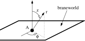
FIG. 1.: A schematic representation of a spatial slice through a cosmic string located at $A$. The coordinate $x$ along the cosmic string is suppressed. The coordinate $r$ represents the 3-dimensional distance from the cosmic string $A$, while the coordinate $z$ denotes the polar angle from the vertical axis. In the no-gravity limit, the braneworld is the horizontal plane, $z={\pi\over 2}$. The coordinate $\phi$ is the azimuthal coordinate. Note that everywhere except at the cosmic string, the unit vector in the direction of the $z$-coordinate extends perpendicularly from the brane into the bulk.

$$T_{tt}=-T_{xx}=N^{2}(r,z){T\ \delta(r)\over 2\pi A(r,z)B^{2}(r,z)\sin z}\ ,$$ (9)

where the parameter $T$ denotes the string tension and all other components of the energy-momentum tensor are zero. The Einstein equations dictated by the action Eqs. (5–6) are

$${1\over 2r_{0}}G_{AB}+{1\over B(r,z)}\delta\left(z-{\pi\alpha\over 2}\right)G^{(4)}_{AB}={1\over M_{P}^{2}}T_{AB}\ ,$$ (10)

where $G_{AB}$ is the five-dimensional Einstein tensor, $G^{(4)}_{AB}$ is the induced four-dimensional Einstein tensor on the brane, $T_{AB}$ is the energy-momentum on the brane Eq. (9), and we have defined a crossover scale

$$r_{0}={M_{P}^{2}\over 2M^{3}}\ .$$ (11)

This scale characterizes that distance over which metric fluctuations propagating on the brane dissipate into the bulk [10].

We assume a ${\cal Z}_{2}$–symmetric brane across $z={\pi\alpha\over 2}$. Under this circumstance, one may solve Eqs. (9–10) by solving $G_{AB}=0$ in the bulk, i.e., when $z<{\pi\alpha\over 2}$ and $r\neq 0$, such that the following brane boundary conditions apply at $z={\pi\alpha\over 2}$:

$$\left({N_{z}\over N}+{A_{z}\over A}+{B_{z}\over B}\right) = {r_{0}r\over A^{2}}\left[{N_{rr}\over N}-{N_{r}\over N}{A_{r}\over A}+{1\over r}\left({N_{r}\over N}-{A_{r}\over A}\right)\right]$$ (12)

$$\ \ \ \ \ \ \ \ \ \ \ \ \ \ \ \ \ \ \ \ \ \ \ \ \ \ -\ {\sqrt{1-\beta^{2}}\over\beta}\ +\ {r_{0}T/M_{P}^{2}\over 2\pi\beta}{1\over A}\delta(r)$$ (13)

$$\left(2{N_{z}\over N}+{B_{z}\over B}\right) = {r_{0}r\over A^{2}}\left[{N^{2}_{r}\over N^{2}}+{2\over r}{N_{r}\over N}\right]\ -\ {\sqrt{1-\beta^{2}}\over\beta}$$ (14)

$$\left(2{N_{z}\over N}+{A_{z}\over A}\right) = {r_{0}r\over A^{2}}\left[2{N_{rr}\over N}+{N^{2}_{r}\over N^{2}}-2{N_{r}\over N}{A_{r}\over A}\right]$$ (15)

where we have defined $\beta=\sin{\pi\alpha\over 2}$ and where the subscript represents partial differentiation with respect to the corresponding coordinate. Equations (14) follow from $G_{tt}$, $G_{rr}$ and $G_{\phi\phi}$, respectively, and are generated by the intrinsic curvature term induced by the action Eq. (6). We also impose boundary conditions to ensure continuity of the metric and its derivatives at $z=0$, and to fix a residual gauge degree of freedom by choosing $B(z={\pi\alpha\over 2})=r$.

We wish to find the full five-dimensional spacetime metric induced by a thin cosmic string situated within the braneworld. The problem defined by Eqs. (9–10) is dependent only on the scale $r_{0}$ and the dimensionless parameter ${T\over M_{P}^{2}}$. We are interested in the problem when $r_{0}\rightarrow\infty$ with all other parameters held fixed. Since $r_{0}$ represents the only scale in the problem, this statement implies we are interested in the system when $r\ll r_{0}$ with ${T\over M_{P}^{2}}$ fixed.

B The Einstein solution

Before we attempt to solve the full five-dimensional problem given by Eqs. (9–10) and Eq. (14), it is useful to review the cosmic string solution in simply four-dimensional Einstein gravity [15, 16]. For a cosmic string with energy momentum Eq. (9), the exact metric may be represented by the line element:

$$ds^{2}=dt^{2}-dx^{2}-\left(1-{T\over 2\pi M_{P}^{2}}\right)^{-2}dr^{2}-r^{2}d\phi^{2}\ .$$ (16)

This represents a flat space with a deficit angle ${T\over M_{P}^{2}}$. Thus, there is no Newtonian potential between a cosmic string and a static test particle. However, a test particle (massive or massless) suffers an azimuthal deflection of ${T\over M_{P}^{2}}$ when scattered around the cosmic string. With a different coordinate choice, the line element can be rewritten as

$$ds^{2}=dt^{2}-dx^{2}-(y^{2}+z^{2})^{-T/2\pi M_{P}^{2}}[dy^{2}+dz^{2}]\ .$$ (17)

Again, there is no Newtonian potential between a cosmic string and a static test particle. However, in this coordinate choice, the deflection of a moving test particle can be interpreted as resulting from a gravitomagnetic force generated by the cosmic string. We can ask whether this Einstein solution is recovered on the brane in the limit of the theory where the graviton linewidth vanishes. In this limit, gravity fluctuations originating on the brane are pinned on that surface indefinitely, implying that gravity should resemble a four-dimensional theory. However, the question remains whether the four-dimensional theory that results is Einstein gravity or some massless scalar-tensor theory instead.

C Linearized Five-Dimensional Einstein Equations

Let us examine the linearized form of the Einstein equations, Eqs. (10). We will see that the trick is to find an appropriate background (including boundary conditions) around which linearize. We take the following:

$$N(r,z) = 1+n(r,z)+\cdots$$ (18)

$$A(r,z) = 1+a(r,z)+\cdots$$ (19)

$$B(r,z) = r\left[1+b(r,z)+\cdots\ \right]\ ,$$ (20)

where it is assumed that the functions $\{n(r,z),a(r,z),b(r,z)\}\ll 1$ in the regimes of interest. Taking the $R_{tt}$-component of the Einstein equations, one find that the PDE for $n(r,z)$

$$r^{2}~{}n_{rr}+2rn_{r}+n_{zz}+{\cos{z}\over\sin{z}}n_{z}=0\ ,$$ (21)

may be decoupled from the others. Equation (21) is simply Laplace’s equation for the Newtonian potential, $n(r,z)$, reducing the determination of $g_{00}$ to a linear static potential problem (albeit, with unusual boundary conditions resulting from the presence of the brane). In order to determine $a(r,z)$ and $b(r,z)$, one can directly integrate the $G_{zz}$ and the $G_{zz}$ components of the Einstein equations, leaving

$$a(r,z) = -2n(r,z)+rf^{\prime}(r)\cos{z}+rg^{\prime}(r)+g(r)$$ (22)

$$b(r,z) = -2n(r,z)+f(r)\cos{z}+g(r)\ .$$ (23)

The functions $f(r)$ and $g(r)$ are to be determined by the brane boundary conditions, as well as the last remaining residual gauge. This technique for decomposing the linearized Einstein equations is the direct analog of that used in [17].

The brane boundary conditions Eqs. (14) in the linearized Einstein equations may be used to complete the determination of the metric components. The second two equations in Eqs. (14) both yield

$$\beta f(r)={\sqrt{1-\beta^{2}}\over\beta}-2r_{0}n_{r}(r)|_{\sin z=\beta}\ .$$ (24)

Combining this equation for $f(r)$ and fixing the gauge choice $b(r)|_{\sin{z}=\beta}=0$ gives

$$g(r)=2n(r)|_{\sin{z}=\beta}+{\sqrt{1-\beta^{2}}\over\beta}r_{0}n_{r}(r)|_{\sin{z}=\beta}-{1-\beta^{2}\over\beta^{2}}\ .$$ (25)

The remaining equation in Eqs. (14) is then used to set the brane condition for the Newtonian potential $n(r,z)$:

$$n_{z}|_{\sin z=\beta}=r_{0}\left[\left(r+{2r_{0}\over 3}{\sqrt{1-\beta^{2}}\over\beta}\right)n_{rr}+n_{r}\right]_{\sin z=\beta}\ +\ {r_{0}\over 3\beta^{2}}\delta(r)\left[\beta+\left({T\over 2\pi M_{P}^{2}}-1\right)\right]\ ,$$ (26)

where the coefficient of the $\delta$–function contribution to this condition comes from the matter source (as reflected in the first equation of Eqs. (14)) and from the step in $A(r,z)$ at $r=0$ necessary to maintain elementary flatness at the location of the string. Once one determines $n(r,z)$ using Eq. (21) and the boundary conditions Eq. (26) as well as $n_{z}(r)|_{z=0}=0$, then one can automatically read off $a(r,z)$ and $b(r,z)$ using Eqs. (22–25).

D The weak brane limit

Let us first identify the solution to Eqs. (9–10) and Eq. (14) in the weak field limit. Here, we presume that the metric deviates from a flat metric with a flat brane where the perturbations (of the bulk and the brane) are proportional to the strength of the source, ${T\over M_{P}^{2}}$, assuming this parameter is small. With the coordinate choice under consideration, one may keep the brane at $z={\pi\over 2}$ while still allowing for a brane extrinsic curvature of ${\cal O}({T\over M_{P}^{2}})$. We refer to this limit where the extrinsic curvature of the brane is perturbed around a $flat$ brane as the weak brane limit.

In this limit one may use the linearized equations established in the last subsection. The explicit solution to Eqs. (21) and (26) with $\beta=1$ is

$$n(r,z)=-{r_{0}\over 3}\left({T\over 2\pi M_{P}^{2}}\right)\int_{0}^{\infty}{dk\over 1+r_{0}k}~{}e^{-kr\cos z}J_{0}(kr\sin z)\ ,$$ (27)

where $J_{0}$ is the usual Bessel function of the first kind. One can then solve for $a(r,z)$ and $b(r,z)$ directly using Eqs. (22–25). One may also arrive at this result by applying the graviton propagator [10, 14] and approximating the gravitational potential through one-particle graviton exchange between the cosmic string source and a test particle in a Minkowski spacetime with a flat braneworld.

Two limits are of interest. The regime where $r\gg r_{0}$ represents the crossover from four-dimensional to five-dimensional behavior expected at the scale $r_{0}$. Graviton modes localized on the brane evaporate into the bulk over distances comparable to $r_{0}$. The presence of the brane becomes increasingly irrelevant as $r/r_{0}\rightarrow\infty$ and a cosmic string on the brane acts as a codimension-three object in the full bulk. Here the metric is asymptotically spherically symmetric (i.e., $z$-independent) while the Newtonian potential Eq. (27) becomes

$$n(r,z)=-\ {1\over 3}\left({T\over 2\pi M_{P}^{2}}\right){r_{0}\over r}\ +\ {\cal O}(r_{0}^{2}/r^{2})\ .$$ (28)

Using the metric Eq. (8), we find the metric on the brane is specified by the line element

$$ds^{2}=N^{2}(r)|_{\sin z=1}\ (dt^{2}-dx^{2})-A^{2}(r)|_{\sin z=1}\ dr^{2}-r^{2}d\phi^{2}\$$ (29)

with

$$N(r)|_{\sin z=1} = 1\ -\ {1\over 3}\left({T\over 2\pi M_{P}^{2}}\right){r_{0}\over r}\ +\ {\cal O}(r_{0}^{2}/r^{2})$$ (30)

$$A(r)|_{\sin z=1} = 1\ +\ {2\over 3}\left({T\over 2\pi M_{P}^{2}}\right){r_{0}\over r}\ +\ {\cal O}(r_{0}^{2}/r^{2})\ ,$$ (31)

recovering the Schwarzschild-like solution for a codimension-three object in five-dimensional spacetime with

$$r_{G}={r_{0}T\over 2\pi M_{P}^{2}}={T\over 4\pi M^{3}}$$ (32)

acting as the effective Schwarzschild radius.

In the complementary limit when $r\ll r_{0}$, we find that Eq. (27) becomes

$$n(r,z)={1\over 3}\left({T\over 2\pi M_{P}^{2}}\right)\ln\left[{r\over r_{0}}(1+\cos z)\right]\ +\ {\cal O}\left({T^{2}\over M_{P}^{4}}\right)\ .$$ (33)

Using the metric Eq. (29) on the brane, we find

$$N(r)|_{\sin z=1} = 1\ +\ {1\over 3}\left({T\over 2\pi M_{P}^{2}}\ln{r\over r_{0}}\right)\ +\ {\cal O}\left({T^{2}\over M_{P}^{4}}\right)$$ (34)

$$A(r)|_{\sin z=1} = 1\ +\ {2\over 3}{T\over 2\pi M_{P}^{2}}\ +\ {\cal O}\left({T^{2}\over M_{P}^{4}}\right)\ ,$$ (35)

which represents a conical space with deficit angle ${2\over 3}{T\over M_{P}^{2}}$. Recall that for pure four-dimensional Einstein gravity, this metric is $N(r)=1$ and $A(r)=(1-{T\over 2\pi M_{P}^{2}})^{-1}$, which again represents a flat conical space with deficit angle ${T\over M_{P}^{2}}$. Thus in the weak brane limit, we expect not only an extra light scalar field generating the Newtonian potential found in $N(r)$, but also a discrepancy in the deficit angle with respect to the Einstein solution. Moreover, since Eqs. (34–35) deviate from the four-dimensional Einstein solution, the brane boundary conditions Eq. (14) imply that the brane itself possess an extrinsic curvature whose magnitude is ${\cal O}({T\over M_{P}^{2}})$.

We can ask the domain of validity of the solution Eqs. (34–35). Examining the boundary conditions Eqs. (14) and the bulk Einstein equations $G_{AB}=0$ and comparing the size of terms neglected with respect to those included, we see that on the brane this solution is only valid when

$$r_{0}\sqrt{{T\over M_{P}^{2}}}\ll r\ll r_{0}\ .$$ (36)

The left-hand inequality of Eq. (36) is the one of interest. For values of $r$ violating this condition, nonlinear contributions to the Einstein tensor become important and the weak brane approximation breaks down. But this is precisely the regime we are interested in, since we wish to understand what happens when $r$ and ${T\over M_{P}^{2}}$ are fixed and $r_{0}\rightarrow\infty$. We need to find a solution in this regime.

E The $r/r_{0}\rightarrow 0$ limit

The weak brane approximation breaks down when the condition Eq. (36) does not apply. Outside this domain of validity, nonlinear contributions to the Einstein equations become important. However, by relaxing the condition that the braneworld be located at $\sin z=1$, a perturbative solution to the Einstein equations Eqs. (9–10) with the boundary conditions Eq. (14) can be found in the limit of interest when $r\ll r_{0}$ with ${T\over M_{P}^{2}}$ held fixed. We are still interested in the limit of a weak source, i.e., ${T\over M_{P}^{2}}\ll 1$, so that using the linearized equations establish in Sec. IIC is still applicable.

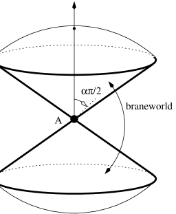
FIG. 2.: A spatial slice through the cosmic string located at $A$. As in Fig. 1 the coordinate $x$ along the cosmic string is suppressed. The solid angle wedge exterior to the cone is removed from the space, and the upper and lower branches of the cone are identified. This conical surface is the braneworld ($z={\pi\alpha\over 2}$ or $\sin z=\beta$). The bulk space now exhibits a deficit polar angle (cf. Fig. 1). Note that this deficit in polar angle translates into a conical deficit in the braneworld space.

Recall that the coordinate $z$ into the bulk acts as a polar angle, but where the space it parametrizes has a deficit polar angle. The bulk is characterized by that part of space where $\sin z<\beta$ (i.e., $0\leq z<{\pi\alpha\over 2}$ and $\pi(1-{\alpha\over 2})<z\leq\pi$) and the two surfaces where $\sin z=\beta$ are identified and together represent the braneworld. The identification of these two surfaces induces an extrinsic curvature contribution on the brane which is compensated by the braneworld’s intrinsic curvature. Note that the bulk is ${\cal Z}_{2}$–symmetric across the brane. The key difference between the analysis in this background and that in the previous subsection is the inclusion of nonperturbative extrinsic curvature in the background brane. Figure 2 depicts a spatial slice through the cosmic string.

One begins by solving the linearized Newtonian potential problem Eq. (21) with the boundary conditions Eq. (26) and $n_{z}(r)|_{z=0}=0$. Additional boundary conditions are necessary. In order to avoid the divergence of the fields $\{n(r,z),a(r,z),b(r,z)\}$ near the origin that leads to the importance of nonlinear contributions in the weak brane limit, we choose

$$n(z)|_{r=0}=0\ .$$ (37)

By specifying this boundary condition, one is required to constrain $\beta$ (with the brane located at $\sin z=\beta$) for consistency with the brane boundary condition, Eq. (26). In order to maintain consistency, the delta-function term must vanish, requiring

$$\beta=1-{T\over 2\pi M_{P}^{2}}\ .$$ (38)

One last boundary condition needs to be specified for large-$r$. We choose $n(r,z)$ to match asymptotically onto the form

$$n(z)|_{r=R}={1\over 3}\left({T\over 2\pi M_{P}^{2}}\right)\ln\left[{R\over r_{0}}(1+\cos z)\right]\ ,$$ (39)

for some $R$ such that $r_{0}\sqrt{T\over M_{P}^{2}}\ll R\ll r_{0}$. We choose this specific asymptotic form for reasons that will become clear in the next section. This boundary value problem for a static solution to Laplace’s equation Eq. (21) is well-posed, albeit in an unusual geometry and with unusual boundary conditions.

Unlike when $\sin z=1$, this solution to Laplace’s equation does not possess a simple closed form. However, one may articulate the dominant contributions to the Newtonian potential in several key limits. When $r\ll r_{0}\sqrt{{T\over M_{P}^{2}}}$

$$n(r,z)=\left[{1\over 2}\cos z\right]{r\over r_{0}}-\left[{1\over 2}P_{q}(\cos z)\right]\left({r\over r_{0}}\right)^{q}+\cdots\ ,$$ (40)

with $q=1+\sqrt{{T\over\pi M_{P}^{2}}}$ and $P_{q}(x)$ is the Legendre function of the first kind of order $q$. When $r\gg r_{0}\sqrt{{T\over M_{P}^{2}}}$,

$$n(r,z)={1\over 3}\left({T\over 2\pi M_{P}^{2}}\right)\ln\left[{3\over 2}{r\over r_{0}\sqrt{T\over 2\pi M_{P}^{2}}}(1+\cos z)\right]+\cdots\ .$$ (41)

Indeed, one can arrive at an explicit form for the leading contribution to the Newtonian potential on the brane itself:

$$n(r)={1\over 3}\left({T\over 2\pi M_{P}^{2}}\right)\ln\left[1~{}+~{}{3\over 2}{r\over r_{0}\sqrt{T\over 2\pi M_{P}^{2}}}\right]+\cdots\ ,$$ (42)

when $r\ll r_{0}$. One may ascertain $a(r,z)$ and $b(r,z)$ by directly using Eqs. (22–25). By comparing the full Einstein equations and brane boundary conditions, Eqs. (10–14), with the linearized equations, Eqs. (19–26), one can confirm that the Newtonian potential $n(r,z)$ is valid in the entire region $r\ll r_{0}$, while the expressions for $a(r,z)$ and $b(r,z)$ using Eqs. (22–25) are valid when $r\ll r_{0}\sqrt{{T\over M_{P}^{2}}}$ and when $r\gg r_{0}\sqrt{{T\over M_{P}^{2}}}$.

When $r\ll r_{0}\sqrt{T\over M_{P}^{2}}$, the metric on the brane is determined by the line element

$$ds^{2}=N^{2}(r)|_{\sin z=\beta}\ (dt^{2}-dx^{2})-A^{2}(r)|_{\sin z=\beta}\ dr^{2}-\beta^{2}r^{2}d\phi^{2}$$ (43)

with

$$N(r)|_{\sin z=\beta} = 1+{r\over 2r_{0}}\sqrt{T\over 2\pi M_{P}^{2}}\ +\ {\cal O}(r^{2}/r_{0}^{2})$$ (44)

$$A(r)|_{\sin z=\beta} = 1-{r\over 2r_{0}}\sqrt{T\over 2\pi M_{P}^{2}}\ +\ {\cal O}(r^{2}/r_{0}^{2})\ ,$$ (45)

where $\beta=1-\sqrt{T\over 2\pi M_{P}^{2}}$. The brane solution, Eqs. (44–45), is distinct from the weak brane solution, Eqs. (34–35). In particular, the extrinsic curvature of the brane in the first case is nonperturbative in the string tension, i.e., ${\cal O}(\sqrt{T\over M_{P}^{2}})$, whereas extrinsic curvature of the brane in the weak brane approximation is perturbative in the string tension, i.e., ${\cal O}({T\over M_{P}^{2}})$.

The deficit polar angle in the bulk is $\pi(1-\alpha)$ where again $\sin{\pi\alpha\over 2}=\beta$, while the deficit azimuthal angle in the brane itself is $2\pi(1-\beta)$. In the limit when $r_{0}\rightarrow\infty$, the graviton linewidth vanishes and we recover a flat conical space with a deficit angle $2\pi(1-\beta)={T\over M_{P}^{2}}$, the solution for a cosmic string in four-dimensional Einstein gravity Eq. (16). Consequently, the cosmic string solution Eqs. (44–45) does not suffer from a VDVZ discontinuity, supporting the results found for cosmological solutions [14] in this braneworld theory with a metastable brane graviton.

III Matching between Phases

We wish to address the matching of the Einstein phase, Eqs. (44–45) to the weak brane phase, Eqs. (34–35). These two solutions are in distinct coordinate systems. Nevertheless, when the cosmic string source strength ${T\over M_{P}^{2}}$ is small, there exists a region in $r$, namely $r_{0}\sqrt{T\over M_{P}^{2}}\ll r\ll r_{0}$, where both solutions are valid. In this section we show that there exists a coordinate transformation that takes the Einstein phase into the weak brane phase in this region, implying that these phases are simply different parts of the same solution.

In the region $r_{0}\sqrt{T\over M_{P}^{2}}\ll r\ll r_{0}$, the Einstein phase takes the form

$$n(r,z) = {1\over 3}\left({T\over 2\pi M_{P}^{2}}\right)\ln\left[{3\over 2}{r\over r_{0}\sqrt{T\over 2\pi M_{P}^{2}}}(1+\cos z)\right]+\cdots$$ (46)

$$a(r,z) = {2\over 3}{r_{0}\over r}\left({T\over 2\pi M_{P}^{2}}\right)\cos z+\cdots$$ (47)

$$b(r,z) = \left(\sqrt{T\over 2\pi M_{P}^{2}}-{2r_{0}\over 3r}{T\over 2\pi M_{P}^{2}}\right)\cos z+\cdots\ ,$$ (48)

where the brane is located at $\sin z=1-{T\over 2\pi M_{P}^{2}}$ (or $\cos z=\sqrt{T\over 2\pi M_{P}^{2}}$), and neglecting contributions of ${\cal O}({T\over M_{P}^{2}})$ but keeping leading order contributions, e.g., $\sim{T\over 2\pi M_{P}^{2}}{r_{0}\over r}$. The weak brane phase in the same region has the form

$$n(r,z) = {1\over 3}\left({T\over 2\pi M_{P}^{2}}\right)\ln\left[{r\over r_{0}}(1+\cos z)\right]+\cdots$$ (49)

$$a(r,z) = {2\over 3}{r_{0}\over r}\left({T\over 2\pi M_{P}^{2}}\right)\cos z+\cdots$$ (50)

$$b(r,z) = -{2\over 3}{r_{0}\over r}\left({T\over 2\pi M_{P}^{2}}\right)\cos z+\cdots\ ,$$ (51)

where the brane is located at $\cos z=0$, and where again contributions of ${\cal O}({T\over M_{P}^{2}})$ are neglected.

We have chosen a region, $r_{0}\sqrt{T\over M_{P}^{2}}\ll r\ll r_{0}$, such that the solution Eqs. (47) remains a valid solution to the linearized Einstein equations while undergoing the following linear coordinate transformation. Take a new polar variable, ${\cal Z}$, such that

$${\cal Z}=z+\sqrt{T\over 2\pi M_{P}^{2}}\sin z+{\cal O}\left({T\over 2\pi M_{P}^{2}}\right)\ .$$ (52)

Since

$$\sin{\cal Z}=\sin z\left[1+\sqrt{T\over 2\pi M_{P}^{2}}\cos z\right]+\cdots\ ,$$ (53)

the metric functions are still in the ansatz Eq. (8) with the new polar coordinate, ${\cal Z}$:

$$ds^{2}=N^{2}(r,{\cal Z})(dt^{2}-dx^{2})-A^{2}(r,{\cal Z})dr^{2}-B^{2}(r,{\cal Z})\left[d{\cal Z}^{2}+\sin^{2}{\cal Z}\ d\phi^{2}\right]\ .$$ (54)

Under this coordinate redefinition, when the brane is located at $\cos z=\sqrt{T\over 2\pi M_{P}^{2}}$, it is now located at

$$\cos{\cal Z}=\cos z-\sqrt{T\over 2\pi M_{P}^{2}}+\cdots=0\ +\ {\cal O}\left({T\over 2\pi M_{P}^{2}}\right)\ .$$ (55)

and with a time renormalization

$$\tau={t\over 1-{1\over 6}\left({T\over 2\pi M_{P}^{2}}\right)\ln{T\over 2\pi M_{P}^{2}}}$$ (56)

the Einstein phase takes the form

$$n(r,{\cal Z}) = {1\over 3}\left({T\over 2\pi M_{P}^{2}}\right)\ln\left[{r\over r_{0}}(1+\cos{\cal Z})\right]+\cdots$$ (57)

$$a(r,{\cal Z}) = {2\over 3}{r_{0}\over r}\left({T\over 2\pi M_{P}^{2}}\right)\cos{\cal Z}+\cdots$$ (58)

$$b(r,{\cal Z}) = -{2\over 3}{r_{0}\over r}\left({T\over 2\pi M_{P}^{2}}\right)\cos{\cal Z}+\cdots\ ,$$ (59)

with the brane located at $\cos{\cal Z}=0$, which is identical to Eq. (50) up to ${\cal O}({T\over M_{P}^{2}})$. Thus, one can match the Einstein phase solution with the weak brane solution using the coordinate transformation Eq. (52) and the time redefinition Eq. (56), implying that the Einstein phase in Sec. IIE and the weak brane phase in Sec. IID are parts of the same solution.

IV Discussion

In different parametric regimes, we find different qualitative behaviors for the brane metric around a cosmic string. For an observer at a distance $r\gg r_{0}$ from the cosmic string, where $r_{0}^{-1}$ characterizes the graviton’s effective linewidth, the cosmic string appears as a codimension-three object in the full bulk. The metric is Schwarzschild-like in this regime. When $r\ll r_{0}$, brane effects become important, and the cosmic string appears as a codimension-two object on the brane. When the source is weak (i.e., when the tension, $T$, of the string is much smaller than the square of the four-dimensional Planck scale, $M_{P}^{2}$), the Einstein solution with a deficit angle of ${T\over M_{P}^{2}}$ holds on the brane when $r\ll r_{0}\sqrt{{T\over M_{P}^{2}}}$. In the region on the brane when $r\gg r_{0}\sqrt{{T\over M_{P}^{2}}}$ (but still where $r\ll r_{0}$), the weak brane approximation prevails, the cosmic string exhibits a nonvanishing Newtonian potential and space suffers a deficit angle different from ${T\over M_{P}^{2}}$.

We identified a coordinate transformation connecting the weak brane phase, Eqs. (34–35), and the Einstein phase, Eqs. (44–45). Each phase is a linear solution which becomes strongly nonlinear outside of its domain of validity simply because the corresponding coordinate system in which each solution is linear differs from the other. The full nonlinear solution in this light is reminiscent of the ansatz introduced by Vainshtein [4] for the Schwarzschild solution in a massive gravity theory. Moreover, the presence of this weak brane phase at large distances from the cosmic string may have non-negligible consequences for the observational search for cosmic strings through gravitational lensing techniques [18]. For a GUT scale ($10^{16}$ GeV) cosmic string, the Einstein deficit angle for the string is $\sim 10^{-5}$. This implies that the light deflection by the string differs significantly from the predictions of general relativity at distances

$$r\sim r_{0}\sqrt{{M_{\rm GUT}^{2}\over M_{P}^{2}}}\sim 3\ {\rm Mpc}\ ,$$ (60)

where $r_{0}$ is taken to be today’s Hubble radius. Such a seemingly peculiar choice of $r_{0}$ is intriguing cosmologically [13, 19]. Detailed discussion on how such a correspondingly small fundamental Planck scale is possible without serious phenomenological obstacles may be found in [11, 12].

The solution presented here supports the Einstein solution near the cosmic string in the limit that $r_{0}\rightarrow\infty$. This observation suggests that the braneworld theory under consideration does not suffer from a van Dam–Veltman–Zakharov (VDVZ) discontinuity, corroborating the findings for cosmological solutions in the same theory [14]. Far from the source, the gravitational field is weak, and the geometry of the brane within the bulk is not substantially altered by the presence of the cosmic string. Propagation of the light scalar mode is permitted. However near the source, the gravitational fields induce a nonperturbative extrinsic curvature in the brane. That extrinsic curvature suppresses the coupling of the scalar mode to matter and only the tensor mode remains, thus Einstein gravity is recovered. As one takes $r_{0}\rightarrow\infty$, the region where the source induces a large brane extrinsic curvature grows with $r_{0}$, implying Einstein gravity is strictly recovered in this limit.

In this paper, we investigate the spacetime around a cosmic string on a brane in a five-dimensional braneworld theory that supports a metastable brane graviton. This system has the advantage of offering a semianalytic solution to the metric around a compact object, while still providing a clear example in which the VDVZ discontinuity manifests itself. The result may help shed light on the more difficult, more immediately relevant problem of a Schwarzschild-like spherical source in this braneworld theory. At the same time, the cosmic string solution is itself interesting and, should these objects exist in nature, would have testable phenomenological consequences.

- [1] Y. Iwasaki, Phys. Rev. D 2, 2255 (1970).
- [2] H. van Dam and M. J. G. Veltman, Nucl. Phys. B22, 397 (1970).
- [3] V. I. Zakharov, JETP Lett. 12, 312 (1970).
- [4] A. I. Vainshtein, Phys. Lett. B 39, 393 (1972).
- [5] D. G. Boulware and S. Deser, Phys. Rev. D 6, 3368 (1972).
- [6] I. I. Kogan, S. Mouslopoulos and A. Papazoglou, Phys. Lett. B 501, 140 (2001); I. I. Kogan, S. Mouslopoulos and A. Papazoglou, Phys. Lett. B 503, 173 (2001).
- [7] A. Karch and L. Randall, JHEP 0105, 008 (2001).
- [8] M. Porrati, Phys. Lett. B 498, 92 (2001).
- [9] A. Karch, E. Katz and L. Randall, arXiv:hep-th/0106261.
- [10] G. Dvali, G. Gabadadze and M. Porrati, Phys. Lett. B 485, 208 (2000).
- [11] G. R. Dvali, G. Gabadadze, M. Kolanovic and F. Nitti, Phys. Rev. D 64, 084004 (2001).
- [12] G. R. Dvali, G. Gabadadze, M. Kolanovic and F. Nitti, arXiv:hep-th/0106058.
- [13] C. Deffayet, Phys. Lett. B 502, 199 (2001).
- [14] C. Deffayet, G. R. Dvali, G. Gabadadze and A. I. Vainshtein, hep-th/0106001.
- [15] A. Vilenkin, Phys. Rev. D 23, 852 (1981).
- [16] R. Gregory, Phys. Rev. Lett. 59, 740 (1987).
- [17] A. Gruzinov, arXiv:astro-ph/0112246.
- [18] See the following and references therein: A. de Laix, L. M. Krauss and T. Vachaspati, Phys. Rev. Lett. 79, 1968 (1997); A. A. de Laix, Phys. Rev. D 56, 6193 (1997); J. P. Uzan and F. Bernardeau, Phys. Rev. D 63, 023004 (2001).
- [19] C. Deffayet, G. R. Dvali and G. Gabadadze, arXiv:astro-ph/0105068.