Ellipsoidal Black Hole – Black Tori Systems in 4D Gravity

Abstract

We construct new classes of exact solutions of the 4D vacuum Einstein equations which describe ellipsoidal black holes, black tori and combined black hole – black tori configurations. The solutions can be static or with anisotropic polarizations and running constants. They are defined by off–diagonal metric ansatz which may be diagonalized with respect to anholonomic moving frames. We examine physical properties of such anholonomic gravitational configurations and discuss why the anholonomy may remove the restriction that horizons must be with spherical topology.

I Introduction

Torus configurations of matter around black hole – neutron star objects are intensively investigated in modern astrophysics putten . One considers that such tori may radiate gravitational radiation powered by the spin energy of the black hole in the presence of non–axisymmetries; long gamma–ray bursts from rapidly spinning black hole–torus systems may represent hypernovae or black hole–neutron star coalescence. Thus the topic of constructing of exact vacuum and non–vacuum solutions with non–trivial topology in the framework of general relativity and extra dimension gravitational theories becomes of special importance and interest.

In the early 1990s, new solutions with non–sperical black hole horizons (black tori) were found lemos for different states of matter and for locally anti-de Sitter space times; for a recent review, see rev . Static ellipsoidal black hole, black tori, anisotropic wormhole and Taub NUT metrics and soltionic solutions of the vacuum and non–vacuum Einstein equations were constructed in Refs. v ; v2 . Non–trivial topology configurations (for instance, black rings) are intensively studied in extra dimension gravity emp ; vth ; vtor .

For four dimensional gravity (4D), it is considered that a number of classical theorems israel impose that a stationary, asymptotically flat, vacuum black hole solution is completely characterized by its mass and spin and event horizons of non–spherical topology are forbidden haw ; see cen for further discussion of this issue.

Nevertheless, there were constructed various classes of exact solutions in 4D and 5D gravity with non–trivial topology, anisotropies, solitonic configurations, running constants and warped factors, under certain conditions defining static configurations in 4D vacuum gravity. Such metrics were parametrized by off–diagonal ansazt (for coordinate frames) which can be effectively diagonalized with respect to certain anholonomic frames with mixtures of holonomic and anholonomic variables. The system of vacuum Einstein equations for such ansatz becomes exactly integrable and describe a new ”anholonomic nonlinear dynamics” of vacuum gravitational fields, which posses generic local anisotropy. The new classes of solutions may have locally isotropic limits, or can be associated to metric coefficients of some well known, for instance, black hole, cylindrical, or wormhole soutions.

There is one important question if such anholonomic (anisotropic) solutions can exist only in extra dimension gravity, with some specific effective reductions to lower dimensions, or the anholonomic transforms generate a new class of solutions even in general relativity theory which might be not restricted by the conditions of Israel–Carter–Robinson uniqueness and Hawking cosmic cenzorship theorems israel ; haw ?

In the present paper, we explore possible 4D ellipsoidal black hole – black torus systems which are defined by generic off–diagonal matrices and describe anholonomic vacuum gravitational configurations. We present a new class of exact solutions of 4D vacuum Einstein equations which can be associated to some exact solutions with ellipsoidal/toroidal horizons and signularities, and theirs superpositions, being of static configuration, or, in general, with nonlinear gravitational polarization and running constants. We also discuss implications of these anisotropic solutions to gravity theories and ponder possible ways to solve the problem with topologically non–trivial and deformed horizons.

The organization of this paper is as follows: In Sec. II, we consider ellipsoidal and torus deformations and anistoropic confromal transforms of the Schwarzschil metric. We introduce an off–diagonal ansatz which can be diagonalized by anholonomic transforms and compute the non–trivial components of the vacuum Einstein equations in Sec. III. In Sec. IV, we construct and analyze three types of exact static solutions with ellisoidal–torus horizons. Sec. V is devoted to generalization of such solutions for configurations with running constants and anisotropic polarizations. The conclusion and discussion are presented in Sec. VI.

II Ellipsoidal/Torus Deformations of Metrics

In this Section we analyze anholonomic transforms with ellipsoidal/torus deformations of the Scwarzschild solution to some off–diagonal metrics. We define the conditions when the  new ’deformed’ metrics are exact solutions of vacuum Einstein equations.

The Schwarzschild solution may be written in  isotropic spherical coordinates $(\rho,\theta,\varphi)$  ll

$$dS^{2} = -\rho_{g}^{2}\left(\frac{\widehat{\rho}+1}{\widehat{\rho}}\right)^{4}\left(d\widehat{\rho}^{2}+\widehat{\rho}^{2}d\theta^{2}+\widehat{\rho}^{2}\sin^{2}\theta d\varphi^{2}\right)$$

$$+\left(\frac{\widehat{\rho}-1}{\widehat{\rho}+1}\right)^{2}dt^{2},$$

where the isotropic radial coordinate $\rho$ is related with the usual radial coordinate $r$ via the relation $r=\rho\left(1+r_{g}/4\rho\right)^{2}$ for $r_{g}=2G_{[4]}m_{0}/c^{2}$ being the 4D gravitational radius of a point particle of mass $m_{0},$ $G_{[4]}=1/M_{P[4]}^{2}$ is the 4D Newton constant expressed via Plank mass $M_{P[4]}.$ In our further considerations, we put the light speed constant $c=1$ and re–scale the isotropic radial coordinate as $\widehat{\rho}=\rho/\rho_{g},$ with $\rho_{g}=r_{g}/4.$ The metric (II) is a vacuum static solution of 4D Einstein equations with spherical symmetry describing the gravitational field of a point particle of mass $m_{0}.$ It has a singularity for $r=0$ and a spherical horizon for $r=r_{g},$ or, in re–scaled isotropic coordinates, for $\widehat{\rho}=1.$ We emphasize that this solution is parametrized by a diagonal metric given with respect to holonomic coordinate frames.

We may introduce a new ’exponential’ radial coordinate $\varsigma=\ln\widehat{\rho}$ and write the Schwarzschild metric as

$$ds^{2} = -\rho_{g}^{2}b\left(\varsigma\right)\left(d\varsigma^{2}+d\theta^{2}+\sin^{2}\theta d\varphi^{2}\right)+a\left(\varsigma\right)dt^{2},$$ (2)

$$a\left(\varsigma\right) = \left(\frac{\exp\varsigma-1}{\exp\varsigma+1}\right)^{2},b\left(\varsigma\right)=\frac{\left(\exp\varsigma+1\right)^{4}}{(\exp\varsigma)^{2}}.$$ (3)

The condition of vanishing of coefficient $a\left(\varsigma\right),\exp\varsigma=1,$ defines the horizon 3D spherical hypersurface

$$\varsigma=\varsigma\left[\widehat{\rho}\left(\sqrt{x^{2}+y^{2}+z^{2}}\right)\right],$$

where $x,y$ and $z$ are usual Cartezian coordinates.

The 3D spherical line element

$$ds_{(3)}^{2}=d\varsigma^{2}+d\theta^{2}+\sin^{2}\theta d\varphi^{2},$$

may be written in arbitrary ellipsoidal, or toroidal, coordinates which transforms the spherical horizon equation into very sophysticate relations (with respect to new coordinates).

Our idea is to deform (renormalize) the coefficients (3), $a\left(\varsigma\right)\rightarrow A\left(\varsigma,\theta\right)$ and $b\left(\varsigma\right)\rightarrow B\left(\varsigma,\theta\right),$ as they would define a rotation ellipsoid and/or a toroidal horizon and symmetry (for simplicity, we shall consider the ellongated ellipsoid configuration; the flattened ellipsoids may be analyzed in a similar manner).  But such a diagonal metric with respect to ellipsoidal, or toroidal, local coordinate frame does not solve the vacuum Einstein equations. In order to generate a new vacuum solution we have to ”elongate” the differentials $d\varphi$ and $dt,$ i. e. to introduce some ”anholonomic transforms” (see details in vth ), like

$$d\varphi \rightarrow \delta\varphi+w_{\varsigma}\left(\varsigma,\theta,v\right)d\varsigma+w_{\theta}\left(\varsigma,\theta,v\right)d\theta,$$

$$dt \rightarrow \delta t+n_{\varsigma}\left(\varsigma,\theta,v\right)d\varsigma+n_{\theta}\left(\varsigma,\theta,v\right)d\theta,$$

for $v=\varphi$ (static configuration), or $v=t$ (running in time configuration) and find the conditions when $w$- and $n$–coefficients and the renormalized metric coefficients define off–diagonal metrics solving the Einstein equations and possessing some ellipsoidal and/or toroidal horizons and symmetries.

We shall define the 3D space ellipsoid – toroidal configuration in this manner: in the center of Cartezian coordinates we put an rotation ellipsoid ellongated along axis $z$ (its intersection by the $xy$–coordinat plane describes a circle of radius $\rho_{g}^{[e]}=\sqrt{x^{2}+y^{2}}\sim\rho_{g});$ the ellipsoid is surrounded by a torus with the same $z$ axis of symmetry, when $-z_{0}\leq z\leq z_{0},$ and the interections of the torus with the $xy$–coordinate plane describe two circles of radia $\rho_{g}^{[t]}-z_{0}=\sqrt{x^{2}+y^{2}}$ and $\rho_{g}^{[t]}+z_{0}=\sqrt{x^{2}+y^{2}};$ the parameters $\rho_{g}^{[e]},\rho_{g}^{[t]}$ and $z_{0}$ are chosen as to define not intersecting toroidal and ellipsoidal horizons, i. e. the conditions

$$\rho_{g}^{[t]}-z_{0}>\rho_{g}^{[e]}>0$$ (4)

are imposed.

II.1 Ellipsoidal Configurations

We shall consider the  rotation ellipsoid coordinates korn $(u,\lambda,\varphi)$ with $0\leq u<\infty,0\leq\lambda\leq\pi,0\leq\varphi\leq 2\pi,$ where $\sigma=\cosh u\geq 1,$ are related with the isotropic 3D Cartezian coordinates $\left(x,y,z\right)$ as

$$(x = \widetilde{\rho}\sinh u\sin\lambda\cos\varphi,$$ (5)

$$y = \widetilde{\rho}\sinh u\sin\lambda\sin\varphi,z=\widetilde{\rho}\cosh u\cos\lambda)$$

and define an elongated rotation ellipsoid hypersurface

$$\left(x^{2}+y^{2}\right)/(\sigma^{2}-1)+\tilde{z}^{2}/\sigma^{2}=\widetilde{\rho}^{2}.$$ (6)

with $\sigma=\cosh u.$ The 3D metric on a such hypersurface is

$$dS_{(3D)}^{2}=g_{uu}du^{2}+g_{\lambda\lambda}d\lambda^{2}+g_{\varphi\varphi}d\varphi^{2},$$

where

$$g_{uu} = g_{\lambda\lambda}=\widetilde{\rho}^{2}\left(\sinh^{2}u+\sin^{2}\lambda\right),$$

$$g_{\varphi\varphi} = \widetilde{\rho}^{2}\sinh^{2}u\sin^{2}\lambda.$$

We can relate the rotation ellipsoid coordinates
$\left(u,\lambda,\varphi\right)$ from (5) with the isotropic radial coordinates $\left(\widehat{\rho},\theta,\varphi\right)$, scaled by the constant $\rho_{g},$ from (II),   equivalently with coordinates $\left(\varsigma,\theta,\varphi\right)$ from (2), as

$$\widetilde{\rho}=1,\cosh u=\widehat{\rho}=\exp\varsigma$$

and deform the Schwarzschild metric by introducing ellipsoidal coordinates and a new horizon defined by the condition that vanishing of the metric coefficient before $dt^{2}$ describe an elongated rotation ellipsoid hypersurface (6),

$$ds_{E}^{2} = -\rho_{g}^{2}\left(\frac{\cosh u+1}{\cosh u}\right)^{4}(\sinh^{2}u+\sin^{2}\lambda)$$

$$\times[du^{2}+d\lambda^{2}+\frac{\sinh^{2}u~{}\sin^{2}\lambda}{\sinh^{2}u+\sin^{2}\lambda}d\varphi^{2}]$$

$$+\left(\frac{\cosh u-1}{\cosh u+1}\right)^{2}dt^{2}.$$

The ellipsoidally deformed metric (II.1) does not satisfy the vacuum Einstein equations, but at long distances from the horizon it transforms into the usual Schwarzchild solution (II).

We introduce two Classes (A and B) of 4D auxiliary pseudo–Riemannian metrics, also given in ellipsoid coordinates, being some conformal transforms of (II.1), like

$$ds_{E}^{2}=\Omega_{A(B)E}\left(u,\lambda\right)ds_{A(B)E}^{2}$$

which also are not supposed to be solutions of the Einstein equations:

Metric of Class A:

$$ds_{(AE)}^{2}=-du^{2}-d\lambda^{2}+a_{E}(u,\lambda)d\varphi^{2}+b_{E}(u,\lambda)dt^{2}],$$ (8)

where

$$a_{E}(u,\lambda) = -\frac{\sinh^{2}u~{}\sin^{2}\lambda}{\sinh^{2}u+\sin^{2}\lambda},$$ (9)

$$b_{E}(u,\lambda) = \frac{(\cosh u-1)^{2}\cosh^{4}u}{\rho_{g}^{2}(\cosh u+1)^{6}(\sinh^{2}u+\sin^{2}\lambda)},$$

which results in the metric (II.1) by multiplication on the conformal factor

$$\Omega_{AE}\left(u,\lambda\right)=\rho_{g}^{2}\frac{(\cosh u+1)^{4}}{\cosh^{4}u}(\sinh^{2}u+\sin^{2}\lambda).$$ (10)

Metric of Class B:

$$ds_{BE}^{2}=g_{E}(u,\lambda)\left(du^{2}+d\lambda^{2}\right)-d\varphi^{2}+f_{E}(u,\lambda)dt^{2},$$ (11)

where

$$g_{E}(u,\lambda) = -\frac{\sinh^{2}u+\sin^{2}\lambda}{\sinh^{2}u~{}\sin^{2}\lambda},$$

$$f_{E}(u,\lambda) = \frac{(\cosh u-1)^{2}\cosh^{4}u}{\rho_{g}^{2}(\cosh u+1)^{6}\sinh^{2}u\sin^{2}\lambda},$$ (12)

which results in the metric (II.1) by multiplication on the conformal factor

$$\Omega_{BE}\left(u,\lambda\right)=\rho_{g}^{2}\frac{(\cosh u+1)^{4}}{\cosh^{4}u}\sinh^{2}u\sin^{2}\lambda.$$

In Ref. vth we proved that there are anholonomic transforms of the metrics (II.1), (8) and (11) which results in exact ellipsoidal black hole solutions of the vacuum Einstein equations.

II.2 Toroidal Configurations

Fixing a scale parameter $\rho_{g}^{[t]}$ which satisfies the conditions (4) we define the  toroidal coordinates $(\sigma,\tau,\varphi)$ (we emphasize that in in this paper we use different letters for ellipsoidal and toroidal coordinates introduced in Ref. korn ). These coordinates run the values $-\pi\leq\sigma<\pi,0\leq\tau\leq\infty,0\leq\varphi<2\pi.$ They are related with the isotropic 3D Cartezian coordinates via transforms

$$\tilde{x} = \frac{\widetilde{\rho}\sinh\tau}{\cosh\tau-\cos\sigma}\cos\varphi,$$ (13)

$$\tilde{y} = \frac{\widetilde{\rho}\sinh\tau}{\cosh\tau-\cos\sigma}\sin\varphi,\tilde{z}=\frac{\widetilde{\rho}\sinh\sigma}{\cosh\tau-\cos\sigma}$$

and define a toroidal hypersurface

$$\left(\sqrt{\tilde{x}^{2}+\tilde{y}^{2}}-\widetilde{\rho}\frac{\cosh\tau}{\sinh\tau}\right)^{2}+\tilde{z}^{2}=\frac{\widetilde{\rho}^{2}}{\sinh^{2}\tau}.$$

The 3D metric on a such toroidal hypersurface is

$$ds_{(3D)}^{2}=g_{\sigma\sigma}d\sigma^{2}+g_{\tau\tau}d\tau^{2}+g_{\varphi\varphi}d\varphi^{2},$$

where

$$g_{\sigma\sigma} = g_{\tau\tau}=\frac{\widetilde{\rho}^{2}}{\left(\cosh\tau-\cos\sigma\right)^{2}},$$

$$g_{\varphi\varphi} = \frac{\widetilde{\rho}^{2}\sinh^{2}\tau}{\left(\cosh\tau-\cos\sigma\right)^{2}}.$$

We can relate the toroidal coordinates $\left(\sigma,\tau,\varphi\right)$ from (13) with the isotropic radial coordinates $\left(\widehat{\rho}^{[t]},\theta,\varphi\right)$, scaled by the constant $\rho_{g}^{[t]},$ as

$$\widetilde{\rho}=1,\sinh^{-1}\tau=\widehat{\rho}^{[t]}$$

and transform the Schwarzschild solution into a new metric with toroidal coordinates  by changing the 3D radial line element into the toroidal one and stating the $tt$–coefficient of the metric to have a toroidal horizon. The resulting metric is

$$ds_{T}^{2} = -\left(\rho_{g}^{[t]}\right)^{2}\frac{\left(\sinh\tau+1\right)^{4}}{\left(\cosh\tau-\cos\sigma\right)^{2}}\times$$

$$\left(d\sigma^{2}+d\tau^{2}+\sinh^{2}\tau d\varphi^{2}\right)+\left(\frac{\sinh\tau-1}{\sinh\tau+1}\right)^{2}dt^{2},$$

Such a deformed Schwarzchild like toroidal metric is not an exact solution of the vacuum Einstein equations, but at long radial distances it transforms into the usual Schwarzchild solution with effective horizon $\rho_{g}^{[t]}$ with the 3D line element parametrized by toroidal coordinates.

We introduce two Classes (A and B) of 4D auxiliary pseudo-Riemannian metrics, also given in toroidal coordinates, being some conformal transforms of (II.2), like

$$ds_{T}^{2}=\Omega_{A(B)T}\left(\sigma,\tau\right)ds_{A(B)T}^{2}$$

but which are not supposed to be solutions of the Einstein equations:

Metric of Class A:

$$ds_{AT}^{2}=-d\sigma^{2}-d\tau^{2}+a_{T}(\tau)d\varphi^{2}+b_{T}(\sigma,\tau)dt^{2},$$ (15)

where

$$a_{T}(\tau) = -\sinh^{2}\tau,$$

$$b_{T}(\sigma,\tau) = \frac{\left(\sinh\tau-1\right)^{2}\left(\cosh\tau-\cos\sigma\right)^{2}}{\rho_{g}^{[t]2}\left(\sinh\tau+1\right)^{6}},$$ (16)

which results in the metric (II.2) by multiplication on the conformal factor

$$\Omega_{AT}\left(\sigma,\tau\right)=\rho_{g}^{[t]2}\frac{\left(\sinh\tau+1\right)^{4}}{\left(\cosh\tau-\cos\sigma\right)^{2}}.$$ (17)

Metric of Class B:

$$ds_{BT}^{2}=g_{T}(\tau)\left(d\sigma^{2}+d\tau^{2}\right)-d\varphi^{2}+f_{T}(\sigma,\tau)dt^{2},$$ (18)

where

$$g_{T}(\tau) = -\sinh^{-2}\tau,$$

$$f_{T}(\sigma,\tau) = \rho_{g}^{[t]2}\left(\frac{\sinh^{2}\tau-1}{\cosh\tau-\cos\sigma}\right)^{2},$$

which results in the metric (II.2) by multiplication on the conformal factor

$$\Omega_{BT}\left(\sigma,\tau\right)=\left(\rho_{g}^{[t]}\right)^{-2}\frac{\left(\cosh\tau-\cos\sigma\right)^{2}}{\left(\sinh\tau+1\right)^{2}}.$$ (19)

In Ref. vtor we used the metrics (II.2), (15) and (18) in order to generate exact solutions of the Einstein equations with toroidal horizons and anisotropic polarizations and running constants by performing corresponding anholonomic transforms.

III The Metric Ansatz and Vacuum Einstein Equations

Let us denote the local system of coordinates as $u^{\alpha}=\left(x^{i},y^{a}\right),$ where $\ x^{1}=u$ and $x^{2}=\lambda$ for ellipsoidal coordinates ($x^{1}=\sigma$ and $x^{2}=\tau$ for toroidal coordinates) and $y^{3}=v=\varphi$ and $y^{4}=t$ for the so–called $\varphi$–anisotropic configurations ($y^{4}=v=t$ and $y^{5}=\varphi$ for the so–called $t$–anisotropic configurations). Our spacetime is modeled as a 4D pseudo–Riemannian space of signature $\left(-,-,-,+\right)$ (or $\left(-,-,+,-\right)),$ which in general may be enabled with an anholonomic frame structure (tetrads, or vierbiend) $e_{\alpha}=A_{\alpha}^{\beta}\left(u^{\gamma}\right)\partial/\partial u^{\beta}$ subjected to some anholonomy  relations

$$e_{\alpha}e_{\beta}-e_{\beta}e_{\alpha}=W_{\alpha\beta}^{\gamma}\left(u^{\varepsilon}\right)e_{\gamma},$$ (20)

where $W_{\alpha\beta}^{\gamma}\left(u^{\varepsilon}\right)$ are called the coefficients of anholonomy.

The anholonomically and conformally transformed 4D line element is

$$ds^{2}=\Omega^{2}(x^{i},v)\hat{{g}}_{\alpha\beta}\left(x^{i},v\right)du^{\alpha}du^{\beta},$$ (21)

were the coefficients $\hat{{g}}_{\alpha\beta}$ are parametrized by the ansatz

$$\left[\begin{array}[]{cccc}g_{1}+\zeta_{1}^{\ 2}h_{3}+n_{3}^{\ 2}h_{4}&\zeta_{1}\zeta_{2}h_{3}+n_{1}n_{2}h_{4}&\zeta_{1}h_{3}&n_{1}h_{4}\\ \zeta_{1}\zeta_{2}h_{3}+n_{1}n_{2}h_{4}&g_{2}+\zeta_{2}^{\ 2}h_{3}+n_{3}^{\ 2}h_{4}&+\zeta_{2}h_{3}&n_{2}h_{4}\\ \zeta_{1}h_{3}&\zeta_{2}h_{3}&h_{3}&0\\ n_{1}h_{4}&n_{2}h_{4}&0&h_{4}\end{array}\right],$$ (22)

with $g_{i}=g_{i}\left(x^{i}\right),h_{a}=h_{ai}\left(x^{k},v\right),n_{i}=n_{i}\left(x^{k},v\right),$ $\zeta_{i}=\zeta_{i}\left(x^{k},v\right)$    and $\Omega=\Omega\left(x^{k},v\right)$ being some functions of necessary smoothly class or even sigular in some points and finite regions. So, the $g_{i}$–components of our ansatz depend only on ”holonomic” variables $x^{i}$ and the rest of coefficients may also depend on ”anisotropic” (anholonomic) variable $y^{3}=v;$ our ansatz does not depend on the second anisotropic variable $y^{4}.$

We may diagonalize the line element

$$\delta s^{2}=\Omega^{2}[g_{1}(dx^{1})^{2}+g_{2}(dx^{2})^{2}+h_{3}(\delta v)^{2}+h_{4}(\delta y^{4})^{2}],$$ (23)

with respect to the anholonomic co–frame
$\delta^{\alpha}=\left(dx^{i},\delta v,\delta y^{4}\right),$ where

$$\delta v=dv+\zeta_{i}dx^{i}\mbox{ and }\delta y^{4}=dy^{4}+n_{i}dx^{i},$$ (24)

which is dual to the frame $\delta_{\alpha}=\left(\delta_{i},\partial_{4},\partial_{5}\right),$ where

$$\delta_{i}=\partial_{i}+\zeta_{i}\partial_{3}+n_{i}\partial_{4}.$$ (25)

The tetrads $\delta_{\alpha}$ and $\delta^{\alpha}$ are anholonomic because, in general, they satisfy some non–trivial anholonomy relations (20). The anholonomy is induced by the coefficients $\zeta_{i}$ and $n_{i}$ which ”elongate” partial derivatives and differentials if we are working with respect to anholonomic frames. This result in a more sophisticate differential and integral calculus (a usual situation in ’tetradic’ and ’spinor’ gravity), but simplifies substantially tensor computations, because we are dealing with diagonalized metrics.

The vacuum Einstein equations for the (22) (equivalently, for (23)), $R_{\alpha}^{\beta}=0,$ computed with respect to anholonomic frames (24) and (25), transforms into a system of partial differential equations v ; vth ; vtor :

$$R_{1}^{1}=R_{2}^{2}=-\frac{1}{2g_{1}g_{2}}[g_{2}^{\bullet\bullet}-\frac{g_{1}^{\bullet}g_{2}^{\bullet}}{2g_{1}}-\frac{(g_{2}^{\bullet})^{2}}{2g_{2}}$$

$$+g_{1}^{{}^{\prime\prime}}-\frac{g_{1}^{{}^{\prime}}g_{2}^{{}^{\prime}}}{2g_{2}}-\frac{(g_{1}^{{}^{\prime}})^{2}}{2g_{1}}] = 0,$$ (26)

$$R_{3}^{3}=R_{4}^{4}=\frac{-1}{2h_{3}h_{4}}\left[h_{4}^{\ast\ast}-h_{4}^{\ast}\left(\ln\sqrt{|h_{3}h_{4}|}\right)^{\ast}\right] = 0,$$ (27)

$$R_{4i}=-\frac{h_{4}}{2h_{3}}\left[n_{i}^{\ast\ast}+\gamma n_{i}^{\ast}\right] = 0,$$ (28)

where

$$\gamma=3h_{4}^{\ast}/2h_{4}-h_{3}^{\ast}/h_{3},$$ (29)

and the partial derivatives are abreviated like $g_{1}^{\bullet}=\partial g_{1}/\partial x^{1},g_{1}^{{}^{\prime}}=\partial g_{1}/\partial x^{2}$ and $h_{3}^{\ast}=\partial h_{3}/\partial v.$ The coefficients $\zeta_{{i}}$ are found as to consider non–trivial conformal factors $\Omega:$ we compensate by $\zeta_{{i}}$ possible conformal deformations of the Ricci tensors, computed with respect to anholonomic frames. The conformal invariance of such anholonomic transforms holds if

$$\Omega^{q_{1}/q_{2}}=h_{3}~{}(q_{1}\mbox{ and }q_{2}\mbox{ are integers}),$$ (30)

and there are satisfied the equations

$$\partial_{i}\Omega-\zeta_{{i}}\Omega^{\ast}=0.$$ (31)

The system of equations (26)–(28) and (31) can be integrated in general form vth . Physical solutions are defined from some additional boundary conditions, imposed types of symmetries, nonlinearities and singular behaviour and compatibility in locally anisotropic limits with some well known exact solutions.

In this paper we give some examples of ellipsoidal and toroidal solutions and investigate some classes of metrics for combined ellipsoidal black hole – black tori configurations.

IV Static Black Hole – Black Torus Metrics

We analyzed in detail the method of anholonomic frames and constructed 4D and 5D ellipsoidal black hole and black tori solutions in Refs. v ; vth ; vtor . In this Section we give same new examples of metrics describing  one static 4D black hole  or one static 4D black torus configurations. Then we extend the constructions for metrics describing combined variants of black hole – black torus solutions. We shall analyze solutions with trivial and non–trivial conformal factors.

In this section the 4D local coordinates are written as $\left(x^{1},x^{2},y^{3}=v=\varphi,y^{4}=t\right),$ where we take $x^{i}=(u,\lambda)$ for ellipsoidal configurations and $x^{i}=(\sigma,\tau)$ for toroidal configurations. Here we note that, we can introduce a ”general” 2D space ellipsoidal coordinate system, $u=u(\sigma,\tau)$ and $\lambda=\tau,$ for both ellipsoidal and toroidal configurations if, for instance, we identify the ellipsoidal coordinate $\lambda$ with the toroidal $\tau,$ and relate $u$ with $\sigma$ and $\tau$ as

$$\sinh u=\frac{1}{\cosh\tau-\cos\sigma}.$$

In the vicinity of $\tau=0$ we can aproximate $\cosh\tau\approx 1$ and to write $u=u\left(\sigma\right)$and $\lambda=\tau.$ For $\tau\gg 1$ we have

$$\sinh u\approx\frac{1}{\cosh\tau}\left(1+\frac{1}{\cos\sigma}\right).$$

In general, we consider that the ”holonomic” coordinates are some functions $x^{i}=x^{i}\left(\sigma,\tau\right)=\widetilde{x}^{i}\left(u,\lambda\right)$ for which the 2D line element can be written in conformal metric form,

$$ds_{[2]}^{2}=-\mu^{2}\left(x^{i}\right)\left[\left(dx^{1}\right)^{2}+\left(dx^{2}\right)^{2}\right].$$

For simlicity, we consider 4D coordinate parametrizations when the angular coordinate $\varphi$ and the time like coordinate $t$ are not affected by any transforms of $x$-coordinates.

IV.1 Static anisotropic black hole/torus solutions

IV.1.1 An example of ellipsoidal black hole configuration

The symplest way to generate a static but anisotropic ellipsoidal black hole solution with an anholonomically diagonalized metric (23) is  to take a metric of type (8), to ”elongate” its differentials,

$$d\varphi \rightarrow \delta\varphi=d\varphi+\zeta_{i}\left(x^{k},\varphi\right)dx^{i},$$

$$dt \rightarrow \delta t=dt+n_{i}\left(x^{k},\varphi\right)dx^{i},$$

than to multiply on a conformal factor

$$\Omega^{2}\left(x^{k},\varphi\right)=\omega^{2}\left(x^{k},\varphi\right)\Omega_{AE}^{2}(x^{k}),$$

the factor $\omega^{2}\left(x^{k},\varphi\right)$ is obtained by rescaling the consant $\rho_{g}$ from (10),

$$\rho_{g}\rightarrow\overline{\rho}_{g}=\omega\left(x^{k},\varphi\right)\rho_{g},$$ (32)

in the simplest case we can consider only ”angular” on $\varphi$ anisotropies. Then we ’renormalize’ (by introducing $x^{i}$ coordinates) the $g_{1},g_{2}$ and $h_{3}$ coefficients,

$$g_{1,2} = -1\rightarrow-\mu^{2}\left(x^{i}\right),$$ (33)

$$h_{3} = h_{3[0]}=a_{E}(u,\lambda)\rightarrow h_{3}=-\Omega^{-2}\left(x^{k},\varphi\right),$$ (34)

we fix a relation of type (30), and take $h_{4}=$ $h_{4[0]}=b_{E}(x^{i}).$ The anholonomically transformed metric is parametrized in the form

$$\delta s^{2} = \Omega^{2}\{-\mu^{2}\left(x^{i}\right)\left[(dx^{1})^{2}+(dx^{2})^{2}\right]$$

$$-\Omega^{-2}\left(x^{k},\varphi\right)(\delta v)^{2}+b_{E}(x^{i})(\delta y^{4})^{2}\},$$

where $\mu,\zeta_{i}$ and $n_{i}$ are to be defined respectively from the equations (26), (31) and (28). We note that the equation (27) is already solved because in our case $h_{4}^{\ast}=0.$

The equation (26), with partial derivations on coordinates $x^{i}$ and parametrizations (33) has the general solution

$$\mu^{2}=\mu_{[0]}^{2}\exp\left[c_{[1]}x^{1}\left(u,\lambda\right)+c_{[2]}x^{2}\left(u,\lambda\right)\right],$$ (36)

where $\mu_{[0]},c_{[1]}$ and $c_{[2]}$ are some constants which should be defined from boundary conditions and by fixing a corresponding 2D system of coordinates; we pointed that we may redefine the factor (36) in ’pure’ ellipsoidal coordinates $\left(u,\lambda\right).$

The general solution of (31) for renormalization (32) and parametrization (34) is

$$\zeta_{i}\left(x^{k},\varphi\right) = \left(\omega^{\ast}\right)^{-1}\partial_{i}\omega+\partial_{i}\ln|\Omega_{AE}|/\left(\ln|\omega|\right)^{\ast},$$

$$= \partial_{i}\ln|\Omega_{AE}|/\left(\ln|\omega|\right)^{\ast}\mbox{ for }\omega=\omega\left(\varphi\right).$$

For a given $h_{3}$ with $h_{4}^{\ast}=0,$ we can compute the coefficient $\gamma$ from (29). After two integrations on $\varphi$ in (28) we find

$$n_{i}\left(x^{k},\varphi\right)=n_{i[0]}\left(x^{k}\right)+n_{i[1]}\left(x^{k}\right)\int\omega^{-2}d\varphi.$$ (38)

The set of functions (36), (IV.1.1) and (38) for any given $\Omega_{AE}\left(x^{i}\right)$ and $\omega\left(x^{k},\varphi\right)$ defines an exact static solution of the vacuum Einstein equations parametrized by an off–diagonal metric of type (IV.1.1). This solution have an ellipsoidal horizon defined by the condition of vanishing of the coefficient $h_{4[0]}=b_{E}(x^{i}),$ see the coefficients for the auxiliarry metric (8) and an anisotropic effective constant (32). This is a general solution depending on arbitrary functions $\omega\left(x^{k},\varphi\right)$ and $n_{i[0,1]}\left(x^{k}\right)$ and constants $\mu_{[0]},c_{[1]}$ and $c_{[2]}$ which have to be stated from some additional physical arguments.

For instance, if we wont to impose the condition that our solution, far away from the ellipsoidal horizon, transform into the Scwarzshild solution with an effective anisotropic ”mass”, or a renromalized gravitational Newton constant, we may put $\mu_{[0]}=1$ and fix the $x^{i}$–coordinates and constants $c_{[1,2]}$ as to obtain the linear interval

$$ds_{[2]}^{2}=-\left[du^{2}+d\lambda^{2}\right].$$

The coefficients $n_{i[0,1]}\left(x^{k}\right)$ and $\omega\left(x^{k},\varphi\right)$ may be taken as at long distances from the horizon one holds the limits $n_{i[0,1]}\left(x^{k}\right)\rightarrow 0$ and $\zeta_{i}\left(x^{k},\varphi\right)\rightarrow 0$ for $\omega\left(x^{k},\varphi\right)\rightarrow 0.$ In this case, at asymptotics, our solution will transform into a Schwarzshild like solution with ”renormalized” parameter $\overline{\rho}_{g}\rightarrow const.$

Nevertheless, we consider that it is not obligatory to select only such type of ellipsoidal solutions (with imposed asymptotic spherical symmetry) parametrized by metrics of class (IV.1.1). The system of vacuum gravitational equations (26)–(31) for the ansatz (IV.1.1) defines a nonlinear static configuration (an alternative vacuum Einstein configuration with ellipsoidal horizon) which, in general, is not equivalent to the Schwarschild vacuum. This points to some specific properties of the gravitational vacuum which follow from the nonlinear character of the Einstein equations. In quantum field theory the nonlinear effects may result in unitary non–equivalent vacua; in classical gravitational theories we could obtain a similar behaviour if we are dealing with off–diagonal metrics and anholonomic frames.

The constructed new static vacuum solution (IV.1.1) for a 4D ellipsoidal black hole is stated by the coefficients

$$g_{1,2} = -1,\mu=1,\overline{\rho}_{g}=\omega\left(x^{k},\varphi\right)\rho_{g},\Omega^{2}=\omega^{2}\Omega_{AE}^{2},$$

$$h_{3} = -\Omega^{-2}\left(x^{k},\varphi\right),h_{4}=b_{E}(x^{i}),(\mbox{ see (\ref{auxm1}),(\ref{auxm1c})}),$$

$$\zeta_{i} = \left(\omega^{\ast}\right)^{-1}\partial_{i}\omega+\partial_{i}\ln|\Omega_{AE}|/\left(\ln|\omega|\right)^{\ast},$$

$$n_{i} = n_{i[0]}\left(x^{k}\right)+n_{i[1]}\left(x^{k}\right)\int\omega^{-2}d\varphi.$$ (39)

These data define an ellipsoidal configuration, see Fig. 1.

Finally, we remark that we have generated a vacuum ellipsoidal gravitational configuration starting from the metric (8), i. e. we constructed an ellipsoidal $\varphi$–solution of Class A (see details on classification in vth ). In a similar manner we can define anholonomic deformations of the metric (11) and renormalization of conformal factor $\Omega_{BE}\left(u,\lambda\right)$ in order to construct an ellipsoidal $\varphi$–solution of Class B. We omit such considerations in this paper but present, in the next subsection, an example of toroidal $\varphi$–solution of Class B.

IV.1.2 An example of toroidal black hole configuration

We start with the metric (18), ”elongate” its differentials $d\varphi\rightarrow\delta\varphi$ and $dt\rightarrow\delta t$ and than multiply on a conformal factor

$$\Omega^{2}\left(x^{k},\varphi\right)=\varpi^{2}\left(x^{k},\varphi\right)\Omega_{BT}^{2}(x^{k})g_{T}\left(\tau\right),$$

see (19) which is connected with the renormalization of constant $\rho_{g}^{[t]},$

$$\rho_{g}^{[t]}\rightarrow\overline{\rho}_{g}^{[t]}=\varpi\left(x^{k},\varphi\right)\rho_{g}^{[t]}.$$ (40)

For toroidal configurations it is naturally to use 2D toroidal holonomic coordinates $x^{i}=(\sigma,\tau).$

The anholonomically transformed metric is parametrized in the form

$$\delta s^{2} = \Omega^{2}\{-\left[d\sigma^{2}+d\tau^{2}\right]-\eta_{3}\left(\sigma,\tau,\varphi\right)g_{T}^{-1}\left(\tau\right)\delta\varphi^{2}$$ (41)

$$+f_{T}(\sigma,\tau)g_{T}^{-1}\left(\tau\right)\delta t^{2}\}.$$

We state the coefficients

$$h_{3}=-\eta_{3}\left(\sigma,\tau,\varphi\right)g_{T}^{-1}\left(\tau\right)\mbox{ and }h_{4}=f_{T}(\sigma,\tau)g_{T}^{-1}\left(\tau\right),$$

where the polarization

$$\eta_{3}\left(\sigma,\tau,\varphi\right)=\varpi^{-2}\left(\sigma,\tau,\varphi\right)\Omega_{BT}^{-2}(\sigma,\tau)$$

is found from the condition (30) as $h_{3}=-\Omega^{-2}.$ The equation (27) is solved by arbitrary couples $h_{3}\left(\sigma,\tau,\varphi\right)$   and $h_{4}(\sigma,\tau)$ when $h_{4}^{\ast}=0.$ The procedure of definition of $\zeta_{i}\left(\sigma,\tau,\varphi\right)$ and $n_{i}\left(\sigma,\tau,\varphi\right)$ is similar to that from the previous subsection. We present the final results as the data

$$g_{1,2} = -1,\overline{\rho}_{g}=\varpi\left(\sigma,\tau,\varphi\right)\rho_{g},\Omega^{2}=\varpi^{2}\Omega_{BT}^{2}g_{T}\left(\tau\right),$$

$$h_{3} = -\eta_{3}\left(\sigma,\tau,\varphi\right)g_{T}^{-1}\left(\tau\right),h_{4}=f_{T}(\sigma,\tau)g_{T}^{-1}\left(\tau\right),$$

$$\eta_{3} = \varpi^{-2}\left(\sigma,\tau,\varphi\right)\Omega_{BT}^{-2}(\sigma,\tau),(\mbox{ see (\ref{auxm2t}), (\ref{auxm2tbc})}),$$

$$\zeta_{i} = \left(\varpi^{\ast}\right)^{-1}\partial_{i}\varpi+\partial_{i}\ln|\Omega_{BT}\sqrt{g_{T}}|/\left(\ln|\varpi|\right)^{\ast},$$ (42)

$$n_{i} = n_{i[0]}\left(\sigma,\tau\right)+n_{i[1]}\left(\sigma,\tau\right)\int\varpi^{-2}d\varphi$$

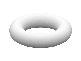
Figure 2: Toroidal Configuration

for the ansatz (41) which defines an exact static solution of the vacuum Einstein equations with toroidal symmetry, of Class B, with anisotropic dependence on coordinate $\varphi,$ see the torus configuration from Fig. 2. The off–diagonal solution is non–trivial for anisotropic linear distributions of mass on the circle contained in the torus ring, or alternatively, if there is a renormalized gravitational constant with anisotropic dependence on angle $\varphi.$ This class of solutions have a toroidal horizon defined by the condition of vanishing of the coefficient $h_{4}$ which holds if $f_{T}(\sigma,\tau)=0.$ The functions $\varpi\left(\sigma,\tau,\varphi\right)$ and $n_{i[0,1]}\left(\sigma,\tau\right)$ may be stated in a form that at long distancies from the toroidal horizon the (41) with data (42) will have asymptotics like the Scwarzschild metric. We can also consider alternative toroidal vacuum configurations. We note that instead of relations like $h_{3}=-\Omega^{-2}$ we can use every type $h_{3}\sim\Omega^{p/q},$ like is stated by (30); it depends on what type of nonlinear configuration and asymptotic limits we wont to obtain.

We remark also that in a symilar manner we can generate toroidal configurations of Class A, starting from the auxiliary metric (15). In the next subsection we elucidate this possibility by interfering it with a Class B ellipsoidal configuration.

IV.2 Static Ellipsoidal Black Hole – Black Torus solutions

There are different possibilities to combine static ellipsoidal black hole and black torus solutions as they will give configurations with two horizons. In this subsection we analyze two such variants. We consider a 2D system of holonomic coordinates $x^{i},$ which may be used both on the ’ellipsoidal’ and ’toroidal’ sectors via transforms like $u=u(x^{i}),\lambda=\tau\left(x^{i}\right)$ and $\sigma=\sigma\left(x^{i}\right).$

IV.2.1 Ellipsoidal–torus black configurations of Class BA

We construct a 4D vacuum metric with posses two type of horizons, ellipsoidal and toroidal one, having both type characteristics like a metic of Class B for ellipsoidal configurations and a metric of Class A for toroidal configurations (we conventionally call this ellipsoidal torus metric to be of Class BA).  The ansatz is taken

$$\delta s^{2} = \Omega^{2}\{-\mu^{2}\left(x^{i}\right)\left[(dx^{1})^{2}+(dx^{2})^{2}\right]$$

$$-\eta_{3}\left(x^{k},\varphi\right)a_{T}\left(x^{i}\right)\delta\varphi^{2}+\frac{b_{T}(x^{i})f_{E}(x^{i})}{g_{E}(x^{i})}\delta t^{2}\},$$

with

$$\Omega^{2} = \omega^{2}\left(x^{k},\varphi\right)\varpi^{2}\left(x^{k},\varphi\right)\Omega_{AT}^{2}\left(x^{i}\right)\Omega_{BE}^{2}\left(x^{i}\right),$$

$$\eta_{3} = -a_{T}^{-1}\left(x^{i}\right)\Omega^{-2},h_{3}=-\eta_{3}\left(x^{k},\varphi\right)a_{T}\left(x^{i}\right),$$

$$h_{4} = b_{T}(x^{i})f_{E}(x^{i})/g_{E}(x^{i}),$$

$$\mu^{2} = \mu_{[0]}^{2}\exp\left[c_{[1]}x^{1}+c_{[2]}x^{2}\right].$$

So, in general we may having both type of anisotropic renormalizations of constants $\rho_{g}$ and $\rho_{g}^{[t]}$ as in (32) and (40). The prolongations of differentials $\delta\varphi$ and $\delta t$ are defined by the coefficients

$$\zeta_{i}\left(x^{k},\varphi\right) = \left(\Omega^{\ast}\right)^{-1}\partial_{i}\Omega,$$

$$n_{i}\left(x^{k},\varphi\right) = n_{i[0]}\left(x^{k}\right)+n_{i[1]}\left(x^{k}\right)\int\omega^{-2}\varpi^{-2}d\varphi.$$

The constants $\mu_{[0]}^{2},c_{[1,2]},$ functions $\omega^{2}\left(x^{k},\varphi\right),\varpi^{2}\left(x^{k},\varphi\right)$ and $n_{i[0,1]}\left(x^{k}\right)$  and relation $h_{3}\sim\Omega^{p/q}$ may be selected as to obtain at asymptotics a Schwarschild like behaviour. The metric (IV.2.1) has two horizons, a toroidal one, defined by the condition $b_{T}(x^{i})=0,$ and an ellipsoidal one, defined by the condition $f_{E}(x^{i})=0$ (see respectively these functions in (16)  and (12)).

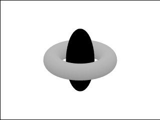
Figure 3: Ellipsoidal–Torus Configuration

The ellipsoidal–torus configuration is illustrated in Fig. 3.

We can consider different combinations of ellipsoidal black hole an black torus metrics in order to construct solutions of Class AA, AB and BB (we omit such similar constructions).

IV.2.2 A second example of ellipsoidal black hole – black torus system

In the simplest case we can construct a solution with an ellipsoidal and toroidal horizon which have a trivial conformal factor $\Omega$ and vanishing coefficients $\zeta_{i}=0$ (see (31)). Establishing a global 3D toroidal space coordinate system, we consider the ansatz

$$\delta s^{2} = \{-\left[d\sigma^{2}+d\tau^{2}\right]-\eta_{3}\left(\sigma,\tau,\varphi\right)h_{3[0]}\left(\sigma,\tau\right)\delta\varphi^{2}$$

$$+\eta_{4}\left(\sigma,\tau,\varphi\right)h_{4[0]}\left(\sigma,\tau\right)\delta t^{2}\},$$

where (in order to construct a Class AA solution) we put

$$h_{3[0]} = a_{E}\left(\sigma,\tau\right)a_{T}\left(\sigma,\tau\right),h_{4[0]}=b_{E}\left(\sigma,\tau\right)b_{T}\left(\sigma,\tau\right),$$

$$\eta_{4} = \omega^{-2}\left(\sigma,\tau,\varphi\right)\varpi^{-2}\left(\sigma,\tau,\varphi\right),$$

considering anisotropic renormalizations of constants as in (32) and (40). The polarization $\eta_{3}$ is to be found from the relation

$$h_{3}=h_{[0]}^{2}[(\sqrt{|h_{4}|})^{\ast}]^{2},h_{[0]}^{2}=const,$$ (45)

which defines a soltuion of equation (27) for $h_{4}^{\ast}\neq 0$ , when $h_{3}=-\eta_{3}h_{3[0]}$ and $h_{4}=\eta_{4}h_{4[0]}.$ Substitutting the last values in (45) we get

$$|\eta_{3}|=h_{[0]}^{2}\frac{b_{E}b_{T}}{a_{E}a_{T}}\left(\frac{\omega^{\ast}+\varpi^{\ast}}{\omega\varpi}\right)^{2}.$$

Then, computing the coefficient $\gamma,$ see (29), after two integrations on $\varphi$ we find

$$n_{i}\left(\sigma,\tau,\varphi\right)=n_{i[0]}\left(\sigma,\tau\right)+n_{i[1]}\left(\sigma,\tau\right)\int[\eta_{3}/\left(\sqrt{|\eta_{3}|}\right)^{3}]d\varphi$$

$$=n_{i[0]}\left(\sigma,\tau\right)+\tilde{n}_{i[1]}\left(\sigma,\tau\right)\int\omega\varpi\left(\omega^{\ast}+\varpi^{\ast}\right)^{2}d\varphi,$$

where we re-defined the function $n_{i[1]}\left(\sigma,\tau\right)$ into a new $\tilde{n}_{i[1]}\left(\sigma,\tau\right)$ by including all factors and constants like $h_{[0]}^{2},$ $b_{E},b_{T},a_{E}$ and $a_{T}.$

The constructed solution (IV.2.2) does not has as locally isotropic limit the Schwarzschild metric. It has also a toroidal and ellipsoidal horizons defined by the conditions of vanishing of $b_{E}$ and $b_{T},$ but this solution is different from the metric (IV.2.1): it has a trivial conformal factor and vanishing coefficients $\zeta_{i}$ which means that in this case we are having a splitting of dynamics into three holonomic and one anholonomic coordinate. We can select such functions $n_{i[0,1]}\left(\sigma,\tau\right),$ $\omega\left(\sigma,\tau,\varphi\right)$ and $\varpi\left(\sigma,\tau,\varphi\right),$ when at asymptotics one obtains the Minkowski metric.

V Anisotropic Polarizations and Running Constants

In this Section we consider non–static vacuum anholonomic ellipsoidal and/or toroidal configurations depending explicitly on time variable $t$ and on holonomic coordiantes $x^{i},$ but not on angular coordinate $\varphi.$ Such solutions are generated by dynamical anholonomic deformations and conformal transforms of the Schwarzschild metric. For simplicity, we analyze only Class A and AA solutions.

The coordinates are parametrized: $x^{i}$ are holonomic ones, in particular, $x^{i}=\left(u,\lambda\right),$ for ellipsoidal configurations, and $x^{i}=\left(\sigma,\tau\right),$ for toroidal configurations; $y^{3}=v=t$ and $y^{4}=\varphi.$ The metric ansatz is stated in the form

$$\delta s^{2} = \Omega^{2}\left(x^{i},t\right)[-(dx^{1})^{2}-(dx^{2})^{2}$$ (46)

$$+h_{3}\left(x^{i},t\right)\delta t^{2}+h_{4}\left(x^{i},t\right)\delta\varphi^{2}],$$

where the differentials are elongated

$$d\varphi \rightarrow \delta\varphi=d\varphi+\zeta_{i}\left(x^{k},t\right)dx^{i},$$

$$dt \rightarrow \delta t=dt+n_{i}\left(x^{k},t\right)dx^{i}.$$

The ansatz (46) is related with some ellipsoidal and/ or toroidal anholonomic deformations of the Schwarzschild metric (see respectively, (II.1), (8), (11) and (II.2), (15), (18)) via time running renormalizations of ellipsoidal and toroidal constants (instead of the static ones, (32) and (40)),

$$\rho_{g}\rightarrow\widehat{\rho}_{g}=\omega\left(x^{k},t\right)\rho_{g},$$ (47)

and

$$\rho_{g}^{[t]}\rightarrow\widehat{\rho}_{g}^{[t]}=\varpi\left(x^{k},t\right)\rho_{g}^{[t]}.$$ (48)

As particular cases we shall consider trivial values $\Omega^{2}=1.$ The horizons of such classes of solutions are defined by the condition of vanishing of the coefficient $h_{3}\left(x^{i},t\right).$

V.1 Ellipsoidal/toroidal solutions with running constants

V.1.1 Trivial conformal factors, $\Omega^{2}=1$

The simplest way to generate a $t$–depending ellipsoidal (or toroidal) configuration is to take the metric (8) (or (15)) and to renormalize the constant as (47) (or (48)). In result we obtain a metric (46) with $\Omega^{2}=1,$ $h_{3}=\eta_{3}\left(x^{i},t\right)h_{3[0]}\left(x^{i}\right)$ and $h_{4}=h_{4[0]}\left(x^{i}\right),$ where

$$\eta_{3} = \omega^{-2}\left(u,\lambda,t\right),h_{3[0]}=b_{E}\left(u,\lambda\right),h_{4[0]}=a_{E}\left(u,\lambda\right),$$

$$(\eta_{3} = \varpi^{-2}\left(\sigma,\tau,t\right),h_{3[0]}=b_{T}\left(\sigma,\tau\right),h_{4[0]}=a_{T}\left(\tau\right)).$$

The equation (27) is satisfied by these data because $h_{4}^{\ast}=0$ and the condition (31) holds for $\zeta_{i}=0.$ The coefficient $\gamma$ from (29) is defined only by polarization $\eta_{3},$ which allow us to write the integral of (28) as

$$n_{i}=n_{i[0]}\left(x^{i}\right)+n_{i[1]}\left(x^{i}\right)\int\eta_{3}\left(x^{i},t\right)dt.$$

The corresponding ellipsoidal (or toroidal) configuration may be transformed into asymptotically Minkowschi metric if the functions $\omega^{-2}\left(u,\lambda,t\right)$ (or $\varpi^{-2}\left(\sigma,\tau,t\right))$ and $n_{i[0,1]}\left(x^{i}\right)$ are such way determined by boundary conditions that $\eta_{3}\rightarrow const$ and $n_{i[0,1]}\left(x^{i}\right)\rightarrow 0,$ far away from the horizons, which are defined by the conditions $b_{E}\left(u,\lambda\right)=0$ (or $b_{T}\left(\sigma,\tau\right)=0).$

Such vacuum gravitational configurations may be considered as to posses running of gravitational constants in a local spacetime region. For instance, in Ref v we suggested the idea that a vacuum gravitational soliton may renormalize effectively the constants, but at asymptotics we have static configurations.

V.1.2 Non–trivial conformal factors

The previous configuration can not be related directly with the Schwarzschild metric (we used  its conformal transforms). A more direct relation is possible if we consider non–trivial conformal factors. For ellipsoidal (or toroidal) configurations we renromalize (as in (47), or (48)) the conformal factor (10) (or (17)),

$$\Omega^{2}\left(x^{k},t\right) = \omega^{2}\left(x^{k},t\right)\Omega_{AE}^{2}(x^{k})b_{E}^{-1}\left(x^{k}\right),$$

$$(\Omega^{2}\left(x^{k},t\right) = \varpi^{2}\left(x^{k},t\right)\Omega_{AT}^{2}(x^{k})b_{T}^{-1}\left(x^{k}\right)).$$

In order to satisfy the condition (30) we choose $h_{3}=\Omega^{-2}$ but $h_{4}=h_{4[0]}$ as in previous subsection: this solves the equation (27). The non–trivial values of $\zeta_{i}$ and $n_{i}$ are defined from (31) and (28),

$$\zeta_{i}\left(x^{k},t\right) = \left(\Omega^{\ast}\right)^{-1}\partial_{i}\Omega,$$

$$n_{i}\left(x^{k},t\right) = n_{i[0]}\left(x^{k}\right)+n_{i[1]}\left(x^{k}\right)\int h_{3}\left(x^{i},t\right)dt.$$

We note that the conformal factor $\Omega^{2}$ is singular on horizon, which is defined by the condition of vanishing of the coefficient $h_{3},$ i. e. of $b_{E}$ (or $b_{T}$). By a corresponding parametrization of functions $\omega^{2}\left(x^{k},t\right)$ (or $\varpi^{2}\left(x^{k},t\right))$ and $n_{i[0,1]}\left(x^{k}\right)$ we may generate asymptotically flat solutions, very similar to the Schwarzschild solution, which have anholonomic running constants in a local region of spacetime.

V.2 Black Elipsoid – Torus Metrics with Running Constants

Now we consider nonlinear superpositions of the previous metrics as to construct solutions with running constants and two horizons (one ellipsoidal and another toroidal).

V.2.1 Trivial conformal factor, $\Omega^{2}=1$

The simplest way to generate such metrics with two horizons is to establish, for instance, a common toroidal system of coordinate, to take the ellipsoidal and toroidal metrics constructed in subsection V.A.1 and to multiply correspondingly their coefficients. The corresponding data, defining a new solution for the ansazt (46),  are

$$g_{1,2} = -1,\widehat{\rho}_{g}=\omega\left(x^{k},t\right)\rho_{g},\widehat{\rho}_{g}^{[t]}=\varpi\left(x^{k},t\right)\rho_{g}^{[t]},\Omega=1,$$

$$h_{3} = \eta_{3}\left(x^{i},t\right)h_{3[0]}\left(x^{i}\right),\eta_{3}=\omega^{-2}\left(x^{k},t\right)\varpi^{-2}\left(x^{k},t\right),$$

$$h_{3[0]} = b_{E}\left(x^{k}\right)b_{T}\left(x^{k}\right),h_{4}=h_{4[0]}=a_{E}\left(x^{i}\right)a_{T}(x^{i}),($$

$$\zeta_{i} = 0,n_{i}=n_{i[0]}\left(x^{k}\right)+n_{i[1]}\left(x^{k}\right)\int\omega^{-2}\varpi^{-2}dt,$$ (49)

where the functions $a_{E},a_{T}$ and $b_{E},b_{T}$ are given by formulas (9) and (16). Analyzing the data (49) we conclude that we have two horizons, when $b_{E}\left(x^{k}\right)=0$ and $b_{T}\left(x^{k}\right)=0,$ parametrized respectively as ellipsoidal and torus hypersurfaces. The boundary conditions on running constants and on off–diagonal components of the metric may be imposed as the solution would result in an asymptotic flat metric. In a finite region of spacetime we may consider various dependencies in time.

V.2.2 Non–trivial conformal factor

In a similar manner, we can multiply the conformal factors and coefficients of the metrics from subsection V.A.2 in order to generate a solution parametrized by the (46) with nontrivial conformal factor $\Omega$ and non-vanishing coefficients $\zeta_{i}.$ The data are

$$g_{1,2} = -1,\widehat{\rho}_{g}=\omega\left(x^{k},t\right)\rho_{g},\widehat{\rho}_{g}^{[t]}=\varpi\left(x^{k},t\right)\rho_{g}^{[t]},$$ (50)

$$\Omega^{2} = \omega^{2}\left(x^{k},t\right)\varpi^{2}\left(x^{k},t\right)\Omega_{AE}^{2}(x^{k})\times$$

$$\Omega_{AT}^{2}(x^{k})b_{E}^{-1}\left(x^{k}\right)b_{T}^{-1}\left(x^{k}\right),(\mbox{ see (\ref{auxm1s}),(\ref{auxm1tb})}),$$

$$h_{3} = \Omega^{-2},h_{3[0]}=b_{E}\left(x^{k}\right)b_{T}\left(x^{k}\right),$$

$$h_{4} = h_{4[0]}=a_{E}\left(x^{i}\right)a_{T}(x^{i}),\zeta_{i}\left(x^{k},t\right)=\left(\Omega^{\ast}\right)^{-1}\partial_{i}\Omega,$$

$$n_{i} = n_{i[0]}\left(x^{k}\right)+n_{i[1]}\left(x^{k}\right)\int\omega^{-2}\varpi^{-2}dt.$$

The data (50) define a new type of solution than that given by (49). It this case there is a singular on horizons conformal factor. The behaviour nearly horizons is very complicated. By corresponding parametrizations of functions $\omega\left(x^{k},t\right),$ $\varpi\left(x^{k},t\right)$ and $n_{i[0,1]}\left(x^{k}\right),$ which approximate $\omega,\varpi\rightarrow const$ and $\zeta_{i},n_{i}\rightarrow 0$ we may obtain a stationary flat asymptotics.

Finally, we note that instead of Class AA solutions with anisotropic and running constants we may generate solutions with two horizons (ellipsoidal and toroidal) by considering nonlinear superpositions, anholonomic deformations, conformal transforms and combinations of solutions of Classes A, B. The method of construction is similar to that considered in this Section.

VI Conclusions and Discussion

We constructed new classes of exact solutions of vacuum Einstein equations by considering anholonomic deformations and conformal transforms of the Schwarzshild black hole metric. The solutions posses ellipsoidal and/ or toroidal horizons and symmetries and could be with anisotropic renormalizations and running constants. Some of such solutions define static configurations and have Schwarzschild like (in general, multiplied to a conformal factor) asymptotically flat limits. The new metrics are parametrized by off–diagonal metrics which can be diagonalized with respect to certain anholonomic frames. The coefficients of diagonalized metrics are similar to the Schwazschild metric coefficients but describe deformed horizons and contain additional dependencies on one ’anholonomic’ coordinate.

We consider that such vacuum gravitational configurations with non–trivial topology and deformed horizons define a new class of ellipsoidal black hole and black torus objects and/or their combinations.

Toroidal and ellipsoidal black hole solutions were constructed for different models of extra dimension gravity and in the four dimensional (4D) gravity with cosmological constant and specific configurations of matter lemos ; rev ; emp . There were defined also vacuum configurations for such objects v ; v2 ; vth ; vtor . However, we must solve the very important problems of physical interpretation of solutions with anholonomy and to state their compatibility with the black hole uniqueness theorems israel and the principle of topological censorship haw ; cen .

It is well known that the Scwarzschild metric is no longer the unique asymptotically flat static solution if the 4D gravity is derived as an effective theory from extra dimension like in recent Randall and Sundrum theories (see basic results and references in rs ). The Newton law may be modified at sub-millimeter scales and there are possible configurations with violation of local Lorentz symmetry csaki . Guided by modern conjectures with extra dimension gravity and string/M–theory, we have to answer the question: it is possible to give a physical meaning to the solutions constructed in this paper only from a viewpoint of a generalized effective 4D Einstein theory, or they also can be embedded into the framework of general relativity theory?

It should be noted that the Schwarzschild solution was constructed as the unique static solution with spherical symmetry which was connected to the Newton spherical gravitational potential $\sim 1/r$ and defined as to result in the Minkowski flat spacetime, at long distances. This potential describes the static gravitational field of a point particle with ”isotropic” mass $m_{0}.$ The spherical symmetry is imposed at the very beginning and it is not a surprising fact that the spherical topology and spherical symmetry of horizons are obtained for well defined states of matter with specific energy conditions and in the vacuum limits. Here we note that the spherical coordinates and systems of reference are holonomic ones and the considered ansatz for the Schwarzschild metric is diagonal in the more ”natural” spherical coordinate frame.

We can approach in a different manner the question of constructing 4D static vacuum metrics. We might introduce into consideration off–diagonal ansatz, prescribe instead of the spherical symmetry a deformed one (ellipsoidal, toroidal, or their superposition) and try to check if a such configurations may be defined by a metric as to satisfy the 4D vacuum Einstein equations. Such metrics were difficult to be found because of cumbersome calculus if dealing with off–diagonal ansatz. But the problem was substantially simplified by an equivalent transferring of calculations with respect to anholonomic frames v ; vth ; vtor . Alternative exact static solutions, with ellipsoidal and toroidal horizons (with possible extensions for nonlinear polarizations and running constants), were constructed and related to some anholonomic and conformal transforms of the Schwarzschild metric.

It is not difficult to suit such solutions with the asymptotic limit to the locally isotropic Minkowschi spacetime: ”an egg and/or a ring look like spheres far away from their non–trivial horizons”. The unsolved question is that what type of modified Newton potentials should be considered in this case as they would be compatible with non–spherical symmetries of solutions? The answer may be that at short distances the masses and constants are renormalized by specific nonlinear vacuum gravitational interactions which can induce anisotropic effective masses, ellipsoidal or toroidal polarizations and running constants. For instance, the Laplace equation for the Newton potential can be solved in ellipsoidal coordinates ll : this solution could be a background for constructing ellipsoidal Schwarzshild like metrics. Such nonlinear effects should be treated, in some approaches, as certain quasi–classical approximations for some 4D quantum gravity models, or related to another type of theories of extra dimension classical or quantum gravity.

Independently of the type of little, or more, internal structure of black holes with non–spherical horizons we search for physical justification, it is a fact that exact vacuum solutions with prescribed non–spherical symmetry of horizons can be constructed even in the framework of general relativity theory. Such solutions are parametrized by off–diagonal metrics, described equivalently, in a more simplified form, with respect to associated anholonomic frames; they define some anholonomic vacuum gravitational configurations of corresponding symmetry and topology. Considering certain characteristic initial value problems we can select solutions which at asymptotics result in the Minkowschi flat spacetime, or into an anti–de Sitter (AdS) spacetime, and have a causal behaviour of geodesics with the equations solved with respect to anholonomic frames.

It is known that the topological censorship principle was reconsidered for AdS black holes cen . But such principles and uniqueness black hole theorems have not yet been proven for spacetimes defined by generic off–diagonal metrics with prescribed non–spherical symmetries and horizons and with associated anholonomic frames with mixtures of holonomic and anholonomic variables. It is clear that we do not violate the conditions of such theorems for those solutions which are locally anisotropic and with nontrivial topology in a finite region of spacetime and have locally isotropic flat and trivial topology limits. We can select for physical considerations only the solutions which satisfy the conditions of the mentioned restrictive theorems and principles but with respect to well defined anholonomic frames with holonomic limits. As to more sophisticate nonlinear vacuum gravitational configurations with global non–trivial topology we conclude that there are required a more deep analysis and new physical interpretations.

The off–diagonal metrics and associated anholonomic frames extend the class of vacuum gravitational configurations as to be described by a nonlinear, anholonomic and anisotropic dynamics which, in general, may not have any well known locally isotropic and holonomic limits. The formulation and proof of some uniqueness theorems and principles of topological censorship as well analysis of physical consequences of such anholonomic vacuum solutions is very difficult. We expect that it is possible to reconsider the statements of the Israel–Carter–Robinson and Hawking theorems with respect to anholonomic frames and spacetimes with non–spherical topology and anholonomically deformed spherical symmetries. These subjects are currently under our investigation.

Acknowledgements

Figure 1: Ellipsoidal Configuration

References

• (1) M. H. P. M. van Putten, Phys. Rev. Lett.  84  (2000) 3752; Gravitational Radiation From a Torus Around a Black Hole, astro-ph/ 0107007; R. M. Wald, Phys. Rev. D10 (1974) 1680; Dokuchaev V. I. Sov. Phys. JETP 65 (1986) 1079.
• (2) J.P.S. Lemos, Class. Quant. Grav.  12 , (1995) 1081; Phys. Lett. B 352 (1995) 46; J.P.S. Lemos and V. T. Zanchin, Phys. Rev. D54 (1996) 3840; P.M. Sa and J.P.S. Lemos, Phys. Lett. B423(1998) 49; J.P.S. Lemos, Phys. Rev. D57 (1998) 4600; Nucl. Phys. B600 (2001) 272.
• (3) R. B. Mann, in Internal Structure of Black Holes and Spacetime Singularities, eds. L. Burko and A. Ori, Ann. Israely Phys. Soc. 13 (1998), 311.
• (4) S. Vacaru, JHEP 0104 (2001) 009; S. Vacaru, Locally Anisotropic Black Holes in Einstein Gravity, gr–qc/ 0001020.
• (5) S. Vacaru,  Ann. Phys. (NY) 290, 83 (2001); Phys. Lett. B 498 (2001) 74; S. Vacaru, D. Singleton, V. Botan and D. Dotenco, Phys. Lett. B 519 (2001) 249; S. Vacaru and F. C. Popa, Class. Quant. Grav.  18 (2001) 4921-4938, hep-th/0105316.
• (6) A. Chamblin and R. Emparan, Phys. Rev. D55 (1997) 754; R. Emparan, Nucl. Phys.  B610  (2001) 169; M. I. Cai and G. J. Galloway, Class. Quant. Grav.  18 , (2001) 2707; R. Emparan and H. S. Reall, hep–th/ 0110258, hep-th/ 0110260.
• (7) S. Vacaru, A New Method of Constructing Black Hole Solutions in Einstein and 5D Gravity, hep-th/0110250; S. Vacaru and E. Gaburov, Anisotropic Black Holes in Einstein and Brane Gravity, hep-th/0108065.
• (8) S. Vacaru, Black Tori Solutions in Einstein and 5D Gravity, hep–th/0110284.
• (9) W. Israel, Phys. Rev. 164, 1776 (1967);  B. Carter, Phys. Rev. Lett 26, 331 (1971); D. C. Robinson, Phys. Rev. Lett 34, 905 (1975); M. Heusler, Black Hole Uniqueness Theorems (Cambridge University Press, 1996).
• (10) S. W. Hawking, Commun. Math. Phys. 25 (1972), 152.
• (11) G. J. Galloway, K. Seheich, D. M. Witt and E. Woolgar, Phys. Rev. D60 (1999) 104039.
• (12) L. Landau and E. M. Lifshits, The Classical Theory of Fields, vol. 2 (Nauka, Moscow, 1988) [in russian]; S. Weinberg,  Gravitation and Cosmology, (John Wiley and Sons, 1972).
• (13) G. A. Korn and T. M. Korn, Mathematical Handbook (McGraw–Hill Book Company, 1968).
• (14) L. Randall and R. Sundrum, Phys. Rev. Lett.  83  (1999) 3370; Phys. Rev. Lett.  83  (1999) 4690; T. Shiromizu, K. Maeda and M. Sasaki, Phys. Rev. D62 (2000) 0101059; R. Maartens, gr–qc/0101059.
• (15) C. Csaki, J. Erlich and C. Grojean, Nucl. Phys. bf b604 (2001) 312.
Refer to caption