An Holographic Cosmology

Abstract:

We present a new cosmological model, based on the holographic principle, which shares many of the virtues of inflation. The very earliest semiclassical era of the universe is dominated by a dense gas of black holes, with equation of state $p=\rho$. Fluctuations lead to an instability to a phase with a dilute gas of black holes, which later decays via Hawking radiation to a radiation dominated universe. The quantum fluctuations of the initial state give rise to a scale invariant spectrum of density perturbations, for a range of scales. We point out a problem , that appears to prevent the range of scales predicted by the model from coinciding with the range where such a spectrum has been observed. We speculate that this may be related to our field theoretic treatment of fluctuations in the highly holographic $p=\rho$ background. The monopole problem is solved in a manner completely different from inflationary models, and a relic density of highly charged extremal black monopoles is predicted. We discuss the nature of the entropy and flatness problems in our model.

1 Introduction

In a recent paper[1] we presented an introduction to a quantum theory of cosmology. The focus of this as yet incomplete formalism was the combination of the holographic principle with the conventional notion of particle horizon. The fact that these two concepts are compatible with each other was an important , though implicit, message of [3]. We used insights from this formalism to begin the construction of a semiclassical cosmology, which would be compatible with the basic principles of M-theory. We argued that the earliest semiclassical era of the universe consisted of a homogeneous gas with equation of state $p=\rho$, which saturates the F(ischler)-S(usskind)-B(ousso) entropy bound. We pointed out that this provided a noninflationary solution of the horizon problem. That is, a homogeneous gas can carry the entire entropy allowed by the holographic bound, so there are no significant inhomogeneous perturbations of the system.

In this paper we show that a dense gas of black holes, one in which the typical black hole size is of order the particle horizon, and the typical distance between black holes is of order their Schwarzchild radius, provides a picturesque physical realization of the $p=\rho$ gas. This description allows us to obtain a crude picture of the evolution of the universe. We argue that, apart from quantum and statistical fluctuations, the $p=\rho$ state is stable. Black holes merge to form a single horizon sized black hole as the universe expands. However, quantum mechanically, there is a nonzero probability that some horizon volumes have smaller than average black holes in them. If the black holes in a sufficient number of contiguous horizon volumes are small enough, they cease to merge, and evolve as a $p=0$ gas. The primordial black holes decay rapidly and produce small radiation dominated regions. These regions grow in physical volume, more rapidly than the $p=\rho$ background and after some time the universe consists of large $p={1\over 3}\rho$ regions with black holes (the remnants of the $p=\rho$ phase) caught in the interstices between them. The coarse grained universe is thus described by a nonrelativistic gas of large black holes. There is also likely to be a large $p=\rho$ region outside the combined particle horizons of the $p=\rho/3$ region. We will refer to the $p=\rho$ regime as the dense black hole fluid, and the $p=\rho/3$ regime as the dilute black hole gas.

The dilute black hole gas regions evolve like a conventional matter dominated cosmology. However, the black holes which comprise the non relativistic matter are unstable to decay via Hawking radiation. When these black holes decay the universe becomes radiation dominated. The largest black holes are those caught in the interstices between different $p=\rho/3$ regions, rather than incorporated within any one original region. These dominate the energy density until the time they decay.

The fluctuations in the distribution of matter in the $p=\rho/3$ regions are thus the fluctuations in the distribution of these largest black holes. We argue that at very large length scales, these fluctuations are determined by the quantum fluctuations in the original distribution of $p=\rho/3$ regions in the $p=\rho$ gas. We make the hypothesis that the form of these quantum fluctuations at large scale is calculable in terms of quantum field theory and comes predominantly from the long range two point correlations of the gravitational field . The large scale fluctuations are thus Gaussian. We further show that in the $p=\rho$ background, they are scale invariant: the magnitude of fluctuations at the horizon scale is independent of how large the horizon scale is. Standard arguments show that once these quantum fluctuations have been converted into classical matter density fluctuations, this scale invariance persists and will show up in the cosmic microwave spectrum.

Two crucial assumptions in the above discussion of fluctuations are that the initial density of dilute black hole gas regions is small and that the fluctuations of this distribution around its average are even smaller. We argue that both these facts are consequence of the low probability $P_{0}$ of finding dilute gas regions large enough to destabilize the dense black hole fluid. The small initial density of dilute gas regions implies that the dense black hole fluid persists for a considerable time. This has two important consequences. It contributes to the solution of the monopole problem, by a mechanism adumbrated below, and it determines the reheat temperature of the universe. The fundamental parameter $P_{0}$ appears to be determined by Planck scale physics, for reasons we will explain below.

Our quantum cosmology thus provides a mechanism for producing a homogeneous isotropic universe with a spectrum of small, Gaussian, scale invariant, fluctuations. However, we argue that causality constraints on our quantum field theoretic formalism imply that the largest scale for which we predict a scale invariant spectrum is $10^{7}$ times smaller than the current horizon radius. This suggests that (either our model is wrong or) our field theoretic treatment of the dense black hole gas is an inadequate description of this highly holographic system. In the conclusions we will speculate about how a proper quantum treatment of this regime might remove the discrepancy that we have found.

We will argue that our model provides insight into the other cosmological conundra that inflation was invented to solve. Briefly, the monopole problem is solved because monopoles originate as magnetically charged black holes. There is a small entropic suppression of such black holes. However, the major part of the resolution of the monopole problem comes from the length of time spent in the $p=\rho$ era. During this period, black holes are growing via mergers. Since the era lasts for a long time, they are quite massive by the time the universe becomes matter dominated (for the first time). They also develop a very large charge. The magnetically charged black holes will remain as remnants and will evolve into extremal magnetic black holes with huge charge. We will call these remnants, and their nonextremal progenitors, black monopoles.

Hawking decay of both charged and neutral black holes produces a large number of photons per monopole. For a sufficiently long $p=\rho$ era, the monopole to photon ratio is small enough to satisfy all known bounds. In contrast to the inflationary scenarios, our cosmology might produce an observable relic density of monopoles. Furthermore, the relic black monopoles are exotic and have extremely large charge.

Another problem whose resolution is credited to inflation is the entropy problem. We have often been confused by statements of this problem in the literature. Many of them are mathematically equivalent to the following fact: the linear size of our present horizon volume, at the era when the energy density approaches the Planck scale, is $10^{29}$ in Planck units. In our view, this large number reflects the holographic bounds and the total number of quantum states of the universe.

The number of quantum states in the universe is determined by the cosmological constant. Any geometrical description of the universe must then begin with a large spacetime, even at the Planck density. The precise way in which the available states are distributed between the cosmological horizon and more localized systems is determined by dynamics. The conventional count of the entropy of the universe includes only the localized entropy. In our model, this will be explained by detailed dynamical calculations.

Finally, we come to the flatness problem, whose resolution is one of the phenomenological triumphs of inflation. Our viewpoint on this is unorthodox. We are tempted to view the problem as resulting from an unjustified use of homogeneous isotropic cosmology to describe the very early universe, an improper mingling of phenomenology and fundamental theory. Indeed, the horizon problem tells us that homogeneous isotropic cosmology should be derived rather than postulated and this is the case in our model. We will provide dynamical justification for flatness within a horizon volume at early times, and we believe that this is enough to account for observations. More global requirements of flatness seem unjustified to us. Small deviations from the flat background geometry in each horizon volume have no reason to be aligned to produce an average curvature. Rather, they should be viewed as random fluctuations in spatial curvature, which, using Einstein’s equations, are equivalent to density fluctuations. We will calculate these fluctuations in our model, and they do not give rise to an average curvature.

In the course of our discussion of black monopole evaporation, we will note that these processes provide an unconventional source of baryon asymmetry, whose order of magnitude is hard to calculate. We will also find indications, though no firm argument, that the reheat temperature of the universe is very low, so that many conventional methods of producing baryon asymmetry will not be applicable. Affleck-Dine [14] coherent baryogenesis would be the leading candidate mechanism, unless the asymmetry generated in black monopole interactions and decay is sufficient. We will also make some brief comments about gravitinos, axions, and dark matter.

To summarize the plan of this paper: Section 2 is the heart of the paper and fills in the sketch we have presented above. Section 3 is devoted to a short critique of inflationary models in view of the nonzero value of the cosmological constant, and a comparison of such models with our own. It also contains our conclusions.

Before proceeding, a word about the relation of our work to M-theory. This rubric currently applies to a collection of supersymmetric vacuum states with Poincare or Anti-deSitter SUSY. There are plausible arguments for SUSY violating vacua with AdS symmetry, as well as SUSY violating, weakly coupled, string cosmologies with no cosmological horizon. We believe that all of these can be viewed as limits of a more general structure whose basic rules will incorporate and make precise the Holographic Principle[4], and the UV/IR connection[5]. Apart from a brief remark that higher dimensional physics is important for the determination of the parameters $P_{0}$ and $M_{0}$ defined below, our cosmological model will employ only these two fundamental principles of M-theory.

2 Semiclassical cosmology

The considerations of [1] motivate us to choose a time slicing of spacetime such that all backward light cones with their tips on a given time slice, have the same FSB area. Once this area is large enough, we expect to be able to describe much of the physics in terms of a background spacetime, and localized fluctuations in it. Let $H_{0}$ be the Hubble parameter at the first instant at which we believe semiclassical geometry (but not quantum field theory) is a good approximation. $H_{0}^{-1}$ must be larger than the Planck scale; precisely how large is not clear. For brevity, we will refer to this first semiclassical time slice as the initial instant in the remainder of the text. Locally, within a backward light cone ending on this time slice, it makes sense to view the universe as an FRW space with some sort of localized excitations in it. This defines a Hamiltonian time evolution according to the FRW time. The question is, what should we take for the initial state? In our previous paper we argued that this should be a fluid with $p=\rho$, because such a fluid dominates the energy density at small scale factor, and is the only homogeneous fluid that can saturate the FSB entropy bounds for all times. We will begin by choosing a flat FRW space, and then discuss other options.

It does not make sense to search for low energy states of the FRW Hamiltonian. Prior to this time, this particular choice of time evolution did not make any sense. It is only well defined in the semiclassical regime[6]. Rather, we should choose a generic initial state, consistent with the fact that it is contained in our backward light cone. Here, the UV/IR connection of M-theory comes in handy. It assures us that the density of states grows rapidly at very high FRW energy, and that the high energy states all have the geometry of black holes. We do not have a good microscopic description of these states from the point of view of an observer who hovers outside the black hole, but a loose application of the No-Hair theorem assures us that they all have the same macroscopic geometry for given values of charge, mass and angular momentum.

It is important to note that black holes are really only defined in terms of asymptotic geometry. We are thinking of black holes inside a backward light cone as regions bounded by an apparent horizon of a certain area. Our discussion of their properties is only approximate. It is clear what we mean by such a black hole in the limit that its radius is small compared to the horizon size. That is, it looks like a portion of the Schwarzchild metric. As we scale up the black hole mass we have to take into account the presence of black holes in other horizon volumes. More importantly, we need to take cognizance of the fact that our statistical arguments for the most likely state apply to all backward light cones, including those that overlap partially with each other. Geometrically, it is inconsistent to insist on a configuration, which is simultaneously spherically symmetric around the centers of two overlapping light cones. For the purposes of the present paper we will need to assume only two properties of the ”scaled up black holes” . The first is that the energy/entropy/size scalings of small black hole configurations can be extrapolated to the regime where the black hole and particle horizons have comparable scale. The second is that the geometrical features of the scaled up black holes remain independent of their internal state. The horizon problem is solved by the claim that geometry is a “thermodynamic” property of the generic state of a large black hole.

Indeed, we suspect that there is no consistent geometrical description of the microstructure of the dense black hole gas. Only its coarse grained FRW geometry makes sense. Geometrical features have operational meaning only when the system has particle (or extended object) degrees of freedom which propagate locally in the geometry. Starting from a picture of small black holes in each horizon volume we see that the space available for such propagation gets smaller as we scale up the black hole mass. In the limit of a dense black hole gas, a would be particle emitted from one black hole is immediately absorbed by another. There would seem to be no localized excitations of this fluid, which is perhaps another way of understanding why it solves the horizon problem.

The reader who absorbs and believes these arguments will have a hard time making them consistent with our later use of field theory to calculate fluctuations in the dense black hole fluid. We are in complete sympathy with such skepticism, and believe that it may explain why our calculation, although it obtains the right power law, is not consistent with observation. We will show that the causality bounds of field theory (no correlation between events that have not had time to communicate through light signals) prevent us from applying our spectrum calculation to the scales at which a Harrison-Zeldovitch spectrum has been observed in the universe. We will emphasize that our calculation depends only on scaling properties of the $p=\rho$ FRW metric. We hope that these scaling properties may survive a proper treatment of fluctuations in the $p=\rho$ fluid, but that the field theoretic causality bounds will be circumvented.

To summarize, if we consider a set of disjoint backward light cones ending on our time slice, then, to the extent that the horizon is large so that the spectrum of allowed black holes is strongly peaked at the maximal size, observers in each of these light cones will see the same geometry with high probability. Note that all of the dominant fluctuations away from this most probable situation will consist of (collections of) smaller black holes.

Now let us argue that such a collection of maximal black holes behaves like a $p=\rho$ fluid. We will do this in arbitrary dimension, and write the equations in Planck units appropriate to the dimension in which we are working. Let $n$ be the number density of black holes in comoving coordinates and $M$ be their mass. The energy density is

$$\rho=Mn$$ (1)

while the entropy density is

$$\sigma=M^{{d-2\over d-3}}n$$ (2)

The black holes are all of the scale of the horizon:

$$R_{S}\sim M^{1\over d-3}\sim H_{0}^{-1}$$ (3)

Since there is one such black hole in each horizon volume, we have $n\sim R_{S}^{-(d-1)}$

Thus

$$\rho\sim R_{S}^{-2}$$ (4)

$$\sigma\sim R_{S}^{-1}\sim\sqrt{\rho}$$ (5)

This is the energy/entropy relation of a $p=\rho$ fluid. To really claim that we have such an equation of state we must show that the postulated configuration of horizon filling black holes is stable over a reasonably long period. To see what this entails note that with the $p=\rho$ equation of state, when the universe expands by a scale factor $A$, then $\sigma\sim A^{-(d-1)}\sim\rho^{1/2}$. Using the black hole formulae, this implies that $n\sim A^{-(d-1)^{2}}$. If the black hole number were conserved we would have $n\sim A^{-(d-1)}$ so $A^{(d-1)(d-2)}$ black holes must merge to form a single horizon filling black hole as the universe expands, if the black hole fluid is to give $p=\rho$.

We believe that the dense black hole fluid is classically stable. That is, as black holes come into each other’s horizon volume they are only a Schwarzchild radius apart and will merge in less than an e-folding time of the universe. However, we should remember that our claim that the state in each light cone was a maximal size black hole is only statistical. There is some probability that it will be a collection of smaller black holes. If there is a region of contiguous horizon volumes filled with sufficiently small black holes then they will not merge as the horizon expands. In such a region the black holes will behave like a $p=0$ gas. Thus, the initial state of the universe is a dense black hole fluid with a few dilute areas where the equation of state is $p=0$. Since these small black holes will evaporate quickly, the equation of state in these regions quickly becomes that of a relativistic gas. In a coarse grained view, averaging over many initial horizon volumes, we have a two component homogeneous fluid.

The dilute black hole/radiation gas component has an initial density much smaller than the dense black hole fluid component, because the probability of finding a large enough dilute region to prevent mergers is small. This is a consequence of the fact that in each horizon volume, the probability for finding any given configuration is sharply peaked at the maximal size black hole, because of the nature of the black hole entropy function. Furthermore, if we choose a configuration too close to the maximum then it will not evolve as a $p=0$ or relativistic gas. Indeed, imagine some collection of less than maximal black holes in a few connected horizon volumes. As the universe expands these black holes will be attracted to the maximal black holes in neighboring horizon volumes. If the infall time is short compared to the e-folding time in the putative $p=0$ region, then in fact the $p=0$ equation of state is never achieved. The matter originally in submaximal black holes will be absorbed into the dense black hole gas, and the empty region will cease expanding and will become a microscopic blip in the expanding $p=\rho$ universe. Causal processes will soon fill it with $p=\rho$ fluid. Since the energy density in the $p=0$ region must initially be less than that in the $p=\rho$ region, we can only achieve the $p=0$ equation of state if a fairly large number of contiguous horizon volumes simultaneously contain submaximal black holes.

On the contrary, if the entropy density of the fluctuation is sufficiently small then the fluctuation region will expand (initially according to the $p=0$ equation of state, and then like $p=\rho/3$) more rapidly than the surrounding $p=\rho$ fluid. We will consider its subsequent fate in a moment.

The fact that a finite gap from the maximal entropy is necessary in order to produce a fluctuation which can grow, means that the probability for such fluctuations is exponentially small in the region of validity of the semiclassical entropy formula. Indeed, if the entropy of the maximal black hole is $S_{max}$ then we expect that the probability for a growing bubble will behave like

$$P_{0}=e^{-NS_{max}}$$ (6)

The quantity $N$ is the number of contiguous horizon volumes which must simultaneously have submaximal black holes. To do a proper calculation one would have to test many multi black hole configurations, to find the one which maximized the entropy among all those that succeeded in breaking away from the $p=\rho$ fluid. Furthermore, it is clear that fluctuations produced closer to the initial time slice are exponentially more probable than those produced later. Thus, the only important dilute regions are those produced at the initial instant. Indeed, it is likely that the correct calculation of $P_{0}$ cannot be done within the semiclassical approximation, since the semiclassical entropy formulae suggest that the probability is maximized at the point where the formulae break down. However, since the calculation always involves the joint probability for a number of low probability events, the result is guaranteed to be small. Thus, we will not attempt a calculation of $P_{0}$, but will believe the strong suggestion of the semiclassical approximation, that it is very small.

The considerations that determine $P_{0}$ and the dominant configuration which breaks away from the $p=\rho$ expansion are translation invariant, and the local probability distribution is strongly peaked around the maximum. Thus we expect the distribution of dilute black hole spheres in the dense fluid background to be uniform, with small fluctuations. To get some idea of how the fluctuations behave locally, consider a toy model in which the dominant breakway configuration is a distribution of $K$ black holes of mass $m<M_{max}$, and consider fluctuations $m\rightarrow m-\delta m$. $\delta m$ is presumed to be positive because any mass larger than $m$ would be reabsorbed into the $p=\rho$ fluid. For simplicity we will write formulae in $4$ spacetime dimensions. The (unnormalized) probability distribution for $\delta m$ is

$$P(\delta m)\sim e^{-8\pi Km\ \delta m}$$ (7)

.

If $m$ is large in Planck units, the fluctuations are of order $1/8\pi Km$; small but not exponentially small.

It is clear then that the inhomogeneous fluctuations in the distribution of $p=0$ spheres are suppressed by the same mechanism that makes the density of such spheres small. By the same token, it is difficult to perform a reliable calculation of the precise amplitude of the fluctuations. It is determined by Planck scale physics. We will come back to discuss the spatial variation of the correlation function of these fluctuations after we have established that it determines our model’s prediction for the fluctuations in the cosmic microwave background and for perturbations that give rise to galaxies and other large scale structures.

The above discussion suggests that our investigation must begin at a time when all the dimensions of the universe are in play. This is indeed true, but we will see that higher dimensional physics has only a small effect on our results. First of all we must state our hypothesis that the M-theory vacuum that is relevant for the universe is isolated and that the moduli are frozen at a very high scale. This sort of scenario has long been advocated by M. Dine [7] and has many attractions. We adopt it both because the alternative is more complicated (and we have not worked it out) and because it is implied by the hypothesis of cosmological SUSY breaking[9]. If we use $M_{d}$ as a symbol for the higher dimensional Planck mass, our hypothesis is that the moduli are fixed at a SUSY minimum of a potential whose typical scale is at least of order $M_{d}^{6}/M_{P}^{2}$ (here, because of the obvious ambiguity, we relax our convention that any Planck mass is unity).

The most obvious phenomenological reason to hypothesize compact dimensions larger than $M_{d}^{-1}$ is so that one can implement Witten’s explanation [10] of the discrepancy between the Planck mass and the unification scale. In the Horava-Witten scenario [11], where the internal manifold is highly anisotropic, this implies a maximal Kaluza-Klein radius of order $70$ times $M_{d}^{-1}$. In hypothetical scenarios in which the standard model arises from a codimension $4$ singularity in a $G_{2}$ manifold [12] the coefficient $70$ would be replaced by a smaller number. Of course, in recent years we have seen a large number of models with much larger internal dimensions. We will see below that such models are problematic in our framework.

Let us thus begin our discussion of the $p=\rho$ phase in $11$ dimensions (we choose $11$ rather than $10$ for concreteness). The mass of a black hole constituent of the $p=\rho$ fluid must be taken larger than $M_{d}$ in order to justify our use of classical general relativity in its description. It grows like $a^{10}$ as the universe expands. Almost immediately, its Schwarzchild radius becomes as large as the largest $KK$ radius. The considerations of Gregory and LaFlamme [13] then show us that the entropy of eleven dimensional black holes is swamped by that of black branes wrapped around the compact manifold. It is eminently plausible (and truly the only coherent hypothesis we can make about this highly nonclassical era) that there is a transition to a four dimensional $p=\rho$ fluid. It no longer makes sense to talk about internal motions on the compact manifold, since they are (everywhere in four dimensional spacetime) hidden behind the horizon of the wrapped black branes. Within a few instants, then, the universe becomes a dense fluid of four dimensional black holes. Their initial mass $M_{0}$ is determined by the condition (in four dimensional Planck units)

$$2M_{0}\simeq R_{KK}$$ (8)

where we have chosen the largest dimension of the compact manifold as a measure of $R_{KK}$ (e.g. the Horava-Witten interval).

2.1 Fluctuations

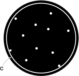
Figure 1: …

We are now ready to discuss the most important feature of any early universe cosmology, the nature of the density fluctuation spectrum at large scales. We will work in a synchronous coordinate system, in which we claim that the metric has the approximate form

$$ds^{2}=-dt^{2}+a^{2}({\bf x},t)d{\bf x}^{2}$$ (9)

We begin at the initial four dimensional slice. A two dimensional cartoon of the initial spatial configuration is given in Figure 1. The outer circle in this picture represents the fixed coordinate position of a presumed cosmological event horizon. Very little of what we have to say depends on this assumption of a nonzero value of the cosmological constant. The black region represents the dense gas of black holes, with equation of state $p=\rho$. The small white circles represent the spheres of dilute fluid, while the circle $C$ is just the boundary of the region where this finite number of spheres lie. The finiteness of the number of dilute spheres is a consequence of our assumption of a finite cosmological horizon. We will mostly discuss an approximation in which

$$a({\bf x},t)\approx a_{0}(t)\chi+a_{1}(t)(1-\chi)$$ (10)

where $\chi$ is the characteristic function of the region filled with white circles. Figure 1 is very far from being accurate as far as scale. The density of dilute regions, $P_{0}$, is extremely small. It is important to recognize that this statement remains true for all times. We are about to see that most of the physical volume of the universe becomes dominated by $p=0$ regions.

The coordinate size of the dilute spheres in the $p=\rho$ background is fixed. Since these regions are radiation dominated throughout most of their history, their physical size will grow like $t^{1/2}$. Thus we have to use a much finer coordinate grid in the dilute regions.

In any number of dimensions, in our gauge, the ratio of the volumes of $p={1\over 3}\rho$ and $p=\rho$ fluids at any time $t$ is

$$V_{1\over 3}=P_{0}\ t^{1\over 2}\ V_{1}$$ (11)

where $t=1$ is the initial time and $V_{w}$ is the physical volume of regions of $p=w\rho$ fluid. Thus, in Figure 1, the ratio of volumes of white circles to the entire black region is $P_{0}t_{d}^{1\over 2}$ where $t_{d}$ is the time between the initial instant and the Gregory-LaFlamme (GF)transition. $t_{d}$ is also, according to our general discussion of the $p=\rho$ fluid and its black hole interpretation, the ratio between the eleven dimensional black hole Schwarzchild radii at the GF transition and the initial instant.

If we assume an initial Schwarzchild radius close to $M_{d}^{-1}$, then $t_{d}$ is approximately $R_{KK}$ in $M_{d}^{-1}$ units. Thus, for compactifications of the type we have discussed $t_{d}$ is at most of order $100$. Since we have no reliable estimate of $P_{0}$, we might as well define

$$\bar{P}_{0}\equiv P_{0}t_{d}^{1\over 2}$$ (12)

Now let time evolve in four dimensions. The ratio between the physical volumes is $\bar{P}_{0}t^{1\over 2}$, while the mass of a black hole in the dense black hole fluid is $M_{0}t$. At the crossover time $t_{+}$, when $p=\rho/3$ regions begin to dominate the volume of the universe, the mass of black holes in the $p=\rho$ regions is $M_{0}/\bar{P}_{0}^{2}$.

We can draw a new cartoon of the situation by rescaling the size of the white circles by the ratio of volumes of the two fluids. We obtain Figure 2.

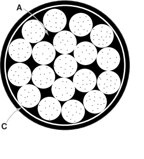
Figure 2: …

Actually, this figure also depicts the result of another physical process, which takes place as the $p=0$ volume begins to dominate. There are sheets of dense black hole fluid that are trapped between expanding $p=0$ spheres. Recall that the dense black hole fluid retains its equation of state by continual attraction and merger between its constituents. Obviously, the black holes in the sheets will not find any partners to merge with in the directions in which they encounter spheres of dilute black hole gas. The expanding spheres of dilute gas will leave interstices when they meet (e.g. the region marked A in Figure 2). The dense black hole fluid in these interstices can continue to merge and form larger and larger black holes. This interstitial fluid will attract the black holes in the sheets. We believe that all the $p=\rho$ fluid will accumulate in the interstices. The final situation (and this is what we depict in Figure 2.) will be a continuous region of dilute gas with spherical $p=\rho$ regions embedded in it. Each of these regions will eventually form a single large black hole, with mass of order $M\equiv M_{0}/\bar{P}_{0}^{2}$. The entire universe (inside $C$) will now be filled with a two component fluid. One component consists of the radiation produced in the decay of small black holes and the other of huge black holes with mass $M_{0}/\bar{P}_{0}^{2}$. The energy density is quickly dominated by the nonrelativistic gas of large black holes.

At this point Hawking evaporation of the large black holes comes into play. We can estimate the evaporation time of the large black holes, and the temperature to which they reheat the universe, by writing coupled equations for the black hole and radiation energy densities

$${d\rho_{BH}\over dt}=-3H\rho_{BH}-{1\over M^{3}}\rho_{BH}$$ (13)

$${d\rho_{\gamma}\over dt}=-4H\rho_{\gamma}+{1\over M^{3}}\rho_{BH}$$ (14)

$${dM\over dt}=-{1\over M^{2}}$$ (15)

$$H=\sqrt{\rho_{BH}+\rho_{\gamma}}$$ (16)

We have omitted all numerical constants from these equations since we are aiming only for order of magnitude results. Now notice that the rescalings

$$M\rightarrow bM$$ (17)

$$t\rightarrow b^{3}t$$ (18)

$$\rho_{BH,\gamma}\rightarrow b^{-6}\rho_{BH,\gamma}$$ (19)

leave these equations invariant. This enables us to see how the final photon energy density, and thus the reheat temperature, depends on the initial black hole mass $M_{0}/\bar{P}_{0}^{2}\equiv M$.

We obtain

$$T_{RH}\sim(M_{0}/\bar{P}_{0}^{2})^{-3/2}$$ (20)

This analysis also recovers the conventional estimate of the black hole evaporation time as $\sim M^{3}$.

A firm bound on the reheat temperature comes from nucleosynthesis:

$$T_{RH}>1MeV=10^{-22}M_{P}$$ (21)

One may also contemplate a stronger bound from the requirement of generating a baryon asymmetry. However, Affleck-Dine[14] (AD) baryogenesis seems to work at temperatures as low as an MeV. Furthermore, we will see below that our scenario presents us with a novel mechanism for baryogenesis , whose efficiency is difficult to estimate. Thus we will stick with the nucleosynthesis bound.

Any semiclassical estimate of $\bar{P}_{0}$ based on assuming the semiclassical entropy formula with black hole masses or Schwarzchild radii at least an order of magnitude above the relevant Planck scale gives a value of $\bar{P}_{0}$ that is completely incompatible with the nucleosynthesis bound. We have noted that the semiclassical formulae themselves suggest that $\bar{P}_{0}$ is determined by Planck scale physics and we don’t know how to estimate it. The above calculation is phenomenological testimony to the same fact.

In passing we note that the picture we have presented is incompatible with the idea of a very large KK radius. Whatever $\bar{P}_{0}$ is, it is certainly less than one, while $M_{0}$ is of order the largest KK radius. Thus, we find that $R_{KK}<10^{-18}cm$. Since we believe that $\bar{P}_{0}$ is probably quite small, this upper bound is probably a gross overestimate. Holographic cosmology does not seem to be compatible with very large KK radii.

On a more speculative note, let us consider the fact that in Figure 2, the region that will be identified with conventional cosmology is the interior of $C$.This sphere is surrounded by $p=\rho$ fluid that we can eventually think of as being ”squeezed up against the horizon”. It is tempting to identify this with the degrees of freedom on the horizon Indeed, the cosmological horizon is a holographic screen for the entire asymptotically deSitter space time. We use the gauge freedom available in the formalism discussed in [1] to project some of the degrees of freedom on local screens where more or less conventional low energy physics can be used to describe them. The rest of the states are associated with the horizon. Our picture suggests that these horizon states are remnants of a primordial $p=\rho$ fluid.

Indeed, the part of the $p=\rho$ gas outside the circle $C$ in Figure 1 interacts only very weakly with the local degrees of freedom that we describe in conventional cosmological language. Its degrees of freedom might as well be associated with the horizon. In this context it is worth remembering that if there is truly a cosmological constant of the order of magnitude indicated by measurements of distant supernovae[22], then the Bekenstein-Hawking entropy of the horizon is of order $10^{25}$ larger than the rest of the entropy of the visible universe (even if we include hypothetical $10^{6}$ solar mass black holes in each galaxy).

We have thus explored how our holographic cosmology produces an approximately homogeneous isotropic radiation dominated universe at temperatures of order $1$ MeV or above. We are now ready to calculate the form of fluctuations around the homogeneous state. The primordial fluctuations in matter density are those of the gas of large black holes caught in the interstices between $p=\rho/3$ regions. We have sketched the way in which the distribution of these black holes is determined by causal classical processes from the distribution of $p=\rho/3$ spheres in the $p=\rho$ background at the initial time. The latter fluctuations $\delta h({\bf x},t)$ should be thought of as fluctuations in the synchronous gauge metric. We have argued that they are likely to be small, though we have been unable to give a precise estimate of their magnitude. The result of the small size of $\delta h$ is that $\delta\rho$ is, to a good approximation, a linear functional of it:

$$\delta\rho({\bf x},t)=\int d^{3}ydsf({\bf x}-{\bf y},t,s)\delta h({\bf y},s)$$ (22)

$h$ is the trace part of the fluctuation in the synchronous gauge metric $\delta h^{i}_{j}$ with indices raised by the background $p=\rho$ metric. The transverse metric fluctuations represent gravitational waves. By causality of the classical physics that determines it, the function $f$ has a correlation length no larger than the coordinate horizon size at the end of the transition between $p=\rho$ and $p=\rho/3$ dominance. In fact, we believe that its Fourier transform goes to a constant at low comoving wavenumbers even when these waves have wavelength much smaller than this late time horizon. Crudely speaking, the position of a $p=\rho$ regions trapped in the interstices of the radiation dominated phase, is completely determined by the positions of a few near neighbor dilute regions at very early times. Thus $f$ should vary on the scale of the horizon at these very early times. Only dramatic motions of the bubbles of dilute fluid in the dense black hole background could give rise to correlations in $f$ over scales as large as the horizon at the phase transition. We do not see any reason why such motions occur. If this is correct, the complicated dynamics that fixes the large black hole positions in terms of the distribution of $p=0$ spheres, can affect the magnitude but not the shape of the fluctuation spectrum at low wave number.

To calculate the shape of the spectrum we recall that for observational purposes we are interested only in fluctuations of very long wavelength. Furthermore, we are working in a regime where the energy density is small compared to the Planck scale At very large wavelengths it is perhaps plausible that the correlations are well described by quantum field theory. Moreover, the dominant long distance correlations in field theory come from single particle exchange of massless particles.

Inflationary cosmology has taught us how such quantum fluctuations are converted into classical fluctuations once they enter the horizon. The wave function is a superposition of amplitudes for different classical distributions $\delta\rho_{0}({\bf x})$. Once a fluctuation is smaller than the horizon size it causes distortions in the background geometry, which in turn influence other degrees of freedom propagating in it. Since there are a large number of such degrees of freedom, phase correlations between different pieces of the wave function become irrelevant to the future evolution of the system. The different parts of the wave function that produce macroscopically different classical geometries ”decohere” and quantum mechanics gives rise to an inhomogeneous universe whose inhomogeneities can only be predicted statistically. The basic mechanism is in no way tied to inflation, and is applicable to our model as well.

These considerations lead us to a Gaussian distribution for the fluctuations. The form of the two point function is

$$<\delta\rho(k,T)\delta\rho(-k,T)>=\int dsds^{\prime}f(k,T,s)f(-k,T,s^{\prime})G(s,s^{\prime},k).$$ (23)

$G$ is the (Fourier transform of the) expectation value in some initial state of the anticommutator of the fluctuation operators $\delta h(x,s)$ and $\delta h(x^{\prime},s^{\prime})$. In keeping with our argument that the long distance fluctuations come from free field theory, we assume that the initial state is a Gaussian functional of $h$, and that its evolution is determined by the free Schrodinger equation for fluctuations about the $p=\rho$ FRW metric.

The Lichnerovitz equation for metric fluctuations is

$$D^{2}h_{\mu\nu}+D_{\mu}D_{\nu}h-D^{\lambda}D_{\mu}h_{\nu\lambda}-D^{\lambda}D_{\nu}h_{\mu\lambda},$$ (24)

where all contractions and raising of indices is performed using the background metric, and $D_{\mu}$ is the Christoffel connection for the background. Under a Weyl transformation $g\rightarrow\Omega^{2}g$ with constant conformal factor $\Omega$, this equation scales by $\Omega^{-2}$, while the fluctuations $h_{\mu}^{\nu}$ are invariant.

Like all FRW universes with power law scale factors, the $p=\rho$ background has a conformal isometry. If $t\rightarrow\Omega t$ and $x^{i}\rightarrow\Omega^{2/3}x^{i}$, the metric rescales by $\Omega^{2}$. Combined with the Weyl transformation properties of the previous paragraph, this implies that the Schrodinger equation for fluctuation modes of wave number $k$ has the schematic form (it is easiest to prove this in conformal coordinates and then transform to synchronous gauge):

$$i\partial_{t}\Psi=[{\Pi^{2}\over a^{3}}+k^{2}ah^{2}]\Psi.$$ (25)

We have omitted indices because all that interests us is the scaling property of the equation. The reader should note however that if $h$ were a scalar, this would just be the Schrodinger equation for minimally coupled scalars. It is well known that the gravitational wave degrees of freedom in a general FRW background satisfy the same equations as minimally coupled scalars. We also note, that although we are working in three spatial dimensions, the crucial scaling property is valid in all dimensions. In four dimensions, we see the scaling by multiplying up by $a^{3}\sim t$. Then the only dependence of the Schrodinger equation on $k$ is through the scaling variable $|k|t^{2/3}$. The same will be true for the expectation values of interest to us.

Now let us combine this scaling property with the $k$ independence of the function $f$ relating fluctuations in the density of large black holes to fluctuations of the metric away from the $p=\rho$ FRW geometry to obtain:

$$<{\delta\rho\over\rho}(k,T){\delta\rho\over\rho}(-k,T)>=\bar{f}^{2}\int dsds^{\prime}E(sk^{3/2},s^{\prime}k^{3/2}),$$ (26)

where $E$ is the expectation value of the anticommutator and $\bar{f}$ in this equation is the constant limit of the Fourier transform of $f(x,T,s)$ for small $k$. The range of integration goes from very small times to $T$. Rescaling the integration variables we find

$$<{\delta\rho\over\rho}(k,T){\delta\rho\over\rho}(-k,T)>={\bar{f}^{2}\over k^{3}}\int_{s_{0}k^{3/2}}^{Tk^{3/2}}dudu^{\prime}E(u,u^{\prime}).$$ (27)

The dependence on the lower endpoint drops out for the small $k$ values of interest. Furthermore, the expectation value for each $k$ satisfies the massive Klein Gordon equation in one dimension (time) and so, as long as $k>T^{-2/3}$ (wavelengths smaller than the horizon scale at the end of the $p=\rho$ era ) there is no $k$ dependence from the upper end point. We have thus derived the Harrison Zeldovitch spectrum for a range of wave lengths smaller than the horizon size at the end of the $p=\rho$ era. This restriction is a consequence of field theoretic causality. The position space expectation values vanish for points separated by more than the horizon, because in field theory there cannot be correlations between events that are at spacelike separation.

Observations suggest the existence of a Harrison-Zeldovitch spectrum of primordial fluctuations for a range of scales ranging from that of the current horizon radius (COBE) down to the scale of galaxies. We must ask whether our model predicts such a spectrum over this range of scales. The current horizon radius in Planck units is about $10^{61}$. At nucleosynthesis, it was smaller by a factor of $10^{-10}$. Let us assume (since this turns out to be the best case) that the reheat temperature $T_{RH}\sim M^{-3/2}$ is indeed of order $1$ MeV $\sim 10^{-22}$ in Planck units. During the period between the end of $p=\rho$ and nucleosynthesis, the universe is dominated by large black holes and the universe grows by a factor of $t^{2/3}\sim M^{2}$, where $t$ is the black hole evaporation time. Thus, at the end of the $p=\rho$ era, the current horizon volume had physical radius $10^{51-88/3}\sim 10^{21}$. On the other hand, the physical size of the $p=\rho$ horizon at this time is of order $M\sim 10^{44/3}$, so there is a discrepancy of 6-7 orders of magnitude. Even galaxy scales were $10-100$ times larger than the particle horizon at the end of the dense black hole fluid era.

It is tempting to imagine that the mistake in this analysis is simply that we have to translate comoving wave numbers in the $p=\rho$ gas into physical distances in the dilute regions. After all, what we are really interested in are the fluctuations of the relative positions of the large black holes. However, it turns out that this does not change the numbers very much. In the comoving $p=\rho$ distance of order the horizon scale, $M^{2/3}$ , (this is the distance between two typical black holes that can be correlated by the causal fluctuations we have calculated) one encounters $\bar{P}_{0}^{1/3}$ dilute regions. Each of these regions has linear physical size $M^{1/2}N^{1/3}$ times the horizon scale at the beginning of the four dimensional era. $N$ is the number of contiguous horizon volumes at the beginning of the $p=\rho$ era that are included in one dilute region. Remember that $N$ has to be larger than $1$ in order for the dilute regions to grow, but it cannot be huge. In particular, $\bar{P}_{0}\sim v^{N}$ with $v<1$. Since $\bar{P}_{0}\sim M^{-1/2}\sim 10^{-7}$, $N^{1/3}$ cannot be very much larger than $1$.

Thus, we find a typical distance between correlated black holes of order $MN^{1/3}$. Apart from the (order $1$) factor $N^{1/3}$ this is the same as the estimate we made above, measuring distances in the $p=\rho$ background. The reason they are the same is that we have chosen the transition time to be the point where volumes in the two fluids are equal. Thus, our discrepancy cannot be attributed to confusion of the scales of distance in the two geometries.

We have tried to resolve this discrepancy by using conventional astroparticle methods, but to no avail. For example, one could try to abandon the idea that the decay of large black holes gives rise to the Hot Big Bang. Instead, introduce a particle species that produces the usual radiation in its decay, and allow the large black holes to have a much lower reheat temperature. This allows us to extend the length of the $p=\rho$ era, and make the current horizon fit inside the $p=\rho$ horizon. The problem is that it does not make sense to talk about particles until the end of the $p=\rho$ era. Thus, we see no reasonable way to insist that the energy density in large black holes be many orders of magnitude smaller than that in the decaying particles. Thus, the universe will not in fact become radiation dominated. It will remain dominated by black holes until they decay.

Another possible scenario, a late period of inflation, which would stretch out the scale of perturbations generated during the $p=\rho$ era, until they were at least as large as the current horizon, fails for similar reasons. It is not implausible that if the universe contains the right kind of weakly coupled scalar fields, that some of these fields are not at their minima at the end of the $p=\rho$ phase, and undergo a period of friction dominated motion. In order to have inflation, the potential energy of these scalars must dominate the energy of the gas of large black holes. Inflation of the scale factor by $10^{6}-10^{7}$ dilutes the density of large black holes by a factor of $10^{18}-10^{21}$. The energy density is dominated by the inflaton field, which eventually decays.

There are now two possibilities. Either the inflaton creates the hot Big Bang, and the black holes are irrelevant for the explanation of density fluctuations, or the inflaton decays early enough so that the black holes can dominate the universe once again. It makes sense to discuss ordinary scalar fields and inflation only after the end of the $p=\rho$ era, when local field theory is a good approximation. This means that the inflationary energy density cannot be larger than $M^{-2}$ . If $M$ is too large, the inflationary energy density will be low and it will be difficult for the standard inflationary mechanism to generate density fluctuations that are large enough to be consistent with observation.

Early inflaton decay, on the other hand is completely inconsistent. Let $\alpha$ be the factor by which the length scales are stretched by inflation. Then, assuming inflatons decay before black holes, and that the black hole reheat temperature is $1MeV$, we must have

$$\alpha M^{3}\sim 10^{51}\rightarrow\alpha=10^{7}$$ (28)

in order for the current horizon to be within the $p=\rho$ horizon. But in order for the black holes to be the dominant energy density at $1$ MeV we must have

$${\rho_{BH}\over\rho_{I}}=\alpha^{-3}{T_{I}\over 10^{-22}}>1.$$ (29)

This implies that the inflaton reheat temperature $T_{I}>10^{-1}$ in Planck units. This is incompatible with the requirement that inflation not begin until after the end of the dense black hole fluid phase. The latter requirement implies that the energy density during inflation satisfies $\rho_{I}<M^{-2}$, and in our model $M>10^{3}$, because of dimensional reduction. Certainly $\rho_{I}>T_{I}^{4}$ and typically $\rho_{I}>>T_{I}^{4}$ for a weakly coupled inflaton. One could attempt to construct a model in which the dense black hole gas phase ended while the universe was still eleven dimensional, and was followed by a period of inflation, but it is easy to see that even in this context we cannot save the idea that the observed density fluctuations are generated during the $p=\rho$ phase.

The only inflationary escape from our problem is to postulate that the dense black hole fluid phase of the universe terminates rather early and that all observable features of the universe are produced by a subsequent inflationary phase. In order to reproduce the observed amplitude of fluctuations without excessive fine tuning, the inflationary energy density must be at least $\rho_{I}>10^{-14}$ in Planck units. This is consistent with the bound $\rho_{I}<1/M^{2}$ with $M>10^{3}$. Nonetheless, we feel that it is unlikely that a fundamental calculation of $M$ will give a large enough value to be consistent with such an inflationary model. Our semiclassical estimates were not even consistent with the much weaker requirement $M>10^{44/3}$. If this is true, we have a very interesting situation: We believe that the $p=\rho$ fluid is a very robust and plausible model for the initial state of the universe. On the other hand we are finding it difficult to reconcile that statement with the observed density fluctuations. We must either find an explanation for the discrepancy in length scales in our model, or convince ourselves that a very short $p=\rho$ phase, compatible with reasonable inflationary models of the fluctuations is plausible. We will discuss this question further in the conclusions.

Before proceeding to a tour through the other famous problems of cosmology, we want to emphasize again the reason for our optimism about the robustness of the initial conditions from which we began. At the heart of our argument are the holographic principle and the UV/IR connection. The first principle allows us to state with confidence that the $p=\rho$ fluid is a generic initial condition for the universe. It saturates the FSB entropy bound and it is the stiffest equation of state compatible with either this bound, or causality. As a consequence it dominates physics at high energy density. Of course, energy density is only defined once we are in the semiclassical regime where at least coarse grained geometry makes sense. From this point of view as well one is led to the $p=\rho$ gas as the generic state compatible with the entropy bound within a given particle horizon.

Although we have called it semiclassical, the $p=\rho$ regime is not one in which low energy field theory is applicable to most calculations. If we had to understand the detailed quantum mechanics in this regime, we would be at an impasse. The UV/IR connection comes to our aid here. It assures us that we can understand the high energy spectrum of the quantum theory of gravity in terms of black hole physics. As long as we are willing to ask sufficiently inclusive questions (inclusive cross sections, decay rates etc. rather than detailed exclusive amplitudes) semiclassical GR and the Hawking radiation formulae give us an adequate picture of the physics. Apart from one point, this is all we have really needed for cosmological purposes. The one piece of quantum mechanics we have used is the assumption that quantum correlations at extremely large spacelike separation in the $p=\rho$ fluid are dominated by single graviton exchange. We have argued that this use of field theory was justified, since the local curvature is small, the exchanged momentum is extremely small and we are calculating correlations within a fixed event horizon. Still, this calculation has led to an impasse. It is likely that the resolution of this problem will require us to understand the quantum mechanics of the $p=\rho$ regime at a much more fundamental level.

2.2 The monopole problem

We now turn to another conundrum of Big Bang cosmology, the relic density of magnetic monopoles. At first sight this will appear to require a major revision of our estimates in the previous section, but we assure the reader that when the dust settles, everything is as before. Monopoles are only defined once we enter into the four dimensional regime. In higher dimensions the $U(1)$ of electromagnetism is likely to be unified into a nonabelian gauge group. At any rate, the system goes through a complicated Gregory-LaFlamme transformation just before the four dimensional regime, and it is unlikely that we will be able to make more than probabilistic statements about monopoles. Fortunately, the initial probability distribution is highly peaked.

Thus, we look at the four dimensional dense black hole fluid at a time when the typical black hole mass is $M_{0}$, and ask for the probability that the black hole is charged. For small charge, that probability is $e^{-2\pi q^{2}}$. Here $q^{2}=n^{2}g^{2}/8\pi$ where $n$ is an integer, and $g$ is the magnetic charge, related to the fine structure constant by $\sqrt{4\pi\alpha}g=2\pi$. At these high energies, we should use the grand unified value, $\alpha\sim{1\over 25}$. That is, $g=2\sqrt{2}\pi$. The probability that a black hole has integer charge $n$ is thus $e^{-2\pi^{2}n^{2}}\sim(3\times 10^{-9})^{n^{2}}$. The probability for all but the smallest charge is negligibly small.

However, the black holes continue to merge until their typical mass is $M=M_{0}/\bar{P}_{0}^{4}$. At this time $\bar{P}_{0}^{-4}$ black holes have merged to form a single one. At the initial time, the typical charge in a region which will eventually form a single black hole is the square root of the total number of charge $\pm 1$ monopoles in that region, or $\sim 10^{-5}\bar{P}_{0}^{-2}=10^{-5}(M/M_{0})$. This random distribution will be biased somewhat by the magnetic forces between charges, but causality will not allow most of the charge to annihilate .Thus, our estimate is high by a factor of order one. There is an even larger electric charge ($10^{-5}\rightarrow 10^{({-5\over 16\pi^{2}})}$ in the estimate above)per black hole at the end of the $p=\rho$ era. However, most of that will be blown off as electrons or positrons and quarks in the Hawking radiation we described in the previous section . The same is not true for magnetic charge. The charged black holes are large, their Hawking temperature is too low and the magnetic field at the horizon too small, to give significant probability for emitting GUT scale magnetic monopoles. Instead, if there is no annihilation of magnetically charged black holes during the $p=0$ era, they will end up as extremal black holes of very large magnetic charge.

It is thus crucial to calculate the annihilation rate of these charged black holes. The problem is in principle quite complicated, because it involves black hole scattering, expansion of the universe, and Hawking evaporation. However, the time scale for the latter is long and we will see that the initial monopole density is so low that annihilation does not occur. The time scale for the monopoles to reach their asymptotic density is short compared to the Hawking evaporation time. This simplifies the problem because we do not have to worry either about the change of mass of the monopoles or the contribution of Hawking radiation to the cosmological expansion. The rate equation for the monopole number density is thus

$${dn\over dt}=-<\sigma v>n^{2}-3H(t)n$$ (30)

Here $\sigma$ is the monopole annihilation cross section and $v$ the average rate of collision.

Since the monopoles are initially fairly far from extremality, their interactions are dominated by gravitational forces. The cross section for annihilation will be larger than that for merger of two monopoles of the same charge, but only by a factor of order one. It should be clear that even when we speak of annihilation of oppositely charged monopoles, we mean only that their charge is cancelled. These are huge black holes and will make larger ones upon merger, no matter what their charge.

The annihilation cross section is at least as large as $\pi(4M)^{2}$. This is the area of a disk with radius the Schwarzchild radius of the combined system. Black holes can be captured into bound states at even larger impact parameters than this.

We estimate the velocity in this expression as follows: a zero energy solution of Newton’s equation for two black holes interacting by gravitational attraction satisfies

$$\dot{r}^{2}\sim M/r$$ (31)

It is easy to see from this that the time to travel multiples of the Schwarzchild radius scales like $M$. Thus, for a dilute black hole gas, $v$, the frequency of collison, is of order $1/M$. Thus $\Gamma\equiv<\sigma v>\sim 32\pi M$.

If we consider $H(t)$ a given function of time, it is easy to solve the rate equation for $n$, by introducing the variable $x\equiv{1\over n}$. The equation is linear in $x$. Its solution involves time integrals of $H$ which are of course just the log of the scale factor. We write the solution as a function of the scale factor, choosing $a=1$ at the beginning of the $p=0$ era. If $n_{0}$ and $\rho_{1}^{0}$  are the monopole number density (which at this time is the same as the black hole number density) and energy density at this time then

$$n={n_{0}\over a^{3}(1+{3n_{0}\Gamma\over 2\sqrt{\rho_{1}^{0}}}[1-{1\over\sqrt{a}}])}$$ (32)

For large $a$ this approaches $n_{*}/a^{3}$ with

$$n_{*}={n_{0}\over(1+{3n_{0}\Gamma\over 2\sqrt{\rho_{1}^{0}}})}$$ (33)

$n_{*}$ is thus a relic monopole density, which will redshift like all other nonrelativistic matter, and more slowly than radiation. Now note that

$n_{0}\sim{1\over M^{3}}$, $\rho_{1}^{0}\sim{1\over M^{2}}$ and $\Gamma\sim M$.

The annihilation is inefficient for large $M$ and each black hole will leave behind an extremal remnant with mass about $10^{-5}(M/M_{0})$. This result is not unexpected. We defined the transition point between dense and dilute black hole fluids by the requirement that black holes not merge efficiently. Thus we should not be surprised that their annihilation cross section is small in the dilute phase.

Recall that the reheat temperature is of order $T_{RH}\sim M^{-3/2}$ and that the number of photons produced per black hole decay is ${M\over T_{RH}}\sim M^{5/2}$. Thus, at reheating, the ratio of the number densities of extremal black holes and photons is $M^{-5/2}$. At any lower temperature (assuming no entropy production) the ratio of monopole to photon energy density is thus

$${\rho_{M}\over\rho_{\gamma}}\sim{10^{-5}M^{-3/2}\over M_{0}T}\sim 10^{-5}{T_{RH}\over M_{0}T}$$ (34)

In order for nucleosynthesis to proceed in a normal manner, $T_{RH}$ cannot be below an MeV. Thus, at the time when the universe was ”observed” to go through matter radiation equality, $T_{RH}/T>10^{5}$. On the other hand, even in a more or less isotropic compactification of eleven dimensions to four, $M_{0}$ (in Planck units) is somewhat bigger than the KK radius, in order to have $M_{GUT}<M_{P}$. If we identify the KK radius with $(M_{GUT}=2\times 10^{-3})^{-1}$ we find a monopole to radiation ratio of about $10^{-3}$ if we assume the minimal reheat temperature.

Several things are clear about this estimate. First, the reheat temperature cannot be too much larger than $100$ MeV. This poses a challenge for baryogenesis, which we will discuss below. Second, the many factors of order one that we have neglected could be important. Thirdly, and more interestingly, the question could be sensitive to issues such as the details of the compactification from higher dimensions, and the question of the precise relation of the unification scale to the KK geometry. For example, the recent indications of neutrino masses call for a scale an order of magnitude or so below the unification scale. Perhaps this is closer to the KK radius than the unification scale is.

Thus, in our model, the solution of the monopole problem requires a low reheat temperature. It is interesting to see the question intersecting with some of the aspects of string theory one would have thought were completely out of reach.

In conventional discussions of the monopole problem, the Parker bound coming from the persistence of galactic magnetic fields, and the bound from monopole catalysis of proton decay give stronger constraints than the energy density bound we have used. This is not the case in our model, since the black monopoles are such heavy objects. The other bounds depend on the number density and flux of monopoles, rather than their energy density. If, to be concrete, we take a reheat temperature of order $1$ MeV and $M_{0}\sim 10^{3}$ in Planck units, then our monopoles have mass $10^{7}M_{P}$ . For a given energy density, their number density is smaller by a factor $\sim 10^{-10}(M_{GUT}/10^{16}$ GeV) than corresponding GUT monopoles. Furthermore, unlike GUT monopoles, the gravitational interactions of black monopoles with neutral matter will dominate over their interaction with the galactic magnetic field.

Thus we believe that the Parker bound and the bound from catalysis of proton decay (which would anyway have to be rethought for these black monopoles) do not put further constraints on our model. Of course, the most interesting thing about predicting the existence of such objects is that they might one day be found.

2.3 Baryogenesis

The low value of the reheat temperature that we have had to invoke in order to solve the monopole problem puts constraints on possible theories of baryogenesis in our model. We do not find this particularly worrisome, since Affleck-Dine baryogenesis can operate at very low temperatures. After the end of the $p=\rho$ phase (which, for the values of parameters we have estimated in the previous section occurs at an energy scale about $10^{12}$ GeV), conventional field theoretic analysis of the evolution of the universe is sensible. There is no reason to imagine that the average values of fields with very small potentials are at their classical minima, nor that they have the same value in each horizon volume. We have not analyzed the AD scenario in detail but we see no reason why it should not work.

We want to point out however that there is another potential source of baryon asymmetry in our model. There is no reason for the Hawking decay of black holes to conserve baryon number. Indeed, neutral black holes are expected to emit equal numbers of baryons and antibaryons no matter how much baryon number there was in the initial state that formed the black hole. Electrically charged black holes will of course show a preference for emitting baryons of the same charge. In a CP symmetric world, this asymmetry would be cancelled by emission from black holes with the opposite charge.

The $\theta$ parameter of QED cannot be measured by any conventional experiment. However, it gives a (generally irrational) electric charge to any magnetic monopole. This will be reduced during Hawking evaporation to a value lower than the charge on the electron, but not to zero. Unless CP is an exact symmetry spontaneously broken at low energies, there is no reason to assume that $\theta_{QED}$ is small. Thus, monopoles are an intrinsic source of CP violation. It is then quite obvious that the Hawking decay of our magnetically charged black holes will produce a baryon asymmetry. Whether this is large enough to account for all of the baryons in the universe is less obvious. It seems plausible to us that one can do this calculation using the technology available to us (i.e. without having to invoke Planck scale physics on the decaying black hole horizon), but we have not yet done it. It is an interesting project for future work.

To summarize, although we see no reason to worry about baryogenesis in our model, we do not yet have a calculation. Both the AD mechanism and CP violating decays of black holes provide possible origins of the baryon asymmetry compatible with holographic cosmology.

2.4 The flatness problem

The flatness problem is usually stated in the context of homogeneous isotropic models of the universe. Such models are characterized by a continuous parameter, the initial spatial curvature in Planck units at a time when the energy density is considered low enough for the semiclassical approximation to be valid. Comparing the models to data, and eschewing the possibility of an inflationary period, one finds that one must fine tune this initial parameter drastically, in order to agree with observation. Inflation solves this problem by guaranteeing that any initial spatial curvature is rescaled to a sufficiently small value before the epoch of classical cosmology begins.

On the other hand, homogeneous isotropic models have another problem, the horizon problem. Since the invention of inflation , cosmologists have felt that the homogeneity and isotropy of the observed universe should be explained in terms of more generic initial conditions, which take into account the constraints of causality. The fact that inflation solves both of these problems at once has obscured the fact that the conventional statement of the flatness problem depends on the a priori assumption of homogeneous isotropic initial conditions that is rendered suspect by the horizon problem. One would like a statement of the flatness problem that does not make this assumption, and indeed makes no hypothesis about the global spatial topology of the universe. The latter condition is particularly warranted if the universe has a nonzero cosmological constant. In that case, there are many solutions of the equations of motion for which the global spatial topology is never observable. Phenomena connected with it are forever outside the cosmological horizon of any observer.

In this section we will show that our cosmology does explain a preference for spatially flat cosmology within the horizon scale. The arguments for positive and negative spatial curvature are quite different. Let us return to the beginning of our considerations, where we argued that a $p=\rho$ fluid can saturate the entropy bounds. This argument was carried out in flat space for a good reason. It is simply untrue in negatively curved space. Although any equation of state can be chosen to saturate the holographic bound at a particular time, generic equations of state in flat space will then violate it at earlier times and fail to saturate at later times. In negatively curved space this is true even for $p=\rho$. The crucial point is that for large enough area, the coordinate area and volume scale the same way. Thus, it is simply impossible for the physical area of the holographic screen to scale like the coordinate volume of the region it encloses and the holographic bound cannot be saturated with a homogeneous coordinate entropy density.

This has two implications. For fixed area of the initial backward lightcones, the negatively curved FRW geometry has less entropy than the flat one and so is a much less probable initial condition. Secondly, even if one tries to insist locally on negative curvature, one finds that generic initial conditions will be highly inhomogeneous and the description of the universe by an approximate FRW geometry will fail. So there is simply no analog of our model in which the flat spatial sections are replaced by negatively curved ones.

For positive curvature, the argument is even simpler. A region of positive spatial curvature of order the horizon scale will collapse in a time of order the e-folding time. Thus, if we imagine randomly sprinkling flat and positive curvature regions among the horizon volumes on the initial surface, the positive curvature regions will quickly become a sprinkling of black holes in a flat background i.e. they will simply fade into the dense black hole gas.

One might try to get around these arguments by postulating a radius of spatial curvature much larger than the horizon size during the dense black hole phase but much smaller than our current horizon. A negative curvature of this order would not substantially degrade the entropy of the initial conditions, while a positive curvature of this order would not lead to immediate collapse. Apart from the fine tuning implicit in these initial conditions, it would be totally at odds with the concept of particle horizon to choose this curvature to be the same or even the same sign in each horizon volume. Thus, what one is really discussing with this proposal are small fluctuations of spatial curvature around a flat FRW background. It is well known [15] that fluctuations in spatial curvature are nothing else but adiabatic density perturbations. We have discussed our model for the origin of density fluctuations above. It does not give rise to an average curvature.

Thus, we claim that holographic cosmology implies a flat FRW universe with small curvature fluctuations/density fluctuations. We make no statement about the global structure of this FRW cosmology and given the observed acceleration of the universe it is possible that no such statement would have an observational meaning. A proper understanding of the initial conditions for cosmology shows that there is no flatness problem to be solved, and the observational verification that the universe is at ”critical density” should be viewed merely as a test of Einstein’s equations rather than as evidence for inflation.

2.5 The entropy problem

Another problem whose solution is often attributed to inflation is the entropy problem. We must confess to never having understood the statements of this problem in the inflation literature. Entropy is a measure of the genericity of a state given certain a priori conditions. In order to be able to discuss whether a given state has more or less entropy than expected, one has to understand what all the states of the system are and what generic initial conditions are. The answer to the first of these questions was unavailable to us until recent developments in string theory (verification of the Bekenstein-Hawking entropy formula by microscopic calculations, and the UV/IR connection) enabled us to begin to form a coherent picture of the Hilbert space of quantum gravity. The answer to the second question is still shrouded in mystery. We have made a fairly concrete proposal about it in this paper and in [1]. Alternative discussions of this question [18] rely on semiclassical field theory calculations in a regime where their validity is questionable.

So what is the entropy problem? One way to understand an answer to this is to examine the proposed inflationary solution to it. As we understand it this consists of the explanation of how one naturally gets a Hot Big Bang universe with a sufficiently high temperature for classical cosmology, from inflationary initial conditions i.e. reheating. To the extent that this is the statement and resolution of the entropy problem, then it has an analog in our model, which we have discussed at length. The crucial parameter that determines the reheating temperature depends on Planck scale physics and we have been unable to calculate it. This is unfortunate in a certain sense and exciting in another. On the one hand it means that our model cannot, in its current state, make a falsifiable prediction about this parameter. On the other hand it means that an already measured quantity can be used to test the complete theory of Planck scale physics once it has been constructed.

Another statement about early universe cosmology that is mathematically equivalent to at least some statements of the entropy problem in the literature is the following: if one extrapolates our current horizon volume back to the Planck energy density using noninflationary Big Bang cosmology, then its volume in Planck units at that time is $10^{88}$. This is a large dimensionless number which seems to demand an explanation. The holographic principle indeed connects this number to entropy. The observable universe requires a Hilbert space of a minimal size for its description. This is determined either by the entropy of the microwave background or, if there are indeed black holes of comparable size in the centers of all galaxies, by the entropy of ”observed” black holes. The holographic principle states that this number of states is not compatible with a geometrical picture of size smaller than $10^{88}$.

In an FRW cosmology with vanishing cosmological constant, the number of possible states of the system is infinite, as is the entropy of the photon gas. In such a model the number $10^{88}$ reflects only the age of the universe and the finite number of its infinite collection of states that we have been able to see. Thus, this number is only a puzzle, to the extent that we do not understand the small value of the cosmological constant. In our opinion, this is not a soluble problem. The cosmological constant is a measure of the total number of states $N$ necessary to describe the universe. In conventional quantum mechanics, the number of states of a system is not derived dynamically, but is given a priori.

Thus, we believe that our model provides a ”solution of the entropy problem” i.e. the explanation of a Hot Big Bang with the requisite temperature, that is a viable alternative to the explanation provided by inflationary theories. The crucial parameter $\bar{P}_{0}$, which determines the reheat temperature, depends on a combination of Planck scale and GUT/Kaluza-Klein scale physics and is at the moment uncalculable. In our opinion, nothing could be a more interesting challenge.

2.6 Gravitinos, axions and dark matter

In the late stages of evaporation of the magnetic black holes, the Hawking temperature gets quite high (of order $10^{14}$ GeV for the parameters we used in previous sections) and there will be copious gravitino production in any model of SUSY breaking. This could be problematic for scenarios with gravitinos at the weak scale, like gravity mediated models. We have not yet done detailed estimates of the relic gravitino density, so we do not know if this problem is real. One of the authors (TB) has recently suggested[9] that SUSY breaking is cosmological in origin and that the gravitino mass is of order $\Lambda^{1/4}\sim 10^{-3}eV$. This makes it stable even if R parity is violated. On the other hand, it is relativistic and does not upset the picture of radiation dominated nucleosynthesis. Since it does not participate in the entropy production due to hadronic rescattering of black hole decay products, its density is lower than that of other relativistic species. Another feature of such a gravitino is that its longitudinal components have $TeV$ scale couplings. Thus even if there is a conserved R parity, or similar symmetry there will be no cosmologically stable LSP which could be a candidate for cold dark matter.

On the other hand, if, as our estimates suggest, the reheat temperature is of order the nucleosynthesis temperature, then DFSK[19] axions with a GUT scale decay constant provide both a solution of the strong CP problem and an excellent dark matter candidate [20]. Indeed, such a field would be stuck away from its minimum during cosmological evolution, until the Hubble parameter becomes equal to its mass

$$H=\sqrt{\rho}/m_{P}\sim m_{a}=\sqrt{\rho_{a}}/f_{a}$$ (35)

where $m_{P}\sim 2\times 10^{18}$ GeV is the reduced Planck mass. Thus, the ratio of axion energy density to the total is $f_{a}^{2}/m_{P}^{2}$. In our model, the total energy density is dominated by the nonrelativistic gas of charged black holes down to the reheat temperature. Thus the ratio of densities remains constant. Below this temperature the axion to radiation ratio is given by

$$\rho_{a}=\rho_{\gamma}{f_{a}^{2}\over m_{P}^{2}}{T_{RH}\over T}$$ (36)

Thus, the axion and radiation densities are equal at the canonical value $\sim 10$ eV of the temperature if

$$f_{a}=m_{P}(10^{-5}{1MeV\over T_{RH}})^{1/2}$$ (37)

For a reheat temperature of $1$ MeV this gives $f_{a}=5\times 10^{15}$ GeV.

In string theory compactifications incorporating Witten’s explanation of $M_{GUT}/M_{P}$, there are many gauge bundle moduli which have the potential to couple like QCD axions with decay constants around the unification scale.

3 Comparison with inflationary models, and conclusions

We have made a continuous comparison of our model’s properties with those of inflation throughout the course of the previous section, so we will try to be brief. We present the comparison as an itemized list:

• Our model is based on a real, though incomplete, theory of initial conditions in quantum cosmology, and fully incorporates the holographic principle. By contrast, the genericity of inflation, though often discussed, cannot be reliably assessed. Inflation is attractive because it washes away many of the bothersome details of the initial condition problem. But it has not been established that inflation occurs with high probability in a fundamental theory.

• Holographic cosmology is rather uniquely defined and has very few moving parts. It has two parameters, which determine the reheat temperature of the universe and the amplitude of density fluctuations. The first, $\bar{P}_{0}$ depends on a combination of Planck scale and GUT scale physics, while the second (to which we have not given a name) depends only on Planck scale physics. A third parameter, $M_{0}$ could be calculated for a given compactification scheme. Both of the parameters that depend on Planck scale physics must be small, and we have given a qualitative explanation of why this is so.

  We have given a qualitative explanation of much of cosmology in terms of this small set of parameters. It is even possible that the baryon asymmetry can be explained in terms of the Hawking decay of magnetic black holes, which are the central actors in our cosmological drama. If this is correct, then only the explanation of dark matter would seem to require a conventional particle physics mechanism. Given the fact that our model is constrained (by phenomenology) to have a reheat temperature close to nucleosynthesis temperatures, a DFSK axion with GUT scale decay constant is an attractive candidate. By contrast, there are a plethora of inflation models and many of them are extremely complex. Popular models all require unnatural fine tuning of parameters to fit the observed amplitude of density fluctuations, and concomitantly they predict a huge number of e-foldings of inflation. Modular inflation models[21] require only mild fine tuning (to get inflation at all - density fluctuations work perfectly if the superpotential is GUT scale)and predict a minimal number of e-foldings, but they are not very popular. Inflation allows for a wide variety of reheat temperatures and is compatible with a zoo of particle physics explanations of baryon asymmetry, dark matter and the like. Even the spectrum of density fluctuations is not uniquely predicted and depends somewhat on the inflationary potential. Similarly, there can be a variety of predictions for the amplitude of the relic gravitational wave spectrum.

• The existence of cosmic acceleration[22] suggests (though of course does not prove) that there is a cosmological constant. This makes us uneasy about inflationary theories that require a huge number of e-foldings. The inflationary explanation of density fluctuations requires us to believe in the existence of independent degrees of freedom in disjoint ”temporary horizon volumes”. This is perfectly consistent with the holographic principle and Cosmological Complementarity[1] if the universe has no fixed cosmological horizon (though we are less sure of this statement for cosmologies with quintessence). In a universe with a cosmological constant most of these degrees of freedom are however, in principle unobservable. Complementarity tells us to think of them as gauge degrees of freedom. We have not been able to think of a sharp argument that this implies that the quantum treatment of these models is inconsistent with a nonvanishing cosmological constant, but the oft heard claim that our horizon volume is a tiny part of a huge inflationary patch seems to suggest a contradiction. Quintessence theorists will of course have no problem coming to terms with this argument, as will modular cosmologists[21], whose theories do not predict huge numbers of e-foldings.

Against these advantages we must place the main disadvantage that the present model has. It is highly constrained and predicts a Harrison-Zeldovich fluctuation spectrum in only a small range of scales. According to our calculations the largest scale in this range is smaller than the current Hubble radius by a factor of $10^{6}-10^{7}$. The constraint on the range of scales comes from the causality requirement of field theory. Scale invariant fluctuations are generated during the dense black hole gas phase of the universe. In a field theory calculation, such fluctuations must have wavelength shorter than the horizon scale of the dense black hole gas at the end of the $p=\rho$ era. As noted above, the phenomenological constraints on our model set this scale at less than $10^{-7}$ of the present Hubble radius.

Our decision to use field theory to calculate the fluctuations was motivated by the fact that we are interested in very long wavelengths and that the energy density is substantially smaller than the Planck scale. We suspect that the discrepancy we have found is due to the fact that field theory is not a valid description of fluctuations in the $p=\rho$ phase. Indeed, most of the states of this system should be thought of as near horizon states of black holes.

The holographic principle tells us that we can think of all the states describing physics inside a backward light cone as being located on the FSB area of that cone. It is plausible that the information about localized states in the bulk is encoded locally on the FSB surface. We imagine the code as consisting of a bundle of light rays from the localized object to the FSB screen. On the other hand, a black hole which fills the horizon volume will be projected on the entire FSB surface (via the hedgehog map from the black hole’s apparent horizon to the FSB surface). It seems reasonable to assume that (since the black hole is in thermal equilibrium) a typical state of the hole involves correlations between distant points on the FSB surface.

Now consider two disjoint particle horizons. Typical localized states in these regions will be out of causal contact. But it is often the case that the points of closest approach of the two FSB surfaces are in causal contact. If our guess about the nature of black hole states is correct, this implies that two black holes in disjoint horizon volumes during the $p=\rho$ era, are in causal contact. We have not yet understood how reasoning like this could lead to acausal (from the point of view of local field theory) correlations over distances more than a few times the horizon scale, but it surely implies more correlation between distant points than local field theory would allow. Obviously, if our model is to be a success we must resolve this point.

Before concluding we want to summarize the main points of our argument for those readers who may have gotten lost in the details. We have constructed a theory of quantum cosmology based on the holographic principle and the UV/IR correspondence of M-theory. The very initial Planck era of the universe, when the particle horizon size is of order the Planck scale does not have any sort of geometrical description. This merges into a phase dominated by a dense black hole gas whose equation of state is $p=\rho$. The geometrical description of this phase by an observer in a single horizon volume is a flat FRW universe filled with a black hole that saturates the FSB entropy bound. Because the homogeneous $p=\rho$ fluid saturates the bound, we have solved the horizon/homogeneity problem. There are no inhomogeneous perturbations of these initial conditions. Picturesquely we can say that this is a consequence of the fact that a black hole represents an enormous number of states that all have the same geometry. Arguments based on the picture of a dense black hole gas (more properly, just on the properties of holographic entropy formulae) also explain why the FRW geometry must be locally flat. Negatively curved regions support much less entropy and positively curved regions recollapse on the Hubble time scale and become small black holes embedded in a flat background. They are absorbed into the dense black hole gas.

The $p=\rho$ fluid is stable to small fluctuations, but in a statistical ensemble of states compatible with the holographic principle there is some small probability that there will be large enough fluctuations to break away from the $p=\rho$ fluid. We argue that these form little bubbles of gas whose constituents are small black holes, which quickly decay into radiation. The probability $P_{0}$ for these fluctuations to occur, which eventually determines the reheat temperature of the universe, depends on physics during the Planck era, though we are able to argue that it is small. The same is true of the size of the inhomogeneous fluctuations in the density of these dilute bubbles. However, we are able to calculate the form of the spectrum of these fluctuations in a certain range of wavelengths. It is a Gaussian Harrison-Zeldovich spectrum. The origin of its scale invariance is the special scaling law for graviton correlation functions in the $p=\rho$ fluid. We have emphasized that this result depends primarily on a conformal isometry of the $p=\rho$ FRW geometry, and may be more general than its field theoretic derivation. This fluctuation formula is the most important result of this paper. Unfortunately, in its current state the model also seems to predict this scaling formula only for wavelengths much smaller than the current Hubble scale. We hope that this discrepancy is due to our invalid used of field theory to describe fluctuations in the $p=\rho$ gas.

We then considered the monopole problem. In M-theory, monopoles are objects that appear only after we dimensionally reduce. Some of the details of monopole physics therefore depend on the compactification to four dimensions. This is summarized in a single new parameter $M_{0}$. At early times we have an 11 (or perhaps 10) dimensional fluid of black holes. When the horizon gets as large as the KK scale there is a Gregory-LaFlamme transformation to a gas of wrapped black branes, which behave like four dimensional black holes. $M_{0}$ is the mass of these black holes. It is greater than $10^{3}$ in four dimensional Planck units, perhaps significantly greater if the compactification is highly anisotropic, like that of Horava and Witten. A small fraction of these black holes are magnetically (and electrically) charged but as the black holes merge during the $p=\rho$ phase the charge increases. Finally, the volume of $p=0$ regions becomes much larger than that of $p=\rho$ regions, and the proper picture of the universe consists of huge magnetically charged black holes which form a nonrelativistic fluid. If the QED $\theta$ angle is nonzero, these also have a fractional electric charge and all of their interactions, including Hawking decay, should be CP violating. This picture persists until Hawking radiation turns it into a radiation dominated universe with a gas of highly charged extremal magnetic black holes embedded in it. The requirement that monopole black holes not dominate the energy density of the universe determines one combination of the parameters $P_{0}$ and $M_{0}$. Consistency of nucleosynthesis puts another constraint on these parameters. It is nontrivial that both constraints can be satisfied. This result depends on the value of $M_{0}$, on the entropy formula for charged black holes, and (very sensitively) on the value of the electromagnetic coupling at the GUT scale. The reheat temperature cannot be much higher than nucleosynthesis scale.

We also briefly discussed baryogenesis, gravitinos, and dark matter. It appears that all of these can be safely accomodated in holographic cosmology though there may be some constraints on the mechanism of SUSY breaking. A particularly attractive and economical scenario has low energy SUSY breaking which implies stable relativistic gravitinos, and uses a DFSK axion with GUT scale decay constant as the dark matter. Baryogenesis can be achieved with the AD mechanism. We also suggested that the intrinsic CP and baryon number violation of charged black hole decay might by itself explain the baryon asymmetry.

The relic black monopoles are the most unusual feature of our scenario. Their number density is safely below existing limits, but might be substantial. We suspect that in matter rich regions of the universe like our galaxy, they may all have fallen long ago into the centers of gravitationally bound systems. The discovery of even one such object would have profound implications for the study of physics at extremely high energies. Being pessimists by nature, we fear that more refined versions of our calculations will show that the relic density is too small to permit us to hope that they will be found in the near term.

It is clear that we have made only the roughest sketch of holographic cosmology in this paper. Filling in factors of order one that may be raised to high powers is clearly in order. One of the most interesting calculations suggested by our study is the generation of a particle antiparticle asymmetry by dyonic black holes in the presence of a $\theta$ angle. The symmetries (rather the lack of them) suggest that this is possible, but we do not understand the precise mechanism by which it occurs, nor the order of magnitude of the asymmetry that is generated. Other directions for study are the dependence of the monopole physics on the compactification, the question of whether the higher dimensional physics affects our picture in more substantial ways (e.g altering the fluctuation spectrum at shorter but still accessible wavelengths) and the interactions of axions and axion strings with the black monopoles (we suspect that initially there may be axion strings passing through each monopole). Finally, the importance and apparent simplicity of the $p=\rho$ fluid in our picture motivates us to attempt to construct it in an intrinsically quantum manner using the formalism presented in our previous paper. Perhaps this is the simple system that will enable us to figure out some of the rules of the quantum theory of gravity.

4 Acknowledgments

We would like to thank Raphael Bousso, Michael Dine, Michael Douglas, Nemanja Kaloper, Bob Mcnees and Lenny Susskind for very useful discussions. W.F. would like to thank the members of the NHETC at Rutgers University, for their hospitality while this paper was completed.

We would also like to thank the organizers of the Benasque Science Center Conference, July 15-27, 2001, and the proprietors of cafes too numerous to mention in the town of Benasque for their contributions to this paper. The research of T.B was supported in part by DOE grant number DE-FG03-92ER40689, the research of W.F. was supported in part by NSF grant- 0071512.

References

- [1] T. Banks, W. Fischler, M-theory observables for cosmological spacetimes, hep-th/0102077.
- [2] T. Banks, W. Fischler, Black Crunch, in preparation.
- [3] W. Fischler, L. Susskind, Holography and Cosmology, hep-th/9806039.
- [4] G. ’t Hooft, Dimensional reduction in quantum gravity,9310026. ; L. Susskind, The world as a hologram, J. Math. Phys. 36, 6377, (1995), hep-th/9409089.
- [5] L. Susskind, E. Witten, The holographic bound in anti desitter space, hep-th/9805114.
- [6] V.G. Lapchinsky, V.A. Rubakov, Canonical Quantization Of Gravity And Quantum Field Theory In Curved Space-Time, Acta Phys. Polon. B 10, 1041 (1979) ; T. Banks, W. Fischler and L. Susskind, Quantum Cosmology In (2+1)-Dimensions And (3+1)-Dimensions, Nucl. Phys. B 262, 159 (1985); T. Banks, T C P, Quantum Gravity, The Cosmological Constant And All That.., Nucl. Phys. B 249, 332 (1985).
- [7] M. Dine, Y. Nir, Y. Shadmi, Enhance symmetries and the ground state of string theory, Phys. Lett. B438, 61, (1998), hep-th/9806124, M. Dine, E. Silverstein, New m-theory vacua with frozen moduli, hep-th/9712166.
- [8] G.W. Gibbons, Black-hole dyons need not explode, Phys. Rev. D15, 3530, (1977).
- [9] T. Banks, Cosmological breaking of supersymmetry?, talk at the LennyFest, Stanford University, May 2000, hep-th/0007146; Talk at Strings 2000, University of Michigan, July 10-15, 2000, in the Proceedings edited by M.J.Duff, J.T.Liu, J.Lu, World Scientific, Singapore, 2000.
- [10] E. Witten, Strong coupling expansion of Calabi-Yau compactification, Nucl. Phys. B471, 135, (1996), hep-th/9609159.
- [11] P. Horava, E. Witten, Eleven dimensional supergravity on a manifold with boundary, Nucl. Phys. B475, 94, (1996), hep-th/9603142; Heterotic and type I string dynamics from eleven dimensions, Nucl. Phys. B460, 506, (1996), hep-th/9510209 .
- [12] M. Cvetic, G. Shiu, A. Uranga, Chiral four-dimensional supersymmetric type IIA orientifolds from intersecting D6 branes, hep-th/0107166.
- [13] R. Gregory, R. LaFlamme,The instability of charged black strings and p-branes, Nucl. Phys. B428, 399, (1994), hep-th/9404071j.
- [14] I. Affleck, M. Dine, A new mechanism for baryogenesis, Nucl. Phys. B249, 361, (1985) .
- [15] E.W. Kolb, M.S. Turner, The Early Universe, Frontiers in Physics 1990
- [16] G. ’t Hooft, The self-screening Hawking atmosphere: A new approach to quantum black hole microstates,Nucl. Phys. Proc. Suppl. 68, 174 (1998)[gr-qc/9706058].; D. Page, W. Zurek, Black hole thermodynamics and singular solutions of the tolman-oppenheimer-volkoff equation, Phys. Rev. D29, 628, (1984).
- [17] O. Aharony, T. Banks, On the quantum mechanics of M-theory, JHEP 9903, 016, (1999), hep-th/9812237; T. Banks, W. Fischler, A model for high energy scattering in quantum gravity, hep-th/9906038; T. Banks, Talk at the DavidFest, Inst. for Theoretical Physics, U.C. Santa Barbara, March, 2001.
- [18] A. Vilenkin, Phys. Rev. D33, 3560, (1986); A. Linde, Quantum creation of an inflationary universe , Sov. Phys. JETP 60, 211, (1984); J.Hartle, S.Hawking, Wave function of the universe, Phys. Rev. D28, 2960, (1983).
- [19] M. Dine, W. Fischler, M. Srednicki, A simple solution to the strong CP problem, Phys. Lett. B104, 199, (1981); J.E. Kim, Weak interaction singlet and strong CP problem, Phys. Rev. Lett. 43, 103, (1979).
- [20] T. Banks, M. Dine Cosmology of string theoretic axions, Nucl. Phys. B505, 445, (1997), hep-th/9608197.
- [21] P. Binetruy, M. Gaillard, Candidates for the inflaton field in superstring models, Phys. Rev. D34, 3069, (1986); T. Banks,M. Berkooz, G. Moore, S. Shenker, P. Steinhardt Modular cosmology, Phys. Rev. D 52 (1995) 3548-3562 [hep-th/9503114]; T. Banks, M.Berkooz, P. Steinhardt, The cosmological moduli problem, supersymmetry breaking and stability in postinflationary cosmology, Phys. Rev. D52, 705, (1995), hep-th/9501053.
- [22] S. Perlmutter et. al., Measurements of the cosmological parameters and from the first seven supernovae at , Astrophys. J. 483, 565, (1997), astro-ph/9608192; A.G. Riess et. al., Observational Evidence from Supernovae for an Accelerating Universe and a Cosmological Constant Astron. J. 116, 1009,, (1998), astro-ph/9805201.