Ghost Structure and Closed Strings in Vacuum String Field Theory

Abstract

We complete the construction of vacuum string field theory by proposing a canonical choice of ghost kinetic term – a local insertion of the ghost field at the string midpoint with an infinite normalization. This choice, supported by level expansion studies in the Siegel gauge,

allows a simple analytic treatment of the ghost sector of the string field equations. As a result, solutions are just projectors, such as the sliver, of an auxiliary CFT built by combining the matter part with a twisted version of the ghost conformal theory. Level expansion experiments lead to surprising new projectors – butterfly surface states, whose analytical expressions are obtained. With the help of a suitable open-closed string vertex we define open-string gauge invariant operators parametrized by on-shell closed string states. We use regulated vacuum string field theory to sketch how pure closed string amplitudes on surfaces without boundaries arise as correlators of such gauge invariant operators.

©  2002 International Press

Adv. Theor. Math. Phys. 6 (2002) 403–456

dgaiotto@princeton.edu, rastelli@feynman.princeton.edu

asen@thwgs.cern.ch, sen@mri.ernet.in

zwiebach@mitlns.mit.edu

1 Introduction and Summary

Since it became clear that open string field theory (OSFT) [1] could provide striking evidence [2] for the tachyon conjectures governing the decay of unstable D-branes or the annihilation of D-brane anti-D-brane pairs [3], the intriguing possibility of formulating string field theory directly around the tachyon vacuum has attracted much attention. A proposal for such vacuum string field theory (VSFT) was made in [4], and investigated in [5, 6, 7, 8, 9, 10, 11, 12, 13, 14, 15, 16, 17, 18, 19, 20].

Lacking an exact analytic solution of OSFT that describes the tachyon vacuum, it has not been possible yet to confirm directly, or to derive the VSFT action from first principles. Therefore VSFT has been tested for consistency. The main property of VSFT is that the kinetic operator, which in OSFT is the BRST operator, is chosen to be independent of the matter conformal theory, and is thus built only using the reparametrization ghost conformal field theory. Families of consistent candidates for this kinetic term, many of which are related via field redefinitions, were exhibited in [4]. It was possible to show that in VSFT the ratios of tensions of D-branes are correctly reproduced from the classical solutions purporting to represent such D-branes. This was seen in numerical experiments [5], and analytically using a boundary conformal field theory (BCFT) analysis whose key ingredient was the construction of the sliver state [7] associated with a general BCFT. The sliver is a projector in the star algebra of open strings; its matter part is identified with the matter part of the solution representing a D-brane [5, 21, 22]. These tests did not select a particular kinetic term, in fact, data concerning the kinetic term, as long as it is only ghost dependent, cancel in the computation of ratios of tensions.

The formulation of VSFT cannot be considered complete unless a choice is made for its kinetic term. This choice seems necessary in order to understand confidently issues related to: (a) the normalization of the action giving us the brane tensions, (b) the spectrum of states around classical solutions, and (c) the emergence of closed string amplitudes. It has been suggested by Gross and Taylor [10] and by Schnabl [24] that it may be difficult to obtain solutions of VSFT with non-zero action if we insist on finite normalization of the kinetic term, leading to the conclusion that VSFT could be a workable, but singular limit of a better defined theory. Even if this is the case, it is important to find which particular choice of the kinetic term appears in this limit, and to investigate it thoroughly.

Indeed this is what we shall do in the present paper. We are led by various pieces of evidence to a specific form of ${\cal Q}$ that is quite canonical and interesting. We should say at the outset that this form of ${\cal Q}$ leads to vanishing action for classical solutions unless its overall normalization is taken to be infinite. Hence regulation appears to be necessary, and as we shall discuss, possible. ${\cal Q}$ is a ghost insertion at the open string midpoint. More precisely it takes the form

$${\cal Q}\propto{1\over 2i}(c(i)-c(-i))=c_{0}-(c_{2}+c_{-2})+(c_{4}+c_{-4})-\cdots$$ (1.1)

The open string is viewed as the arc $|z|=1,~{}\Im(z)>0$, and thus $z=i$ is the midpoint. The selected ${\cal Q}$ arises from a consideration of the equations of motion in the Siegel gauge. Again, there was early evidence, based on level expansion [4], that for a finite kinetic term the Siegel gauge would yield zero action, and perhaps other gauges would be more suitable. But in the spirit of the present paper, where we are willing to allow infinite normalization of the kinetic term, the Siegel gauge is a good starting point. This strategy was recently investigated in a stimulating paper by Hata and Kawano [14]. In the Siegel gauge the equation of motion $\Psi+b_{0}(\Psi*\Psi)=0$ can be solved analytically not only in the matter sector, where the matter sliver arises [22, 5], but also in the ghost sector. It is then possible to compute $\Psi*\Psi$ and determine ${\cal Q}$ by requiring that that $\Psi*\Psi$ takes the form $-{\cal Q}\Psi$. The authors of [14] obtained expressions that could be analyzed numerically to glean the form of ${\cal Q}$. We have done this analysis and obtained evidence that the operator in (1.1) arises.

We can also do a rather complete analytical study using BCFT techniques to obtain a solution of the equations of motion with kinetic term given in (1.1). Here, as a first step we twist the ghost conformal field theory stress tensor to obtain an auxiliary BCFT where the ghost fields $(c,b)$ have spins $(0,1)$. This is clearly a natural operation in view of (1.1) since local insertions of dimension zero fields are simple to deal with. Moreover the resulting Virasoro operators commute with $b_{0}$ and the new SL(2,R) vacuum coincides with the zero momentum tachyon. Analytic treatment of the string field equations of motion becomes possible by rewriting the original equations in this twisted BCFT, and one finds that the solution is simply the sliver of the twisted BCFT! This geometrical approach gives a directly calculable expression for the Neumann coefficients characterizing the solution, as opposed to the analytic solution [14] that involves inverses and square roots of infinite matrices. We give numerical evidence that the solutions are one and the same.

Given that the classical solution in OSFT describing the tachyon vacuum is quite regular, one could wonder about the origin of the infinite normalization factor that appears in the choice of our kinetic term. The only way this could arise is if the variables of VSFT are related to those of OSFT by a singular field redefinition. We give examples of singular field redefinitions which could do this. They involve reparmetrizations of the open string coordinate which are symmetric about the mid-point and hence preserve the $*$-product. We start with a ${\cal Q}$ that is sum of integrals of local operators made of matter and ghost fields, and consider a reparametrization that has an infinite squeezing factor around the mid-point. This transforms the various local operators (if they are primary) according to their scaling dimension, with the coefficient of the lowest dimension operator growing at fastest rate. Thus if the initial ${\cal Q}$ contains a piece involving the integral of $c$, then under this reparametrization the coefficient of this operator at the mid-point grows at the fastest rate. This not only provides a mechanism for explaining how the coefficient of the kinetic term could be infinite, but also explains how a kinetic operator of the form $c(i)-c(-i)$ emerges under such field redefinition even if the initial ${\cal Q}$ contains combinations of matter and ghost operators. This scenario supports a viewpoint, stressed in [10, 23], that a purely ghost ${\cal Q}$ is a singular representative of an equivalence class of kinetic operators having regular representatives built from matter and ghost operators. This singular limit is useful for some computations, e.g. ratios of tensions of D-branes, but working with a regular representative may be necessary for other computations like the overall normalization of the tension.

While the BRST operator $Q_{B}$ happens to be invariant under the action of the reparametrization generators $K_{n}$ that are symmetric about the the string midpoint, ${\cal Q}$ is not invariant under an arbitrary reparametrization of this type. Nevertheless, being a midpoint insertion, it transforms naturally under reparametrizations $z\to f(z)$ leaving invariant the midpoint. $c(\pm i)$ simply scale with factors proportional to the inverse of the derivatives of $f$ at $\pm i$.

The expression for ${\cal Q}$ chosen here is rather special in that it is concentrated at the midpoint, and thus it would seem to be an operator that cannot be treated easily by splitting into left and right pieces. In particular the action of ${\cal Q}$ on the identity string field is not well defined. One can define ${\cal Q}$, however, as the limit of ghost insertions ${\cal Q}_{\epsilon}$ that approach symmetrically the midpoint as $\epsilon\to 0$, so that ${\cal Q}_{\epsilon}$ annihilates the identity for every non-zero $\epsilon$. Although the action of ${\cal Q}_{\epsilon}$ on a state $|A\rangle$ can be represented as $|S_{\epsilon}*A\rangle-|A*S_{\epsilon}\rangle$ for an appropriate state $|S_{\epsilon}\rangle$, and thus ${\cal Q}_{\epsilon}$ would be seen to be an inner derivation, the state $|S_{\epsilon}\rangle$, involving insertion of a $c$ on the identity string state just left of the midpoint, diverges as $\epsilon$ approaches zero. It thus seems unlikely that ${\cal Q}$ can be viewed as an inner derivation.

As mentioned above, ${\cal Q}$ defined this way has infinite normalization. Via a field redefinition we could make ${\cal Q}$ finite, at the cost of having an infinite overall normalization of the VSFT action. In either description regularization is necessary. We examine this directly at the gauge fixed level. Working in the Siegel gauge we introduce a parameter “$a$” to define a deformation $S(a)$ of the gauge fixed action, such that the VSFT action is recovered for $a=\infty$. We introduce a multiplicative factor $\kappa_{0}(a)$ in front of the action to have a complete action $S_{a}=\kappa_{0}(a)S(a)$. In order to have a succesful regularization we require that $S(a)$ for any fixed $a$ gives a finite value for the energy of the classical solution representing a D-brane. We find evidence that this is the case using the level expansion procedure. The prefactor $\kappa_{0}(a)$ can then be adjusted to give, by construction, the correct tension of the D-brane solution. The Feynman rules in this regulated VSFT generate correlation functions on world-sheet with boundary, with an additional factor involving a boundary perturbation, in close analogy with the effect of switching on constant tachyon background in boundary string field theory (BSFT) [25].

The level expansion analysis of the VSFT equations of motion leads to a surprise. The numerical data indicates that the solution is converging towards a projector that is different from the sliver. Like the sliver the new projector is a surface state. Considering that the sliver represents only one of an infinite set of projectors, this result is not totally unexpected. We provide a list of a whole class of surface states, refered to as the butterfly states, satisfying properties similar to the sliver. There is strong numerical evidence that the solution in level expansion is approaching one particular member of this class, $-$ a state which is a product of the vacuum state of the left half string and the vacuum state of the right half-string. Further properties of the butterfly states are currently under investigation [26].

Another subject we discuss in great detail is that of closed strings. Our analysis begins with the introduction of gauge invariant operators in OSFT. These open string field operators ${\cal O}_{V}(\Psi)$ are parametrized by on-shell closed string vertex operators $V$, and concretely arise from an open/closed transition vertex that emerged in studies of closed string factorization in OSFT loop diagrams[27]. This open/closed vertex was studied geometrically in [28] where it was shown that supplemented with the cubic open string vertex it would generate a cover of the moduli spaces of surfaces involving open and closed string punctures. In OSFT the correlation functions of such gauge invariant operators gives us the S-matrix elements of the corresponding closed string vertex opertors computed by integration over the moduli spaces of surfaces with boundaries.

We argue that in VSFT gauge invariant operators take an identical form, and confirm that our choice of ${\cal Q}$ is consistent with this. We then sketch how the correlation function of $n$ gauge invariant operators in regulated VSFT could be related to the closed string S-matrix of the $n$ associated vertex operators arising by integration over moduli spaces of surfaces without boundaries. This means that conventional pure closed string amplitudes could emerge from correlators of gauge invariant operators in VSFT. In this analysis we begin by noting that at the level of string diagrams $a=0$ gives us back the usual OSFT Feynman rules, whereas as we take the regularization parameter $a$ to $\infty$ this corresponds to selecting a region of the moduli space where the length of the boundary is going to zero. By a scaling transformation, and a factorization analysis we find that the amplitude reduces to one involving the $n$ closed string vertex operators and an additional zero momentum closed string vertex operator of dimension $\leq 0$. We show in detail how a new minimal area problem guarantees that the string diagrams for these $n+1$ closed string vertex operators do generate a cover of the relevant moduli space of closed Riemann surfaces. This shows how closed string moduli arise from the original open string moduli. If the only contribution to this $(n+1)$-point amplitude comes from the term where the additional closed string vertex operator is the zero momentum dilaton, then we get back the $n$-point closed string amplitude of the external vertex operators. In the picture that emerges, closed string states are not introduced by hand – bulk operators of the CFT (necessary to even define the BCFT in question) are used to write open string functionals that represent the closed string states. Those are simply the gauge invariant operators of the theory. Since the analysis, however, is sensitive to the regularization procedure, complete understanding will require a better control of the regularization procedure.

In the final section of this paper we discuss our results, offer some perspectives, and suggest two possible alternative directions for investigating vacuum string field theory. In one of them we propose a pure ghost action that is completely regular, but the string field has to be of ghost number zero. In the other we suggest that many of the successess of VSFT may be preserved if we introduced bulk matter stress tensor dependence at the midpoing into the kinetic term.

2 The Proposal for a Ghost Kinetic Operator

In this section we state our proposal for the purely ghost kinetic operator ${\cal Q}$ in VSFT and discuss the novel gauge structure that emerges. The kinetic operator ${\cal Q}$ is a local insertion of a ghost field with infinite coefficient. We explain how such kinetic term could arise from less singular choices via reparametrizations that map much of the string to its midpoint. With this choice of kinetic term, the gauge symmetry is enlarged as compared with that of usual open string field theory. Finally we explain the sense in which ${\cal Q}$ is not an inner derivation, but can be viewed as the limit element of a set of derivations that are inner.

2.1 Ghost kinetic operator and gauge structure

The conjectured action for vacuum string field theory is given by [8]:

$$S=-\kappa_{0}\Big{[}{1\over 2}\langle\Psi,{\cal Q}\Psi\rangle+{1\over 3}\langle\Psi,\Psi*\Psi\rangle\Big{]}\,,$$ (2.1)

where $\kappa_{0}$ is an overall normalization constant, ${\cal Q}$ is an operator made purely of the ghost world-sheet fields, $|\Psi\rangle$ is the string field represented by a ghost number one state in the matter-ghost BCFT, and $\langle A,B\rangle\equiv\langle A|B\rangle$ denotes the BPZ inner product of the states $|A\rangle$ and $|B\rangle$. If ${\cal Q}$ is nilpotent, is a derivation of the $*$-algebra, and satisfies the hermiticity condition $\langle{\cal Q}A|B\rangle=-(-1)^{A}\langle A|{\cal Q}|B\rangle$, then this action is invariant under the gauge transformation:

$$\delta|\Psi\rangle={\cal Q}|\Lambda\rangle+|\Psi*\Lambda\rangle-|\Lambda*\Psi\rangle\,.$$ (2.2)

Although the constant $\kappa_{0}$ can be absorbed into a rescaling of $\Psi$, this changes the normalization of ${\cal Q}$. We shall instead choose a convenient normalization of ${\cal Q}$ and keep the constant $\kappa_{0}$ in the action as in eq.(2.1).

A class of kinetic operators ${\cal Q}$ satisfying the required constraints for gauge invariance was constructed in [4]. They have the form:

$${\cal Q}=\sum_{n=0}^{\infty}u_{n}{\cal C}_{2n}\,,$$ (2.3)

where the $u_{n}$’s are constants, and,

$$\displaystyle{\cal C}_{n} = c_{n}+(-1)^{n}c_{-n}\,\quad n\not=0,$$

$${\cal C}_{0} = c_{0}\,.$$ (2.4)

We propose the following form of ${\cal Q}$ as a consistent and canonical choice of kinetic operator of VSFT:

$$\displaystyle{\cal Q} = {1\over 2i}(c(i)-\bar{c}(i))={1\over 2i}(c(i)-c(-i))=\sum_{n=0}^{\infty}(-1)^{n}{\cal C}_{2n}\,,$$ (2.5)

$$= c_{0}-(c_{2}+c_{-2})+(c_{4}+c_{-4})-\cdots\,.$$

With this choice of ${\cal Q}$, the overall normalization $\kappa_{0}$ will turn out to be infinite, but we shall discuss a specific method for regularizing this infinity. In writing the expression for ${\cal Q}$ we are using the standard procedure of using the double cover of the open string world-sheet, with anti-holomorphic fields in the upper half plane being identified to the holomorphic fields in the lower half plane.

It is instructive to discuss in which sense the cohomology of ${\cal Q}$ so defined vanishes. In fact, the equation ${\cal Q}|\Psi\rangle=0$ has no solutions if $|\Psi\rangle$ is a Fock space state. This is clear since any state built from finite linear combinations of monomials involving finite number of oscillators must have bounded level, while ${\cal Q}$ involves oscillators of all levels, including therefore infinitely many oscillators that do not annihilate the state $|\Psi\rangle$. Therefore, there is no standard Fock-space open string cohomology simply because there are no ${\cal Q}$ closed states in the Fock space. Suppose on the other hand that a more general state $|\chi\rangle$ is annihilated by ${\cal Q}$. Then, given that ${\cal Q}$ contains $c_{0}$ with unit coefficient, we have that $|\chi\rangle=\{{\cal Q},b_{0}\}|\chi\rangle={\cal Q}(b_{0}|\chi\rangle)$. Two things should be noted: $|\chi\rangle$ also has a local insertion at the string midpoint, and, it appears to be always ${\cal Q}$ trivial. The only subtlety here is that $(b_{0}|\chi\rangle)$ could be infinite in which case the triviality of $|\chi\rangle$ is questionable. In fact, this possibility arises for the case of gauge invariant operators related to closed strings, as will be discussed in section 7.

As discussed in earlier papers, field redefinitions relate many of the kinetic terms of the form (2.3). Typically these field redefinitions are induced by world-sheet reparametrization symmetries which are symmetric around the string mid-point, and leaves the mid-point invariant. Such a reparametrization $z\to f(z)$, while acting on the kinetic operator of the form (2.5), will transform ${\cal Q}$ to $(2i)^{-1}((f^{\prime}(i))^{-1}c(i)-(f^{\prime}(-i))^{-1}c(-i))$. This leaves ${\cal Q}$ invariant if $f^{\prime}(i)=1$. Thus we see that the kinetic operator ${\cal Q}$ is actually invariant under a complex codimension 1 subgroup of the group generated by the $K_{n}$ transformations.

The choice of kinetic term is special enough that the action defined by (2.1) and (2.5), generally invariant only under the gauge transformations in(2.2), is in fact invariant under two separate sets of gauge invariances:

$$\delta|\Psi\rangle={\cal Q}|\Lambda\rangle\,,$$ (2.6)

and

$$\delta|\Psi\rangle=|\Psi*\Lambda\rangle-|\Lambda*\Psi\rangle\,.$$ (2.7)

In fact, the quadratic and the cubic terms in the action are separately invariant under each of these gauge transformations. These follow from the usual associativity of the $*$-product, nilpotence of ${\cal Q}$, and the additional relation:

$$\langle{\cal Q}A,B*C\rangle=0\,,$$ (2.8)

which holds generally for arbitrary Fock space states $A,B$ and $C$ (other orderings, such as $\langle A,{\cal Q}B*C\rangle$ and $\langle A,B*{\cal Q}C\rangle$ also vanish). This relation in turn follows from the fact that ${\cal Q}$ involves operators $c,\bar{c}$ of dimension $-1$ inserted at $i$. As a result:

$$\langle{\cal Q}A,B*C\rangle=\langle f_{1}\circ({\cal Q}A(0))f_{2}\circ B(0)f_{3}\circ C(0)\rangle$$ (2.9)

vanishes since the conformal transformation of ${\cal Q}$ gives a factor of $(f_{1}^{\prime}(i))^{-1}$, and $f_{1}^{\prime}(i)$ is infinite. ($f_{i}$’s are the standard conformal maps appearing in the definition of the $*$-product and have been defined below eq.(4.2)). The symmetry of the action under the homogeneous transformation (2.7) is in accordance with the conjecture that at the tachyon vacuum many broken symmetries should be restored[40, 38].

2.2 Possible origin of a singular ${\cal Q}$

While the VSFT action described here is singular, the original OSFT action is non-singular. In this subsection we shall attempt to understand how a singular action of the type we have proposed could arise from OSFT.

In order to compare VSFT with OSFT, it is more convenient to make a rescaling $|\Psi\rangle=(g_{o}^{2}\kappa_{0})^{-1/3}|\widetilde{\Psi}\rangle$ to express the action as:

$$S=-{1\over g_{o}^{2}}\Big{[}{1\over 2}\langle\widetilde{\Psi},\widetilde{\cal Q}\widetilde{\Psi}\rangle+{1\over 3}\langle\widetilde{\Psi},\widetilde{\Psi}*\widetilde{\Psi}\rangle\Big{]}\,,$$ (2.10)

where

$$\widetilde{\cal Q}=(g_{o}^{2}\kappa_{0})^{1/3}{\cal Q}\,.$$ (2.11)

Here $g_{o}$ is the open string coupling constant. OSFT expanded around the tachyon vacuum solution $|\Phi_{0}\rangle$ has the same form except that $\widetilde{\cal Q}$ is replaced by the operator $\widehat{\cal Q}$:

$$\widehat{\cal Q}|A\rangle=Q_{B}|A\rangle+|\Phi_{0}*A\rangle-(-1)^{A}|A*\Phi_{0}\rangle\,.$$ (2.12)

Since $\kappa_{0}$ is infinite, so is $\widetilde{\cal Q}$. On the other hand, since the classical solution $|\Phi_{0}\rangle$ describing the tachyon vacuum in OSFT is perfectly regular, we expect $\widehat{\cal Q}$ to be regular. Thus one could ask how a singular $\widetilde{\cal Q}$ of the kind we are proposing could arise. Clearly for this to happen the OSFT and the VSFT variables must be related by a singular field redefinition. We shall now provide an example of such field redefinition which not only explains how the coefficient of the kinetic term could be infinite, but also provides a mechanism by which ghost kinetic operator proportional to $c(i)-c(-i)$ could arise.

Let us begin with a $\widetilde{\cal Q}$ of the form:

$$\widetilde{\cal Q}=\sum_{r}\int d\sigma a_{r}(\sigma)O_{r}(\sigma)\,,$$ (2.13)

where $a_{r}$ are smooth functions of $\sigma$ and $O_{r}$ are local operators of ghost number 1, constructed from products of $b$, $c$, and matter stress tensor. The above expression is written on the double cover of the strip so that $\sigma$ runs from $-\pi$ to $\pi$ and we only have holomorphic fields. Since $a_{r}$ are finite such a $\widetilde{\cal Q}$ might be obtained from OSFT by a non-singular field redefinition. Given this $\widetilde{\cal Q}$, we can generate other equivalent $\widetilde{\cal Q}$ by reparametrization of the open string coordinate $\sigma$ to $f(\sigma)$ such that $f(\pi-\sigma)=\pi-f(\sigma)$ for $0\leq\sigma\leq\pi$ and $f(-\sigma-\pi)=-\pi-f(\sigma)$ for $-\pi\leq\sigma\leq 0$. Such reparametrizations do not change the structure of the cubic term but changes the kinetic term. If $O_{r}$ corresponds to a primary field of dimension $h_{r}$, then under this reparametrization $\widetilde{\cal Q}$ transforms to:

$$\sum_{r}\int d\sigma a_{r}(\sigma)(f^{\prime}(\sigma))^{h_{r}}O_{r}(f(\sigma))\,.$$ (2.14)

Consider now a reparametrization such that $f^{\prime}(\pm\pi/2)$ is small and in particular $\int d\sigma(f^{\prime}(\sigma))^{-1}$ gets a large contribution from the region around $\sigma=\pm\pi/2$. Let us for example take $f^{\prime}(\sigma)\simeq(\sigma\mp{\pi\over 2})^{2}+\epsilon^{2}$ for $\sigma\simeq\pm\pi/2$. In this case the dominant contribution to eq.(2.14) will come from the lowest dimensional operator $c$ as long as the corresponding $a_{r}$ does not vanish at $\pm\pi/2$, and the transformed $\widetilde{\cal Q}$ will be proportional to

$${1\over\epsilon}(c(\pi/2)+c(-\pi/2))\,.$$ (2.15)

The relative coefficient between $c(\pi/2)$ and $c(-\pi/2)$ has been fixed by requiring twist invariance. In the upper half plane coordinates ($z=e^{\tau+i\sigma}$) this is proportional to $\epsilon^{-1}(c(i)-c(-i))$, $-$ precisely the kinetic term of our choice. Thus this analysis not only shows how a divergent coefficient could appear in front of the kinetic term, but also explains how such singular field redefinition could give rise to the pure ghost kinetic term even if the original $\widetilde{\cal Q}$ contained matter operators.

If $O_{r}$ is not a primary operator, then its transformation properties under a reparametrization is more complicated. Nevertheless, given any such operator containing a product of matter and ghost pieces, the dominant contribution to its transform under a singular reparametrization of the form described above will come from the lowest dimensional operator, i.e. $c$ or $\bar{c}$, unless the coefficients of these terms cancel between various pieces (which will happen, for example, if the operator is a (total) Virasoro descendant of a primary other than $c$, e.g. the BRST current).

To summarize, according to the above scenario the singular $\widetilde{\cal Q}$ of VSFT given in eq.(2.11), (2.5) is a singular member of an equivalence class of $\widetilde{\cal Q}$’s whose generic member is non-singular and is made of matter and ghost operators. The singular pure ghost representative is useful for certain computations e.g. ratios of tensions of D-branes, construction of multiple D-brane solutions etc., whereas the use of a regular member may be necessary for other computations e.g. overall normalization of the D-brane tension, closed string amplitudes etc.

Singular reparametrizations of the kind discussed above could also explain the appearance of a sliver or other projectors as classical solutions of VSFT. As an example we shall illustrate how an appropriate singular reparametrization could take any finite $|m\rangle$ wedge state to the sliver. From refs.[21, 7] we know that the wave-functional of a wedge state $|m\rangle$ can be represented as a result of functional integration on a wedge of angle $\alpha_{m}=2\pi(m-1)$ in a complex ($\widehat{w}$) plane, bounded by the radial lines $\widehat{w}=\rho e^{i{\pi\over 2}}$ and $\widehat{w}=\rho e^{i({\pi\over 2}+2\pi(m-1))}$. We put open string boundary condition on the arc, and identify the lines $\widehat{w}=\rho e^{i{\pi\over 2}}$ and $\widehat{w}=\rho e^{i({\pi\over 2}+2\pi(m-1))}$ as the left and the right halves of the string respectively. In particular if $\sigma$ denotes the coordinate on the open string with $0\leq\sigma\leq\pi$, then the line $\widehat{w}=\rho e^{i{\pi\over 2}}$ is parametrized as:

$$\widehat{w}={1+ie^{i\sigma}\over 1-ie^{i\sigma}}=i\tan({\pi\over 4}-{\sigma\over 2})\,,\qquad\hbox{for}\quad 0\leq\sigma\leq{\pi\over 2}\,.$$ (2.16)

From the above description it is clear that we can go from an wedge state $|m\rangle$ to an wedge state $|n\rangle$ via a reparametrization:

$$(\widehat{w}^{\prime}/i)=(\widehat{w}/i)^{\gamma},\qquad\gamma={\alpha_{n}\over\alpha_{m}}={n-1\over m-1}\,.$$ (2.17)

In terms of $\sigma$, this corresponds to the transformation:

$$\tan({\pi\over 4}-{\sigma^{\prime}\over 2})=\tan^{\gamma}({\pi\over 4}-{\sigma\over 2})\,.$$ (2.18)

In order to get the sliver, we need to take the $n\to\infty$ limit. In this limit $\gamma\to\infty$. Since for $0<\sigma<\pi/2$, $|\tan(\pi/4-\sigma/2)|<1$, we see that as $\gamma\to\infty$ any $\sigma$ in the range $0<\sigma<\pi/2$ gets mapped to the point $\sigma^{\prime}=\pi/2$. This corresponds to squeezing the whole string into the mid-point. This shows that using such singular reparametrization we can transform any wedge state $|m\rangle$ into the sliver, and provides further evidence to the conjecture that the VSFT action with pure ghost kinetic term arises from OSFT expanded around the tachyon vacuum under such singular reparametrization.

2.3 Action of ${\cal Q}$ on the identity state

Among the constraints for gauge invariance is the derivation property

$${\cal Q}(A*B)={\cal Q}A*B+(-1)^{A}\,A*{\cal Q}B$$ (2.19)

which must hold. This property indeed holds for each ${\cal C}_{n}$ and therefore holds for the chosen ${\cal Q}$. On the other hand, there was a criterion related to the identity string field ${\cal I}$ that distinguished two classes of kinetic operators. There are candidate operators for ${\cal Q}$ which viewed as integrals over the string, have vanishing support at the string midpoint. Those operators annihilate the identity and they split into left and right parts, as discussed in [10]. On the other hand there are operators, such as $c_{0}$, which do not kill the identity. As we will discuss below, our choice of ${\cal Q}$, using insertions precisely at the midpoint, does not annihilate the identity. In fact, a direct computation shows that ${\cal Q}{\cal I}$ is divergent. However, we will also show that ${\cal Q}$ can be considered as the limit of a sequence such that every member of the sequence annihilates the identity state.

Recall that $|{\cal I}\rangle$ is defined through the relation:

$$\langle{\cal I}|\phi\rangle=\langle h_{1}\circ\phi(0)\rangle_{D}$$ (2.20)

for any Fock space state $|\phi\rangle$. Here $h\circ\phi(0)$ denotes the conformal transform of the vertex operator $\phi(0)$ by the conformal map $h$, $\langle~{}\rangle_{D}$ denotes correlation function on a unit disk, and the conformal map $h_{N}$ for any $N$ is defined as

$$h_{N}(z)=\Big{(}{1+iz\over 1-iz}\Big{)}^{2/N}\,.$$ (2.21)

Thus $\langle{\cal I}|c(i)|\phi\rangle=\langle h_{1}\circ c(i)h_{1}\circ\phi(0)\rangle$ is divergent since $h_{1}\circ c(i)=h_{1}^{\prime}(i)^{-1}c(0)$ and $h_{1}^{\prime}(i)$ vanishes.

We now define a new operator ${\cal Q}_{\epsilon}$ by making the replacements

$$\displaystyle c(i) \to {1\over 2}\Bigl{(}e^{-i\epsilon}c(ie^{i\epsilon})+e^{i\epsilon}c(ie^{-i\epsilon})\Bigr{)},$$

$$c(-i) \to {1\over 2}\Bigl{(}e^{-i\epsilon}c(-ie^{i\epsilon})+e^{i\epsilon}c(-ie^{-i\epsilon})\Bigr{)},$$ (2.22)

in (2.5). In the local coordinate picture where the open string is represented by the arc $|\xi|=1$ in the upper $\xi$ half-plane, this corresponds to splitting the midpoint insertion $c(\xi=i)$ into two insertions, one on the left-half and the other on the right-half of the string. The splitting is such that for $\epsilon\to 0$ we recover the midpoint insertion, but this time

$$\langle{\cal I}|\Bigl{(}e^{-i\epsilon}c(ie^{i\epsilon})+e^{i\epsilon}c(ie^{-i\epsilon})\Bigr{)}=0\,,$$ (2.23)

as can be verified using equations (2.20), (2.21) – the point being that by the geometry of the identity conformal map the two operators land on the same point but with opposite sign factors multiplying them, and thus cancel each other out exactly.

The replacements (2.3) in (2.5) lead to the operator ${\cal Q}_{\epsilon}$:

$$\displaystyle{\cal Q}_{\epsilon} = {1\over 4i}\Bigl{(}e^{-i\epsilon}c(ie^{i\epsilon})+e^{i\epsilon}c(ie^{-i\epsilon})-e^{-i\epsilon}c(-ie^{i\epsilon})-e^{i\epsilon}c(-ie^{-i\epsilon})\Bigr{)}$$ (2.24)

$$= \sum_{n=0}^{\infty}(-1)^{n}{\cal C}_{2n}\cos(2n\epsilon)\,.$$

Because of (2.23), and an analogous result for the split version of $c(-i)$, the operator ${\cal Q}_{\epsilon}$ defined above annihilates the identity $|{\cal I}\rangle$ for every $\epsilon\neq 0$. In addition, being a superposition of the anti-commuting derivations ${\cal C}_{n}$, it squares to zero, and is a derivation. It also has the expected BPZ property

$$\langle{\cal Q}_{\epsilon}A,B\rangle=-(-)^{A}\langle A,{\cal Q}_{\epsilon}B\rangle\,.$$ (2.25)

Therefore, ${\cal Q}_{\epsilon}$ satisfies all the conditions for gauge invariance.

Since ${\cal Q}_{\epsilon}$ approaches the ${\cal Q}$ defined in (2.5) as $\epsilon\to 0$, we could define

$${\cal Q}\equiv\lim_{\epsilon\to 0}{\cal Q}_{\epsilon}\,.$$ (2.26)

Defined in this way, ${\cal Q}$ annihilates the identity. Acting on Fock space states, such care is not necessary, and we can simply use (2.5), but in general the definition (2.26) is useful.

We can express the action of ${\cal Q}_{\epsilon}$ on a state $|A\rangle$ as an inner derivation:

$${\cal Q}_{\epsilon}|A\rangle=|S_{\epsilon}*A\rangle-(-1)^{A}|A*S_{\epsilon}\rangle\,,$$ (2.27)

where

$$|S_{\epsilon}\rangle={1\over 4i}\Big{(}e^{-i\epsilon}c(ie^{i\epsilon})-e^{i\epsilon}c(-ie^{-i\epsilon})\Big{)}|{\cal I}\rangle\,.$$ (2.28)

However note that $|S_{\epsilon}\rangle$ diverges in the $\epsilon\to 0$ limit since $\langle S_{\epsilon}|\phi\rangle$ for any Fock space state $|\phi\rangle$ involves $(h_{1}^{\prime}(ie^{i\epsilon}))^{-1}$, which diverges as $\epsilon\to 0$. Thus while the ${\cal Q}_{\epsilon}$ operators may be viewed as inner derivations for $\epsilon\not=0$, it does not follow that ${\cal Q}$ can also be viewed as an inner derivation.

3 Algebraic Analysis of the Classical Equations

In this section we reconsider the algebraic analysis of the classical equations of motion of VSFT in the Siegel gauge carried out in refs.[14, 22]. The main result of the analysis of [14] is an expression for the coefficients $u_{n}$ defining ${\cal Q}$ (see (2.3)) in terms of infinite matrices of Neumann coefficients in the ghost sector of the three string vertex. We shall summarize briefly their results and evaluate numerically the coefficients $u_{n}$, finding striking evidence that the ${\cal Q}$ that emerges is indeed that in (2.5).

As usual we begin by looking for a factorized solution:

$$\Psi=\Psi_{g}\otimes\Psi_{m}\,,$$ (3.1)

with $\Psi_{g}$ and $\Psi_{m}$ denoting ghost and matter pieces respectively, and satisfying:

$$|\Psi_{m}\rangle=|\Psi_{m}*^{m}\Psi_{m}\rangle\,,$$ (3.2)

and

$${\cal Q}|\Psi_{g}\rangle+|\Psi_{g}*^{g}\Psi_{g}\rangle=0\,.$$ (3.3)

If we start with a general class of kinetic operators of the form (2.3) with $u_{0}$ normalized to one, and make the Siegel gauge choice

$$b_{0}|\Psi\rangle=0\,,$$ (3.4)

then the equation of motion (3.3) takes the form

$$|\Psi_{g}\rangle+b_{0}|\Psi_{g}*\Psi_{g}\rangle=0\,.$$ (3.5)

Note that these contain only part of the equations (3.3) which are obtained by varying the action with respect to fields satisfying the Siegel gauge condition. The full set of equations will be used later for determining ${\cal Q}$.

The solution for $|\Psi_{m}\rangle$ can be taken to be any of the solutions discussed in [6, 7, 8, 9]. The solution for $|\Psi_{g}\rangle$ is given as follows. Denote the ghost part of the 3-string vertex as:

$$|V_{g}\rangle_{123}=\exp\Big{(}\sum_{r,s=1}^{3}\sum_{n\geq 1,m\geq 0}\,c_{-n}^{(r)}\,\widetilde{V}^{rs}_{nm}b_{-m}^{(s)}\Big{)}\prod_{r=1}^{3}(c^{(r)}_{0}c^{(r)}_{1})|0\rangle_{(1)}\otimes|0\rangle_{(2)}\otimes|0\rangle_{(3)}\,,$$ (3.6)

where $c^{(r)}_{n}$, $b^{(r)}_{n}$ are the ghost oscillators associated with the $r$-th string and $|0\rangle_{(r)}$ denotes the SL(2,R) invariant ghost vacuum of the $r$-th string. The matrices $\widetilde{V}^{rs}_{mn}$ have cyclic symmetry $\widetilde{V}^{rs}_{mn}=\widetilde{V}^{r+1,s+1}_{mn}$ as usual. We now define:

$$(\widetilde{V}_{0})_{mn}=\widetilde{V}^{rr}_{mn},\qquad(\widetilde{V}_{\pm})_{mn}=\widetilde{V}^{r,r\pm 1}_{mn},\qquad\widetilde{C}_{mn}=(-1)^{m}\delta_{mn},$$

$$(\widetilde{v}_{0})_{m}=\widetilde{V}^{rr}_{m0},\qquad(\widetilde{v}_{\pm})_{m}=\widetilde{V}^{r,r\pm 1}_{m0},\qquad\hbox{for}\quad 1\leq m,n<\infty\,,$$

$$\widetilde{M}_{0}=\widetilde{C}\widetilde{V}_{0},\qquad\widetilde{M}_{\pm}=\widetilde{C}\widetilde{V}_{\pm}\,,$$ (3.8)

and,

$$\widetilde{T}={1\over 2\widetilde{M}_{0}}\Bigl{(}1+\widetilde{M}_{0}-\sqrt{(1-\widetilde{M}_{0})(1+3\widetilde{M}_{0})}\Bigr{)},\qquad\widetilde{S}=\widetilde{C}\widetilde{T}\,.$$ (3.9)

The solution to eq.(3.5) is then given by:

$$|\Psi_{g}\rangle={\cal N}_{g}\exp\Bigl{(}\sum_{n,m\geq 1}c_{-n}\widetilde{S}_{nm}b_{-m}\Bigr{)}\,c_{1}|0\rangle\,,$$ (3.10)

for some appropriate normalization constant ${\cal N}_{g}$. Given the solution $|\Psi_{g}\rangle$, one can explicitly construct $|\Psi_{g}*^{g}\Psi_{g}\rangle$. It was shown in ref.[14] that

$$|\Psi_{g}*^{g}\Psi_{g}\rangle=-\Big{(}c_{0}+\sum_{n\geq 1}\,u_{n}\,{\cal C}_{n}\Big{)}|\Psi_{g}\rangle,$$ (3.11)

where the vector $u=\{u_{1},u_{2},\ldots\}$ is given by:

$$\displaystyle u = (1-\widetilde{T})^{-1}\Big{[}\,\,\,\widetilde{v}_{0}$$ (3.12)

$$\hskip-55.0pt+(\widetilde{M}_{+},\widetilde{M}_{-})(1-\widetilde{M}_{0})^{-1}(1+\widetilde{T})^{-1}\begin{pmatrix}1-\widetilde{T}\widetilde{M}_{0}&\widetilde{T}\widetilde{M}_{+}\cr\widetilde{T}\widetilde{M}_{-}&1-\widetilde{T}\widetilde{M}_{0}\end{pmatrix}\widetilde{T}\begin{pmatrix}\widetilde{v}_{+}\cr\widetilde{v}_{-}\end{pmatrix}\,\Big{]}\,.$$

This expression was simplified in refs.[15, 18], but we use eq.(3.12) for our analysis. Using eqs.(3.3) and (3.11) we see that ${\cal Q}$ can be identified as:

$${\cal Q}=c_{0}+\sum_{n\geq 1}u_{n}{\cal C}_{n}\,.$$ (3.13)

The coefficients $\widetilde{V}^{rs}_{mn}$ and hence the matrices $\widetilde{M}_{0}$, $\widetilde{M}_{\pm}$, $\widetilde{T}$ and the vectors $\widetilde{v}_{0}$, $\widetilde{v}_{\pm}$ can be calculated using the results of [29]. In turn, this can be used to calculate $u_{n}$ from eq.(3.12). For odd $n$, $u_{n}$ vanishes by twist symmetry. The numerical results for $u_{n}$’s for even $n$ at different levels of approximation, and the values extrapolated to infinite level using a fit, have been shown in table 1. The results are clearly consistent with $u_{2n}=(-1)^{n}$ and hence the choice of ${\cal Q}$ given in (2.5).

$L$	$f_{2}$	$f_{4}$	$f_{6}$	$f_{8}$	$f_{10}$
40	-0.87392	0.830099	-0.803468	0.784561	-0.770184
80	-0.881488	0.840223	-0.814839	0.796433	-0.781999
160	-0.888335	0.849592	-0.825743	0.808389	-0.7947
240	-0.892017	0.85465	-0.831672	0.814956	-0.801763
320	-0.894496	0.858053	-0.835666	0.819388	-0.806544
$\infty$	-0.97748	0.96864	-0.961296	0.953502	-0.944372

Table 1: Numerical results for $f_{2n}$ at different level approximation. The last row shows the interpolation of the various results to $L=\infty$, obtained via a fitting function of the form $a_{0}+a_{1}/\ln(L)+a_{2}/(\ln(L))^{2}+a_{3}/(\ln(L))^{3}$.

4 BCFT Analysis of Classical Equations of Motion

In this section we shall discuss a method of solving the equations of motion (3.3) using the techniques of boundary conformal field theory. As a first step we introduce a twisted version of the ghost CFT where the ghost field $c(z)$ is of dimension zero. We also establish a one to one map between the states of the twisted and untwisted theory. We then study the star product in the twisted theory and relate it to that in the untwisted theory. The upshot of this analysis is that with our ${\cal Q}$ the ghost part of the standard string field equations is solved by the state representing the sliver of the twisted ghost CFT. We conclude with a direct CFT construction of the Fock space representation of this twisted sliver and find that it compares well with the algebraic construction of the solution [14].

4.1 Twisted Ghost Conformal Theory

We introduce a new conformal field theory CFT^′ by changing the energy momentum tensor on the strip as

$$T^{\prime}(w)=T(w)-\partial j_{g}(w),\qquad\bar{T}^{\prime}(\bar{w})=\bar{T}(\bar{w})-\bar{\partial}\bar{j}_{g}(\bar{w})\,,$$ (4.1)

where $T$, $\bar{T}$ denote the energy momentum tensor in the original matter-ghost system, $T^{\prime}$, $\bar{T}^{\prime}$ denote the energy momentum tensor of new theory, and $j_{g}=cb$, $\bar{j}_{g}=\bar{c}\bar{b}$ are the ghost number currents in the original theory. The ghost operators in the new theory, labeled as $b^{\prime}$, $c^{\prime}$, $\bar{b}^{\prime}$, and $\bar{c}^{\prime}$, to avoid confusion, have spins (1,0), (0,0), (0,1) and (0,0) respectively, and satisfy the usual boundary condition $b^{\prime}=\bar{b}^{\prime}$, $c^{\prime}=\bar{c}^{\prime}$ on the real axis. A few important facts about the $b^{\prime},c^{\prime}$ system are given below:

• The first order system $(b^{\prime},c^{\prime})$ has a central charge of minus two.

• Since $c^{\prime}$ has dimension zero, the SL(2,R) vacuum $|0^{\prime}\rangle$ of this system, defined as usual in the complex plane, satisfies

  $$c^{\prime}_{n\geq 1}|0^{\prime}\rangle=0\,.$$ (4.2)

• The Virasoro operators from $T^{\prime}$ commute with $b_{0}$.

The mode expansions of $T$, $T^{\prime}$ and $j_{g}$ on the cylinder with coordinate $w=\tau+i\sigma$ (obtained from the double cover of the strip, identifying the holomorphic fields at $(\tau,\sigma)$ with anti-holomorphic fields at $(\tau,-\sigma)$ for $-\pi\leq\sigma\leq 0$) are given by:

$$T(w)=\sum_{n}L_{n}e^{-nw}-{c\over 24},\quad T^{\prime}(w)=\sum_{n}L_{n}^{\prime}e^{-nw}-{c^{\prime}\over 24},\quad j_{g}(w)=\sum_{n}j_{n}e^{-nw},$$ (4.3)

where $c=0$ is the total central charge of the original theory and $c^{\prime}=24$ is the total central charge of the auxiliary ghost-matter theory. It follows from (4.1) and (4.3) that

$$L_{n}^{\prime}=L_{n}+nj_{n}+\delta_{n,0}\,.$$ (4.4)

In the path integral description the euclidean world-sheet actions ${\cal S}$ and ${\cal S}^{\prime}$ of the two theories are related as:

$${\cal S}^{\prime}={\cal S}+{i\over 2\pi}\,\int d^{2}\xi\sqrt{\gamma}R^{(2)}(\varphi+\bar{\varphi})\,,$$ (4.5)

where $\xi$ denotes the world-sheet coordinates, $\gamma$ denotes the Euclidean world-sheet metric, $R^{(2)}$ is the scalar curvature computed from the metric $\gamma$ and $\varphi$, $\bar{\varphi}$ are the bosonized ghost fields related to the anti-commuting ghost fields as follows:

$$c\sim e^{i\varphi},\quad\bar{c}\sim e^{i\bar{\varphi}},\quad b\sim e^{-i\varphi},\quad\bar{b}\sim e^{-i\bar{\varphi}}\,,$$ (4.6)

and

$$c^{\prime}\sim e^{i\varphi},\quad\bar{c}^{\prime}\sim e^{i\bar{\varphi}},\quad b^{\prime}\sim e^{-i\varphi},\quad\bar{b}^{\prime}\sim e^{-i\bar{\varphi}}\,.$$ (4.7)

It should be noted that on general world-sheets the $\varphi$ field has different dynamics in the two theories. On the strip, however, the world-sheet curvature vanishes and we have ${\cal S}={\cal S}^{\prime}$. The $\varphi$ fields in the two theories can be identified, and hence the above equations allow an identification of states in the two theories by the following map between the oscillators and the vacuum states of the two theories:

$$b_{n}\leftrightarrow b^{\prime}_{n},\qquad c_{n}\leftrightarrow c^{\prime}_{n},\qquad c_{1}|0\rangle\leftrightarrow|0^{\prime}\rangle\,\qquad\langle 0|c_{-1}\leftrightarrow\langle 0^{\prime}|\,,$$ (4.8)

where $|0\rangle$ and $|0^{\prime}\rangle$ denote the SL(2,R) invariant vacua in the original theory and the auxiliary theory respectively. The last two relations follows from the oscillator identification and (4.2). We thus see that the zero momentum tachyon in the original theory is the SL(2,R) vacuum of CFT^′. The two vacua are normalized as

$$\langle 0|c_{-1}c_{0}c_{1}|0\rangle=\langle 0^{\prime}|c^{\prime}_{0}|0^{\prime}\rangle=V^{(26)}\,,$$ (4.9)

where $V^{(26)}$ denotes the volume of the 26-dimensional space-time. We shall denote by $\langle\cdots\rangle$ and $\langle\cdots\rangle^{\prime}$ the expectation values of a set of operators in $|0\rangle$ and $|0^{\prime}\rangle$ respectively. Also given a state $|A\rangle$ we shall denote by $A$ and $A^{\prime}$ the vertex operators of the state in the two theories in the upper half plane coordinates. Thus:

$$|A\rangle=A(0)|0\rangle=A^{\prime}(0)|0^{\prime}\rangle\,.$$ (4.10)

Finally we note that BPZ conjugation in the twisted theory, obtained by the map $|0^{\prime}\rangle\to\langle 0^{\prime}|$, $c_{n}\to(-1)^{n}c_{-n}$, and $b_{n}\to(-1)^{n+1}b_{-n}$, can be shown to give a state identical to the one obtained by BPZ conjugation in the original theory, given by $|0\rangle\to\langle 0|$, $c_{n}\to(-1)^{n+1}c_{-n}$, and $b_{n}\to(-1)^{n}b_{-n}$. Thus we do not need to use separate symbols for the BPZ inner product in the two theories.

4.2 Relating Star Products and the analytic solution

Next we would like to find the relationship between the star-products in the two theories. We shall denote by $*$ and $*^{\prime}$ the star products in the original and the auxiliary theory respectively. Thus:

$$\displaystyle\langle A|B*C\rangle = \langle f_{1}\circ A(0)f_{2}\circ B(0)f_{3}\circ C(0)\rangle,$$

$$\langle A|B*^{\prime}C\rangle = \langle f_{1}\circ A^{\prime}(0)f_{2}\circ B^{\prime}(0)f_{3}\circ C^{\prime}(0)\rangle^{\prime}\,,$$ (4.11)

where we have $f_{1}(z)=h_{2}^{-1}(h_{3}(z))$, $f_{2}(z)=h_{2}^{-1}(e^{2\pi i/3}h_{3}(z))$, and $f_{3}(z)=h_{2}^{-1}(e^{4\pi i/3}h_{3}(z))$, with $h_{N}(z)$ defined as in eq.(2.21), are the standard conformal maps used in the definition of the $*$ product. The simplest way to relate these two star products is to use the path integral prescription for $\langle A|B*C\rangle$ and $\langle A|B*^{\prime}C\rangle$ given in [1]. In this description the star product is a result of path integral over a two dimensional surface in which three strips, each of of width $\pi$ and infinitesimal length $\epsilon$, representing the external open strings, are joined together such that the second half of the $r$-th string coincides with the first half of the $(r+1)$-th string, for $1\leq r\leq 3$, with the identification $r\equiv r+3$. The result is a flat world-sheet with a single defect at the common mid-point of the three strings where we have a deficit angle of $-\pi$. Thus for this geometry $\int d^{2}\xi\sqrt{\gamma}R^{(2)}$ gets a contribution of $-\pi$ from the mid-point, and ${\cal S}$ and ${\cal S}^{\prime}$ are related as:

$${\cal S}^{\prime}={\cal S}-{i\over 2}(\varphi(M)+\bar{\varphi}(M))$$ (4.12)

where $M$ denotes the location of the midpoint. Since the action appears in the path integral through the combination $e^{-{\cal S}}$, we have

$$\langle f_{1}\circ A(0)f_{2}\circ B(0)f_{3}\circ C(0)\rangle=K_{0}\langle f_{1}\circ A^{\prime}(0)f_{2}\circ B^{\prime}(0)f_{3}\circ C^{\prime}(0)\sigma^{+\prime}(M)\sigma^{-\prime}(M)\rangle^{\prime}$$ (4.13)

where $K_{0}$ is an overall finite normalization constant,

$$\sigma^{+\prime}=e^{i\varphi/2},\qquad\sigma^{-\prime}=e^{i\bar{\varphi}/2},$$ (4.14)

and $M=f_{1}(i)=f_{2}(i)=f_{3}(i)$. The primes on $\sigma^{\pm\prime}$ denote that these are operators in the auxiliary $b^{\prime},c^{\prime}$ system. These operators have conformal weights $(-1/8,0)$ and $(0,-1/8)$ respectively. We have explicitly verified eq.(4.13) using specific choices of the states $|A\rangle$, $|B\rangle$, $|C\rangle$. Since in the local coordinate system the mid-point of the string is at $i$, we can write

$$f_{1}\circ A^{\prime}(0)\sigma^{+\prime}(M)\sigma^{-\prime}(M)=\lim_{\epsilon\to 0}|f_{1}^{\prime}(i+\epsilon)|^{1/4}f_{1}\circ(A^{\prime}(0)\sigma^{+\prime}(i+\epsilon)\sigma^{-\prime}(i+\epsilon))\,.$$ (4.15)

This, together with (4.2) and (4.13), and the relation $I\circ(\sigma^{+\prime}(i+\epsilon)\sigma^{-\prime}(i+\epsilon))\simeq\sigma^{+\prime}(i-\epsilon)\sigma^{-\prime}(i-\epsilon)$ for $I(z)=-1/z$ gives

$$\displaystyle|B*C\rangle = \lim_{\epsilon\to 0}K_{0}|f_{1}^{\prime}(i+\epsilon)|^{1/4}\sigma^{+\prime}(i-\epsilon)\sigma^{-\prime}(i-\epsilon)|B*^{\prime}C\rangle\,,$$ (4.16)

$$\propto \sigma^{+\prime}(i-\epsilon)\sigma^{-\prime}(i-\epsilon)|B*^{\prime}C\rangle\,,$$

where the constant of proportionality is infinite since $f_{i}^{\prime}(i+\epsilon)\sim\epsilon^{-1/3}$ diverges as $\epsilon\to 0$. However at this stage we are analyzing the solution only up to a (possible infinite) scale factor, and so we shall not worry about this normalization.

The equations of motion

$${\cal Q}|\Psi\rangle+|\Psi*\Psi\rangle=0\,,$$ (4.17)

can now be written as:

$${\cal Q}|\Psi\rangle\propto-\sigma^{+\prime}(i-\epsilon)\sigma^{-\prime}(i-\epsilon)|\Psi*^{\prime}\Psi\rangle\,.$$ (4.18)

We shall show that for the choice of ${\cal Q}$ given in (2.5), eq.(4.18) is satisfied by a multiple of $\Xi^{\prime}$ where $\Xi^{\prime}$ is the sliver of the auxiliary ghost - matter system, satisfying

$$\langle\Xi^{\prime}|\phi\rangle=\langle f\circ\phi^{\prime}(0)\rangle^{\prime}\,,$$ (4.19)

for any Fock space state $|\phi\rangle$. Here $f(\xi)=\tan^{-1}\xi$. For this we first need to know what form the operator ${\cal Q}$ takes in the auxiliary ghost-matter theory. We use

$$\displaystyle{\cal Q} = c_{0}+\sum_{n\geq 1}(-1)^{n}(c_{2n}+c_{-2n})$$ (4.20)

$$= c^{\prime}_{0}+\sum_{n\geq 1}(-1)^{n}(c^{\prime}_{2n}+c^{\prime}_{-2n})$$

$$= c^{\prime}(i)+c^{\prime}(-i)\,,$$

where the argument of $c^{\prime}(\pm i)$ in the last two expressions refer to the coordinates on the upper half plane. If we now take the inner product of eq.(4.18) with a Fock space state $\langle\phi|$, then for the choice $|\Psi\rangle\propto|\Xi^{\prime}\rangle$, the left hand side is proportional to:

$$\langle f\circ\Big{(}\phi^{\prime}(0)\big{(}c^{\prime}(i)+c^{\prime}(-i)\big{)}\Big{)}\rangle^{\prime}=\langle f\circ\phi^{\prime}(0)\Big{(}c^{\prime}(i\infty)+c^{\prime}(-i\infty)\Big{)}\rangle^{\prime}\,.$$ (4.21)

Note that since $c$ has dimension zero in the auxiliary BCFT, there is no conformal factor in its transformation. On the other hand, since $\Xi^{\prime}*^{\prime}\Xi^{\prime}=\Xi^{\prime}$, and $f(i+\epsilon)\simeq-{i\over 2}\ln\epsilon\equiv i\eta$, the right hand side is proportional to

$$\displaystyle\langle f\circ\Big{(}\phi^{\prime}(0)\sigma^{+\prime}(i+\epsilon))\sigma^{-\prime}(i+\epsilon)\Big{)}\rangle^{\prime} \propto \langle f\circ\phi^{\prime}(0)\sigma^{+\prime}(i\eta)\sigma^{-\prime}(i\eta)\rangle^{\prime}$$

$$\propto \langle f\circ\phi^{\prime}(0)\sigma^{+\prime}(i\eta)\sigma^{+\prime}(-i\eta)\rangle^{\prime}\,,$$

where in the last expression we have used the Neumann boundary condition on $\varphi$ to relate $\sigma^{-\prime}(i\eta)$ to $\sigma^{+\prime}(-i\eta)$. Thus we need to show that (4.21) and (4.2) are equal up to an overall normalization factor independent of $\langle\phi|$. This is seen as follows. Since both correlators are being evaluated on the upper half plane, the points $\pm i\infty$ correspond to the same points. Thus on the right hand side of eq.(4.21) we can replace $c^{\prime}(i\infty)+c^{\prime}(-i\infty)$ by $2c^{\prime}(i\infty)$. On the other hand on the right hand side of (4.2) we can replace $\sigma^{+\prime}(i\eta)\sigma^{+\prime}(-i\eta)$ by the leading term in the operator product expansion of $\sigma^{+\prime}$ with $\sigma^{+\prime}$, i.e. $c^{\prime}(i\infty)$. As a result both (4.21) and (4.2) are proportional to $\langle f\circ\phi^{\prime}(0)c^{\prime}(i\infty)\rangle^{\prime}$.

At this point we would like to note that a different kind of star product has been analyzed in works by Kishimoto [15] and Okuyama [20] which helps in solving the Siegel gauge equations of motion in the oscillator formalism. It will be interesting to examine the relation between the $*^{\prime}$ product and the product discussed by these authors.

4.3 The twisted sliver state from CFT and a comparison

Since in the arguments above we have ignored various infinite normalization factors, the result may seem formal. In this subsection, therefore, we verify explicitly that the solution $\Xi^{\prime}$ obtained this way agrees with the solution obtained in refs.[22, 14] by algebraic method. This has an added advantage. The geometrical construction of $\Xi^{\prime}$ given below expresses the Neumann coefficients in terms of simple contour integrals that can be evaluated exactly for arbitrary level. On the other hand the algebraic solution, as usual, involves inverses and square roots of infinite matrices, and therefore can only be evaluated approximately using level expansion.

This is done as follows. Writing $\Xi^{\prime}=\Xi^{\prime}_{g}\otimes\Xi_{m}$, we have for the ghost part:

$$\langle\Xi^{\prime}_{g}|=\widehat{\cal N}_{g}\langle 0^{\prime}|\exp\Bigl{(}-\sum_{n,m\geq 1}c_{n}\bar{S}_{nm}b_{m}\Bigr{)}\,$$ (4.23)

where $\widehat{\cal N}_{g}$ is a normalization factor. The BPZ dual ket is

$$|\Xi^{\prime}_{g}\rangle=\widehat{\cal N}_{g}\exp\Bigl{(}\sum_{n,m\geq 1}c_{-n}\widehat{S}_{nm}b_{-m}\Bigr{)}\,|0^{\prime}\rangle,\qquad\widehat{S}_{nm}=(-1)^{n+m}\bar{S}_{nm}\,.$$ (4.24)

The calculation of the matrix elements $\bar{S}$ (or $\widehat{S}$) is done using the a small variant of the CFT methods in [30]. The idea is to evaluate

$$h(z,w)\equiv\langle 0^{\prime}|\exp\Bigl{(}-\sum_{n,m\geq 1}c_{n}\bar{S}_{nm}b_{m}\Bigr{)}c(w)b(z)\,c_{0}|0^{\prime}\rangle$$ (4.25)

in two different ways. In the first one we expand using $c(w)=\sum_{p}c_{-p}w^{p}$ and $b(z)=\sum_{q}b_{-q}z^{q-1}$ and find

$$h(z,w)=-\sum_{n,m}w^{m}z^{n-1}\bar{S}_{nm}\,\,\to\,\,\bar{S}_{nm}=-\oint_{0}{dz\over 2\pi i}{1\over z^{n}}\oint_{0}{dw\over 2\pi i}{1\over w^{m+1}}h(z,w)\,.$$ (4.26)

In the second evaluation of (4.25) the right hand side is viewed as a correlator

$$\displaystyle h(z,w) = \langle f\circ c^{\prime}(w)f\circ b^{\prime}(z)f\circ c^{\prime}(0)\rangle^{\prime}$$ (4.27)

$$= \Bigl{\langle}c^{\prime}(f(w))\,b^{\prime}(f(z)){df(z)\over dz}\,c^{\prime}(f(0))\Bigr{\rangle}^{\prime}$$

$$= {df(z)\over dz}\,{1\over f(w)-f(z)}\,{f(w)-f(0)\over f(z)-f(0)}\,,$$

where the function $f(\xi)$ denotes the insertion map associated with the geometry of the surface state, and the derivative ${df\over dz}$ arises because $b$ has conformal dimension one. The general result now follows from comparison of (4.26) and (4.27) together with (4.24)

$$\widehat{S}_{nm}=(-1)^{n+m}\oint_{0}{dz\over 2\pi i}{1\over z^{n}}\oint_{0}{dw\over 2\pi i}{1\over w^{m+1}}{df(z)\over dz}\,{1\over f(z)-f(w)}\,{f(w)-f(0)\over f(z)-f(0)}.$$ (4.28)

This is the general expression for the Neumann coefficients of a once punctured disk in the twisted ghost CFT. For our particular case, the twisted sliver is defined by $f(z)=\tan^{-1}(z)$ and the Neumann coefficients vanish unless $n+m$ is even. Therefore we find:

$$\widehat{S}_{nm}=\ointop_{0}{dz\over 2\pi i}{1\over z^{n}}\ointop_{0}{dw\over 2\pi i}\,{1\over w^{m+1}}{1\over 1+z^{2}}{1\over(\tan^{-1}(z)-\tan^{-1}(w))}{\tan^{-1}(w)\over\tan^{-1}(z)}\,.$$ (4.29)

The first few coefficients are

$$\widehat{S}_{11}=-\frac{1}{3}\cong-0.33333\,,\quad\widehat{S}_{31}=\frac{4}{15}\cong 0.26667\,,\quad\widehat{S}_{22}=\frac{1}{15}\cong 0.06667\,,$$

$$\widehat{S}_{51}=-\frac{44}{189}\cong-0.23280\,,\quad\widehat{S}_{33}=-\frac{83}{945}\,\cong-0.08783\,,$$

$$\widehat{S}_{42}=-\frac{64}{945}\cong-0.067724\,.$$ (4.30)

Since $|0^{\prime}\rangle=c_{1}|0\rangle$, we see that $|\Psi_{g}\rangle$ defined in eq.(3.10) and $|\Xi_{g}^{\prime}\rangle$ describe the same state if the matrices $\widetilde{S}_{mn}$ defined in eq.(3.9) and $\widehat{S}_{mn}$ defined in eq.(4.29) are the same. The numerical results for $\widetilde{S}_{mn}$ are given in table 2, and can be seen to be in good agreement with $\widehat{S}_{mn}$ given in eq.(LABEL:ewhs).

$L$	$\widetilde{S}_{11}$	$\widetilde{S}_{31}$	$\widetilde{S}_{22}$	$\widetilde{S}_{51}$	$\widetilde{S}_{33}$	$\widetilde{S}_{42}$
100	-0.31526	0.248339	0.066288	-0.21432	-0.081680	-0.067263
150	-0.316448	0.249482	0.066269	-0.21543	-0.082030	-0.067220
200	-0.317244	0.250270	0.066271	-0.21621	-0.082281	-0.067215
250	-0.31783	0.250862	0.066279	-0.21680	-0.082473	-0.067220
$\infty$	-0.33068	0.26345	0.067965	-0.22916	-0.08642	-0.06698

Table 2: Numerical results for $\widetilde{S}_{nm}$ at different level approximation. The last row shows the interpolation of the various results to $L=\infty$, obtained via a fitting function of the form $a_{0}+a_{1}/\ln(L)$.

5 Regularizing the VSFT action

As pointed out already in section 2, in order to get a D-25-brane solution of finite energy density, we need to take the overall multiplicative factor $\kappa_{0}$ appearing in eq.(2.1) to be infinite. We shall now discuss a precise way of regularizing the theory so that for any fixed value of the regulator $a$, the value of $\kappa_{0}(a)$, needed to reproduce the D-25-brane tension correctly, is finite. The action (2.1) is then recovered by taking the $a\to\infty$ limit. Presumably this regularization captures some of the physics of the correct regularization procedure coming from the the use of nearly singular reparametrization instead of the singular reparametrization discussed in section 2.2.

5.1 The proposal for regulated gauge fixed VSFT

The regularization is done by first fixing the Siegel gauge $b_{0}|\Psi\rangle=0$. In this way, the kinetic operator in (2.1), with ${\cal Q}$ given in (2.5), becomes $c_{0}$. We then replace this gauge fixed kinetic operator by $c_{0}(1+a^{-1}L_{0})$. The result is the regulated action $S_{a}$ given by:

$$S_{a}=-\kappa_{0}(a)\Big{[}{1\over 2}\langle\Psi,c_{0}(1+a^{-1}L_{0})\Psi\rangle+{1\over 3}\langle\Psi,\Psi*\Psi\rangle\Big{]}\,.$$ (5.1)

The gauge fixed unregulated VSFT is recovered in the $a\to\infty$ limit.

Although the parameter $a$ has been introduced as a regulator, the Feynman rules derived from the regulated action (5.1) have some close resemblence to boundary string field theory (BSFT) rules [25] in the presence of a constant tachyon background. To see this, let us note that the propagator computed from this action is proportional to:

$${b_{0}\over L_{0}+a}=b_{0}\int_{0}^{\infty}dle^{-l(L_{0}+a)}\,.$$ (5.2)

This is similar to the propagator in OSFT except for the factor of $e^{-la}$ in the integrand. The three string vertex computed from the action (5.1) is also proportional to the three string vertex of OSFT. Thus when we compute the Feynman amplitudes using these Feynman rules, we shall get an expression similar to that in OSFT except for an additional factor of $\exp(-a\sum_{i}l_{i})$, where the sum over $i$ is taken over all the propagators in the Feynman diagrams. Now in OSFT a Feynman diagram can be interpreted as correlation function on a Riemann surface obtained by gluing strips of length $l_{i}$ using the three string overlap vertices. Since each strip of length $l_{i}$ contributes $2l_{i}$ to the total length of the boundary in the Feynman diagram, we see that a factor of $e^{-a\sum_{i}l_{i}}$ can also be interpreted as $e^{-aB/2}$, where $B$ is the total length of the boundary of the Riemann surface associated with the Feynman diagram. This is reminiscent of the term $a\int d\theta$ representing constant tachyon perturbation in the boundary string field theory, with $\theta$ denoting the coordinate on the boundary. We should, however, keep in mind that the world-sheet metric used in defining constant tachyon background in boundary SFT is different from the world-sheet metric that appears naturally in the Feynman digrams of OSFT, and so we cannot directly relate the tachyon of boundary SFT to the parameter $a$ appearing here. Presumably the $a\to\infty$ limit corresponds to the same configuration in both descriptions.

5.2 Level truncation analysis

To test the consistency of our regulation scheme, we now perform a numerical analysis using the level truncation approximation. We must find that for any fixed value of the regulator $a$, computations with the regulated action (5.1) have a well-defined finite limit as the level of approximation $L$ is sent to infinity. We define in the standard way the level approximation $(L,2L)$ by truncating the string field up to level $L$ (level is defined as $L\equiv L_{0}+1$) and keeping the terms in the action which have a total level of $2L$. For a fixed value of $a$, and a given level of approximation $(L,2L)$, we look for translationally invariant solutions $\Psi^{L}_{a}$ in Siegel gauge corresponding to D-25 brane.

The energy density of the D-25-brane solution in the regulated theory at level $(L,2L)$ approximation can be expressed as:

$${\cal E}_{a}(L)=\frac{\kappa_{0}(a)}{6}\langle\Psi^{L}_{a},\,(c_{0}+a^{-1}L_{0})\Psi^{L}_{a}\rangle\equiv\kappa_{0}(a)f(a,L)\,,$$ (5.3)

where $f(a,L)$ can be computed numerically. It indeed turns out that for a fixed $a$, as the level of approximation $L$ becomes larger than $a$, the function $f(a,L)$ approaches a finite value $F(a)$. This is best seen from Fig.1, where we have displayed the plot of $a^{3}f(a,L)$ vs. $a$ for different levels of approximation $L$. Thus for a fixed $a$, we get the energy density of the D-25-brane solution to be:

$${\cal E}_{a}=\kappa_{0}(a)F(a)\,.$$ (5.4)

We can now take the $a\to\infty$ limit keeping $\kappa_{0}(a)F(a)$ to be fixed at the D-25-brane tension ${\cal T}_{25}$. In other words we choose the overall normalization of the action as

$$\kappa_{0}(a)\equiv\frac{{\cal T}_{25}}{F(a)}\,.$$ (5.5)

This gives a precise way of defining the vacuum string field theory using level truncation scheme.

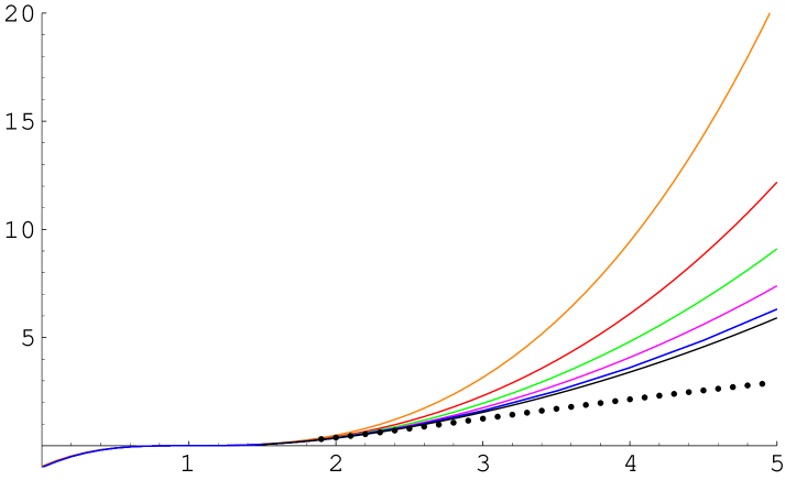
Figure 1: This figure shows the plot of the function $a^{3}f(a,L)$, computed at level $(L,2L)$ approximation, as a function of $a$. Starting from the topmost graph, the six continuous curves correspond to $L=2$, 4, 6, 8, 10 and 12 respectively. The lowermost dotted curve is an $L=\infty$ extrapolation of the data obtained with a fit of the form $a_{0}+a_{1}/L+a_{2}/L^{2}+a_{3}/L^{3}$.

If we go back to the analog of the $\widetilde{\Psi}$ variables by defining

$$\Psi=(\kappa_{0}(a)g_{o}^{2})^{-1/3}\widetilde{\Psi}$$ (5.6)

then the action takes the form:

$$S_{a}=-{1\over g_{o}^{2}}\,\Bigl{[}{1\over 2}\langle\widetilde{\Psi},\,\widetilde{\cal Q}_{a}\widetilde{\Psi}\rangle+{1\over 3}\langle\widetilde{\Psi},\,\widetilde{\Psi}*\widetilde{\Psi}\rangle\Bigr{]}\,,$$ (5.7)

where

$$\displaystyle\widetilde{\cal Q}_{a} = (g_{o}^{2}\kappa_{0}(a))^{1/3}(c_{0}+a^{-1}c_{0}L_{0})=\bigg{(}{g_{o}^{2}{\cal T}_{25}\over F(a)}\bigg{)}^{1/3}c_{0}+\bigg{(}{g_{o}^{2}{\cal T}_{25}\over a^{3}F(a)}\bigg{)}^{1/3}c_{0}L_{0}\,.$$

The data in Fig.1 suggests that $a^{3}F(a)$ grows linearly, i.e. $F(a)\sim 1/a^{2}$ for large $a$. Hence, in the $a\to\infty$ limit, the coefficient of $c_{0}$ diverges, and that of $c_{0}L_{0}$ vanishes.

$U(a,L)$	$L=4$	$L=6$	$L=8$	$L=10$	$L=12$	$L=\infty$
$a=2.0$	-.0812	-.0834	-.0846	-.0855	-.0861	-0.0904
$a=2.5$	-.1121	-.1164	-.1191	-.1210	-.1224	-0.1315
$a=3.0$	-.1372	-.1436	-.1478	-.1508	-.1530	-0.1673
$a=3.5$	-.1576	-.1660	-.1715	-.1754	-.1785	-0.1994
$a=4.0$	-.1744	-.1845	-.1911	-.1959	-.1996	-0.2251
$a=4.5$	-.1884	-.1999	-.2075	-.2130	-.2173	-0.2468
$a=5.0$	-.2002	-.2130	-.2214	-.2275	-.2323	-0.2656

Table 3: Sample numerical results for the coefficient $U(a,L)$ at different level approximation $(L,2L)$ for different values of $a$.

$V(a,L)$	$L=4$	$L=6$	$L=8$	$L=10$	$L=12$	$L=\infty$
$a=2.0$	-.1440	-.1440	-.1438	-.1436	-.1435	-0.1429
$a=2.5$	-.1884	-.1887	-.1886	-.1885	-.1884	-0.1878
$a=3.0$	-.2225	-.2232	-.2234	-.2234	-.2234	-0.2227
$a=3.5$	-.2495	-.2506	-.2510	-.2512	-.2513	-0.2515
$a=4.0$	-.2712	-.2728	-.2735	-.2738	-.2740	-0.2742
$a=4.5$	-.2892	-.2912	-.2920	-.2925	-.2928	-0.2946
$a=5.0$	-.3043	-.3066	-.3076	-.3082	-.3086	-0.3109

Table 4: Sample numerical results for the coefficient $V(a,L)$ at different level approximation $(L,2L)$ for different values of $a$. The last column of tables 3 and 4 shows a large $L$ extrapolation obtained with a fit $c_{0}+c_{1}/L+c_{2}/L^{2}+c_{3}/L^{3}$. The further large $a$ extrapolation in (5.2) is done with a more complete set of data than shown in these tables (all values of $a$ from 2 to 5 with an increment of 0.1).

We now examine the form of the D-25 brane solution. The solutions $\Psi_{L}^{a}$ are string fields belonging to the universal ghost number one subspace [3, 21] obtained by acting on the vacuum with ghost oscillators and matter Virasoro generators. Up to level 4,

$$\displaystyle\Psi_{a}^{L}= T(a,L)\Big{[} c_{1}|0\rangle+U(a,L)L^{m}_{-2}c_{1}|0\rangle+V(a,L)c_{-1}|0\rangle$$

$$\hskip-30.0pt+A(a,L)L^{m}_{-4}c_{1}|0\rangle+B(a,L)(L^{m}_{-2})^{2}c_{1}|0\rangle+C(a,L)L_{-2}^{m}c_{-1}|0\rangle+$$

$$\hskip-30.0ptD(a,L)(-3\,c_{-3}+b_{-3}c_{-1}c_{1})|0\rangle+E(a,L)b_{-2}c_{-2}c_{1}|0\rangle+\ldots\Big{]}\,.$$

Our regulation prescription instructs us to first take the large $L$ limit of $\Psi_{a}^{L}$, and then remove the regulator by sending $a\to\infty$. As shown in tables 3 and 4, up to the overall normalization $T(a,L)$ which has been factored out, the coefficients of the solution for a given regulator $a$ are fairly stable as the level is increased. Considering data for $2\leq a\leq 5$, and $L=2,4,6,8,10,12$, we first perform a large $L$ extrapolation with a fitting function of the form $c_{0}+c_{1}/L+c_{2}/L^{2}+c_{3}/L^{3}$; then we extrapolate to $a=\infty$ with a fit $\gamma_{0}+\gamma_{1}/a+\gamma_{2}/a^{2}+\gamma_{3}/a^{3}$. This procedure gives

$$\displaystyle\lim_{a\to\infty}\lim_{L\to\infty}\frac{\Psi_{a}^{L}}{T(a,L)} \cong c_{1}|0\rangle-0.4564\,L^{m}_{-2}c_{1}|0\rangle-0.4901\,c_{-1}|0\rangle$$

$$\hskip-25.0pt+\,0.0041\,L^{m}_{-4}c_{1}|0\rangle+0.0917\,(L^{m}_{-2})^{2}c_{1}|0\rangle+0.2037\,L^{m}_{-2}c_{-1}|0\rangle$$

$$\hskip-25.0pt-0.1131(-3c_{-3}+b_{-3}c_{-1})|0\rangle-0.0024\,b_{-2}c_{-2}c_{1}|0\rangle+\ldots$$

While this double extrapolation procedure is the correct general prescription, we would like to show that for certain purposes it is possible to work in the non-regulated theory, or in other words to commute the limits in (5.2) by first removing the regulator sending $a\to\infty$ and then performing level truncation in the theory with ${\cal Q}=(c(i)-c(-i))/(2i)$. In fact, we know that the non-regulated theory gives correct results about existence of classical D-$p$ brane solutions and the ratios of their tensions [5, 7] so it should be the case that the limits in (5.2) can be commuted for this class of physical questions. This will obviously be the case if we can show that up to an overall normalization, classical solutions are the same regardless of the order of limits,

$$\lim_{a\to\infty}\lim_{L\to\infty}\frac{\Psi_{a}^{L}}{T(a,L)}=\lim_{L\to\infty}\lim_{a\to\infty}\frac{\Psi_{a}^{L}}{T(a,L)}\,.$$ (5.11)

It is easy to perform numerical analysis directly at $a=\infty$ for a given level of approximation. Although the energy, being proportional to $F(a)$, goes to zero in this limit unless we compensate for it by making $\kappa_{0}(a)$ large, the solution approaches a finite limit up to the overall normalization. Numerical results are shown in table 5.

We find:

$$\displaystyle\lim_{a\to\infty}\lim_{L\to\infty}\frac{\Psi_{a}^{L}}{T(a,L)} \cong c_{1}|0\rangle-0.4603\,L^{m}_{-2}c_{1}|0\rangle-0.4900\,c_{-1}|0\rangle$$

$$\hskip-35.0pt+\,0.0029\,L^{m}_{-4}c_{1}|0\rangle+0.1049\,(L^{m}_{-2})^{2}c_{1}|0\rangle+0.2311\,L^{m}_{-2}c_{-1}|0\rangle$$

$$\hskip-35.0pt-0.1258(-3c_{-3}+b_{-3}c_{-1})|0\rangle+0.0001\,b_{-2}c_{-2}c_{1}|0\rangle+\ldots$$

This is compatible with (5.2) and (5.11).

We thus find evidence that classical solutions of VSFT are independent of the order of limits, up to an overall normalization factor that needs to be adjusted so as to keep the tension fixed. This justifies the analytic treatment of the equations of motion based on matter/ghost factorization, which has been an important assumption in all studies of VSFT, and which holds only in the $a\to\infty$ limit. Moreover, we can study numerically the D-25 brane solution in the $a\to\infty$ theory at fixed $L$, which is much simpler than taking the $L\to\infty$ limit first and then taking the $a\to\infty$ limit.

	$U(L)$	$V(L)$	$A(L)$	$B(L)$	$C(L)$	$D(L)$	$E(L)$
$L=2$	-.2879	-.4576	–	–	–	–	–
$L=4$	-.3015	-.4357	.0094	.0358	.1082	-.0844	-.0103
$L=6$	-.3394	-.4596	.0080	.0523	.1440	-.0995	-.0037
$L=8$	-.3631	-.4708	.0072	.0627	.1640	-.1072	-.0019
$L=10$	-.3798	-.4771	.0066	.0700	.1768	-.1114	-.0011
$L=12$	-.3923	-.4811	.0060	.0755	.1858	-.1141	-.0007
$L=\infty$	-.4603	-.4900	.0029	.1049	.2311	-.1258	.0001

Table 5: Coefficients of the $a=\infty$ solution, at different level approximation $(L,2L)$ (we use $U(\infty,L)\equiv U(L)$, and he same convention for the other coefficients). The last row shows an extrapolation to infinite level with a fitting function of the form $a_{0}+a_{1}/L+a_{2}/L^{2}+a_{3}/L^{3}$.

	$v_{2}$	$\widetilde{v}_{2}$	$v_{4}$	$\widetilde{v}_{4}$	$v_{6}$
$L=2$	-.2879	-.4576	–	–	–
$L=4$	-.3364	-.4736	.0056	-.00193	–
$L=6$	-.3655	-.4816	.0048	-.00216	-.00111
$L=8$	-.3852	-.4861	.0043	-.00197	-.00080
$L=10$	-.3999	-.4891	.0039	-.00176	-.00065
$L=12$	-.4105	-.4912	.0036	-.00157	-.00056
$L=\infty$	-.4778	-.5027	.0012	-.00007	-.0002

Table 6: Coefficients of the $a=\infty$ solution written as an exponential of matter and twisted ghost Virasoro operators, at different level approximation $(L,3L)$. The last row shows an extrapolation to infinite level with a fitting function of the form $a_{0}+a_{1}/L+a_{2}/L^{2}+a_{3}/L^{3}$.

It is illuminating to write the D-25 brane solution in a basis of Fock states obtained by acting on the zero-momentum tachyon with the matter Virasoro generators $L^{m}_{-n}$ and the ghost Virasoro generators $L^{{}^{\prime}g}_{-n}$ ($n\geq 2$) of the twisted $bc$ system introduced in section 4. It turns out that to a very good degree of accuracy the solution can be written as

$$\Psi_{a=\infty}\sim\exp(\sum_{n=1}^{\infty}v_{2n}L^{m}_{-2n})\exp(\sum_{n=1}^{\infty}\widetilde{v}_{2n}L^{{}^{\prime}g}_{-2n})c_{1}|0\rangle.$$ (5.13)

This is precisely the form expected for a surface state of the twisted BCFT introduced in section 4. The results for the coefficients $v_{2n}$ and $\widetilde{v}_{2n}$ at various level approximations $(L,3L)$ are shown in table 6. Extrapolating for $L\to\infty$ with a fit of the form $a_{0}+a_{1}/L+a_{2}/L^{2}+a_{3}/L^{3}$ we find

$$\displaystyle\Psi_{a=\infty} \sim \exp(-0.5027L^{{}^{\prime}g}_{-2}-0.00007L^{{}^{\prime}g}_{-4}+\dots)c_{1}|0\rangle_{g}$$

$$\otimes\exp(-0.4778L^{m}_{-2}+0.0012L^{m}_{-4}-0.0002L^{m}_{-6}+\dots)|0\rangle_{m}\,.$$

We note that although the solution has precisely the form expected for a surface state of the auxiliary matter-ghost system, it does not approach the twisted sliver $\Xi^{\prime}$, for which the coefficient of $L^{\prime}_{-2}$ is $-1/3$. This should not bother us, however, since we can generate many other surface states (related to the sliver by a singular or non-singular reparametrization of the string coordinate symmetric about the mid-point) which are all projectors. Moreover, at least formally, all rank one projectors are gauge-related in VSFT. The numerical result (5.2) strongly suggests that as $L\to\infty$ the solution is in fact approaching the remarkably simple state

$$|B^{\prime}\rangle\sim\exp(-\frac{1}{2}(L^{m}_{-2}+L^{{}^{\prime}g}_{-2})c_{1}|0\rangle,$$ (5.15)

which we call the (twisted) butterfly state. It is possible to show that the state $|B^{\prime}\rangle$ is indeed a projector of the $*^{\prime}$ algebra and an exact solution of the VSFT equations. In the next section we shall come back to this point.

Let us finally check numerically that the Siegel gauge D-25 brane solution obtained in level truncation solves the equation of motion of VSFT with our proposed ${\cal Q}$. To this end we take the solution $\Psi_{a=\infty}$ compute $\Psi_{a=\infty}*\Psi_{a=\infty}$, and try to determine ${\cal Q}=(c_{0}+\sum_{n\geq 1}u_{2n}(c_{2n}+c_{-2n}))$ up to a constant of proportionality using the equation:

$$\Psi_{a=\infty}*\Psi_{a=\infty}\propto{\cal Q}\Psi_{a=\infty}\,.$$ (5.16)

The results for the coefficients $u_{2n}$ at various level approximation $(L,3L)$ are shown in table 7 and are indeed consistent with our choice (2.5) for ${\cal Q}$.

	$u_{2}$	$u_{4}$	$u_{6}$	$u_{8}$	$u_{10}$
$L=2$	-.8020	–	–	–	–
$L=4$	-.8672	.7249	–	–	–
$L=6$	-.9003	.7918	-.6854	–	–
$L=8$	-.9201	.8333	-.7451	.6615	–
$L=10$	-.9334	.8627	-.7868	.7138	-.6457
$L=\infty$	-.9969	.9983	-.923	–	–

Table 7: Coefficients of the BRST operator deduced from the $a=\infty$ solution, at different level approximations $(L,3L)$.The last row shows an extrapolation to infinite level with fits of the form $a_{0}+a_{1}/L+a_{2}/L^{2}+a_{3}/L^{3}$ ($a_{3}\equiv 0$ for $u_{4}$, $a_{3}=a_{2}\equiv 0$ for $u_{6}$).

6 The Butterfly State

The level truncation results have led to the discovery of a new simple projector, the butterfly state, different from the sliver. There are in fact several surface states that can be written in closed form and shown to be projectors using a variety of analytic approaches. In this section we briefly state without proof some of the relevant results. A thorough discussion will appear in a separate publication [26].

Consider the class of surface states $|B_{\alpha}\rangle$, defined through:

$$\langle B_{\alpha}|\phi\rangle\equiv\langle f_{\alpha}\circ\phi(0)\rangle_{D}$$ (6.1)

with

$$f_{\alpha}(\xi)={1\over\alpha}\sin(\alpha\tan^{-1}\xi)\,.$$ (6.2)

As $\alpha\to 0$, we recover the sliver. For $\alpha=1$ we have the butterfly state $|B\rangle\equiv|B_{\alpha=1}\rangle$, defined by the map

$$f_{1}(\xi)=\frac{\xi}{\sqrt{1+\xi^{2}}}\,.$$ (6.3)

In operator form the butterfly can be written as

$$|B\rangle=\exp(-\frac{1}{2}L_{-2})|0\rangle\,.$$ (6.4)

For any $\alpha$, these states can be shown to be idempotents of the $*$ algebra,

$$|B_{\alpha}\rangle*|B_{\alpha}\rangle=|B_{\alpha}\rangle\,.$$ (6.5)

Moreover, in analogy with the sliver, the wave-functional of $|B_{\alpha}\rangle$ factorizes into a product of a functional of the left-half of the string and another functional of the right half of the string. These states are thus naturally thought as rank-one projectors in the half-string formalism [6, 9, 10]. The key property that ensures factorization is the singularity of the conformal maps at the string midpoint,

$$f_{\alpha}(\pm i)=\pm i\infty\,.$$ (6.6)

It is possible to give a general argument [26] that all sufficiently well-behaved conformal maps with this property give rise to split wave-functionals.

The case $\alpha=1$ is special because the wave-functional of the butterfly $|B_{\alpha=1}\rangle$ factors into the product of the vacuum wave-functional of the right half-string and the vacuum wave-functional of the left half-string. It is thus in a sense the simplest possible projector. It is quite remarkable that the same state emerges in VSFT as the numerical solution preferred by the level truncation scheme.

Finally, in complete analogy with the ‘twisted’ sliver $\Xi^{\prime}$, the ‘twisted’ states $|B^{\prime}_{\alpha}\rangle$ solve the VSFT equations of motion with ${\cal Q}=(c(i)-c(-i))/(2i)$,

$${\cal Q}|B^{\prime}_{\alpha}\rangle\propto|B^{\prime}_{\alpha}\rangle*|B^{\prime}_{\alpha}\rangle\,.$$ (6.7)

Indeed the proof of section 4 that $\Xi^{\prime}$ satisfies the VSFT equations of motion ${\cal Q}\Xi^{\prime}\propto\Xi^{\prime}*\Xi^{\prime}$ only depends on the fact that the map $f(\xi)=\tan^{-1}\xi$ associated with the sliver takes the points $\pm i$ to $\pm i\infty$. As can be seen from (6.6), this property is shared by the map $f_{\alpha}$ associated with the state $|B_{\alpha}\rangle$.

7 Gauge invariant operators in OSFT and VSFT

Since open string field theory on an unstable D-brane has no physical excitations at the tachyon vacuum, the only possible observables in this theory are correlation functions of gauge invariant operators. A natural set of gauge invariant operators in this theory has been constructed in [28] by using the open/closed string vertex that emerges from the studies of [27]. In this section we will describe in detail these gauge invariant operators in OSFT and show how they give rise to gauge invariant operators in VSFT. It would be interesting to analyze the correlation functions of these operators around the tachyon vacuum by using OSFT in the level truncation scheme.

The same gauge invariant operators discussed here have been considered independently by Hashimoto and Itzhaki, who examined the gauge invariance in an explicit oscillator construction, and motivated their role mostly in the context of OSFT [39].

We shall begin by reviewing the construction of ref.[28] and then we will consider the generalization to VSFT.

7.1 Gauge invariant operators in OSFT

The original cubic open string field theory [1] describing the dynamics of the unstable D-brane, is described by the action:

$$S=-{1\over g_{o}^{2}}\,\Big{[}{1\over 2}\langle\Phi,Q_{B}\Phi\rangle+{1\over 3}\langle\Phi,\Phi*\Phi\rangle\Big{]}\,,$$ (7.1)

with gauge invariance:

$$\delta|\Phi\rangle=Q_{B}|\Lambda\rangle+|\Phi*\Lambda\rangle-|\Lambda*\Phi\rangle\,.$$ (7.2)

Here $Q_{B}$ is the BRST charge, $g_{o}$ is the open string coupling constant, $|\Phi\rangle$ is the string field, and $|\Lambda\rangle$ is the gauge transformation parameter. In this theory there are gauge invariant operators ${\cal O}_{V}(\Phi)$ corresponding to every on-shell closed string state represented by the BRST invariant, dimension $(0,0)$ vertex operator $V=c\bar{c}V_{m}$, where $V_{m}$ is a dimension (1,1) primary in the bulk matter CFT. Given any such closed string vertex operator $V$, we define ${\cal O}_{V}(\Phi)$ as the following linear function of the open string field $\Phi$:

$${\cal O}_{V}(\Phi)\equiv\langle h_{1}\circ(V(i)\Phi(0))\rangle_{D}=\langle V(0)h_{1}\circ\Phi(0)\rangle_{D}\,,$$ (7.3)

where $h_{N}$ has been defined in eq.(2.21), and $\langle~{}\rangle_{D}$ denotes correlation function on a unit disk. Since $V$ is dimension $(0,0)$ it is not affected by the conformal map $h_{1}$ despite being located at the singular point $z=i$. In [28] these operators were added to the OSFT action and it was shown that the resulting Feynman rules would generate a cover of the moduli spaces of closed Riemann surfaces with boundaries and closed string punctures thus producing the appropriate closed string amplitudes. The operators ${\cal O}_{V}(\Phi)$ can be interpreted as the open string one point function

$${\cal O}_{V}(\Phi)=\langle{\cal I}|V(i)|\Phi\rangle\,,$$ (7.4)

where $\langle{\cal I}|$ is the identity state of the $*$-product. The world sheet picture is clear, ${\cal O}_{V}(\Phi)$ corresponds to the amputated version of a semi-infinite strip whose edge represents an open string, the two halves of which are glued and a closed string vertex operator is located at the conical singularity. Gauge invariance of ${\cal O}_{V}(\Phi)$ under (7.2) follows from the BRST invariance of $V$ and the relations

$$|A\rangle*(V(i)|B\rangle)=V(i)|A*B\rangle,\qquad(V(i)|A\rangle)*|B\rangle=V(i)|A*B\rangle\,.$$ (7.5)

7.2 Gauge invariant operators in VSFT

Since the VSFT field $\Psi$ must be related to the original unstable D-brane OSFT field $|\Phi\rangle$ by a field redefinition, the existence of gauge invariant observables in the OSFT implies that there must exist such quantities in the VSFT as well. Even though the explicit relation between $|\Psi\rangle$ and $|\Phi\rangle$ is not yet known, we now argue that the VSFT gauge invariant observables actually take the same form as in OSFT.

The possible field redefinitions relating VSFT and OSFT were discussed in ref.[4]. If we denote by $|\Phi_{0}\rangle$ the classical OSFT solution describing the tachyon vacuum, then the shifted string field $|\widetilde{\Phi}\rangle=|\Phi\rangle-|\Phi_{0}\rangle$ may be related to $|\Psi\rangle$ by homogeneous redefinitions preserving the structure of the cubic vertex, namely

$$(g_{o}^{2}\kappa_{0})^{1/3}\,|\Psi\rangle=e^{-K}|\widetilde{\Phi}\rangle\,,$$ (7.6)

where $K$ satisfies:

$$\displaystyle K(A*B) = (KA)*B+A*(KB)\,,$$

$$\langle KA,B\rangle = -\langle A,KB\rangle\,.$$ (7.7)

The explicit normalization factor $(g_{o}^{2}\kappa_{0})^{1/3}$ on the left hand side of eq.(7.6) has been chosen to ensure the matching of the cubic terms in (2.1) and (7.1) (see eq.(2.10)). Two general class of examples of $K$ satisfying (7.2) are:

$$K|A\rangle=\sum_{n}a_{n}K_{n}|A\rangle\,,$$ (7.8)

where $K_{n}=L_{n}-(-1)^{n}L_{-n}$, and

$$K|A\rangle=|S*A\rangle-|A*S\rangle\,,$$ (7.9)

for some ghost number zero state $|S\rangle$. Let us now consider the gauge invariant operator

$${\cal O}_{V}(\widetilde{\Phi})=\langle V(0)h_{1}\circ\widetilde{\Phi}(0))\rangle_{D}=\langle{\cal I}|V(i)|\widetilde{\Phi}\rangle\,,$$ (7.10)

invariant under the gauge transformation

$$\delta|\widetilde{\Phi}\rangle=Q_{B}|\Lambda\rangle+|(\widetilde{\Phi}+\Phi_{0})*\Lambda\rangle-|\Lambda*(\widetilde{\Phi}+\Phi_{0})\rangle\,,$$ (7.11)

and study what happens to this under an infinitesimal field redefinition generated by a $K$ of the form (7.8) or (7.9). It is easy to see that both these field redefinitions preserve the form of ${\cal O}_{V}$, replacing $\widetilde{\Phi}$ by $(g_{o}^{2}\kappa_{0})^{1/3}\Psi$. For transformations of the form (7.8) this follows because $V(i)$, being a dimension zero primary, commutes with the $K_{n}$’s and the identity is annihilated by $K_{n}$. For transformations of the form (7.9), form invariance follows from eq.(7.5). Thus if $\widetilde{\Phi}$ and $\Psi$ are related by a field redefinition of the form (7.6), with $K$ being a combination of transformations of the type (7.8) or (7.9), then we can conclude that ${\cal O}_{V}(\widetilde{\Phi})$ is given by $(g_{o}^{2}\kappa_{0})^{1/3}{\cal O}_{V}(\Psi)$, with

$${\cal O}_{V}(\Psi)=\langle V(0)h_{1}\circ\Psi(0))\rangle_{D}=\langle{\cal I}|V(i)|\Psi\rangle\,.$$ (7.12)

This must be a gauge invariant operator in VSFT. Invariance of (7.12) under the VSFT gauge transformation (2.7) follows directly from (7.5), and the relation $\langle{\cal I}|A*B\rangle=\langle A|B\rangle$. Invariance under (2.6) requires

$$\langle{\cal I}|V(i){\cal Q}|\Lambda\rangle\equiv\langle h_{1}\circ(V(i){\cal Q}\Lambda(0))\rangle_{D}=0\,.$$ (7.13)

If we choose ${\cal Q}$ to be of the form $\sum_{n}u_{n}{\cal C}_{n}$, then for any choice of the coefficients $u_{n}$, ${\cal Q}$ commutes with $V(i)$. Thus if we further restrict the $u_{n}$’s so that ${\cal Q}$ annihilates $|{\cal I}\rangle$, then the gauge invariance of ${\cal O}_{V}$ is manifest. Our choice ${\cal Q}=(c(i)-c(-i))/2i$, however, does not annihilate $|{\cal I}\rangle$ unless we define ${\cal Q}$ in a specific manner discussed in (2.24). Nevertheless, as we shall now show, ${\cal Q}$ annihilates $V(i)|{\cal I}\rangle$ independently of the definition (2.24) and simply because of the collision of local ghost insertions. Consider a definition of ${\cal Q}$ that does not annihilate $|{\cal I}\rangle$, by putting the operators in ${\cal Q}$ at $i+\epsilon$ for some finite $\epsilon$ and then take the $\epsilon\to 0$ limit. This gives:

$$\langle h_{1}\circ(V(i){\cal Q}\Lambda(0))\rangle_{D}\propto\lim_{\epsilon\to 0}\,\Bigl{\langle}h_{1}\circ\Big{(}V(i)(c(i+\epsilon)-\bar{c}(i+\epsilon))\Lambda(0)\Big{)}\Bigr{\rangle}_{D}$$ (7.14)

$$= \lim_{\epsilon\to 0}\,\Bigl{\langle}V(h_{1}(i))\Bigl{\{}{c(h_{1}(i+\epsilon))\over h_{1}^{\prime}(i+\epsilon)}-{\bar{c}(h_{1}(i+\epsilon))\over\bar{h}_{1}^{\prime}(i+\epsilon))}\Bigr{\}}\,h_{1}\circ\Lambda(0)\Bigr{\rangle}_{D}\,.$$

Using the results:

$$h_{1}(i+\epsilon)\sim\epsilon^{2},\quad h_{1}^{\prime}(i+\epsilon)\sim\epsilon,\quad V(0)c(\eta)\sim\eta,\qquad V(0)\bar{c}(\eta)\sim\eta\,,$$ (7.15)

we see that the expression between $\Bigl{\langle}\cdots\Bigr{\rangle}$ vanishes linearly in $\epsilon$. Thus ${\cal O}_{V}(\Psi)$ defined in (7.12) is invariant under each of the transformations (2.6) and (2.7) for ${\cal Q}$ given in (2.5).

It is interesting to relate the present discussion to our observations on the cohomology of ${\cal Q}$ below equation (2.5). It was noted there that ${\cal Q}$ closed states had to have ghost insertions at the open string midpoint. The question that emerges is whether or not the gauge invariant operators discussed here are ${\cal Q}$ trivial. Presumably they are not. Indeed, thinking of $c\bar{c}V_{m}$ as $c$ acting on $\bar{c}V_{m}$ we find that the insertion of $\bar{c}V_{m}$, which is not of dimension zero but rather of negative dimension, on a point with a defect angle leads to a divergence. Therefore one cannot think of the gauge invariant operators as ordinary trivial states. Alternatively, one may wonder if the condition that the closed string vertex operator $V$ be a dimension-zero primary can be relaxed and still have ${\cal O}_{V}$ be a sensible gauge invariant operator. Again, the answer is expected to be no. Inserting an operator with dimension different from zero at the conical singular point either gives zero or infinity. Moreover, if the operator is not primary there are also difficulties with equation (7.5).

7.3 Classical expectation value of ${\cal O}_{V}$

Given a classical solution of VSFT representing a D-brane we can ask what is the value of

$${\cal O}_{V}(\Psi_{cl})=\langle{\cal I}|V(i)|\Psi_{cl}\rangle\,.$$ (7.16)

For $|\Psi_{cl}\rangle=|\Psi_{g}\rangle\otimes|\Psi_{m}\rangle$, and $V=c\bar{c}V_{m}$, we have:

$${\cal O}_{V}(\Psi_{cl})=\langle{\cal I}_{g}|c\bar{c}(i)|\Psi_{g}\rangle\,\langle{\cal I}_{m}|V_{m}(i)|\Psi_{m}\rangle\,.$$ (7.17)

The ghost factor is universal, $-$ common to all D-brane solutions, and all closed string vertex operators of the form $c\bar{c}V_{m}$. If we take $|\Psi_{m}\rangle$ to be a solution of the form discussed in [8], representing a D-brane associated with some boundary CFT $\widetilde{BCFT}$, then it is easy to show following the techniques of [8] that $\langle{\cal I}_{m}|V(i)|\Psi_{m}\rangle$ has the interpretation of a one point correlation function on the disk, with closed string vertex opertor $V_{m}$ inserted at the center of the disk, and the boundary condition associated with $\widetilde{BCFT}$ on the boundary of the disk. This, in turn can be interpreted as $\langle\widetilde{B}_{m}|V_{m}\rangle$ where $\langle\widetilde{B}_{m}|$ is the matter part of the boundary state associated with $\widetilde{BCFT}$ and $|V_{m}\rangle$ is the closed string state created by the vertex operator $V_{m}$.

8 Closed string amplitudes in VSFT

In this section we give our proposal for the emergence of pure closed string amplitudes in the context of VSFT. The basic idea is that the open string correlation of the gauge invariant observables discussed in the previous section give rise to closed string amplitudes obtained by integration over the moduli spaces of Riemann surfaces without boundaries. In order to justify this we will have to make use of the regularized version of VSFT.

8.1 Computation of correlation functions of ${\cal O}_{V}$

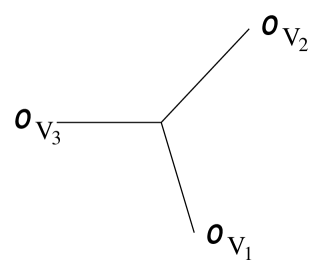
Figure 2: The feynman diagram contributing to the correlation function $\langle\langle{\cal O}_{V_{1}}{\cal O}_{V_{2}}{\cal O}_{V_{3}}\rangle\rangle$.

We shall now study correlation functions of the operators ${\cal O}_{V}$ in VSFT. In particular, we shall analyze the following gauge invariant correlation functions:

$$\lll{\cal O}_{V_{1}}(\Psi)\cdots{\cal O}_{V_{n}}(\Psi)\rangle\rangle$$ (8.18)

where $\lll~{}\rangle\rangle$ stands for correlation functions in string field theory and should not be confused with correlation functions in two dimensional conformal field theory. These correlation functions are calculated by the usual Feynman rules of string field theory, $-$ in particular for $n=3$ the tree level correlation function receives contribution from just one Feynman diagram shown in Fig.2. In computing these Feynman diagrams we shall work with the regulated action (5.1) and take the $a\to 0$ limit at the end. Including all the normalization factors, the Siegel gauge propagator is given by:

$$a(\kappa_{0}(a))^{-1}{b_{0}\over L_{0}+a}={a\over\kappa_{0}(a)}b_{0}\int_{0}^{\infty}dle^{-l(L_{0}+a)}\,.$$ (8.19)

We should, however, keep in mind that this regularization procedure is ad hoc, and so the results obtained from this should be interpreted with caution The correct regularization procedure presumably comes from replacing the singular reparametrization discussed in section 2.2 by a nearly singular reparametrization.

Since the propagator (8.19) is closely related to the propagator of OSFT, and reduces to it up to an overall normalization in the $a\to 0$ limit, it will be useful to first review the calculation of these correlation function in OSFT around the D-25-brane background. In OSFT, the Feynman diagrams just have closed string vertex operators attached to strips of length $\ell_{i}$ and these strips, together with internal open string propagators, are glued with three open string vertices. So a typical diagram will have schematically

$$\prod_{i}\int_{0}^{\infty}d\ell_{i}e^{-\ell_{i}L_{0}}\prod_{J}\int_{0}^{\infty}d\ell_{J}e^{-\ell_{J}L_{0}}$$

where the $\ell_{J}$ are intermediate propagator lengths. For an amplitude with $n$ external closed strings there are altogether $(2n-3)$ propagators and $(n-2)$ vertices. Let us denote by $l_{\alpha}$ ($1\leq\alpha\leq(2n-3)$) the lengths of the strips associated with these $(2n-3)$ propagators. Thus the contribution to the amplitude can be written as (ignoring powers of the open string coupling constant $g_{o}$):

$$\int\prod_{\alpha=1}^{2n-3}dl_{\alpha}F(l_{1},\ldots l_{2n-3})$$ (8.20)

for some appropriate integrand $F$ which is computed in terms of correlators of closed string vertex operators and ghost factors associated with the propagators on an appropriate Riemann surface.

If we repeat the calculation in VSFT with the regularized propagator (8.19), we get an additional factor $e^{-a\sum l_{\alpha}}$ in the integrand. This, in effect will restrict the integration region to $l_{\alpha}$ of order $a^{-1}$ or less. Also each propagator carries a multiplicative factor of $a/\kappa_{0}(a)$ and each vertex carries a multiplicative factor of $\kappa_{0}(a)$. Thus the amplitude now takes the form:

$$\displaystyle A_{n} = (a/\kappa_{0}(a))^{2n-3}(\kappa_{0}(a))^{n-2}\int\prod_{\alpha=1}^{2n-3}dl_{\alpha}e^{-a\sum l_{\alpha}}F(l_{1},\ldots l_{2n-3})$$

$$= \hskip-10.0pt(a^{2}/\kappa_{0}(a))^{n}a^{-3}\kappa_{0}(a)\int_{0}^{\infty}\hskip-10.0ptdv\int\prod_{\alpha=1}^{2n-3}dl_{\alpha}\delta(v-\sum l_{\alpha})e^{-av}F(l_{1},\ldots l_{2n-3})\,.$$

We can absorb the $n$ factors of $(a^{2}/\kappa_{0}(a))$ into a multiplicative renormalization of the operators ${\cal O}_{V}$. Using eq.(5.4) with ${\cal E}_{a}={\cal T}_{25}$, the renormalized amplitude may be written as:

$$A_{n}={{\cal T}_{25}\over a^{3}F(a)}\int_{0}^{\infty}dv\,e^{-av}\,\int\prod_{\alpha=1}^{2n-3}dl_{\alpha}\,\delta(v-\sum l_{\alpha})F\Big{(}l_{1},\ldots l_{2n-3}\Big{)}\,.$$ (8.22)

Figure 3: The Riemann surface representations of the Feynman diagram contribution to the three closed string amplitude. $V_{i}$ denote the locations of the closed string vertex operators, $l_{\alpha}$ denote the lengths of the strips representing open string propagators, and AMB, BMC and CMA denote the three strings interacting via the three string vertex with a common mid-point $M$. The thick line at the bottom is the boundary of the world-sheet diagram created from the Feynman diagram. The two diagrams originate from two different contributions to the three string vertex, corresponding to $\langle A,\,B*C\rangle$ and $\langle A,\,C*B\rangle$ respectively.

$F(l_{1},\ldots l_{2n-3})$ is computed by evaluating a correlation function on a Riemann surface of the form shown in Fig.3. Since $v$ in the above integral represents the sum of the length parameters $l_{\alpha}$, we have $l_{\alpha}\leq v$, and the closed string vertex operators are inserted within a distance of order $v$ of each other. The boundary, shown by the thick line at the bottom, has length $2v$ since each length parameter $l_{\alpha}$ contributes a length $2l_{\alpha}$ to the boundary. Finally, the height of the diagram, measured by the distance between the boundary and the closed string vertex operators, is constant and equal to $\pi/2$ – this is because open string strips have width $\pi$. In addition to the closed string vertex operators, the correlator also includes an insertion of $b_{0}$ on each propagator.

Let us now rescale the metric on this world-sheet by multiplying all lengths by $\pi v^{-1}$. In the resulting metric, and with $v$ now small, the Riemann surface looks like a long cigar of circumference $2\pi$ and height $l_{c}=\pi^{2}/(2v)$. All the closed string vertex operators are inserted within a finite distance of each other at the closed end of the cigar, and their positions are naturally parametrized by quantities $u_{\alpha}$ defined, for $\alpha=1,2\cdots,2n-3$, as

$$u_{\alpha}=2\pi\,{l_{\alpha}\over v}\quad\to\quad\sum_{\alpha}u_{\alpha}=2\pi\,.$$ (8.23)

The other end of the cigar is open and represents the boundary of the surface. The integration contours for the $b$-integrals run parallel to the length of the cigar. We will call this surface ${\cal C}_{v}(\vec{u})$, and as defined it is a cylinder of height $\pi^{2}/(2v)$, circumference $2\pi$, with one end open and the other sealed and having closed string punctures with positions parameterized by the $u_{\alpha}$. We can use $v$ and $u_{\alpha}$ as independent variables of integration. Since the $b$-contour integrals in the correlation function guarantee that the integrand transforms as a volume form $dv\wedge du_{1}\wedge\cdots$ in the moduli space, we can formally denote these insertions as $B_{v}B_{\vec{u}}$, where $B_{v}$ denotes a single $b$ insertion associated with the $v$-integration and $B_{\vec{u}}$ is product of $(2n-4)$ $b$-insertions associated with the integration over $\vec{u}$. Calling ${\cal M}(\vec{u})$ the moduli space of $u_{\alpha}$’s, the amplitude in (8.22) can thus be written as

$$A_{n}={{\cal T}_{25}\over a^{3}F(a)}\int_{0}^{\infty}dv\,e^{-av}\,\int_{{\cal M}(\vec{u})}\langle V_{1}\cdots V_{n}B_{v}B_{\vec{u}}\rangle_{{\cal C}_{v}(\vec{u})}\,.$$ (8.24)

Figure 4: Pictorial representation of ${\cal C}_{0}(\vec{u})$ and ${\cal V}_{b}$ which are glued together to produce the surface ${\cal C}_{v}(\vec{u})$.

In order to proceed further we build the surface ${\cal C}_{v}(\vec{u})$ by sewing the semi-infinite cylinder ${\cal C}_{0}(\vec{u})$, obtained when $v=0$, to the closed/boundary vertex ${\cal V}_{b}$ represented by a semi-infinite cylinder of circumference $2\pi$ ending on an open boundary. If we denote by $w_{1}$ and $w_{2}$ the coordinates used to describe the above two cylinders ${\cal C}_{v}(\vec{u})$ and ${\cal V}_{b}$, with $w_{i}\equiv w_{i}+2\pi$ and $\Im(w_{i})<0$, and we let $z_{i}=\exp(-iw_{i})$; the sewing relation $z_{1}z_{2}=t$, with real $t$ produces the surface ${\cal C}_{v}$ with $v=-\pi^{2}/(2\ln t)$. We therefore have that the amplitude in question can be written as:

$$\displaystyle A_{n} = {{\cal T}_{25}\over a^{3}F(a)}\int_{0}^{\infty}dv\,e^{-av}\,\int_{{\cal M}(\vec{u})}\sum_{k}\langle V_{1}\cdots V_{n}B_{\vec{u}}\chi_{k}\rangle_{{\cal C}_{0}(\vec{u})}$$ (8.25)

$$\qquad\qquad\qquad\qquad\qquad\quad\cdot\,\,\langle\chi_{k}^{c}|B_{v}e^{-{\pi^{2}\over 2v}(L_{0}+\bar{L}_{0})}|{\cal V}_{b}\rangle\,,$$

where the $\chi_{k}$ is a basis element in the space of ghost number two closed string vertex operators, $\chi_{k}^{c}$ is the conjugate basis of ghost number four vertex operators satisfying $\langle\chi_{k}^{c}|\chi_{l}\rangle=\delta_{kl}$, $|{\cal V}_{b}\rangle$ denotes the boundary state associated with the D-brane under consideration, and $L_{0},\bar{L}_{0}$ refers to the closed string Virasoro generators. In the first correlator, ${\chi_{k}}$ is inserted on the puncture at infinity, and the second correlator is the one point function on the semi-infinite cylinder.

We now need to determine $B_{v}$. This is done by going to the $l_{c}=\pi^{2}/2v$ coordinate system, and using the transformation property of the $b$-insertions under a change of coordinates. In particular, we have

$$B_{v}dv=B_{l_{c}}dl_{c}\,.$$ (8.26)

Furthermore the form of $B_{l_{c}}$ is well known, $-$ it simply corresponds to an insertion of a contour integral of $(b+\bar{b})$ along the circumference of the cigar. We shall denote this by $(b_{0}+\bar{b}_{0})$. This gives:

$$dvB_{v}={\pi^{2}\over 2v^{2}}dv(b_{0}+\bar{b}_{0})\,.$$ (8.27)

Substituting this into eq.(8.25) we get,

$$\displaystyle A_{n} = {{\cal T}_{25}\over a^{3}F(a)}\,{\pi^{2}\over 2}\,\int_{0}^{\infty}{dv\over v^{2}}\,e^{-av}\,\int_{{\cal M}(\vec{u})}\sum_{k}\langle V_{1}\cdots V_{n}B_{\vec{u}}\chi_{k}\rangle_{{\cal C}_{0}(\vec{u})}$$ (8.28)

$$\hskip 60.0pt\cdot\,\langle\chi_{k}^{c}|(b_{0}+\bar{b}_{0})e^{-{\pi^{2}\over 2v}(L_{0}+\bar{L}_{0})}|{\cal V}_{b}\rangle\,,$$

The key geometrical insight now is that the moduli space ${\cal M}(\vec{u})$ defines a space of surfaces ${\cal C}_{0}(\vec{u})$ which is precisely the moduli space ${\cal M}_{n+1}$ of $n+1$-punctured spheres. This is a rigorous result and follows from a new minimal area problem that will be discussed in the next subsection. Therefore the integral above can be written as

$${{\cal T}_{25}\over a^{3}F(a)}\,{\pi^{2}\over 2}\,\sum_{k}\int{dv\over v^{2}}e^{-av}e^{-{\pi^{2}\over 2v}(h_{k}+\bar{h}_{k})}\langle\chi_{k}^{c}|(b_{0}+\bar{b}_{0})|{\cal V}_{b}\rangle$$ (8.29)

$$\hskip 60.0pt\cdot\,\int_{{\cal M}_{n+1}}\langle V_{1}\cdots V_{n}B_{\vec{u}}\chi_{k}\rangle_{{\cal C}_{0}(\vec{u})}$$

$$= \sum_{k}C_{k}A_{c}(V_{1},\ldots V_{n},\chi_{k})\,,$$

where $(h_{k},\bar{h}_{k})$ is the conformal weight of $\chi_{k}$, and $A_{c}(V_{1},\ldots V_{n},\chi_{k})$ is the $(n+1)$-point closed string amplitude of states $V_{1},\ldots V_{n}$ and $\chi_{k}$. $C_{k}$ are constants defined as:

$$C_{k}={{\cal T}_{25}\over a^{3}F(a)}\,{\pi^{2}\over 2}\,\int{dv\over v^{2}}e^{-av}e^{-{\pi^{2}\over 2v}(h_{k}+\bar{h}_{k})}\langle\chi_{k}^{c}|(b_{0}+\bar{b}_{0})|{\cal V}_{b}\rangle\,.$$ (8.30)

The multiplicative factor $C_{k}$ is non-zero in the $a\to 0$ limit only for $h_{k}+\bar{h}_{k}\leq 0$. For this range of values of $(h_{k},\bar{h}_{k})$ $C_{k}$’s are actually infinite due to the divergence in the $v$-integral from $v\simeq 0$ region. However, note that the multiplicative factor ${\cal T}_{25}/(a^{3}F(a))$ vanishes as $a\to\infty$ as is seen from Fig.1. Thus this competes against the divergent $v$-integral. It will be interesting to see if in the correct regularization procedure inherited from OSFT, the divergences in the $v$ integral are also regulated (as will happen, for example, if the kinetic operator is multiplied by an additional factor of $e^{\epsilon L_{0}}$ for some small $\epsilon$), and the final answer for the closed string amplitude is actually finite.

We also note that among the contributions to (LABEL:econt) is the contribution due to the zero momentum dilaton intermediate state. By the soft dilaton theorem, this is proportional to the on-shell $n$-point closed string amplitude on the sphere. One could again speculate that in the correct regularization procedure this is the only contribution that survives, and so the correlation function (8.18) in the correctly regularized VSFT actually gives us back the on-shell $n$-point amplitude at genus zero. A similar argument has been given in [38] in the context of boundary string field theory.

Since the regularization procedure we have been using is ad hoc, one can ask what aspect of our results can be trusted in a regularization independent manner. To this end, note that if the kinetic operator is simply $c_{0}$, then the corresponding propagator is represented by a strip of zero length. Thus whatever be the correct regularization procedure, the regulated propagator will be associated with strips of small lengths if the regularization parameter (analog of $a^{-1}$) is small. As our analysis shows, in this case the corresponding Feynman diagram contribution to (8.18) will be associated with a world-sheet diagram with small hole, and this, in turn, is related to genus zero correlation functions of closed string vertex operators with one additional closed string insertion. Thus we can expect that whatever be the correct regularization procedure, the correlation function (8.18) will always be expressed in terms of a genus zero correlation function of closed string vertex operators.

In the absence of a proper understanding of the correct regularization procedure of the VSFT propagator, a more direct approach to the problem of computing closed string amplitude in the tachyon vacuum will be to try to do this computation directly in OSFT around the tachyon vacuum. There are two competing effects. On the one hand we have divergence due to the dilaton and other tadpoles. On the other hand, the coefficient of the divergence vanishes since the tachyon vacuum has zero energy. Both of these are regulated in level truncation. Thus it is conceivable that if we compute the correlation functions of the operators ${\cal O}_{V}$ in OSFT around the tachyon vacuum by first truncating the theory at a given level $L$, and then take the limit $L\to\infty$, then we shall get a finite result for these correlation functions.

8.2 Closed string moduli from open string moduli

We have seen in the previous subsection that the calculation of a correlator of gauge invariant observables in regulated VSFT can be related to the amplitude involving closed string states parametrizing these observables if a certain kind of string diagrams produces a full cover of the moduli space of closed Riemann surfaces with punctures. The diagrams in question are obtained by drawing all the diagrams of OSFT supplemented by the open/closed vertex with the constraint that the total boundary length is $2v$. Here $v=\sum l_{\alpha}$ where the $l_{\alpha}$’s are the lengths of the open string propagators. The diagrams are then conventionally scaled to have cylinder with a total boundary length of $2\pi$ and height of $\pi^{2}/(2v)$. The patterns of gluing are described by the parameters $u_{\alpha}\geq 0$ defined in (8.23) and satisfying $\sum_{\alpha}u_{\alpha}=2\pi$. At this stage one lets $v\to 0$ and thus the cylinder becomes semi-infinite, with the boundary turning into the $(n+1)$-th puncture. The claim is that the set of surfaces obtained by letting the $u_{\alpha}$ parameters vary generate precisely the moduli space of $(n+1)$ punctured spheres.

In order to prove this we will show that the above diagrams arise as the solution of a minimal area problem. As is well-known, minimal area problems guarantee that OSFT, closed SFT, and open/closed SFT generate full covers of the relevant moduli spaces. The basic idea is quite simple; given a specific surface, the metric of minimal area under a set of length conditions exists and is unique. Thus if we can establish a one to one correspondence between the string diagrams labelled by $\{u_{\alpha}\}$ and such metrics, we would establish that the $u_{\alpha}$ integration region covers the moduli space in a one to one fashion. The minimal area problem for our present purposes is the following

Consider a genus zero Riemann surface with $(n+1)$ punctures. Pick one special pucture $P_{0}$, and find the minimal area metric under the condition that all curves homotopic to $P_{0}$ have length larger or equal to $2\pi$.

As usual homotopy equivalence does not include moving curves across punctures, thus a curve surrounding $P_{0}$ and $P_{1}$ is not said to be homotopic to a curve surrounding $P_{0}$. This problem is a modification of the minimal area problem defining the polyhedra of classical closed string field theory [31] – in this case one demands that the curves homotopic to all the punctures be longer than or equal to $2\pi$ [36].

We use the principle of saturating geodesics to elucidate the character of the minimal area metric solving our stated problem. This principle [32] states that through every point in the string diagram there must exist a curve saturating the length condition. Therefore the solution must take the form of a semi-infinite cylinder of circumference $2\pi$. The infinite end represents the puncture $P_{0}$. The other side must be sealed somehow, and the other $n$ punctures must be located somewhere in this cylinder. Since there are no length conditions for the other punctures, they do not generate their own cylinders.

Assume now that the other punctures are met successively as we move up the cylinder towards the sealed edge. This is actually impossible, as we now show. Let $P_{1}$ be the first puncture we meet as we move up from $P_{0}$. Consider a saturating circle just below the first such puncture. That circle has to be of length $2\pi$ since it is still homotopic to $P_{0}$. If the cylinder continues to exist beyond $P_{1}$ a geodesic circle of length $2\pi$ just above $P_{1}$ is not homotopic any more to $P_{0}$, and there is no length constraint on it anymore. This cannot be a solution of the minimal area problem since the metric could be shrunk along that circle without violating any length condition. This shows that all the punctures must be met at once. Thus the picture is that of a semiinfinite cylinder, where on the last circle the $n$ closed string punctures are located, and the various segments of the circle are glued to each other to seal the cylinder, so that any nontrivial curve not homotopic to $P_{0}$ can be shrunk to zero length.

This is exactly the pattern of the string diagrams that we obtained. It is clear that the $u_{\alpha}$ parameters associated to a fixed Feynman graph are in fact gluing parameters. Thus the string diagrams solve the minimal area problem and due to the uniqueness of the minimal area metric they do not double count. Can they miss any surface ? There are two alternative ways to see that the answer is no. First, the space of $u_{\alpha}$ parameters has no codimension one boundaries, and includes all the requisite degenerations of the $(n+1)$ punctured sphere associated with the collision of two or more punctures. Since these are the standard properties of moduli spaces, no surfaces can be missing. Second, for any surface there is a string diagram – this is guaranteed because this minimal area problem is known to have a solution defined by a Jenkins-Strebel quadratic differential. Such quadratic differential builds a string diagram consistent with our Feynman rules, and thus must have been included.

We illustrate the above result with an example, the case of four-punctured spheres generated by considering the correlation of three gauge invariant observables. We shall explain that the only boundaries of the $u_{\alpha}$ integration region are the known boundaries of the moduli space corresponding to degeneration of the four-punctured sphere. In this case three strips of lengths $\ell_{1},\ell_{2},\ell_{3}$ representing the three external propagators are joined by a 3 open string vertex – no internal propagator is possible here. The amplitude contains sum over two different world-sheet digrams, coming from two different cyclic arrangements of the open strings at the vertex, as shown in Fig.3(a) and (b). If we denote by $l_{1}$, $l_{2}$, $l_{3}$ the lengths of the strips associated with the open string propagators, and $v=l_{1}+l_{2}+l_{3}$, then the region of integration, with $u_{i}=2\pi l_{i}/v$, is

$$u_{i}\geq 0\,,\quad\sum u_{i}=2\pi\,.$$ (8.31)

There are apparently three codimension one boundaries of the $u_{i}$ integration region, associated with each $u_{i}=0$. These correspond to $l_{i}=0$. It is easy, however, to see from Fig.3 that the configuration $l_{i}=0$ for any $i$ are actually identical configurations in the two diagrams, and hence in the sum of two diagrams the $l_{i}=0$ configuration simply marks the transition from the component of the moduli space covered by the first diagram to another component of the moduli space covered by the second diagram. On the other hand the codimension two boundaries corresponding to the three cases of $u_{i}=2\pi$, represent the configurations where two length parameters vanish and produce the expected degenerations of the 4-punctured sphere. In particular the $l_{i}=l_{j}=0$ configuration represents the degeneration where the $i$-th and the $j$-th vertex operators come close to each other, and the other vertex operator approaches, in the conformal sense, the boundary of the surface.

Indeed even if the height of the cylinders is finite we are producing a boundaryless subspace of the moduli space of a sphere with three punctures and one hole. As the height of the cylinder goes to infinity we really have four punctures and again we are producing a boundaryless moduli space involving four punctures on a sphere and all the requisite degenerations. This must be the moduli space of four punctured spheres.

The generalization to the case of $n$-point amplitude is straightforward. Any codimension one boundary corresponding to a single $l_{i}$ vanishing marks a transition to another component of the moduli space represented by another diagram, whereas if a group of $l_{i}$ associated with a connected part of the diagram, and containing at least two external propagator vanishes, it corresponds to a degeneration of the Riemann surface. A detailed argument along the lines of [35] should be possible to construct, but as we do not expect complications, we shall not attempt to give the complete argument here.

The discussion above clearly holds for surfaces of arbitrary genus, and the minimal area problem is just the same one. More interestingly, however, the discussion also generalizes for the case of multiple boundary components. Given our Feynman rules of regularized VSFT, the analysis of the previous subsection would lead to surfaces in which each boundary component would give rise to a semi-infinite cylinder of circumference $2\pi$. The various cylinders would join simultaneously with a generalized set of $u_{\alpha}$ parameters describing their gluing. If the Feynman graph represents a surface of genus $g$ with $n$ gauge invariant operators and $b$ boundaries, the space of $u_{\alpha}$ parameters will generate the moduli space ${\cal M}_{g,n+b}$ of genus $g$ boundariless Riemann surfaces with $n+b$ punctures. The associated minimal area problem justifying this result would consider the metric of minimal area on a genus $g$ surface with $n+b$ punctures under the condition that all curves homotopic to the $b$ punctures be longer than or equal to $2\pi$. Thus the correlation function would reduce to the pure closed string amplitude of $n$ closed string vertex operators and $b$ zero momentum massless states.

9 Discussion

In this paper we have fixed a specific form of the kinetic term ${\cal Q}$ of VSFT thus giving a precise definition of the theory and making it possible to study in detail various questions. While the selected ${\cal Q}$ is special in several ways, VSFT thus defined needs regulation for some but not all computations. Our regulation of VSFT is admittedly somewhat tentative. If VSFT can be shown explicitly to arise as a singular reparametrization of the OSFT action expanded around the tachyon vacuum, a more natural regulator may be obtained by viewing the reparametrization as a flow and using the representatives near the singular endpoint.

We believe other results presented in this paper may have uses beyond the ones investigated presently.

• Our explicit level expansion calculations have uncovered the existance of surface states different from the sliver and still satisfying the projector condition. These new projectors may have important applications.

• The twisted CFT used to obtain exact analytic solutions may be a useful tool to obtain exact solution of string field theory even for the original OSFT representing the vacuum around unstable D-branes.

• We have uncovered local gauge invariant operators in open string field theory. Their natural relation to closed string vertex operators is reminiscent of AdS/CFT, and of gauge invariant operators in non-commutative gauge theory. There could be interesting uses for these operators in studying observables of VSFT.

• We have seen how closed string moduli arise from the open string moduli of regulated VSFT, by noting how a minimal area problem involving open string curves naturally dovetails into a minimal area problem involving closed string curves. This, we believe may capture the essence of the mechanism by which closed strings emerge in vacuum string field theory.

We end this section by presenting two possible modifications of VSFT that could have intriguing applications.

• It may possible to relax naturally the purely ghost condition on the kinetic operator ${\cal Q}$ while preserving the fact that ${\cal Q}$ is a local insertion. Certain kinds of matter insertions would not destroy the key properties that guaranteed some of the successes of VSFT. For example, our present choice of ${\cal Q}$ – the ghost field at the open string midpoint, could perhaps be modified by multiplication of operators involving the matter stress tensor also inserted at (or near) the mid-point. It is not clear if one could satisfy the conditions of nilpotency of ${\cal Q}$ and absence of cohomology, but if so, modified slivers with stress tensor insertions at (or near) the midpoint could yield solutions representing D-branes, and the computation of ratios of tensions of D-branes described in [7, 8] would hold.

• It appears to be possible to formulate a version of VSFT where the original sliver of the matter and $(b,c)$ system is a solution, and the action for the sliver is finite. This requires, however, using string fields of ghost number zero, and the connection with the usual string field theories that use ghost number one string fields could reintroduce singular behavior. Consider the operator $Y(z)={1\over 2}c\partial c\partial^{2}c(z)$, a dimension zero primary of ghost number three. Being of dimension zero such an operator can be readily inserted at the string midpoint. We can therefore try $Y(i)+Y(-i)$ as kinetic term of the action:

  $$S=\beta\bigg{[}{1\over 2}\langle\Phi|(Y(i)+Y(-i))|\Phi\rangle+{1\over 3}\langle\Phi|(Y(i)+Y(-i))|\Phi*\Phi\rangle\bigg{]}$$ (9.1)

  where now the string field $\Phi$ must be of ghost number zero, and $\beta$ is a constant. This action is invariant under the homogeneous gauge transformation $\delta|\Phi\rangle=|\Phi*\Lambda\rangle-|\Lambda*\Phi\rangle$. No Fock space state can be annihilated by $Y(i)+Y(-i)$ and therefore there are no conventional physical states. The equation of motion becomes $(Y(i)+Y(-i))\Bigl{(}|\Phi\rangle+|\Phi*\Phi\rangle\Bigr{)}=0$ and (minus) the sliver provides a simple solution. The value of the action at the solution is $S\,={1\over 6}\beta\langle\Xi|(Y(i)+Y(-i))|\Xi\rangle$. Since the sliver is constructed as an exponential of Virasoro operators of zero central charge acting on the vacuum, and $Y$ is a dimension zero primary, the value of the action is $S\,={1\over 6}\beta\langle 0|(Y(i)+Y(-i))|0\rangle={1\over 3}\beta$. This can be made to agree with the expected answer by appropriate choice of the finite constant $\beta$.

  Although the relationship of the action (9.1) to the original open string field theory is not clear, this action has the property that given any boundary conformal field theory, we can construct, following [7, 8], a solution to the equations of motion such that the energy density associated with the solution is equal to the tension of the corresponding D-brane. This is one of the properties that must be satisfied by any string field theory that represents string field theory around the tachyon vacuum.

Acknowledgements: We would like to thank C. Imbimbo, A. Hashimoto, N. Itzhaki, F. Larsen, S. Mathur, N. Moeller, P.  Mukhopadhyay, H. Ooguri, M. Schnabl, and W. Taylor for useful discussions. The work of L.R. was supported in part by Princeton University “Dicke Fellowship” and by NSF grant 9802484. The research of A.S. was supported in part by a grant from the Eberly College of Science of the Penn State University. The work of B.Z. was supported in part by DOE contract #DE-FC02-94ER40818.

References

- [1] E. Witten, “Noncommutative Geometry And String Field Theory,” Nucl. Phys. B 268, 253 (1986).
- [2] V. A. Kostelecky and S. Samuel, Nucl. Phys. B 336, 263 (1990). A. Sen and B. Zwiebach, JHEP 0003, 002 (2000) [hep-th/9912249]; N. Moeller and W. Taylor, Nucl. Phys. B583, 105 (2000) [hep-th/0002237]; J.A. Harvey and P. Kraus, JHEP 0004, 012 (2000) [hep-th/0002117]; R. de Mello Koch, A. Jevicki, M. Mihailescu and R. Tatar, Phys. Lett. B482, 249 (2000) [hep-th/0003031]; N. Moeller, A. Sen and B. Zwiebach, hep-th/0005036; A. Sen and B. Zwiebach, JHEP 0010, 009 (2000) [hep-th/0007153]; W. Taylor, JHEP 0008, 038 (2000) [hep-th/0008033]; R. de Mello Koch and J.P. Rodrigues, hep-th/0008053; N. Moeller, hep-th/0008101; H. Hata and S. Shinohara, JHEP 0009, 035 (2000) [hep-th/0009105]; B. Zwiebach, hep-th/0010190; M. Schnabl, hep-th/0011238; P. Mukhopadhyay and A. Sen, hep-th/0101014; H. Hata and S. Teraguchi, hep-th/0101162; I. Ellwood and W. Taylor, hep-th/0103085; B. Feng, Y. He and N. Moeller, hep-th/0103103; K. Ohmori, hep-th/0102085; I. Ellwood, B. Feng, Y. He and N. Moeller, hep-th/0105024.
- [3] A. Sen, Int. J. Mod. Phys. A14, 4061 (1999) [hep-th/9902105]; hep-th/9904207; JHEP 9912, 027 (1999) [hep-th/9911116].
- [4] L. Rastelli, A. Sen and B. Zwiebach, “String field theory around the tachyon vacuum”, hep-th/0012251.
- [5] L. Rastelli, A. Sen and B. Zwiebach, “Classical solutions in string field theory around the tachyon vacuum,” hep-th/0102112.
- [6] L. Rastelli, A. Sen and B. Zwiebach, “Half-strings, Projectors, and Multiple D-branes in Vacuum String Field Theory”, hep-th/0105058.
- [7] L. Rastelli, A. Sen and B. Zwiebach, “Boundary CFT Construction of D-branes in Vacuum String Field Theory,” hep-th/0105168.
- [8] L. Rastelli, A. Sen and B. Zwiebach, “Vacuum string field theory,” hep-th/0106010.
- [9] D. J. Gross and W. Taylor, “Split string field theory. I,” JHEP 0108, 009 (2001) [arXiv:hep-th/0105059].
- [10] D. J. Gross and W. Taylor, “Split string field theory. II,” JHEP 0108, 010 (2001) [arXiv:hep-th/0106036].
- [11] T. Kawano and K. Okuyama, “Open string fields as matrices,” JHEP 0106, 061 (2001) [arXiv:hep-th/0105129].
- [12] J. R. David, “Excitations on wedge states and on the sliver,” JHEP 0107, 024 (2001) [arXiv:hep-th/0105184].
- [13] K. Furuuchi and K. Okuyama, “Comma vertex and string field algebra,” JHEP 0109, 035 (2001) [arXiv:hep-th/0107101].
- [14] H. Hata and T. Kawano, “Open string states around a classical solution in vacuum string field theory,” hep-th/0108150.
- [15] I. Kishimoto, “Some properties of string field algebra,” [arXiv:hep-th/0110124].
- [16] P. Mukhopadhyay, “Oscillator representation of the BCFT construction of D-branes in vacuum string field theory,” arXiv:hep-th/0110136.
- [17] N. Moeller, “Some exact results on the matter star-product in the half-string formalism,” arXiv:hep-th/0110204.
- [18] H. Hata and S. Moriyama, “Observables as twist anomaly in vacuum string field theory,” arXiv:hep-th/0111034.
- [19] G. Moore and W. Taylor, “The singular geometry of the sliver,” arXiv:hep-th/0111069.
- [20] K. Okuyama, “Siegel gauge in vacuum string field theory,” [arXiv:hep-th/0111087].
- [21] L. Rastelli and B. Zwiebach, “Tachyon potentials, star products and universality”, hep-th/0006240.
- [22] V. A. Kostelecky and R. Potting, “Analytical construction of a nonperturbative vacuum for the open bosonic string,” Phys. Rev. D 63, 046007 (2001) [hep-th/0008252].
- [23] D. Gross, http://online.itp.ucsb.edu/online/mtheory_01/gross/
- [24] M. Schnabl. Private communication (unpublished).
- [25] E. Witten, Phys. Rev. D46, 5467 (1992) [hep-th/9208027]; Phys. Rev. D47, 3405 (1993) [hep-th/9210065]; K. Li and E. Witten, Phys. Rev. D48, 853 (1993) [hep-th/9303067]; S.L. Shatashvili, Phys. Lett. B311, 83 (1993) [hep-th/9303143]; hep-th/9311177. A.A. Gerasimov and S.L. Shatashvili, hep-th/0009103; D. Kutasov, M. Marino and G. Moore, hep-th/0009148; D. Ghoshal and A. Sen, hep-th/0009191;
- [26] D. Gaiotto, L. Rastelli, A. Sen, and B. Zwiebach, work in progress.
- [27] D. Z. Freedman, S. B. Giddings, J. A. Shapiro and C. B. Thorn, Nucl. Phys. B 298, 253 (1988). J. A. Shapiro and C. B. Thorn, Phys. Lett. B 194, 43 (1987). J. A. Shapiro and C. B. Thorn, Phys. Rev. D 36, 432 (1987).
- [28] B. Zwiebach, “Interpolating string field theories,” Mod. Phys. Lett. A 7, 1079 (1992) [arXiv:hep-th/9202015].
- [29] D. J. Gross and A. Jevicki, “Operator Formulation Of Interacting String Field Theory. 2,” Nucl. Phys. B287, 225 (1987).
- [30] A. LeClair, M. E. Peskin and C. R. Preitschopf, Nucl. Phys. B 317, 411 (1989); Nucl. Phys. B 317, 464 (1989).
- [31] B. Zwiebach, “Closed string field theory: Quantum action and the B-V master equation,” Nucl. Phys. B 390, 33 (1993) [arXiv:hep-th/9206084].
- [32] B. Zwiebach, “Quantum Closed Strings From Minimal Area,” Mod. Phys. Lett. A 5, 2753 (1990). M. Wolf and B. Zwiebach, “The Plumbing of minimal area surfaces,” [arXiv:hep-th/9202062].
- [33] B. Zwiebach, “Minimal area problems and quantum open strings,” Commun. Math. Phys. 141, 577 (1991).
- [34] S. B. Giddings, E. J. Martinec and E. Witten, Phys. Lett. B 176, 362 (1986).
- [35] B. Zwiebach, “A Proof that Witten’s open string theory gives a single cover of moduli space,” Commun. Math. Phys. 142, 193 (1991).
- [36] M. Saadi and B. Zwiebach, Annals Phys. 192, 213 (1989). T. Kugo, H. Kunitomo and K. Suehiro, Phys. Lett. B 226, 48 (1989). B. Zwiebach, Phys. Lett. B 241, 343 (1990). B. Zwiebach, Commun. Math. Phys. 136, 83 (1991).
- [37] P. Yi, Nucl. Phys. B 550, 214 (1999) [hep-th/9901159]; A. Sen, JHEP 9910, 008 (1999) [hep-th/9909062]; O. Bergman, K. Hori and P. Yi, Nucl. Phys. B 580, 289 (2000), [hep-th/0002223]; G. Gibbons, K. Hori and P. Yi, Nucl. Phys. B 596, 136 (2001) [hep-th/0009061]; A. Sen, hep-th/0010240.
- [38] A. A. Gerasimov and S. L. Shatashvili, JHEP 0101, 019 (2001) [hep-th/0011009]; S. L. Shatashvili, “On field theory of open strings, tachyon condensation and closed strings,” arXiv:hep-th/0105076.
- [39] A. Hashimoto and N. Itzhaki, “Observables of string field theory”, [arXiv:hep-th/0111092].
- [40] A. Sen, “Some issues in non-commutative tachyon condensation,” JHEP 0011, 035 (2000) [arXiv:hep-th/0009038].
- [41] B. Zwiebach, “Trimming the tachyon string field with SU(1,1),” [arXiv:hep-th/0010190].