DTP–MSU/01-14
hep-th/0111099 Non-Abelian Born–Infeld Cosmology

Abstract

We investigate homogeneous and isotropic cosmological solutions supported by the SU(2) gauge field governed by the Born–Infeld lagrangian. In the framework of the Friedmann–Robertson–Walker cosmology with or without the cosmological constant $\lambda$, we derive dynamical systems that give a rather complete description of the space of solutions. For $\lambda=0$ the effective equation of state $\varepsilon(p)$ is shown to interpolate between $p=-\varepsilon/3$ in the regime of the strong field and $p=\varepsilon/3$ for the weak field. Correspondingly, the Universe starts with zero acceleration and gradually enters the decelerating regime, asymptotically approaching the Tolman solution.

PACS numbers: 04.20.Jb, 04.50.+h, 46.70.Hg

1 Introduction

It is tacitly assumed that the large scale massless Yang–Mills (YM) fields, which could exist in the early Universe before phase transitions, do not play any significant role in cosmology. Partially this is related to the scale invariance of the YM lagrangian implying that primary YM excitations would be diluted during inflation. String theory suggests the Born–Infeld (BI) type modification of the YM action which breaks the scale invariance thus canceling the above objection. Therefore, it seems reasonable to investigate the YM cosmology with the non-Abelian Born-Infeld action. In the existing literature one finds several papers discussing cosmological models with the U(1) BI matter [1, 2, 3]. Such models are necessarily anisotropic (or inhomogeneous), since there is no homogeneous and isotropic configurations of the classical U(1) field. Non-Abelian BI (NBI) cosmology was not studied so far. Here we investigate this problem in the framework of the traditional Friedmann-Robertson-Walker (FRW) cosmology.

A notable property of the SU(2) Yang–Mills field is that it admits homogeneous and isotropic ($G_{6}$-invariant) configurations. Indeed, the energy can be distributed between three color components in such a way that the resulting stress-tensor is compatible with the maximal symmetry of the three-dimensional space. In the case of $S^{3}$, the corresponding ansatz was given in [4, 5, 6], two other cases (hyperbolic and flat) were treated in [7]. An interesting feature of these configurations is that they produce a varying with time Chern–Simons density, which might lead to topological fermion non-conservation [8, 9]. As was shown in [7], in the case of the $S^{3}$ spatial geometry, the YM field generically oscillates between two neighboring topological sectors of the YM theory, while the limiting unstable static solution plays a role of the cosmological sphaleron [8, 10]. Here we do not discuss this issue further but rather concentrate on the aspects related to the scale invariance breaking in the NBI theory. An immediate consequence is that the equation of state $p=\varepsilon/3$ arising in the usual YM theory [7] (mimicking the photon gas) changes to some more complicated equation which now allows for a negative pressure. One could wonder whether an accelerating expansion becomes possible, that is, whether the sum $\varepsilon+3p$ can be negative. It turns out that the lower limit of acceleration which can be achieved within the present model is precisely zero: when YM field strength is much larger then the BI ‘critical field’, the equation of state is $p=-\varepsilon/3$. Such a state equation is typical for an averaged distribution of strings, where its origin is quite simple: each string has a one-dimensional equation of state $p=-\varepsilon$, averaging over all directions in the three-space gives $p=-\varepsilon/3$. The deeper reason for this coincidence is not fully clear for the moment, though apparently it is related to the fact that the origin of the BI lagrangian lies in the string theory.

As it was widely discussed recently [11, 12, 13, 14], the definition of the NBI action is ambiguous. One can start with the U(1) BI action presented either in the determinant form

$$S=\frac{1}{16\pi}\int\,\sqrt{-\det(g_{\mu\nu}-F_{\mu\nu})}\,d^{4}x,$$

or in the ‘resolved square root’ form

$$S=\frac{1}{16\pi}\int\,\sqrt{1+\frac{F_{\mu\nu}F^{\mu\nu}}{2}-\frac{({\tilde{F}}_{\mu\nu}F^{\mu\nu})^{2}}{16}}\;\sqrt{-g}\,d^{4}x.$$

In the non-Abelian case, the trace over color indices must be specified. One particular definition, suggested by Tseytlin [12], is a symmetrized trace. It prescribes a symmetrisation over all permutations of the gauge matrices in an expansion of the determinant in powers of the field strength before the trace is computed. Inside the symmetrized series expansion, the gauge generators effectively commute, so both the determinant and the square root forms are equivalent (which property may serve as an alternative definition of the trace operation). This property does not hold for other trace prescriptions, e.g., an ordinary trace. In this latter case, it is common to apply the trace to the square root form. Note, that the string theory favors the symmetrized trace definition once lower orders of the perturbation theory are taken into account [12, 15, 13], while higher order corrections seem to violate this prescription [16, 17, 18, 19]. Here we choose the ‘square root/ordinary trace’ lagrangian just for its simplicity. It is worth noting that in other (somehow related) problem of sphalerons in the NBI theory, discussed recently both in the ordinary [20] and symmetrized trace [21] versions, basic qualitative features of the solutions turned out to be the same. We realize, however, that the distinction between different trace prescriptions may become significant near the cosmological singularity.

Fortunately, the dynamics of the scale factor in the SU(2) Einstein–NBI theory (with ordinary trace) decouples from the whole system of equations and can be fully analyzed using the dynamical systems approach. We perform this analysis for closed, spatially flat and open FRW models both for zero and non-zero cosmological constants. Given the solution for the scale factor, the field equations for the YM field can be integrated in terms of elliptic functions.

2 $SU(2)\;\;G_{6}$-invariant connection

We start with the action

$$S=-\frac{1}{4\pi}\int\left\{\frac{1}{4G}R+\beta^{2}(\mathcal{R}-1)\right\}\;\sqrt{-g}\,d^{4}x,$$ (1)

where $R$ is the scalar curvature, $\beta$ is the BI critical field strength, and the quantity

$$\mathcal{R}=\sqrt{1+\frac{1}{2\beta^{2}}F^{a}_{\mu\nu}F_{a}^{\mu\nu}-\frac{1}{16\beta^{4}}(\tilde{F}^{a}_{\mu\nu}F_{a}^{\mu\nu})^{2}}$$

corresponds to the ‘square root/ordinary trace’ NBI lagrangian. Throughout the paper we consider cosmological models with the homogeneous and isotropic three-space, which will be presented as usual:

$$dl^{2}=dr^{2}+\Sigma^{2}(d\theta^{2}+\sin\theta^{2}d\phi^{2}),$$ (2)

where $\Sigma$ is one of the functions $\sin r$, $r$ or $\sinh r$ depending on the type of the spacetime: closed, spatially flat or open (labeled as $k=1,0,-1$ correspondingly).

In what follows, we deal with the homogeneous and isotropic configurations of the SU(2) YM field. Although the construction of the SU(2) YM ansatz for all FRW models was discussed earlier [7], it is worth to reconsider it, since in [7] the conformal invariance of the YM lagrangian was explicitly used. In fact, the result obtained in [7] was just the $G_{6}$-invariant connection independent of the choice of the action for the gauge field. Here we rederive the $G_{6}$ ansatz without any appeal to the scale invariance.

The homogeneous and isotropic ansatz for the YM field can be obtained starting with the Witten spherically symmetric ansatz [22] and then extending the symmetry to the full $G_{6}$ group. The Witten ansatz reads:

$$A_{\mu}dx^{\mu} = \omega_{0}T_{r}\,dt+\omega_{1}T_{r}\,dr+\left[K_{2}T_{\theta}-(1-K_{1})T_{\phi}\right]d\theta$$ (3)

$$+\left[(1-K_{1})T_{\theta}+K_{2}T_{\phi}\right]\sin\theta\,d\phi,$$

where four functions $\omega_{0}$, $\omega_{1}$, $K_{1}$, and $K_{2}$ depend on time $t$ and the radial coordinate $r$ (spherical coordinates $r,\theta,\phi$ are understood), and the coordinate dependent basis in the color space is introduced as follows

$$T_{r}=T_{1}\sin\theta\cos\phi+T_{2}\sin\theta\sin\phi+T_{3}\cos\theta,\qquad T_{\theta}=\partial_{\theta}T_{r},\qquad T_{\phi}\sin\theta=\partial_{\phi}T_{r}.$$ (4)

These generators satisfy the standard normalisation condition and the commutation relations

$$\mathop{\mathrm{missing}}{tr}T_{a}T_{b}=\frac{1}{2}\delta_{ab},\qquad[T_{a},T_{b}]=i\varepsilon^{abc}T_{c}.$$ (5)

From four functions entering the ansatz only three are physical, while $\alpha(r,t)=\arctan(K_{2}/K_{1})$ can be gauged away by a gauge transformation preserving the $SO(3)$ symmetry. In the following it is convenient to choose a parametrisation

$$K_{1}=f\cos\alpha, K_{2}=f\sin\alpha,$$

$$\omega_{0}=\Omega_{0}+\dot{\alpha}, \omega_{1}=\Omega_{1}+\alpha^{\prime}.$$ (6)

where a prime and a dot denote derivatives with respect to the radial variable and time.

In order to extend the symmetry to $G_{6}$, we consider the following gauge invariant tensor:

$$P_{\nu}{}^{\lambda}=F^{a}_{\mu\nu}F^{\mu\lambda}_{a}.$$ (7)

Since in the homogeneous and isotropic three-space the only mixed second rank tensor is the Kronecker delta, one should have for the spatial part of $P_{\nu}{}^{\lambda}$:

$$P_{i}^{j}=P(t)\;\delta_{i}^{j}.$$

Using (3–2, we obtain the system of equations for $\Omega_{0,1}$, $f$, and $\alpha$, which is solved for the first three functions in terms of a single function of time $w(t)$, while $\alpha$ remains arbitrary. The following gauge leads to a maximal simplification of the field strength:

$$\Omega_{0}=-\frac{\dot{w}\Sigma\sqrt{1-k\Sigma^{2}}}{1+\Sigma^{2}(w^{2}-k)},$$ (8)

$$\Omega_{1}=\frac{\Sigma^{2}w(w^{2}-k)}{1+\Sigma^{2}(w^{2}-k)},$$ (9)

$$f=\sqrt{1+\Sigma^{2}(w^{2}-k)},$$ (10)

$$\alpha=\arctan\left(\frac{\Sigma w}{\sqrt{1-k\Sigma^{2}}}\right).$$ (11)

In this gauge, the field tensor reads

$$\mathcal{F} = \dot{w}\left(T_{r}\,dt\wedge dr+T_{\theta}\Sigma\,dt\wedge d\theta+T_{\phi}\Sigma\sin\theta\,dt\wedge d\phi\right)$$ (12)

$$+\Sigma(w^{2}-k)\left(T_{\phi}\,dr\wedge d\theta-T_{\theta}\sin\theta\,dr\wedge d\phi+T_{r}\Sigma\sin\theta\,d\theta\wedge d\phi\right).$$

3 FRW cosmology

Consider the FRW cosmological models parameterizing the spacetime metric as

$$ds^{2}=N^{2}dt^{2}-a^{2}\,dl^{2}.$$

Substituting (12) into Eq. (1), we obtain the following one-dimensional action:

$$S_{1}=\frac{1}{4\pi}\int dt\left[\frac{3}{2G}\frac{a(kN^{2}-\dot{a}^{2})}{N}-Na^{3}\beta^{2}(\mathcal{R}-1)\right],$$

where now

$$\mathcal{R}=\sqrt{1-\frac{3\dot{w}^{2}}{a^{2}\beta^{2}N^{2}}+\frac{3(w^{2}-k)^{2}}{a^{4}\beta^{2}}-\frac{9\dot{w}^{2}(w^{2}-k)^{2}}{a^{6}\beta^{4}N^{2}}}.$$

The lagrangian contains two dimensional parameters: the Newton constant $G$ and the BI ‘critical field’ $\beta$. After a coordinate rescaling $t\to\beta^{-1/2}t$, $a\to\beta^{-1/2}a$, which makes all quantities dimensionless, the reduced action becomes

$$S_{1}=\frac{1}{4\pi G\beta}\int dt\left\{\frac{3}{2}\frac{a(kN^{2}-\dot{a}^{2})}{N}-gNa^{3}\left[\sqrt{(1-K^{2})(1+V^{2})}-1\right]\right\},$$

where

$$K=\frac{\sqrt{3}\dot{w}}{aN}\quad\mbox{and }\quad V=-\frac{\sqrt{3}(w^{2}-k)}{a^{2}},$$ (13)

and $g=\beta G$ is the remaining dimensionless coupling constant.

Variation of the action over $N$ gives a constraint equation; after obtaining it, we fix the gauge $N=1$. In this gauge the constraint equation reads

$$ga^{2}\left(\mathcal{P}-1\right)-\frac{3}{2}(\dot{a}^{2}+k)=0,$$ (14)

where

$$\mathcal{P}=\sqrt{\frac{1+V^{2}}{1-K^{2}}}.$$ (15)

This expression can be rewritten in the standard form

$$\frac{\dot{a}^{2}}{a^{2}}+\frac{k}{a^{2}}=\frac{8\pi G}{3}\varepsilon,$$ (16)

where the energy density is given by

$$\varepsilon=\varepsilon_{c}\left(\mathcal{P}-1\right),$$ (17)

with $\varepsilon_{c}=\beta/4\pi$ playing a role of the BI critical energy density.

Variation of the action with respect to $a$ gives the acceleration equation

$$\ddot{a}=\frac{ga}{3}\mathcal{P}-\frac{\dot{a}^{2}+k+2ga^{2}}{2a}+\frac{2ga}{3}\mathcal{P}^{-1}.$$ (18)

Again, rewriting it in the standard form (using (16))

$$\frac{\ddot{a}}{a}=-\frac{4\pi G}{3}(\varepsilon+3p),$$ (19)

we can read off the pressure

$$p=\frac{1}{3}\varepsilon_{c}\left(3-\mathcal{P}-2\mathcal{P}^{-1}\right).$$ (20)

Now comparing (17) and (20) we obtain the following equation of state

$$p=\frac{\varepsilon}{3}\frac{(\varepsilon_{c}-\varepsilon)}{(\varepsilon_{c}+\varepsilon)}.$$ (21)

It is worth noting that the BI critical energy density corresponds to the vanishing pressure. For larger energies the pressure becomes negative, its limiting value is $p=-\varepsilon/3$. In the opposite limit $\varepsilon\ll\varepsilon_{c}$ one recovers the hot matter equation of state $p=\varepsilon/3$, reflecting the scale invariance of the YM action to which the NBI action reduces at low energies.

Finally, the variation over $w$ gives the YM (NBI) equation

$$\ddot{w}=2\frac{w(k-w^{2})}{a^{2}}\left(\frac{1-K^{2}}{1+V^{2}}\right)+\frac{2\dot{a}\dot{w}}{a}\left(\frac{1}{2}-\frac{1-K^{2}}{1+V^{2}}\right).$$ (22)

From this one can derive the following evolution equation for the energy density:

$$\dot{\varepsilon}=-2\frac{\dot{a}}{a}\,\frac{\varepsilon\left(\varepsilon+2\varepsilon_{c}\right)}{\varepsilon+\varepsilon_{c}},$$ (23)

which can be easily integrated to give

$$a^{4}(\varepsilon+2\varepsilon_{c})\varepsilon={\rm const}.$$ (24)

From this relation one can see that the behavior of the NBI field interpolates between two patterns: 1) for large energy densities ($\varepsilon\gg\varepsilon_{c}$) the energy density scales as $\varepsilon\sim a^{-2}$; 2) for small densities $\varepsilon\ll\varepsilon_{c}$ one has a radiation law $\varepsilon\sim\ a^{-4}$.

4 Spacetime evolution

Using the constraint equation (14), one can express $\varepsilon$ in terms of the scale factor $a$ and its derivative. Substituting it into Eq. (18) we obtain a decoupled equation governing the spacetime evolution:

$$\ddot{a}=-\frac{2ga(\dot{a}^{2}+k)}{2ga^{2}+3(\dot{a}^{2}+k)}.$$ (25)

The condition of positivity of the energy density in (14) defines a boundary in the phase space:

$$\dot{a}^{2}>-k.$$ (26)

Let us analyze the evolution equation (25) by means of the dynamical systems tools. For this, it is convenient to introduce $b=\dot{a}$ and pass to another independent variable $\tau$, such that $dt=h\,d\tau$, where $h=2ga^{2}+3(b^{2}+k)$. This leads to the following dynamical system:

$$a^{\prime}=hb,\qquad b^{\prime}=-2ga(b^{2}+k),$$ (27)

where primes denote derivatives with respect to $\tau$. Notice that the system (27) is invariant under a reflection $(a\to-a,\,b\to-b)$, so further, without loss of generality, we discuss the expanding solutions.

First of all we establish that the dynamical system (27) admits a first integral. Considering $a$ as a function of $b$, one can write:

$$\frac{da}{db}=-\frac{hb}{2ag(b^{2}+k)}.$$

This equation can be easily integrated to give

$$3\left(b^{2}+k\right)^{2}+4ga^{2}\left(b^{2}+k\right)=C,$$ (28)

with some constant $C$. From this relation one can see that all solutions inside the physical boundary (26) cross the line $a=0$, so that the singularity is unavoidable. Another observation is that, unlike the standard hot FRW cosmology, $\dot{a}$ remains finite while $a$ tends to zero.

Though the integral (28) allows one to draw the complete phase portraits of (27), let us take a look at the stationary points of the dynamical system. These are different for different $k$:

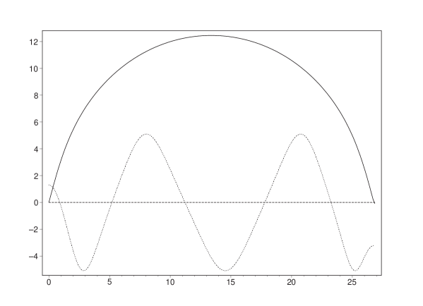
• $k=1$, closed universe. The only singular point is $a=0$, $b=0$ which is a center with the eigenvalues $\pm i\sqrt{6g}$, see the phase portrait in Fig. 1. All solutions are of an oscillating type: they start at the singularity ($a=0$) and after a stage of expansion shrink to another singularity. It is easy to see from (28) that the functions $a$ and $\dot{a}$ remain bounded for all solutions.

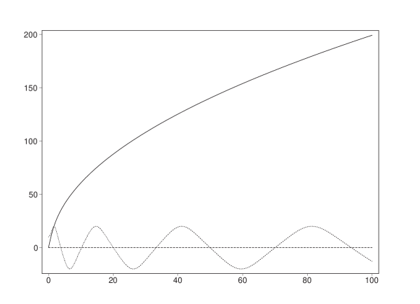
• $k=0$, spatially flat universe. There is a singular line $b=0$ each point of which represents a solution for an empty space (Minkowski spacetime). This set is degenerate, and there are no solutions that reach this curve for finite values of $a$ (see Fig. 2 for the phase portrait). All solutions in the upper half-plane after initial singularity expand infinitely.

  A remarkable fact is that for this case one can write an exact solution of (27) (in an implicit form):

  $$4\sqrt{g}\,(t-t_{0})=\sqrt{3}\left(\Omega-\arctan\Omega^{-1}+\pi/2\right),$$

  where $\Omega=\sqrt{2}\,a/\sqrt{\sqrt{a^{4}+C}-a^{2}}$. The metric singularity is reached at $t=t_{0}$.

• $k=-1$, open universe. There is a center at $a=0$, $b=0$ with the eigenvalues $\pm i\sqrt{6g}$, but it lies outside the boundary of the physical region. Other singular points are $(a=0,\;\;b=\pm 1)$ (Fig. 3). These points are degenerate and cannot be reached from any point lying in the physically allowed domain of the phase plane. The only solutions which start from them are the separatrices $b=\pm 1$ that represent (part of) the flat Minkowski spacetime in special coordinates.

  One can easily see that all solutions in the upper part of the physical domain $\dot{a}>1$ start from the singularity and then move to $a\to\infty$, $\dot{a}\to 1$.

The global qualitative behavior of solutions does not differ substantially from that in the conformally invariant YM field model, except near the singularity. One can find the following power series expansion near the singularity $a(0)=0$:

$$a(t)=b_{0}t-\frac{b_{0}g}{9}t^{3}+\frac{1}{270}\frac{b_{0}g^{2}(7b_{0}^{2}+k)}{(b_{0}^{2}+k)}t^{5}+O(t^{7}),\quad t\to 0,$$ (29)

where $b_{0}$ is a free parameter. Absence of the quadratic term means that the Universe starts with zero acceleration. This is what can be expected in view of the equation of state $p\approx-\varepsilon/3$ at high densities.

For large $a$, the dynamics of the system (18) approaches that of the hot FRW models (for small energy densities one recovers the equation of state of radiation).

5 Cosmological constant

Here we extend our analysis to the case of non-zero cosmological constant $\lambda$. This leads to the following one-dimensional action:

$$S_{1}=\frac{1}{4\pi G\beta}\int dt\left[\frac{3a}{2N}\left(kN^{2}-\dot{a}^{2}\right)+gNa^{3}\left(1-\sqrt{(1-K^{2})(1+V^{2})}-\frac{\lambda}{2g}\right)\right].$$

Clearly, the equations governing the gauge field dynamics (22) are unaffected by the cosmological term. The metric equations can be decoupled again using the constraint equation (14):

$$\ddot{a}=-\frac{1}{3}a(2g-\lambda)+\frac{4}{3}\frac{g^{2}a^{3}}{[(2g-\lambda)a^{2}+3(\dot{a}^{2}+k)]}.$$ (30)

The physical region of the phase space is defined by positivity of the energy of the gauge field (17), now the boundary being

$$\dot{a}^{2}-\frac{\lambda}{3}a^{2}+k\geq 0.$$ (31)

For the closed and spatially flat universes and a negative cosmological constant the allowed domain coincides with the whole plane $a,\dot{a}$. In other cases, there is a boundary corresponding to the solution with zero gauge field, i.e., the (anti)de-Sitter space.

The cosmological constant gives rise to new types of solutions including de-Sitter-like, which are non-singular. However, in the case when there is a singularity, its structure is determined by the leading term in the equation of state, namely, by the BI pressure, and is thus unaffected by the cosmological constant. The generic solution near the singularity satisfies the following series expansion

$$a(t)=b_{0}t-\frac{2g-\lambda}{18}b_{0}\,t^{3}+O(t^{5}),\quad t\to 0,$$ (32)

where $b_{0}$ is a free parameter. Again, the Universe starts with zero acceleration.

To proceed further with the analysis of Eq. (30), we rewrite it as the following two-dimensional dynamical system:

$$a^{\prime}=3\left[(2g-\lambda)a^{2}+3(b^{2}+k)\right]b,\qquad b^{\prime}=\left[\lambda(4g-\lambda)a^{2}-3(b^{2}+k)(2g-\lambda)\right]a,$$ (33)

where primes denote derivatives with respect to a new time variable $\tau$ defined by $dt=3[(2g-\lambda)a^{2}+3(b^{2}+k)]d\tau$. The system is symmetric under a simultaneous reflection of both variables, so we can think about a half of the phase space.

Similarly to the previous section, one may treat $b$ as a function of $a$ and thus obtain the first integral, which completely defines the integral curves of (33):

$$3\left(b^{2}-\frac{\lambda}{3}a^{2}+k\right)^{2}+4ga^{2}\left(b^{2}-\frac{\lambda}{3}a^{2}+k\right)=C.$$ (34)

Note that the terms in brackets are non-negative within the allowed domain (31).

The structure of the solution space can be revealed using this first integral. Let us start describing singular points of the dynamical system for different $k$.

• $k=1$, closed universe. For a negative cosmological constant the only singular point is $(a=0,b=0)$, which is a center with eigenvalues $\xi=\pm 3i\sqrt{3(2g-\lambda)}$. All phase space trajectories are deformed circles, and all solutions start from the singularity and reach the singularity in the future.

  For a positive cosmological constant, the allowed domain is bounded by a hyperbola $b^{2}-\frac{\lambda}{3}a^{2}>-1$ which represents the de-Sitter space.

  For relatively small $\lambda$ the point $(a=0,b=0)$ remains a center. At the same time, another pair of singular points appears:

  $$a=\pm\sqrt{\frac{3(2g-\lambda)}{\lambda(4g-\lambda)}},\qquad b=0.$$ (35)

  For $\lambda<2g$ they lie within the allowed domain and correspond to the static Einstein universe. These are saddle points with eigenvalues

  $$\xi=\pm\frac{6\sqrt{6}\,g}{\lambda}\sqrt{\frac{\lambda(2g-\lambda)}{4g-\lambda}}\,.$$

  Entering them separatrices correspond to either a solution developing from the singularity into the static universe, or one rolling down from an infinite radius to the static universe (Fig. 4). These separatrices divide the phase space into the domains containing different types of generic solutions. Near the origin, all solutions evolve from an initial to a final singularity. In the region near the physical boundary, the solutions are non-singular and evolve for an infinite time first shrinking to some finite value of the scale factor and then ever expanding. Generic solutions of the third type possess a singularity but are non-periodic: the universe expands forever.

  With $\lambda$ further increasing, the saddle point approaches the origin and finally, when $\lambda>2g$, swallows it. The character of the singular point $(a=0,b=0)$ changes—it becomes a saddle point ((Fig. 5). The separatrices entering it are solutions of an inflationary type. They divide all generic solutions into two classes: nonsingular de-Sitter-like (i.e., ever-expanding in the future and ever-contracting in the past) and ever-expanding solutions with an initial singularity. When $\lambda>4g$, the Eq. (35) has a real singular point lying outside the physical region.

• $k=0$, spatially flat universe. The only singular point is the origin $(a=0,b=0)$ which now is degenerate. For $\lambda<0$ the allowed domain is the whole plane. All solutions are of an oscillatory type evolving from the initial to the final singularity for a finite time.

  For a positive cosmological constant the allowed domain consists of the upper and lower parts of a cone $b^{2}-\frac{\lambda}{3}a^{2}>0$ whose boundary corresponds to the (part of) de-Sitter space described in the inflating coordinates. All solutions that lie within the allowed domain have an initial singularity and are ever expanding in the future.

• $k=-1$, open universe. The allowed domain (31) lies outside of either an ellipse ($\lambda<0$), or a hyperbola ($\lambda>0$).

  In this case two types of singular points—the origin and

  $$a=\pm\sqrt{\frac{3(\lambda-2g)}{\lambda(4g-\lambda)}},\qquad b=0$$ (36)

  (when they are real) lie outside the allowed domain and hence are of no interest.

  Another pair of singular points is $(a=0,b=\pm 1)$. These are degenerate (as in case with zero cosmological constant). Since they lie on the boundary of the allowed domain, the only physical solutions approaching them correspond to zero energy of the BI field ((anti)-deSitter).

  All generic solutions within the allowed domain possess a singularity and are either oscillating (for $\lambda<0$) or ever expanding (for $\lambda>0$).

6 Dynamics of the gauge field

One can easily see that the gauge field influences the metric only through the quantity $\mathcal{P}$ (15), related to the energy density. This quantity obeys the differential equation:

$$\dot{}\mathcal{P}=2\frac{\dot{a}}{a}\left(\frac{1}{\mathcal{P}}-\mathcal{P}\right),$$ (37)

which follows from (22) and does not depend either on a detailed YM dynamics, or a particular gauge choice (e.g., $N=1$, or $N=a$). This equation can be integrated once, giving $\mathcal{P}$ as a function of $a$:

$$\mathcal{P}=\sqrt{1+3\left(\frac{a_{0}}{a}\right)^{4}},$$ (38)

where $a_{0}$ is an integration constant, and a numerical coefficient was introduced for future convenience. This equation gives us a possibility to fully describe the gauge field dynamics. Recalling the definition of $\mathcal{P}$ (15), one can separate the metric and the gauge field variables as follows:

$$\frac{\dot{w}^{2}}{a_{0}^{4}-(k-w^{2})^{2}}=\frac{N^{2}a^{2}}{a^{4}+3a_{0}^{4}}.$$ (39)

Since the right hand side of this equation is strictly positive, we can find the domain of variation of the function $w$. It is symmetric with respect to $w\to-w$, except for the case $a_{0}<1$, $k=1$, when $w$ oscillates near the value $w=1$ (or $w=-1$) without crossing the axis $w=0$.

The equation (39) can be solved in terms of the Jacobi elliptic functions, similarly to the case of an ordinary YM lagrangian [23]:

$$w(t)=\sqrt{k+a_{0}^{2}}\mathop{\mathrm{cn}}\left(\sqrt{2}a_{0}(\tau-\tau_{0}),\frac{\sqrt{k+a_{0}^{2}}}{\sqrt{2}a_{0}}\right),$$ (40)

where $\tau_{0}$ is the integration constant, and the argument to the Jacobi function is defined as

$$\tau(t)=\int^{t}\frac{a(t^{\prime})N(t^{\prime})\,dt^{\prime}}{\sqrt{a^{4}(t^{\prime})+3a_{0}^{4}}}.$$ (41)

A generic solution for $w(t)$ is of an oscillating type. In the case $a_{0}<1$, $k=1$, the solution, oscillating near one of the values $w=\pm 1$, does not cross the line $w=0$. In all other cases solutions oscillate around the origin. The effective frequency of oscillations is determined by the rate of growth of the argument $\tau$. To compare the situation with the ordinary EYM cosmology, we notice that in this case the solution for $w(t)$ is still given by (40), but with a different definition of the phase variable $\tau(t)$ [23]

$$\tau_{EYM}(t)=\int^{t}\frac{N(t^{\prime})}{a(t^{\prime})}\,dt^{\prime}.$$

Clearly, the main difference with the ordinary EYM cosmology relates to small values of $a$. One can see that near the singularity ($a\to 0$) the YM oscillations in the NBI case slow down, while in the ordinary YM cosmology the frequency remains constant in the conformal gauge $N=a$, or tends to infinity in proper time gauge $N=1$. The behavior of the YM field for closed and spatially flat models is illustrated in Figs.(6,7).

When the solution starts from the metric singularity, the gauge field function has the following series expansion (the metric is supposed to satisfy the expansion (32)).

$$w=w_{0}+\frac{b_{0}\alpha}{6(k+b_{0}^{2})}t^{2}+\left(\frac{g^{2}b_{0}^{2}w_{0}(k-w_{0}^{2})}{9(k+b_{0}^{2})^{2}}+\frac{b_{0}\alpha(\lambda-2g)}{216(k+b_{0}^{2})}\right)t^{4}+O(t^{6}),\quad t\to 0,$$ (42)

where $\alpha=\pm\sqrt{3(k+b_{0}^{2})^{2}-4g^{2}(k-w_{0}^{2})^{2}}$, $w_{0}$ is a free parameter (as well as the sign of $\alpha$), while $b_{0}$ is a parameter from the expansion of the metric (32).

7 Discussion

In spite of considerable complications which the Born–Infeld non-linearity introduces to the Einstein–Yang–Mills coupled equations, the dynamics of the FRW NBI cosmology turned out to be separable and admitting a rather complete analysis in terms of the dynamical systems theory. This is due to the fact that the NBI YM equation admits a first integral expressing the variation of the energy density under cosmological evolution. Thus one obtains a decoupled equation for the scale factor both without or with the cosmological constant. We have given a rather complete classification of possible solutions for closed, spatially flat, and open universes in these cases.

One of the intriguing features associated with the NBI theory is the possibility of a negative pressure. Namely, the pressure is negative when the field energy density exceeds the ’critical’ BI energy density. This is still insufficient to mimic an inflation, since the lowest value is only $p=-\varepsilon/3$, which coincides with the equation of state of the gas of Nambu-Goto strings in three spatial dimensions. In the framework of the FRW cosmology, the equation of state of the NBI YM field continuously interpolates from $p=-\varepsilon/3$ near the singularity to the ‘radiation’ equation $p=\varepsilon/3$ at large time. Correspondingly, the energy density is evolving near the singularity according to the law $a^{-2}$. The FRW NBI universe starts with zero acceleration and achieves the Tolman expansion regime, when the energy density is diluted sufficiently to make the Born–Infeld non-linearity negligible.

Once the scale factor evolution is determined, one is able to find an analytic solution for the YM function is terms of elliptic functions. Qualitatively the YM dynamics remains the same as in the usual YM theory, though we have observed that near the singularity the oscillations of the YM field are damped.

Figure 1: Phase portrait of the dynamical system for the closed NBI universe.

Figure 2: Phase portrait of the dynamical system for the spatially flat NBI universe.

Figure 3: Phase portrait of the dynamical system for the open NBI universe. Physical domain in this case is $-1<b<1$.

Figure 4: Phase portrait of the dynamical system (33) for the closed NBI universe with a cosmological constant $0<\lambda<2g$. Physical domains are bounded by hyperbolas plotted in dashed line.

Figure 5: Phase portrait of the dynamical system (33) for the closed NBI universe with a cosmological constant $\lambda>2g$.

Figure 6: Sample solution for the closed universe filled by the NBI YM field. Dotted line—gauge field function $w$, solid line—metric function $a$. The values of parameters are $g=\frac{1}{2}$, $C=5$, $w_{0}=1.3$.

Figure 7: Sample solution for the spatially flat universe with NBI YM field. Dotted line—gauge field function $w$, solid line—metric function $a$.

References

- [1] Ricardo Garcia-Salcedo and Nora Breton. Born–Infeld cosmologies. Int. J. Mod. Phys., A15:4341–4354, 2000, gr-qc/0004017.
- [2] B. L. Altshuler. An alternative way to inflation and the posibility of anti-inflation. Class. Quant. Grav., 7:189–201, 1990.
- [3] Dan N. Vollick. Anisotropic Born–Infeld cosmologies. 2001, hep-th/0102187.
- [4] J Cervero and L Jacobs. Classical Yang–Mills fields in a Robertson–Walker universe. Phys. Lett., B 78:427–429, 1978.
- [5] M. Henneaux. Remarks on space-time symmetries and nonabelian gauge fields. J. Math. Phys., 23:830, 1982.
- [6] Y. Verbin and A. Davidson. Quantized nonabelian wormholes. Phys. Lett., B229:364, 1989.
- [7] D. V. Gal’tsov and M. S. Volkov. Yang–Mills cosmology: Cold matter for a hot universe. Phys. Lett., B256:17–21, 1991.
- [8] G. W. Gibbons and Alan R. Steif. Yang–Mills cosmologies and collapsing gravitational sphalerons. Phys. Lett., B320:245–252, 1994, hep-th/9311098.
- [9] Mikhail S. Volkov. Einstein Yang–Mills sphalerons and fermion number nonconservation. Phys. Lett., B328:89–97, 1994, hep-th/9312005.
- [10] S.X. Ding. Cosmological sphaleron with real tunneling and its fate. Phys. Rev., D50:3755–3759, 1994.
- [11] T. Hagiwara. A nonabelian Born–Infeld lagrangian. J. Phys., A14:3059, 1981.
- [12] A. A. Tseytlin. On non-abelian generalisation of the Born–Infeld action in string theory. Nucl. Phys., B501:41–52, 1997, hep-th/9701125.
- [13] A. A. Tseytlin. Born–Infeld action, supersymmetry and string theory. 1999, hep-th/9908105.
- [14] Jeong-Hyuck Park. A study of a non-Abelian generalization of the Born–Infeld action. Phys. Lett., B458:471, 1999, hep-th/9902081.
- [15] Akikazu Hashimoto and IV Taylor, Washington. Fluctuation spectra of tilted and intersecting D-branes from the Born–Infeld action. Nucl. Phys., B503:193–219, 1997, hep-th/9703217.
- [16] Andrea Refolli, Alberto Santambrogio, Niccolo Terzi, and Daniela Zanon. contributions to the nonabelian Born–Infeld action from a supersymmetric Yang–Mills five-point function. Nucl. Phys., B613:64–86, 2001, hep-th/0105277.
- [17] Adel Bilal. Higher-derivative corrections to the non-abelian Born–Infeld action. 2001, hep-th/0106062.
- [18] E. A. Bergshoeff, A. Bilal, M. de Roo, and A. Sevrin. Supersymmetric non-abelian Born–Infeld revisited. JHEP, 07:029, 2001, hep-th/0105274.
- [19] Alexander Sevrin, Jan Troost, and Walter Troost. The non-abelian Born–Infeld action at order . Nucl. Phys., B603:389–412, 2001, hep-th/0101192.
- [20] Dmitri Gal’tsov and Richard Kerner. Classical glueballs in non-Abelian Born–Infeld theory. Phys. Rev. Lett., 84:5955–5958, 2000, hep-th/9910171.
- [21] V. V. Dyadichev and D. V. Gal’tsov. Solitons and black holes in non-Abelian Einstein–Born–Infeld theory. Phys. Lett., B486:431–442, 2000, hep-th/0005099.
- [22] Edward Witten. Some exact multipseudoparticle solutions of classical Yang- Mills theory. Phys. Rev. Lett., 38:121, 1977.
- [23] E. E. Donets and D. V. Galtsov. Continuous family of Einstein Yang–Mills wormholes. Phys. Lett., B294:44–48, 1992, gr-qc/9209008.