Effective Gravitational Field of Black Holes

Abstract

The problem of interpretation of the $\hbar^{0}$-order part of radiative corrections to the effective gravitational field is considered. It is shown that variations of the Feynman parameter in gauge conditions fixing the general covariance are equivalent to spacetime diffeomorphisms. This result is proved for arbitrary gauge conditions at the one-loop order. It implies that the gravitational radiative corrections of the order $\hbar^{0}$ to the spacetime metric can be physically interpreted in a purely classical manner. As an example, the effective gravitational field of a black hole is calculated in the first post-Newtonian approximation, and the secular precession of a test particle orbit in this field is determined.

I Introduction

The question of interpretation of quantum gravity calculations is one of the most difficult in quantum field theory. Apart from difficulties caused by the formal inapplicability of basic notions of the flat space theory, such as the asymptotic states in the standard S-matrix approach, the very notion of classical limit in the quantum theory of gravitation, underlying the issue of interpretation, is essentially different from that in other theories of fundamental interactions. It cannot be formulated neither as the large mass limit of interacting particles, since the gravitational radiative corrections do not disappear in this limit [1], nor even as the formal limit $\hbar\to 0:$ as was shown in Refs. [2, 3], the first post-Newtonian correction to the gravitational potential, given by the quantum theory, is twice as large as that given by the Schwarzschild solution of the classical theory.

It was suggested in Refs. [2, 3] that the correct correspondence between classical and quantum theories is to be established not for fundamental particles described by field operators entering the action functional, but rather for macroscopic bodies consisting of a large number of such particles. This interpretation of the correspondence principle is underlined by an observation that the $n$-loop radiative contribution to the $n$th post-Newtonian correction to the gravitational field of a body with mass $M,$ consisting of $N=M/m$ elementary particles with mass $m,$ contains an extra factor of $1/N^{n}$ in comparison with the corresponding tree contribution. Thus, the effective gravitational field produced by the body turns into the classical solution of the Einstein equations in the limit $N\to\infty$ (and therefore, $M\to\infty$). An immediate consequence of this interpretation is that in the case of finite $N,$ the loop corrections of the order $\hbar^{0}$ describe deviations of the spacetime metric from classical solutions of the Einstein equations.

To justify this interpretation completely, one has to prove its gauge-independence, i.e., that arbitrariness in the choice of gauge conditions fixing the general covariance does not make values of measurable quantities, built from the effective metric, ambiguous. In Ref. [2], independence of the gauge parameter, weighting the DeWitt gauge conditions in the action, was proved by direct calculation at the one-loop order. The purpose of this Letter is to show that this result is not accidental, and to prove it in a much more simple and general way for arbitrary gauge conditions. After that, application to the black holes will be discussed.

II Gauge dependence of $\hbar^{0}$ one-loop corrections

Let us consider a body with mass $M$ consisting of an arbitrary number $N$ of particles. For simplicity the latter will be assumed identical scalars with mass $m,$ denoted by $\phi.$ Dynamics of the field $\phi$ is described by the action

$$S_{\phi}=\frac{1}{2}{\displaystyle\int}d^{4}x\sqrt{-g}\left\{g^{\mu\nu}\partial_{\mu}\phi\partial_{\nu}\phi-\left(\frac{mc}{\hbar}\right)^{2}\phi^{2}\right\},$$ (1)

while the action for the gravitational field

$$S=-\frac{c^{3}}{k^{2}}{\displaystyle\int}d^{4}x\sqrt{-g}R,$$ (2)

where $k^{2}=16\pi G,$ $G$ being the Newton gravitational constant.

The action $S+S_{\phi}$ is invariant under the following gauge transformations

$$\delta h_{\mu\nu} = \xi^{\alpha}\partial_{\alpha}h_{\mu\nu}+(\eta_{\mu\alpha}+h_{\mu\alpha})\partial_{\nu}\xi^{\alpha}+(\eta_{\nu\alpha}+h_{\nu\alpha})\partial_{\mu}\xi^{\alpha}\equiv D_{\mu\nu}^{\alpha}(h)\xi_{\alpha},$$ (3)

$$~{}~{}\delta\phi = \xi^{\alpha}\partial_{\alpha}\phi\equiv D^{\alpha}(\phi)\xi_{\alpha},$$ (4)

where $\xi^{\alpha}$ are the (infinitesimal) gauge functions. Let this invariance be fixed by the following conditions

$$F_{\alpha}(h)=0.$$ (5)

For the beginning, $F_{\alpha}$ will be assumed linear,

$$F_{\alpha}(h)\equiv F^{\mu\nu}_{\alpha}h_{\mu\nu},$$ (6)

where $F_{\alpha}^{\mu\nu}$ are some differential operators (Lorentz covariant or not) independent of the fields $h_{\mu\nu}.$ The most general case will be considered later. Weighted in the usual way, gauge conditions enter the Faddeev-Popov action

$$S_{\rm FP}=S+S_{\phi}+S_{\rm gf}+\bar{C}^{\beta}F_{\beta}^{\mu\nu}D_{\mu\nu}^{\alpha}C_{\alpha}$$ (7)

in the form of the gauge fixing term

$$S_{\rm gf}=\frac{1}{2\xi}F_{\alpha}F^{\alpha},$$ (8)

where $\xi$ is the Feynman gauge parameter, and $C_{\alpha},\bar{C}^{\alpha}$ are the Faddeev-Popov ghosts.

Let us now turn to examination of the radiative corrections. Since we are interested in the quantum contribution to the first post-Newtonian correction, the only diagram we need to consider is the one-loop diagram pictured in Fig. 1. As a simple dimensional analysis shows, other one-loop diagrams do not contain root singularities $1/\sqrt{-p^{2}}$ corresponding to the $\hbar^{0}$-contribution, while the higher-loop diagrams are of higher orders in the Newton constant. Note that it is the propagation of virtual scalar particle near its mass shell which is responsible for the occurrence of the $\hbar^{0}$-contribution.

Although direct calculation of this diagram is cumbersome, the question of the $\xi$-dependence of its $\hbar^{0}$ contribution can be easily analyzed as follows.

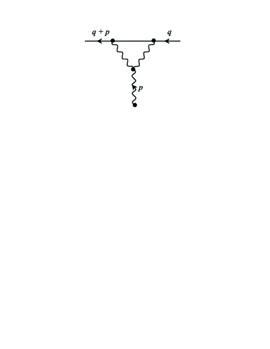
FIG. 1.: The one-loop diagram contributing to the first post-Newtonian correction. Wavy lines represent gravitons, full lines scalar particles; $q$ and $p$ are the 4-momentum of the scalar particle and the momentum transfer, respectively.

In the linear gauge (6), gauge dependence of this diagram is determined by that of the graviton propagators. If the graviton propagator is defined by

$$\frac{\delta^{2}S}{\delta h_{\rho\tau}\delta h_{\mu\nu}}G_{\mu\nu\zeta\lambda}=-\delta_{\zeta\lambda}^{\rho\tau}\,,$$ (9)

$$~{}~{}\delta_{\zeta\lambda}^{\rho\tau}=\frac{1}{2}(\delta_{\zeta}^{\rho}\delta_{\lambda}^{\tau}+\delta_{\zeta}^{\tau}\delta_{\lambda}^{\rho})\,,$$ (10)

then its $\xi$-derivative

$$\frac{\partial G_{\mu\nu\zeta\lambda}}{\partial\xi}=G_{\mu\nu\alpha\beta}\frac{F_{\sigma}^{\alpha\beta}F^{\sigma,\gamma\delta}}{2\xi^{2}}G_{\gamma\delta\zeta\lambda}\,.$$ (11)

On the other hand, multiplying definition (9) by the generator $D^{(0)\alpha}_{\rho\tau}\equiv D^{\alpha}_{\rho\tau}(h=0),$ one has

$$F^{\alpha,\mu\nu}G_{\mu\nu\sigma\lambda}=\xi D^{(0)\beta}_{\sigma\lambda}\tilde{G}_{\beta}^{\alpha}\,,$$ (12)

where $\tilde{G}_{\beta}^{\alpha}$ is the ghost propagator satisfying

$$F_{\alpha}^{\mu\nu}D^{(0)\beta}_{\mu\nu}\tilde{G}^{\gamma}_{\beta}=-\delta_{\alpha}^{\gamma}\,.$$ (13)

Let us first consider the inner propagators in Fig. 1. In view of Eqs. (11), (12), $\xi$-dependent terms in these propagators are attached to the scalar line through the generator $D^{(0)\alpha}_{\mu\nu}.$ On the other hand, the action $S_{\phi}$ is invariant with respect to the gauge transformations (3),

$$\frac{\delta S_{\phi}}{\delta\phi}D^{\alpha}(\phi)+\frac{\delta S_{\phi}}{\delta h_{\mu\nu}}D^{\alpha}_{\mu\nu}(h)=0.$$ (14)

Differentiating this identity with respect to $\phi,$ setting $h_{\mu\nu}=0,$ and taking into account that the external scalar lines are on the mass shell

$$\left.\frac{\delta S_{\phi}}{\delta\phi}\right|_{h=0}=0,$$

each of the two $\phi-h-\phi$ vertices can be written as

$$\left.\frac{\delta^{2}S_{\phi}}{\delta\phi\delta h_{\mu\nu}}\right|_{h=0}D^{(0)\alpha}_{\mu\nu}=-\left.\frac{\delta^{2}S_{\phi}}{\delta\phi^{2}}\right|_{h=0}D^{\alpha}(\phi).$$ (15)

Thus, under contraction with the vertex factor, the scalar particle propagator, $G_{\phi},$ satisfying

$$\left.\frac{\delta^{2}S_{\phi}}{\delta\phi^{2}}\right|_{h=0}G_{\phi}=-1,$$

cancels out

$$G_{\phi}\left.\frac{\delta^{2}S_{\phi}}{\delta\phi\delta h_{\mu\nu}}\right|_{h=0}D^{(0)\alpha}_{\mu\nu}=D^{\alpha}(\phi).$$ (16)

We conclude that the $\hbar^{0}$ contribution to the one-particle-irreducible part of Fig. 1 is $\xi$-independent. Now, using Eqs. (11) and (12) in the external propagator, we see that the $\xi$-derivative of the corresponding contribution to the whole diagram is proportional to the generator $D^{(0)\alpha}_{\mu\nu}.$ In other words, variations of the Feynman parameter induce spacetime diffeomorphisms.

This important result allows us to interpret the $\hbar^{0}$-part of the radiative corrections in a purely classical manner. It was mentioned above that the loop corrections to the spacetime metric can be endowed with physical meaning only if their gauge dependence does not introduce an ambiguity into the values of measurable quantities. The latter are generally defined as functionals of the field variables, invariant with respect to the spacetime diffeomorphisms. Since we presently deal with the first post-Newtonian correction, this criterion can be written

$$\frac{\delta O}{\delta g^{\rm eff}_{\mu\nu}}D^{\alpha}_{\mu\nu}(h^{\rm eff})\approx\frac{\delta O}{\delta g^{\rm eff}_{\mu\nu}}D^{(0)\alpha}_{\mu\nu}=0,~{}~{}h^{\rm eff}_{\mu\nu}=g^{\rm eff}_{\mu\nu}-\eta_{\mu\nu},$$

where $O$ is any observable, and $g^{\rm eff}_{\mu\nu}$ the effective metric field. We thus see that variations of the Feynman parameter do not affect values of the observables. This is as it should be, since, unlike other gauge parameters entering the gauge conditions $F_{\alpha}$ and determining structure of a given coordinate system, the weighting parameter $\xi$ does not have any geometrical meaning. Furthermore, using the $\xi$-independence of observables, one can put $\xi=0.$ Then Eq. (12) shows that the effective metric can always be chosen to satisfy the gauge conditions exactly,

$$F_{\alpha}(h^{\rm eff})=F_{\alpha}^{\mu\nu}h^{\rm eff}_{\mu\nu}=0.$$

Finally, let us consider the most general case of nonlinear gauge conditions. The gauge fixing term has the form

$$S_{\rm gf}=\frac{F^{\alpha}F_{\alpha}}{2\xi}=\frac{\tilde{F}^{\alpha}\tilde{F}_{\alpha}}{2\xi}+\frac{\tilde{F}^{\alpha}f_{\alpha}}{\xi}+\frac{f^{\alpha}f_{\alpha}}{2\xi},$$ (17)

where $\tilde{F}_{\alpha}$ is the linear part of $F_{\alpha},$ having the form (6), and $f_{\alpha}$ is of higher orders in the fields $h_{\mu\nu},$ responsible for the appearance of new, “fictitious” interactions of gravitons. At the one-loop order, there is only one new diagram, of the type shown in Fig. 1, in which the triple graviton vertex is generated by the second term in the right hand side of Eq. (17). It is easy to see that the effect of addition of this diagram is again a spacetime diffeomorphism. Indeed, if the factor $\tilde{F}_{\alpha}$ acts on one of the internal graviton lines, using Eq. (12) and repeating literally the reasoning which led to Eq. (16), we see that the $\hbar^{0}$-terms fall out of the diagram. If the factor $\tilde{F}_{\alpha}$ acts on the external graviton line, the use of Eq. (12) shows that the corresponding contribution is proportional to $D^{(0)\alpha}_{\mu\nu}.$

Thus, variations of the Feynman parameter are proved to be equivalent to spacetime diffeomorphisms for the most general gauge conditions.

III Effective gravitational field of black holes

It was mentioned in the Introduction that in comparison with the classical general relativity, the one-loop contribution to the first post-Newtonian correction to the gravitational field of a macroscopic body consisting of $N$ particles is suppressed by the factor $1/N.$ For instance, if the gauge condition is that of DeWitt

$$F_{\alpha}=\partial^{\mu}h_{\mu\alpha}-\frac{1}{2}\partial_{\alpha}h,~{}~{}h\equiv\eta^{\mu\nu}h_{\mu\nu},$$ (18)

the gravitational potential of a spherically symmetric body with mass $M$ is [2]

$$\Phi(r)=-\frac{GM}{r}+\frac{G^{2}M^{2}}{2c^{2}r^{2}}-\frac{G^{2}M^{2}}{Nc^{2}r^{2}}\,.$$ (19)

This suppression of the quantum contribution guaranties that the classical predictions of general relativity are in agreement with observations of motion of macroscopic bodies (for the solar gravitational field, for instance, $1/N\approx m_{\rm proton}/M_{\odot}\approx 10^{-57}$).

As was explained in Ref. [2], gravitational interaction of the constituent particles is taken into account in Eq. (19), up to terms of higher order in $G,$ by identifying $M$ as the gravitational mass of the body. This is legitimate only if the interaction is not too strong, namely, if its expansion in powers of $G$ is justified.

Let us now consider a situation when evolution of the system of particles ends up with formation of the horizon. Then the above condition on the strength of particle interaction inevitably breaks down at some stage. In the absence of self-consistent quantum theory of gravitation, nothing can be said about the ultimate fate of the collapsing matter. What can be said, however, is that from the point of view of external observer, the number $N$ is now irrelevant to the gravitational field of the collapsar (this is a consequence of the “no hair” theorem). Made by the infinite gravitational force indivisible, this object can be considered as a “particle”. I will assume that it can be described by a scalar field with mass $M$ equal to the gravitational mass of the black hole. Then the one-loop contribution of the order $\hbar^{0}$ to the gravitational field of the black hole, represented in Fig. 1, is [2]

$$h^{{\rm loop}}_{\mu\nu}(p)=-\frac{\pi^{2}G^{2}}{c^{2}\sqrt{-p^{2}}}\left(3M^{2}\eta_{\mu\nu}+\frac{q_{\mu}q_{\nu}}{c^{2}}+7M^{2}\frac{p_{\mu}p_{\nu}}{p^{2}}\right).$$ (20)

Written down in the coordinate space with the help of the formulae

$$\int\frac{d^{3}{\bf p}}{(2\pi)^{3}}\frac{e^{i{\bf px}}}{|{\bf p}|} = \frac{1}{2\pi^{2}r^{2}}\,,$$ (21)

$$\int\frac{d^{3}{\bf p}}{(2\pi)^{3}}\frac{p_{i}p_{k}}{|{\bf p}|^{3}}e^{i{\bf px}} = \frac{1}{2\pi^{2}r^{2}}\left(\delta_{ik}-\frac{2x_{i}x_{k}}{r^{2}}\right),~{}~{}r^{2}\equiv\delta_{ik}x^{i}x^{k}\,,$$ (22)

equation (20) gives, in the static case,

$$h^{\rm loop}_{00}=-\frac{2G^{2}M^{2}}{c^{2}r^{2}}\,,~{}~{}h^{{\rm loop}}_{ik}=\frac{G^{2}M^{2}}{c^{2}r^{2}}\left(-2\delta_{ik}+\frac{7x_{i}x_{k}}{r^{2}}\right).$$ (23)

In order to find complete expression for the metric in the first post-Newtonian approximation, one has to add the tree contribution, given by the Schwarzschild solution transformed to the DeWitt gauge condition (18) under which Eqs. (23) were derived. Using Eq. (4) of Ref. [2], we thus obtain the following expression for the interval

$$ds^{2}\equiv g^{\rm eff}_{\mu\nu}dx^{\mu}dx^{\nu}=\left(1-\frac{r_{g}}{r}\right)c^{2}dt^{2}-\left(1+\frac{r_{g}}{r}-\frac{7r^{2}_{g}}{4r^{2}}\right)dr^{2}$$ (24)

$$-r^{2}\left(1+\frac{r_{g}}{r}+\frac{7r^{2}_{g}}{4r^{2}}\right)(d\theta^{2}+\sin^{2}\theta\ d\varphi^{2}),$$ (25)

where $\theta,\phi$ are the standard spherical angles, and $r_{g}=2GM/c^{2}.$

As an application of the obtained result, let us consider one of the classic effects of general relativity, the orbit precession in the gravitational field of a spherically symmetric body. Let a test particle with mass $m$ move in the equatorial plane ($\theta=\pi/2$) around black hole. Denoting $S_{\rm b}$ the action of the body, we write the Hamilton-Jacobi equation

$$g^{\mu\nu}_{\rm eff}\frac{\partial S_{\rm b}}{\partial x^{\mu}}\frac{\partial S_{\rm b}}{\partial x^{\nu}}-m^{2}c^{2}=0,$$

where $g^{\mu\nu}_{\rm eff}$ is the inverse of $g_{\mu\nu}^{\rm eff}.$ A simple calculation gives, to the leading order,

$$S_{\rm b} = -Et+L\varphi$$ (26)

$$+ \int dr\left[\left(\frac{E^{\prime 2}}{c^{2}}+2mE^{\prime}\right)+\frac{r_{g}}{r}\left(m^{2}c^{2}+4mE^{\prime}\right)-\frac{1}{r^{2}}\left(L^{2}-2r_{g}^{2}m^{2}c^{2}\right)\right]^{1/2},$$ (27)

where $E,L$ are the energy and angular momentum of the particle, respectively, and $E^{\prime}=E-mc^{2}$ its non-relativistic energy. The first two terms in the integrand in Eq. (26) coincide with the corresponding terms of classical theory, while the third does not, leading to the angular shift of the perihelion

$$\delta\varphi=\frac{8\pi GM}{c^{2}a(1-e^{2})}$$ (28)

per period ($a$ and $e$ are the major semiaxis and the eccentricity of the orbit, respectively), which is to be compared with the classic result

$$\delta\varphi=\frac{6\pi GM}{c^{2}a(1-e^{2})}\ .$$

IV Conclusions

Interpretation of the correspondence principle, suggested in Ref. [2], endows the $\hbar^{0}$ loop contributions with direct physical meaning as describing deviations of the spacetime metric from classical solutions of the Einstein equations. This purely classical treatment of the $\hbar^{0}$ loop contributions is supported by the main result of the present work: variations of the weighting parameter are equivalent to spacetime diffeomorphisms. Thus, observables built from the effective metric are independent of the unphysical Feynman parameter. As to other gauge parameters entering the gauge conditions $F_{\alpha}$ and determining geometry of a given coordinate system, the corresponding analysis is much more complicated and will be presented elsewhere.

It should be clear from the considerations of Sec. II that this result is valid whatever matter fields produce the gravitational field. In essential, it is a consequence of the gauge symmetry of the action $S+S_{\phi}.$ Despite simplicity of the proof at the one-loop order, however, the author has not yet been able to extend it to all orders.

As an application of this result, the one-loop effective gravitational field of black hole was calculated. It is given by Eq. (24). One of the consequences is that the orbit precession in this field differs from that predicted by the classical Einstein theory, and is given by Eq. (28). It should be mentioned in this connection that emission of the gravitational waves by the black hole binaries also must be affected by the quantum contributions. The LIGO and VIRGO gravitational wave detectors, which are currently under construction, will hopefully bring light into this issue.

- [1] J. F. Donoghue, Phys. Rev. Lett. 72, 2996 (1994); Phys. Rev. D50, 3874 (1994); Perturbative Dynamics of Quantum General Relativity, invited plenary talk at the ”Eighth Marcel Grossmann Conference on General Relativity”, Jerusalem (1997).
- [2] K. A. Kazakov, Class. Quantum Grav. 18, 1039 (2001).
- [3] K. A. Kazakov, Nucl. Phys. Proc. Suppl. 104, 232 (2002).