\recdate

Quantum Creation of the Randall-Sundrum Bubble

Hirotaka Ochiai1    Daisuke Ida2 and Tetsuya Shiromizu3 1Department of Physics1Department of Physics The University of Tokyo The University of Tokyo Tokyo 113-0033
2,3 Research Center for the Early Universe (RESCEU) Tokyo 113-0033
2,3 Research Center for the Early Universe (RESCEU) The University of Tokyo The University of Tokyo Tokyo 113-0033 Tokyo 113-0033
Abstract

We investigate the semiclassical instability of the Randall-Sundrum brane world. We carefully analyze the bubble solution with the Randall-Sundrum background, which expresses the decay of the brane world. We evaluate the decay probability following the Euclidean path integral approach to quantum gravity. Since a bubble rapidly expands after the nucleation, the entire spacetime will be occupied by such bubbles.

1 Introduction

In the nonperturbative approach to string theory, it is becoming accepted that the standard model particles are confined to branes. [1] This idea has led to the so-called brane-world scenario of the universe. The simplest models describing this scenario have been proposed by Randall and Sundrum. [2, 3] Therein, the four-dimensional Minkowski brane is located at the boundary of the five-dimensional anti-de Sitter (adS) space-time. The first Randall-Sundrum model (RS1) was motivated by the hierarchy problem and consists of two 3-branes [2]. The second Randall-Sundrum model (RS2) consists of a single 3-brane. [3] It has been shown that four-dimensional gravity, not five-dimensional gravity, is recovered at low energy scales on the branes. [4, 5] This represents a new type of dimensional reduction that is an alternative to the Kaluza-Klein compactification. In this way, possibility of realizing noncompact extra dimensions arises. The RS models can describe standard cosmology at low energy scales. There are indeed exact solutions describing the homogeneous and isotropic expanding universe. [6] Moreover, the RS brane world has comprehensive features, e.g., the adS/CFT interpretation. [7]

Although RS models have had great success, there are still fundamental questions regarding the stability. There are mainly two problems with RS1 models. One involves the radius stabilizations: In order to recover the correct four-dimensional gravity, we must assume that the distance between branes is stabilized. [8] A toy model for the stabilization problem has been proposed by Goldberger and Wise. [9]

The stability problem that we consider in the present paper concerns a quantum process. In the unified Kaluza-Klein theory, it is well known that the Kaluza-Klein vacuum is unstable with respect to the decay channel to the Kaluza-Klein bubble space-time. [10, 11] It may be thought that there is a similar instability of the RS model. This was first pointed out in Refs. [12] and  [13]. The discovery of an explicit example describing a sort of Kaluza-Klein bubble in the RS1 model (the RS bubble) was reported in a previous paper.[14] (A somewhat relevant solution is presented in Ref. [15]) In order to make the RS model feasible, this decay channel must be suppressed in some way. The purpose of this paper is to estimate the transition rate of the RS vacuum to the RS bubble in the framework of the Euclidean path integral procedure.

The remainder of this paper is organized as follows. In §2, we briefly review the RS bubble space-time. In §3, we calculate the transition probability of the RS vacuum to the RS bubble spacetime. In §4 we summarize the present work. For simplicity, we will set the five-dimensional gravitational scale to unity: $G_{5}=\kappa_{5}^{2}=1$.

2 Randall-Sundrum bubble

Here we briefly review the Randall-Sundrum bubble introduced in a previous paper. [14] The RS model of a two brane system (RS1) [2] is given by the metric

$$g=dy^{2}+e^{-2y/\ell}\eta_{\mu\nu}dx^{\mu}dx^{\nu},$$ (1)

where $\eta_{\mu\nu}$ is the four-dimensional Minkowski metric and $0\leq y\leq y_{0}$. The metric (1) is that of the five-dimensional adS space, and positive and negative tension branes are located at $y=0$ and $y=y_{0}$, respectively. The tension $\lambda$ of the ($\pm$)-branes are given by $\pm 6/\ell$, and the extrinsic curvatures on the branes are given by

$$K_{\mu\nu}:=\frac{1}{2}\mbox{\pounds}_{n}h_{\mu\nu}=\mp\frac{1}{\ell}h_{\mu\nu},$$ (2)

where $n=\pm\partial_{y}$ is the outward unit vector normal to the boundary and $h_{\mu\nu}=e^{-2y/\ell}\eta_{\mu\nu}$.

If the four-dimensional metric $\eta_{\mu\nu}$ is replaced by a Ricci-flat metric $q_{\mu\nu}$, then Eq. (1) represents a more generic Einstein metric. Let us write the brane-metric in the form

$$q=-r^{2}d\tau^{2}+dr^{2}+r^{2}\cosh^{2}\tau d\Omega_{2}{}^{2},$$ (3)

where $d\Omega_{2}{}^{2}$ denotes the standard metric of the unit two-sphere. The metric (3) represents the spherical Rindler space, which is locally flat but geodesically incomplete at the null hypersurface $r=0$ (Rindler horizon). Each $r={\rm constant}$ hypersurface corresponds to a world sphere in a uniformly accelerating expansion. We here consider another generalization of Eq. (1) with the same asymptotic behavior as Eq. (3) on the brane. This is given by 111Carrying out the signature change of $\Lambda$ and the double Wick rotation [$\Lambda\to-\Lambda,y\to it$ and $\tau\to i(\theta+\pi/2)$], it is found that this metric describes the five-dimensional Schwarzshild-deSitter space-time in isotropic coordinates. For investigation of four and higher dimensional cases, see Refs. [16] and  [17].

$\displaystyle g=\left[\frac{1-(\rho_{*}/ar)^{2}}{1+(\rho_{*}/ar)^{2}}\right]^{2}dy^{2}+a^{2}\left[1+\left(\frac{\rho_{*}}{ar}\right)^{2}\right]^{2}(-r^{2}d\tau^{2}+dr^{2}+r^{2}\cosh^{2}\tau d\Omega_{2}{}^{2}),$
(4)

where $\rho_{*}>0$ is a constant, $a:=e^{-y/\ell}$ and $0\leq y\leq y_{0}$. The positive and negative tension branes are located at $y=0$ and $y=y_{0}$, respectively. The metric (4) solves the five-dimensional Einstein equation with a negative cosmological term, and Eq. (2) is also satisfied on every $y={\rm[constant]}$ hypersurface. The coordinate system used here is inappropriate at $ar=\rho_{*}$, However, this is only a coordinate singularity, as shown below.

From this point, we construct RS bubble space-times in the global sense. Then we investigate the global structure of the RS bubble space-times. The metric (4) is obtained by analytic continuation of the five-dimensional adS-Schwarzschild space-time, whose metric has the form

$\displaystyle g=-F(R)dT^{2}+F(R)^{-1}dR^{2}+R^{2}(d\chi^{2}+\sin^{2}\chi d\Omega_{2}{}^{2}),$ (5)
$\displaystyle F(R)=1-\left(\frac{R_{*}}{R}\right)^{2}+\left(\frac{R}{\ell}\right)^{2}.$ (6)

This metric can be analytically continued on the totally geodesic surfaces $T=0$ and $\chi=\pi/2$ by the replacement of the coordinates

$$T\mapsto i\Theta,~{}~{}~{}\chi\mapsto\frac{\pi}{2}+i\tau.$$ (7)

Then the metric becomes

$$g=F(R)d\Theta^{2}+F(R)^{-1}dR^{2}+R^{2}(-d\tau^{2}+\cosh^{2}\tau d\Omega_{2}{}^{2}),$$ (8)

which represents the straightforward generalization of the Kaluza-Klein bubble in the local sense. To arrive at the brane-world metric (4), we consider the coordinate transformation from ($\Theta$, $R$) to ($y$, $t$) defined by

$\displaystyle R$ $\displaystyle=$ $\displaystyle ar\left[1+\left(\frac{\rho_{*}}{ar}\right)^{2}\right],$ (9)
$\displaystyle\Theta$ $\displaystyle=$ $\displaystyle y+\frac{1}{\ell}\int^{R}_{R_{*}}\frac{R}{F(R)}\left(1-\frac{R_{*}{}^{2}}{R^{2}}\right)^{-1/2}dR,$ (10)

where $\rho_{*}=R_{*}/2$, with $-\infty<y<\infty$, and $ar>\rho_{*}$. This chart covers the region $R>R_{*}$ in the $(\Theta,R)$ coordinate system. The $y=0$ surface is geodesically incomplete at $r=\rho_{*}$ [$(\Theta,R)=(0,R_{*})$]. It can easily be made geodesically complete by reflecting with respect to the surface $\Theta=0$. If the $y=0$ surface is given by $B_{+}$: $\{\Theta=f(R)\}$, then the reflected surface $B_{-}$: $\{\Theta=-f(R)\}$ smoothly continues to $B_{+}$ at $R=R_{*}$ (see Fig. 1). Similarly, the negative tension brane at $y=y_{0}$ can be obtained by $\bar{B}=\bar{B}_{+}\cup\bar{B}_{-}$, where $\bar{B}_{\pm}$: $\{\Theta=\pm f(R)+y_{0}\}$ (see Fig. 2). Cutting and gluing the RS bubble spacetime with two 3-branes is obtained as in Fig. 2.

Refer to caption
Figure 1: The location of a ($+$)-brane ($y=0$) in the ($R$, $\Theta$)-plane.
Refer to caption
Figure 2: The location of ($\pm$)-branes ($y=0$, $y_{0}$) in the ($R$, $\Theta$)-plane. $p$ denotes the intersection surface of two 3-branes.

Finally, consider the induced geometry of the brane. It can be shown that the induced metric, $h$, is given by

$$h=\left[1+\left(\frac{\rho_{*}}{r}\right)^{2}\right]^{2}(-r^{2}d\tau^{2}+dr^{2}+r^{2}\cosh^{2}\tau d\Omega_{2}{}^{2}).$$ (11)

The coordinate $r$ now ranges over all positive values, where the region $r>\rho_{*}$ corresponds to $B_{+}$ and $0<r<\rho_{*}$ to $B_{-}$ [note that the metric (11) is invariant under $r\mapsto\rho_{*}^{2}/r$]. Next, let us introduce the null coordinates $u_{\pm}=\tau\mp\ln(r/\rho_{*})$. In terms of these, the metric (11) becomes

$\displaystyle h=-\rho_{*}{}^{2}e^{u_{+}+u_{-}}\left(e^{-u_{+}}+e^{-u_{-}}\right)^{2}du_{+}du_{-}+{\cal R}(u_{+},u_{-})^{2}d\Omega_{2}{}^{2},$ (12)

where

$${\cal R}(u_{+},u_{-})=\frac{\rho_{*}}{2}(1+e^{u_{+}+u_{-}})(e^{-u_{+}}+e^{-u_{-}}).$$ (13)

Then, the expansion rates of the outgoing and ingoing spherical rays are given by

$$\theta_{\pm}:=\frac{\partial\ln{\cal R}}{\partial u_{\mp}}=\pm\frac{e^{\pm u_{\mp}}-e^{\mp u_{\mp}}}{(1+e^{u_{+}+u_{-}})(e^{-u_{+}}+e^{-u_{-}})},$$ (14)

respectively. There are null hypersurfaces $H_{+}$ and $H_{-}$,

$$H_{\pm}:u_{\mp}=0,$$ (15)

on which $\theta_{+}$ and $\theta_{-}$ vanish, respectively. The brane $(B,h)$ is divided by $H_{+}$ and $H_{-}$ into four regions:

  1. 1.

    $I_{R}$ (right asymptotic region):
    $u_{+}<0$, $u_{-}>0$ [$(\theta_{+},\theta_{-})=(+,-)$].

  2. 2.

    $I_{L}$ (left asymptotic region):
    $u_{+}>0$, $u_{-}<0$ [$(\theta_{+},\theta_{-})=(-,+)$].

  3. 3.

    $T_{P}$ (past trapped region):
    $u_{+}>0$, $u_{-}>0$ [$(\theta_{+},\theta_{-})=(+,+)$].

  4. 4.

    $T_{F}$ (future trapped region):
    $u_{+}<0$, $u_{-}<0$ [$(\theta_{+},\theta_{-})=(-,-)$].

The Penrose diagram describing to the situation is depicted in Fig. 3.
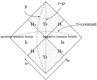
Refer to caption
Figure 3: The Penrose diagram for the induced geometry of the brane corresponding to the situation in Fig. 2. The dashed curve denotes the surface $p$ connecting the two branes.

Each $\tau={\rm constant}$ hypersurface has an Einstein-Rosen bridge around $r=\rho_{*}$. Thus, both the bulk and the brane have non-trivial topology (simply connected but with non-vanishing second Betti number), which represents the creation of a sort of bubble. However it is not possible to traverse from one side to the other: Once $T_{P}$ is entired, it is impossible to leave. Thus, the region $T_{P}$ is a kind of black hole, though it is very different from what we know of black holes. In particular, the total gravitational energy vanishes, which indicates that the vacuum in the RS1 model might decay by creating RS bubbles semi-classically, as we will discuss in the next section. This strange structure results from the fact that there is an effective negative energy distribution on the brane, which is due to the electric part of the five-dimensional Weyl tensor.[14]

As mensioned above, in the RS1 model, the RS vacuum might decay through the semi-classical creation of the RS bubbles. The creation of a bubble implies a connection of two branes through a topology-changing process of the bulk and the brane. To be a good model of the universe, there should be a stabilization against this kind of instability in the RS1 model. In the next section we estimate the decay probability to an RS bubble in the RS1 model.

3 Quantum creation of the Randall-Sundrum bubble

3.1 Decay rate

We now discuss the decay of the RS vacuum to RS bubble spacetime. The corresponding Euclidean solution is obtained by the Wick rotation $\tau\to i\tau_{E}+\pi/2$ of the metric of Eq. (4):

$\displaystyle g$ $\displaystyle=$ $\displaystyle\Bigl{[}\frac{1-(\rho_{*}/ar)^{2}}{1+(\rho_{*}/ar)^{2}}\Bigr{]}^{2}dy^{2}+a^{2}\Bigl{[}1+\Bigl{(}\frac{\rho_{*}}{ar}\Bigr{)}^{2}\Bigr{]}^{2}\Bigl{(}dr^{2}+r^{2}d\Omega_{3}^{2}\Bigr{)},$ (16)

where $d\Omega_{3}^{2}=d\tau_{E}^{2}+{\rm sin}^{2}\tau_{E}d\Omega_{2}^{2}$ is the standard metric of $S^{3}$.

From this point we estimate the nucleation probability of an RS bubble. Since we are interested in the transition rate of the RS vacuum to an RS bubble, we can use the following formula for the decay probability:[19]

$\displaystyle P\sim e^{-(S_{E}-S_{E}^{(0)})}=:e^{-[S_{E}]},$ (17)

where $S_{E}$ and $S_{E}^{(0)}$ are the Euclidean action of the RS bubble and the RS vacuum, respectively. The Euclidean action $S_{E}^{(0)}$ is evaluated in the RS vacuum with the metric

$\displaystyle g$ $\displaystyle=$ $\displaystyle dy^{2}+a^{2}\left(dr^{2}+r^{2}d\Omega_{3}{}^{2}\right).$ (18)

Two 3-branes are located at $y=0$ and $y_{0}$, as shown in Fig. 2. Since both $S_{E}$ and $S_{E}^{(0)}$ diverge, we introduce a cutoff at $r=r_{c}$ such that $S_{E}-S_{E}^{(0)}$ is well-defined in the limit $r_{c}\to+\infty$.

The Euclidean action of the system is given by

$\displaystyle S_{E}=S_{\rm bulk}+S_{\rm brane}+S_{\infty}+S_{p},$ (19)

where

$\displaystyle S_{\rm bulk}$ $\displaystyle=$ $\displaystyle\int_{M}\sqrt{g}\left(\Lambda-\frac{1}{2}R\right)d^{5}x,$ (20)
$\displaystyle S_{\rm brane}$ $\displaystyle=$ $\displaystyle\int_{B}\sqrt{{}^{(4)}g}\frac{\lambda_{+}}{2}d^{4}x-\int_{B}\sqrt{{}^{(4)}g}Kd^{4}x$ (21)
$\displaystyle+\int_{\tilde{B}}\sqrt{{}^{(4)}g}\frac{\lambda_{-}}{2}d^{4}x-\int_{\tilde{B}}\sqrt{{}^{(4)}g}Kd^{4}x,$
$\displaystyle S_{\infty}$ $\displaystyle=$ $\displaystyle-\int_{r=r_{c}}\sqrt{{}^{(4)}g}Kd^{4}x,$ (22)
$\displaystyle S_{p}$ $\displaystyle=$ $\displaystyle-\int_{p}\sqrt{{}^{(4)}g}Kd^{4}x.$ (23)

Here, the positive and negative tension branes are denoted by $B$ and $\tilde{B}$, respectively, $\lambda_{\pm}=\pm 6/\ell$ is the tension of each brane, $\Lambda=-6/\ell^{2}$ is the bulk cosmological constant, and $M$ is the bulk with the cutoff $r=r_{c}$. The quantity $S_{p}$ is the contribution from the edge $p$, which is the surface of intersection of $B$ and $\tilde{B}$. Since there is a deficit angle, the introduction of $S_{p}$ corresponds to that of a string-like defect at the intersection. 222 There is an ambiguity with regard to how one treats this term. This will depend on the microprocesses when two branes collide. We consider a simple case and leave this problem for future investigations.

From the Einstein equation and the junction condition under $Z_{2}$ symmetry,

$\displaystyle S_{\rm bulk}=\frac{4}{\ell^{2}}Vol_{5}(M)$ (24)

and

$\displaystyle S_{\rm branes}$ $\displaystyle=$ $\displaystyle-\frac{1}{\ell}\left[Vol_{4}(B)-Vol_{4}(\tilde{B})\right]$ (25)

are obtained, where $Vol_{n}$ denotes the $n$-dimensional volume.

3.2 Euclidean action of the RS vacuum

For the RS vacuum the volumes of the bulk and the branes become

$\displaystyle Vol_{5}(M)=2\pi^{2}\int^{y_{0}}_{0}dy\int^{r_{c}}_{0}dra^{4}r^{3}=\frac{\pi^{2}}{8}\left(1-e^{-4y_{0}/\ell}\right)\ell r_{c}^{4},$ (26)
$\displaystyle Vol_{4}(B)=2\pi^{2}\int^{r_{c}}_{0}drr^{3}a^{4}=\frac{\pi^{2}}{2}r_{c}^{4},$ (27)
$\displaystyle Vol_{4}(\tilde{B})=2\pi^{2}\int^{r_{c}}_{0}drr^{3}a^{4}=\frac{\pi^{2}}{2}r_{c}^{4}e^{-4y_{0}/\ell}.$ (28)

Each contribution to the action therefore becomes

$\displaystyle S_{\rm bulk}^{(0)}$ $\displaystyle=$ $\displaystyle\frac{1}{2}\pi^{2}\left(1-e^{-4y_{0}/\ell}\right)\frac{r_{c}^{4}}{\ell},$ (29)
$\displaystyle S_{\rm brane}^{(0)}$ $\displaystyle=$ $\displaystyle-\frac{1}{2}\pi^{2}\left(1-e^{-4y_{0}/\ell}\right)\frac{r_{c}^{4}}{\ell},$ (30)
$\displaystyle S_{\infty}^{(0)}$ $\displaystyle=$ $\displaystyle-3\pi^{2}\left(1-e^{-2y_{0}/\ell}\right)\ell r_{c}^{2}.$ (31)

Since there are no edges in the RS vacuum, $S_{p}^{(0)}=0$. Thus the total Euclidean action of the RS vacuum is given by

$\displaystyle S_{E}^{(0)}=S^{(0)}_{\infty}=-3\pi^{2}\ell r_{c}^{2}\left(1-e^{-2y_{0}/\ell}\right).$ (32)

Note that the contributions from the bulk and the brane exactly cancel, due to the exact balance of the bulk cosmological constant and the tension of the flat branes:

$\displaystyle S_{\rm bulk}^{(0)}+S_{\rm brane}^{(0)}=0.$ (33)

3.3 The Euclidean action of an RS bubble

For the RS bubble space-time, the volumes of the bulk and branes are

$\displaystyle Vol_{5}(M)$ $\displaystyle=$ $\displaystyle 2\pi^{2}\int^{y_{0}}_{0}dy\int^{r_{c}}_{r_{0}(y)}dra^{4}r^{3}\Bigl{[}1-\Bigl{(}\frac{\rho_{*}}{ar}\Bigr{)}^{2}\Bigr{]}\biggl{[}1+\Bigl{(}\frac{\rho_{*}}{ar}\Bigr{)}^{2}\biggr{]}^{3}$ (34)
$\displaystyle=$ $\displaystyle\pi^{2}\rho_{*}^{4}\ell\biggl{[}\frac{1}{8}\Bigl{(}\frac{\rho_{*}}{r_{c}}\Bigr{)}^{4}(a_{0}^{-4}-1)+\Bigl{(}\frac{\rho_{*}}{r_{c}}\Bigr{)}^{2}(a_{0}^{-2}-1)$
$\displaystyle-\Bigl{(}\frac{r_{c}}{\rho_{*}}\Bigr{)}^{2}(a_{0}^{2}-1)-\frac{1}{8}\Bigl{(}\frac{r_{c}}{\rho_{*}}\Bigr{)}^{4}(a_{0}^{4}-1)\biggr{]}$
$\displaystyle-\pi^{2}\rho_{*}^{4}\int^{y_{0}}_{0}dy\biggl{[}\frac{1}{2}\left(\frac{ar_{0}(y)}{\rho_{*}}\right)^{-4}+2\left(\frac{ar_{0}(y)}{\rho_{*}}\right)^{-2}$
$\displaystyle+2\left(\frac{ar_{0}(y)}{\rho_{*}}\right)^{2}+\frac{1}{2}\left(\frac{ar_{0}(y)}{\rho_{*}}\right)^{4}\biggr{]},$
$\displaystyle Vol_{4}(B)$ $\displaystyle=$ $\displaystyle 2\pi^{2}\int_{r_{0}(0)}^{r_{c}}r^{3}\left[1+\left(\frac{\rho_{*}}{r}\right)^{2}\right]^{4}dr$ (35)
$\displaystyle=$ $\displaystyle\pi^{2}\rho_{*}^{4}\left[\frac{1}{2}\left(\frac{r_{c}}{\rho_{*}}\right)^{4}\right.+4\left(\frac{r_{c}}{\rho_{*}}\right)^{2}+12\ln\left(\frac{r_{c}}{\rho_{*}}\right)-4\left(\frac{r_{c}}{\rho_{*}}\right)^{-2}$
$\displaystyle-\frac{1}{2}\left(\frac{r_{c}}{\rho_{*}}\right)^{-4}-\frac{1}{2}\left(\frac{r_{0}(0)}{\rho_{*}}\right)^{4}{}-4\left(\frac{r_{0}(0)}{\rho_{*}}\right)^{2}-12\ln\left(\frac{r_{0}(0)}{\rho_{*}}\right)$
$\displaystyle\left.+4\left(\frac{r_{0}(0)}{\rho_{*}}\right)^{-2}+\frac{1}{2}\left(\frac{r_{0}(0)}{\rho_{*}}\right)^{-4}\right],$
$\displaystyle Vol_{4}(\tilde{B})$ $\displaystyle=$ $\displaystyle 2\pi^{2}\int_{\rho_{*}^{2}/a_{0}r_{0}(0)}^{r_{c}}a_{0}{}^{4}r^{3}\left[1+\left(\frac{\rho_{*}}{a_{0}r}\right)^{2}\right]^{4}dr$ (36)
$\displaystyle=$ $\displaystyle\pi^{2}\rho_{*}^{4}\left[\frac{1}{2}\left(\frac{a_{0}r_{c}}{\rho_{*}}\right)^{4}\right.+4\left(\frac{a_{0}r_{c}}{\rho_{*}}\right)^{2}+12\ln\left(\frac{a_{0}r_{c}}{\rho_{*}}\right)-4\left(\frac{a_{0}r_{c}}{\rho_{*}}\right)^{-2}$
$\displaystyle-\frac{1}{2}\left(\frac{a_{0}r_{c}}{\rho_{*}}\right)^{-4}-\frac{1}{2}\left(\frac{r_{0}(0)}{\rho_{*}}\right)^{4}{}-4\left(\frac{r_{0}(0)}{\rho_{*}}\right)^{2}-12\ln\left(\frac{r_{0}(0)}{\rho_{*}}\right)$
$\displaystyle\left.+4\left(\frac{r_{0}(0)}{\rho_{*}}\right)^{-2}+\frac{1}{2}\left(\frac{r_{0}(0)}{\rho_{*}}\right)^{-4}\right],$

where $a_{0}=e^{-y_{0}/\ell}$, and $r_{0}(y)$ is implicitly defined as the larger solution of the equations

$\displaystyle\frac{y_{0}-y}{2}$ $\displaystyle=$ $\displaystyle\frac{1}{\ell}\int^{R}_{R_{*}}dRR\left[1-\left(\frac{2\rho_{*}}{R}\right)^{2}+\left(\frac{R}{\ell}\right)^{2}\right]^{-1}\left[1-\left(\frac{2\rho_{*}}{R}\right)^{2}\right]^{-1/2},$ (37)
$\displaystyle R$ $\displaystyle=$ $\displaystyle a(y)r_{0}(y)\left[1+\left(\frac{\rho_{*}}{a(y)r_{0}(y)}\right)^{2}\right].$ (38)

As seen below, we need a numerical computation to determine $r_{0}(y)$ in general.

Though both $S_{\rm bulk}$ and $S_{\rm brane}$ are unbounded, the divergent terms again cancel, and we obtain

$\displaystyle S_{\rm bulk}+S_{\rm brane}$ $\displaystyle=$ $\displaystyle\frac{\pi^{2}\rho_{*}^{4}}{\ell}\left\{\left(\frac{r_{0}(0)}{\rho_{*}}\right)^{4}+8\left(\frac{r_{0}(0)}{\rho_{*}}\right)^{2}+24\ln\frac{r_{0}(0)}{\rho_{*}}-8\left(\frac{r_{0}(0)}{\rho_{*}}\right)^{-2}\right.$ (39)
$\displaystyle{}-\left(\frac{r_{0}(0)}{\rho_{*}}\right)^{-4}-12\frac{y_{0}}{\ell}-\frac{1}{\ell}\int_{0}^{y_{0}}\left[2\left(\frac{ar_{0}}{\rho_{*}}\right)^{4}+8\left(\frac{ar_{0}}{\rho_{*}}\right)^{2}\right.$
$\displaystyle\left.\left.+8\left(\frac{ar_{0}}{\rho_{*}}\right)^{-2}+2\left(\frac{ar_{0}}{\rho_{*}}\right)^{-4}\right]dy\right\}$
$\displaystyle=$ $\displaystyle\frac{\pi^{2}\rho_{*}^{4}}{\ell}\left\{16\frac{\rho_{p}^{4}}{\rho_{*}^{4}}\left(1+\frac{3\rho_{*}^{2}}{2\rho_{p}^{2}}\right)\sqrt{1-\frac{\rho_{*}^{2}}{\rho_{p}^{2}}}+24\ln\frac{\rho_{p}}{\rho_{*}}\left(1+\sqrt{1-\frac{\rho_{*}^{2}}{\rho_{p}^{2}}}\right)\right.$
$\displaystyle-12\frac{y_{0}}{\ell}-\frac{1}{\ell}\int_{0}^{y_{0}}\left[2\left(\frac{ar_{0}}{\rho_{*}}\right)^{4}+8\left(\frac{ar_{0}}{\rho_{*}}\right)^{2}\right.$
$\displaystyle\left.\left.+8\left(\frac{ar_{0}}{\rho_{*}}\right)^{-2}+2\left(\frac{ar_{0}}{\rho_{*}}\right)^{-4}\right]dy\right\},$

where

$$\rho_{p}:=\frac{r_{0}(0)}{2}\left[1+\left(\frac{\rho_{*}}{r_{0}(0)}\right)^{2}\right]$$ (40)

denotes half the volume radius at $p$. As seen below $S_{\rm bulk}+S_{\rm brane}$ is much smaller than $S_{p}$.

The $r=r_{c}$ term $S_{\infty}$ of the Euclidean action is estimated as

$$S_{\infty}=-3\pi^{2}r_{c}^{2}\ell(1-e^{-2y_{0}/\ell})+4\pi^{2}\rho_{*}^{2}y_{0}.$$ (41)

This shows that the contribution from the boundary is also finite: $[S_{\infty}]=S_{\infty}-S_{\infty}^{(0)}=4\pi^{2}\rho_{*}^{2}y_{0}<+\infty$.

Following Ref.  [20], $S_{p}$ is evaluated as

$$S_{p}=16\pi^{2}\rho_{p}^{3}\Delta\phi_{p},$$ (42)

where $\Delta\phi_{p}$ is the exterior angle in the ($R$,$\Theta$)-plane at $p$. The exterior angle $\Delta\phi_{p}$ is evaluated as

$\displaystyle\Delta\phi_{p}$ $\displaystyle=$ $\displaystyle{\rm cos}^{-1}(-g_{\mu\nu}n^{\mu}_{+}n^{\nu}_{-})$ (43)
$\displaystyle=$ $\displaystyle\cos^{-1}\left[\frac{4\left(\rho_{p}/\ell\right)^{2}+\left(\rho_{*}/\rho_{p}\right)^{2}-1}{4\left(\rho_{p}/\ell\right)^{2}-\left(\rho_{*}/\rho_{p}\right)^{2}+1}\right],$

where $n_{\pm}$ are the unit normal vectors of the $(\pm)$-branes at $p$ given by

$$n_{\pm}=\sqrt{1-\frac{\rho_{*}^{2}}{\rho_{p}^{2}}}\left[-\frac{1}{F(2\rho_{p})}\partial_{\Theta}\pm\frac{2\rho_{p}}{\ell\sqrt{1-\rho_{*}^{2}/\rho_{p}^{2}}}\partial_{R}\right].$$ (44)

Thus we obtain

$$S_{p}=16\pi^{2}\rho_{p}^{3}\cos^{-1}\left[\frac{4\left(\rho_{p}/\ell\right)^{2}+\left(\rho_{*}/\rho_{p}\right)^{2}-1}{4\left(\rho_{p}/\ell\right)^{2}-\left(\rho_{*}/\rho_{p}\right)^{2}+1}\right].$$ (45)

Gathering Eqs. (39) (41) and (45), we obtain the total action, Eq. (19).

3.4 Estimation of the decay rate

We are now ready to evaluate the transition probability from the RS vacuum to the RS bubble,

$$P\sim\exp\left(-[S_{E}]\right).$$ (46)

In general, we need a numerical computation to evaluate $[S_{E}]$. The numerical results are given in Figs. 4 and 5. It is seen that the dominant contribution to $[S_{E}]$ comes from $S_{p}$, while the contribution from $S_{\rm brane}+S_{\rm bulk}$ is relatively small. In addition we can see from Fig. 6 that the $\rho_{*}$ dependence of $S_{p}$ is mainly governed by $R_{p}$. The contribution $S_{p}$ is a non-monotonic function at small $R_{*}$. The volume effect of RS bubble reduces the decay rate for relatively large $\rho_{*}$. In any case, an RS bubble with small $\rho_{*}$ and small $y_{0}$ will be nucleated easily. Once created, a bubble quickly expands at nearly the speed of light and eventually occupies the entire universe. For $y_{0}\sim 40\ell$, however, we can see from Fig. 5 that the transition amplitude is significantly suppressed.

Refer to caption
Figure 4: The Euclidean action between the RS vacuum and the bubble for $y_{0}=\ell=1$. Here “bulk+brane”, “$r$ cutoff”, “edge” and “total” correspond to $S_{\rm bulk}+S_{\rm brane}$, $S_{\infty}$, $S_{p}$ and $[S_{E}]$, respectively.
Refer to caption
Figure 5: $[S_{E}]$ for $\ell=1$ and $y_{0}=0.5,1,5$. In all cases $S_{p}$ dominates.
Refer to caption
Figure 6: $R_{p}$, $r_{0}(0)$ and $\Delta\phi_{p}$ for $\ell=1$. $R_{p}$ determines the behavior of $S_{p}$.

Finally, we give some useful analytic expressions using some limiting conditions. When $R_{*}=0$, the function $r_{0}(y)$ is given by

$$a(y)r_{0}(y)=\ell\sqrt{e^{(y_{0}-y)/\ell}-1},$$ (47)

and $\rho_{p}$ becomes

$$\rho_{p}=\frac{\ell}{2}\sqrt{e^{y_{0}/\ell}-1}.$$ (48)

Then, we obtain

$\displaystyle S_{\rm bulk}+S_{\rm brane}=2\pi^{2}\ell^{3}\left[e^{y_{0}/\ell}-1-\frac{y_{0}}{\ell}\right],$ (49)
$\displaystyle S_{\infty}-S^{(0)}_{\infty}=0,$ (50)
$\displaystyle S_{p}=16\pi^{2}\rho_{p}^{3}\cos^{-1}\left[\frac{4\left(\rho_{p}/\ell\right)^{2}-1}{4\left(\rho_{p}/\ell\right)^{2}+1}\right].$ (51)

With the further limiting condition $y_{0}/\ell\ll 1$, the difference from the Euclidean action becomes

$$[S_{E}]\simeq S_{p}\simeq\frac{\pi^{2}\ell^{3}}{G_{5}}\Bigl{(}\frac{y_{0}}{\ell}\Bigr{)}^{3/2},$$ (52)

where $G_{5}$ has been recovered.

When $R_{*}/\ell\gg 1$ on the other hand, we have $1-(R_{*}/R)^{2}\ll(R/\ell)^{2}$, so that the coordinate transformation can be explicitly carried out in this case. Then, $r_{0}(y)$ is simply given by

$$a(y)r_{0}(y)\simeq\rho_{*}\exp\left(\pm\frac{y_{1}-y}{2\ell}\right),$$ (53)

where the upper sign is for the bulk and the positive tension brane, and the lower sign is for the negative tension brane. In this limit, we can see that the term $S_{\rm bulk}+S_{\rm brane}$ has only a small contribution. In addition, we have $[S_{\infty}]\simeq-6\pi^{2}\rho_{*}^{2}\ell(1-e^{-2y_{0}/\ell})+4\pi^{2}\rho_{*}^{2}y_{0}$ and $S_{p}\simeq 8\pi^{2}\rho_{*}^{2}\ell\sinh(y_{0}/\ell)$. Then $[S_{E}]$ becomes

$\displaystyle[S_{E}]$ $\displaystyle\simeq$ $\displaystyle[S_{\infty}]+S_{p}$ (54)
$\displaystyle\simeq$ $\displaystyle-6\pi^{2}\rho_{*}^{2}\ell(1-e^{-2y_{0}/\ell})+4\pi^{2}\rho_{*}^{2}y_{0}$
$\displaystyle+8\pi^{2}\rho_{*}^{2}\ell\sinh(y_{0}/\ell).$

Note that the bulk term and the brane term of the Euclidean action cancel out. With the further condition $y_{0}/\ell\ll 1$, the difference of the Euclidean action is

$\displaystyle[S_{E}]\simeq 48\pi^{2}\frac{\rho_{*}^{2}y_{0}^{2}}{G_{5}\ell},$ (55)

while for $y_{0}\sim\ell$, we have

$\displaystyle[S_{E}]\simeq 8\pi^{2}\frac{\rho_{*}^{2}\ell}{G_{5}}.$ (56)

If we are interested in the hierarchy problem, we can set $y_{0}\sim 40\ell$[2] in Eq. (54). Then we obtain

$\displaystyle[S_{E}]\simeq 10^{19}\times\Bigl{(}\frac{\rho_{*}^{2}\ell}{G_{5}}\Bigr{)}.$ (57)

Except for the large numerical prefactor, the dependence of $[S_{E}]$ on the physical parameters $\rho_{*}$ and $\ell$ is found in a previous paper. [14] It should be noted that we cannot set $\rho_{*}=0$ in Eq. (57) because we are assuming $\rho_{*}/\ell\gg 1$.

4 Summary

Let us summarize our study. We have investigated the instanton solution that describes the decay of the RS vacuum into an RS bubble. The decay probability is numerically estimated. We also derived an analytic formula for the decay probability into large RS bubbles. We found that the RS vacuum (RS1 model) is unstable in general. We also found that decay into a small RS bubble is favored over decay into a large RS bubble, as be expected. However, the transition rate is suppressed when two branes are sufficiently separated as is assumed in the context of the hierarchy problem.

Our result brings to light a problem concerning the stability of the brane world. The entire space will be quickly occupied by RS bubbles. This is, however, a topology-changing process, so that this instability might be forbidden by the introduction of spinor fields. A supersymmetry might also serve as a stabilizer.

Acknowledgements

HO would like to thank K. Sato for his continuous encouragement. TS’s work is partially supported by the Yamada Science Foundation.

References

  • [1] P. Horava and E. Witten, Nucl. Phys. B460(1996),506; B475 (1996), 94.
  • [2] L. Randall and R. Sundrum, Phys. Rev. Lett. 83(1999), 3370.
  • [3] L. Randall and R. Sundrum, Phys. Rev. Lett. 83(1999), 4690
  • [4] J. Garriga and T. Tanaka, Phys. Rev. Lett. 84 (2000), 2778;
    S. B. Giddings, E. Katz, and L. Randall, JHEP 0003(2000), 023.
  • [5] T. Shiromizu, K. Maeda, M. Sasaki, Phys. Rev. D62 (2000), 024012;
    M. Sasaki, T. Shiromizu and K. Maeda, Phys. Rev. D62, (2000), 024008.
  • [6] P. Binétruy, C. Deffayet, U. Ellwanger and D. Langlois, Phys. Lett. B477(2000), 285.
    P. Kraus, JHEP 9912(1999), 011.
    D. Ida, JHEP 0009(2000), 014.
    S. Mukohyama, Phys. Lett. B473 (2000), 241.
    S. Mukohyama, T. Shiromizu and K. Maeda, Phys. Rev. D62 (2000), 024028.
  • [7] S. S. Gubser, Phys. Rev. D63 (2001), 084017.
    M.J. Duff and J. T. Liu, Phys. Rev. Lett. 85 (2000), 2052.
    M. Perez-Victoria, hep-th/0105048.
    T. Shiromizu and D. Ida, Phy. Rev. D64 (2001), 044015.
    A. Hebecker and J. March-Russell, hep-ph/0103214.
    S. W. Hawking, T. Hertog and H. S. Reall, Phys. Rev. D62(2000), 043501.
    L. Anchordoqui, C. Nunez and K. Olsen, JHEP 0010(2000), 050.
    S. Nojiri, S.D. Odintsov and S. Zerbini, Phys. Rev. D62 (2000), 064006.
    S. Nojiri and S.D. Odintsov, Phys. Lett. B484 (2000), 119.
  • [8] T. Tanaka and X. Montes, Nucl. Phys. B582(2000), 259.
  • [9] W. D. Goldberger and M. B. Wise, Phys. Rev. Lett. 83 (1999), 4922.
  • [10] E. Witten, Nucl. Phys. B195(1982), 481.
  • [11] D. Brill and H. Pfisher, Phys. Lett. B228(1989), 359.
    D. Brill and G. T. Horowitz, Phys. Lett. B262(1991), 437.
  • [12] H. Shinkai and T. Shiromizu, Phys. Rev. D62(2000), 024010.
  • [13] M. Fabinger and P. Horava, Nucl. Phys. B580(2000), 243.
  • [14] D. Ida, T. Shiromizu and H. Ochiai, Phys. Rev. D65 (2002) 023504.
  • [15] R. Gregory and A. Padilla, hep-th/0104262; hep-th/0107108.
  • [16] T. Shiromizu, D. Ida and T. Torii, JHEP 0111 (2001) 010..
  • [17] G. C. MacVittie, Month. Not. Roy. Astron. Soc. 93(1933), 325.
    M. Kihara and H. Nariai, Prog. Theor. Phys. 65(1981), 1613.
  • [18] A. Einstein and N. Rosen, Phys. Rev. 48(1935), 73.
  • [19] R. Bousso and A. Chamblin, Phys. Rev. D59(1999), 084004.
    U. Gen and M. Sasaki, Phys. Rev. D61(2000), 103508.
  • [20] G. Hayward, Phys. Rev. D47(1993), 3275.