HUTP-01/A053

UTTG-16-01

hep-th/0111068

A Mysterious Duality
Amer Iqbal${}^{~{}1}$, Andrew Neitzke${}^{~{}2}$ and Cumrun Vafa${}^{~{}3}$

¹Theory Group, Department of Physics

University of Texas at Austin,

Austin, TX 78712, U.S.A.

²Department of Mathematics

Harvard University

Cambridge, MA 02138, U.S.A.

³ Jefferson Physical Laboratory,

Harvard University

Cambridge, MA 02138, U.S.A.

We establish a correspondence between toroidal compactifications of M-theory and del Pezzo surfaces. M-theory on $T^{k}$ corresponds to ${\mathbb{P}}^{2}$ blown up at $k$ generic points; Type IIB corresponds to ${\mathbb{P}}^{1}\times{\mathbb{P}}^{1}$. The moduli of compactifications of M-theory on rectangular tori are mapped to Kähler moduli of del Pezzo surfaces. The U-duality group of M-theory corresponds to a group of classical symmetries of the del Pezzo represented by global diffeomorphisms. The $\frac{1}{2}$-BPS brane charges of M-theory correspond to spheres in the del Pezzo, and their tension to the exponentiated volume of the corresponding spheres. The electric/magnetic pairing of branes is determined by the condition that the union of the corresponding spheres represent the anticanonical class of the del Pezzo. The condition that a pair of $\frac{1}{2}$-BPS states form a bound state is mapped to a condition on the intersection of the corresponding spheres. We present some speculations about the meaning of this duality.

1 Introduction

The discovery of duality symmetries in string theory has led to spectacular progress in our understanding of non-perturbative aspects of the theory. However, we still do not have a deep understanding of the meaning of these symmetries. Indeed, we find ourselves in the strange situation that the quantum corrected physics has more symmetries than the classical strings had any right to expect!

A clear appreciation of symmetry principles is a sacred principle of physics. Given any physical system, we should formulate the theory in a way that makes all of the symmetries manifest. But despite many years of work on a non-perturbative definition of string theory, we are no closer to making duality symmetries manifest than when the dualities were first discovered!

We would like to have a formulation of string theory in which all of the duality symmetries are classically visible. The aim of this paper is to develop a mysterious duality which points to the existence of such a formulation.

It was noted in [1] that there is a classical geometric system which shares all the U-duality symmetries of M-theory compactified on rectangular tori. The relevant geometric objects are del Pezzo surfaces, which are complex 2-dimensional Kähler manifolds with $c_{1}>0$. In this correspondence, M-theory in 11 dimensions is mapped to ${\mathbb{P}}^{2}$, and subsequent compactifications of M-theory on rectangular tori $T^{k}$ are mapped to ${\mathbb{P}}^{2}$ blown up at $k$ generic points (i.e. a manifold in which $k$ generic points on ${\mathbb{P}}^{2}$ are replaced with ${\mathbb{P}}^{1}$’s), which is a del Pezzo surface denoted $\mathbb{B}_{k}$. Type IIB is mapped to ${\mathbb{P}}^{1}\times{\mathbb{P}}^{1}$, which can be viewed as a blow down of $\mathbb{B}_{2}$. The U-duality group of M-theory on $T^{k}$, which for rectangular compactifications with no $C$-field vevs is given by the Weyl group of $E_{k}$ (with a suitable definition for small $k$), is mapped to a subgroup of the global diffeomorphisms of the del Pezzo. For example, the $S$-duality of type IIB in 10 dimensions is realized as the exchange of the two ${\mathbb{P}}^{1}$’s in ${\mathbb{P}}^{1}\times{\mathbb{P}}^{1}$.

We will show in this paper that one can take this idea quite far, constructing a precise dictionary relating the two sides. In particular, the $\frac{1}{2}$-BPS $p$-branes of M-theory will be mapped to rational curves on the del Pezzo. Furthermore, we find a map which relates the moduli of the (extended) Kähler metric on $\mathbb{B}_{k}$, which is determined by $k+1$ real parameters (one for the overall size of the original ${\mathbb{P}}^{2}$ and $k$ for the volumes of the blown-up ${\mathbb{P}}^{1}$’s) with the $k+1$ moduli of M-theory on $T^{k}$ ($k$ moduli for the compactification radii and one for the Planck scale). The moduli space of Kähler classes also carries an action of a group of global diffeomorphisms of the del Pezzo surface, which exchange the various embedded 2-spheres; as noted above, this group is isomorphic to the Weyl group of $E_{k}$. Moreover, this symmetry action is compatible with the identification of the moduli on the two sides. The map relates the tension of a $\frac{1}{2}$-BPS state with the exponential of the volume of the corresponding ${\mathbb{P}}^{1}$. In addition, electric/magnetic duality and the condition for a pair of branes to form a bound state admit a nice geometric interpretation on the del Pezzo side.

Some aspects of the dictionary we construct are listed in the table below:

del Pezzo $\mathbb{B}_{k}$	M-theory on $T^{k}$
Element of $H^{2}(\mathbb{B}_{k},{\mathbb{R}})$	Point in moduli space of M-theory on $T^{k}$
Global diffeomorphisms	U-duality group
preserving the canonical class $K$
2-sphere ${\mathcal{C}}$ with volume $V_{\cal C}$ and	$\frac{1}{2}$-BPS $p$-brane state with tension $2\pi\exp V_{C}$
degree $p+1$
Volume $V_{K}$ of canonical class	Compactified Planck length, $\widetilde{l_{p}}^{9-k}=\exp V_{K}$
Volume $V_{H}$ of hyperplane class	11-dimensional Planck length, $l_{p}^{-3}=\exp V_{H}$
Volume $V_{E}$ of exceptional curve	Radius $2\pi R=\exp-V_{E}$
$H$, line in ${\mathbb{P}}^{2}$	M2-brane
2$H$, conic in ${\mathbb{P}}^{2}$	M5-brane
2-spheres ${\mathcal{C}}_{1}$, ${\mathcal{C}}_{2}$ with ${\mathcal{C}}_{1}+{\mathcal{C}}_{2}=-K$	Electric-magnetic dual objects

Here $H$ denotes the class of a hyperplane (a complex line) in ${\mathbb{P}}^{2}$, and $K$ denotes the “canonical class,” a 2-cycle class which is dual to the negative of the first Chern class of the del Pezzo.

The organization of this paper is as follows: In Section 2 we review some relevant geometric aspects of del Pezzo surfaces. In Section 3 we present the map between the two sides. In Section 4 we discuss some speculations as to the meaning of this duality and raise some natural questions.

2 Del Pezzo surfaces

2.1 Basic properties

The term “del Pezzo surface” refers to any manifold of complex dimension $2$ such that the first Chern class is positive [2]. These surfaces admit metrics of positive scalar curvature. They may be classified as follows: either take ${\mathbb{P}}^{2}$ and blow up $k\leq 8$ generic points, or take ${\mathbb{P}}^{1}\times{\mathbb{P}}^{1}$ and blow up $k\leq 7$ generic points. We call the resulting del Pezzos $\mathbb{B}_{k}$ and ${\mathbb{F}}^{k}$ respectively. In fact $\mathbb{B}_{k+1}\simeq{\mathbb{F}}^{k}$ for $k\geq 1$, so it is enough to consider only $\mathbb{B}_{k}$ and ${\mathbb{P}}^{1}\times{\mathbb{P}}^{1}$.

Now let us describe the homology of del Pezzo surfaces, beginning with ${\mathbb{P}}^{2}$. Since ${\mathbb{P}}^{2}$ is simply connected the only interesting homology will be in dimension 2; in fact $H_{2}({\mathbb{P}}^{2},{\mathbb{Z}})$ is simply ${\mathbb{Z}}$, generated by the class of a line, which we write $H$. When we blow up a point we replace it with a ${\mathbb{P}}^{1}$ (a 2-sphere), which gives a new generator in $H_{2}(\mathbb{B}_{k},{\mathbb{Z}})$ for each of the $k$ points we blow up. Thus $\mbox{dim}\ H_{2}(\mathbb{B}_{k},{\mathbb{R}})=k+1$; a natural basis to choose is $\{H,E_{1},\dots,E_{k}\}$, where the $E_{a}$ are the “exceptional curves” obtained by blow-ups and $H$ represents the pullback of the generator of $H_{2}({\mathbb{P}}^{2},{\mathbb{Z}})$ under the projection

$$\pi\,:\,\mathbb{B}_{k}\to\mathbb{B}_{0}=\mathbb{P}^{2}$$ (1)

which simply collapses each exceptional curve $E_{a}$ to the corresponding point $p_{a}\in\mathbb{P}^{2}$ which was blown up. The intersection numbers are given by [3]

$$H\cdot H=1\,,\,\,H\cdot E_{a}=0\,,\,\,E_{a}\cdot E_{b}=-\delta_{ab}\,,\,a,b=1,\cdots,k\,.$$ (2)

For $\mathbb{F}^{k-1}$, $\mathrm{dim}\ H_{2}(\mathbb{F}^{k-1},{\mathbb{R}})=k+1$ and the natural basis is given by $\{l_{1},l_{2},e_{1},\dots,e_{k-1}\}$ (the $l_{i}$ come from ${\mathbb{P}}^{1}\times{\mathbb{P}}^{1}$ and the $e_{j}$ are the blown-up ${\mathbb{P}}^{1}$’s) satisfying

$$l_{i}\cdot l_{j}=1-\delta_{ij}\,,\,\,l_{i}\cdot e_{a}=0\,,\,\,e_{a}\cdot e_{b}=-\delta_{ab}\,,\,\,i,j=1,2\,;\,\,a,b=1,\cdots,k-1\,.$$ (3)

Since $\mathbb{B}_{k}\simeq{\mathbb{F}}^{k+1}$ we can write the two bases just described in terms of one another; the map is given by

$$H \mapsto l_{1}+l_{2}-e_{1}\,,$$ (4)

$$E_{1} \mapsto l_{2}-e_{1}\,,$$

$$E_{2} \mapsto l_{1}-e_{1}\,,$$

$$E_{a+1} \mapsto e_{a}\,,\,\,\,\,a=2,\cdots,k-1\,.$$

The inverse map is then

$$l_{1} \mapsto H-E_{1}\,,$$ (5)

$$l_{2} \mapsto H-E_{2}\,,$$

$$e_{1} \mapsto H-E_{1}-E_{2}\,,$$

$$e_{a} \mapsto E_{a+1}\,,\,\,\,\,a=2,\cdots,k-1\,.$$

The canonical class, defined to be minus the first Chern class of the tangent bundle, will play an important role in our correspondence to M-theory; it is given by

$$K_{\mathbb{B}_{k}}= -c_{1}(\mathbb{B}_{k})=-3H+\sum_{a=1}^{k}E_{a}\,,$$ (6)

$$K_{\mathbb{F}^{k-1}}= -c_{1}(\mathbb{F}^{k-1})=-2l_{1}-2l_{2}+\sum_{a=1}^{k-1}e_{a}\,,$$ (7)

where $c_{1}(X)$ is the first Chern class of $X$. Incidentally, from (6) we see directly that the condition of positive first Chern class is not satisfied for $\mathbb{B}_{k}$ or $\mathbb{F}^{k-1}$ with $k>8$, since

$$c_{1}^{2}(X)=K_{X}^{2}=9-k\,\,\,\,\mbox{for}\,\,\,X=\mathbb{B}_{k}\mathrm{\ or\ }X=\mathbb{F}^{k-1}\,.$$ (8)

We denote by $d_{{\cal C}}$ the degree of a class ${\cal C}\in H_{2}(\mathbb{B}_{k})$, which by definition is the intersection of ${\cal C}$ with the anticanonical class, i.e.

$$d_{{\cal C}}:=-{\cal C}\cdot K_{\mathbb{B}_{k}}\,.$$ (9)

The terminology “degree” is explained by the fact that one can use the anticanonical class to give a map of $\mathbb{B}_{k}$ into projective space, and if $\cal C$ is represented by a holomorphic curve then its image will have degree precisely $d_{{\cal C}}$.

If the class ${\cal C}\in H_{2}(\mathbb{B}_{k})$ is realized as a genus $g$ curve then we have an important relation between its self-intersection and its degree, known as the adjunction formula [4]:

$${\cal C}^{2}=2g-2+d_{{\cal C}}\,.$$ (10)

2.2 $E_{k}$ root lattice

We now review an important relation between del Pezzo surfaces and exceptional Lie algebras. Namely, the lattice $H_{2}(\mathbb{B}_{k},\mathbb{Z})$ endowed with the intersection product has a natural sublattice obtained by restricting to the orthogonal complement of $K_{\mathbb{B}_{k}}$, which turns out to be isomorphic to the root lattice of $E_{k}$. To see this (in case $k\geq 3$ — for $k=1,2$ the story is slightly irregular) a convenient basis for the sublattice is the following, which is also a set of simple roots:

$$\alpha_{i} =E_{i}-E_{i+1}\,,\,\,\,\,i=1,\cdots,k-1\,,$$ (11)

$$\alpha_{k} =H-E_{1}-E_{2}-E_{3}\,.$$

It is easy to see that these classes are orthogonal to the canonical class, and that their intersection numbers are given by

$$K_{\mathbb{B}_{k}}\cdot\alpha_{a}=0\,,\,\,\,\alpha_{a}\cdot\alpha_{b}=-A_{ab}\,,\,\,a,b=1,\cdots,k\,,$$ (12)

where $A_{ab}$ represents the Cartan matrix of the Lie algebra $E_{k}$. The Dynkin diagrams of the Lie algebras $E_{k}$ are shown in Fig. 1.

Figure 1: The Dynkin diagrams of exceptional Lie algebras $E_{k}$.

To each ${\cal C}\in H_{2}(\mathbb{B}_{k},\mathbb{Z})$ we can associate an $E_{k}$ weight vector ${\mathcal{C}}_{\perp}$, obtained by projecting onto the orthogonal complement of $K_{\mathbb{B}_{k}}$. The Dynkin labels of ${\mathcal{C}}_{\perp}$ are given by

$$\lambda_{a}=-{\cal C}\cdot\alpha_{a}\,.$$ (13)

In terms of the weight vector, the self-intersection of ${\cal C}\in H_{2}(\mathbb{B}_{k},\mathbb{Z})$ is given by

$${\cal C}^{2}={\mathcal{C}}_{\perp}^{2}+\frac{d_{{\cal C}}^{2}}{9-k}\,.$$ (14)

Because of the minus sign in (12) we will have ${\mathcal{C}}_{\perp}^{2}\leq 0$. Thus the lattice $H_{2}(\mathbb{B}_{k},\mathbb{Z})$ has signature $(1,k)$,

$$H_{2}(\mathbb{B}_{k},\mathbb{Z})=\langle K_{\mathbb{B}_{k}}\rangle\,\oplus\,\Gamma_{E_{k}}\,.$$ (15)

Here $\Gamma_{E_{k}}$ is the root lattice of $E_{k}$, with the sign of the inner product reversed.

2.3 Weyl group

Next we show that the Weyl group of $E_{k}$ acts naturally on $H_{2}(\mathbb{B}_{k},{\mathbb{R}})$, preserving the intersection form and $K_{\mathbb{B}_{k}}$. Given any $\alpha\in H_{2}(\mathbb{B}_{k},{\mathbb{Z}})$ with $\alpha^{2}=-2$ and $K_{\mathbb{B}_{k}}\cdot\alpha=0$ (a root) we can define a transformation $w_{\alpha}$, which is the reflection in $\alpha$ and hence acts orthogonally:

$$w_{\alpha}:\,{\mathcal{C}}\mapsto{\mathcal{C}}+({\mathcal{C}}\cdot\alpha)\,\alpha\,,\,\,\,{\mathcal{C}}\in H_{2}(\mathbb{B}_{k})\,.$$ (16)

The elements $w_{\alpha}$ corresponding to simple roots have a particularly interesting action on $H_{2}(\mathbb{B}_{k},{\mathbb{R}})$. The simple root $\alpha_{i}=E_{i}-E_{i+1}$ exchanges $E_{i}$ and $E_{i+1}$ (we will see in a later section that this corresponds to exchanging two of the circles on which we compactify M-theory.) The action of $\alpha_{k}=H-E_{1}-E_{2}-E_{3}$ is more nontrivial; on ${\mathcal{C}}=nH-\sum_{a=1}^{k}m_{a}E_{a}$ it is given by

$$\begin{split}w_{\alpha_{k}}({\mathcal{C}})=\ &(2n-m_{1}-m_{2}-m_{3})H-(n-m_{2}-m_{3})E_{1}-(n-m_{1}-m_{3})E_{2}\\ &-(n-m_{1}-m_{2})E_{3}-\sum_{a>3}m_{a}E_{a}\,.\end{split}$$ (17)

Note that this transformation can only be defined for $k\geq 3$. We will see later that it corresponds to a double T-duality, which from the 11-dimensional point of view requires three compact directions.

The $w_{\alpha_{i}}$ together generate the Weyl group of $E_{k}$; in fact this is the group of all automorphisms of $H_{2}(\mathbb{B}_{k},{\mathbb{Z}})$ which preserve the intersection form and $K$ [2].

This action of the Weyl group on $H_{2}(\mathbb{B}_{k},{\mathbb{Z}})$ can actually be realized by global diffeomorphisms which act on the del Pezzo surface exchanging the exceptional curves and preserving $K$. For the roots $\alpha_{i}$ with $i<k$ this is easy to see: we only have to take a diffeomorphism of ${\mathbb{P}}^{2}$ which exchanges two of the blown-up points while fixing the rest. Such diffeomorphisms certainly exist and can be extended to the full del Pezzo. What is more interesting is the reflection in $\alpha_{k}$: this action is realized by a mechanism which is less obvious from the perspective of ${\mathbb{P}}^{2}$, which we discuss in Section 2.7.

Since the Weyl group action preserves $K$ it preserves the degree of any curve. Thus curves of a given degree form a representation of the Weyl group.

2.4 Rational curves

In our correspondence it will be especially important to understand the genus zero curves, also called rational curves, in $H_{2}(\mathbb{B}_{k},\mathbb{Z})$. Such a curve satisfies the adjunction formula (10) with $g=0$. Hence if ${\cal C}=nH-\sum_{a=1}^{k}m_{a}E_{a}$ is represented by a rational curve we have

$${\mathcal{C}}^{2}=d_{{\cal C}}-2\,,$$ (18)

or equivalently

$$n(n-3)-\sum_{a=1}^{k}m_{a}(m_{a}-1)=-2\,.$$ (19)

For example, classes in $H_{2}(\mathbb{B}_{8},\mathbb{Z})$ which have $d_{{\cal C}}=1$ and satisfy (19) are [2]

$$E_{a}\,,\,H-E_{a}-E_{b}\,,\,2H-\sum_{i=1}^{5}E_{a_{i}}\,,\,3H-2E_{a}-\sum_{i=1}^{6}E_{a_{i}}\,,$$ (20)

$$4H-2E_{a}-2E_{b}-2E_{c}-\sum_{i=1}^{5}E_{a_{i}}\,,5H-2\sum_{i=1}^{6}E_{a_{i}}-\sum_{j=1}^{2}E_{a_{j}}\,,$$

$$6H-3E_{a}-2\sum_{i=1}^{7}E_{a_{i}}\,.$$

In terms of the $E_{k}$ weight vector ${\mathcal{C}}_{\perp}$ of a rational curve ${\cal C}$ we have

$${\mathcal{C}}_{\perp}^{2}=-\frac{d^{2}_{{\cal C}}}{9-k}+d_{{\cal C}}-2\,.$$ (21)

From (21) we see that the degree $1$ rational curves (exceptional curves) transform under the Weyl group in the fundamental representation of $E_{k}$, since for $d_{\cal C}=1$ we would have

$${\mathcal{C}}_{\perp}^{2}=-\frac{10-k}{9-k}\,,$$ (22)

which is just what we would expect for weight vectors of the fundamental.

2.5 Toric geometry

Toric geometry provides an interesting way to visualize some of the del Pezzo surfaces as well as a neat diagrammatic method of obtaining the intersection numbers of curves on toric del Pezzo surfaces. We therefore give a review of the relevant aspects of toric geometry applied to del Pezzo surfaces.

${\mathbb{P}}^{1}$: We start with a simple example: the representation of $\mathbb{P}^{1}$ in toric geometry, following the discussion in [5]. Since $\mathbb{P}^{1}=S^{3}/U(1)$, we can describe it as [6]

$$|\Phi_{1}|^{2}+|\Phi_{2}|^{2}=r\,,$$ (23)

$$U(1):\,\,(\Phi_{1},\Phi_{2})\sim(\Phi_{1}e^{i\theta},\Phi_{2}e^{i\theta})\,.$$ (24)

The complex variables $\Phi_{i}$ are related to the projective coordinates $[z_{1},z_{2}]$ of ${\mathbb{P}}^{1}$ by

$$\Phi_{i}=r^{1/2}\,\frac{z_{i}}{\sqrt{\sum_{i}|z_{i}|^{2}}}\,.$$ (25)

The geometry defined by (23) can be understood in a slightly different way as well, which will be important for us when discussing toric del Pezzo surfaces. Namely, rewrite (23) and (24) as follows:

$$|\Phi_{2}|^{2}=r-|\Phi_{1}|^{2}\,,\,\,(\Phi_{1},\Phi_{2})\sim(\Phi_{1}e^{i\theta},\Phi_{2}e^{i\theta})\,.$$ (26)

Thus we see that $0\leq|\Phi_{1}|^{2}\leq r$ and therefore the range of $|\Phi_{1}|^{2}$ is an interval with endpoints given by $|\Phi_{1}|^{2}=0,r$. Fibered over every point of the interval except the endpoints we have two circles, given by the phases of $\Phi_{1}$ and $\Phi_{2}$, the magnitudes being fixed by (26). However, because of the $U(1)$ identification only the relative phase survives; at every point of the interval except the endpoints we have a finite size circle parametrized by this phase. At one of the endpoints, say $|\Phi_{1}|=0$, we have $|\Phi_{2}|^{2}=r$ with the phase arbitrary; however, this phase is completely fixed by the $U(1)$ quotient. Thus at the endpoints of the interval the circle fiber shrinks to zero radius. As shown in Fig. 2 the total geometry is topologically a $\mathbb{P}^{1}$.

Figure 2: $\mathbb{P}^{1}$ as a circle fibration over an interval.

$\mathbb{P}^{2}$:  Now that we understand the representation of $\mathbb{P}^{1}$ as a circle fibration over an interval, we can try to understand the analogous picture for toric del Pezzo surfaces, starting with $\mathbb{P}^{2}$. In terms of complex variables $\Phi_{1},\Phi_{2}$ and $\Phi_{3}$, $\mathbb{P}^{2}$ can be represented as [6]

$$|\Phi_{1}|^{2}+|\Phi_{2}|^{2}+|\Phi_{3}|^{2}=r\,,$$ (27)

$$(\Phi_{1},\Phi_{2},\Phi_{3})\,\,\sim\,\,(\Phi_{1}e^{i\theta},\Phi_{2}e^{i\theta},\Phi_{3}e^{i\theta})\,.$$ (28)

The complex variables are related to the projective coordinates $[z_{1},z_{2},z_{3}]$ of ${\mathbb{P}}^{2}$,

$$\Phi_{i}=\sqrt{r}\frac{z_{i}}{\sqrt{\sum_{i=1}^{3}|z_{i}|^{2}}}\,.$$ (29)

The equtaion (27) defines an $S^{5}$ of radius $\sqrt{r}$, as can be seen easily by writing the equation in terms of the real and imaginary parts of the $\Phi_{i}$. The $U(1)$ identification then gives us $\mathbb{P}^{2}$ as $S^{5}/U(1)$ with Kähler parameter $r$. In analogy with the $\mathbb{P}^{1}$ case we then see that the toric representation of $\mathbb{P}^{2}$ will be an $S^{1}\times S^{1}$ fibration over some base, with the $S^{1}\times S^{1}$ given by the relative phases among $\Phi_{1},\Phi_{2},\Phi_{3}$.

To obtain the base of the fibration we rewrite the equation defining $S^{5}$ as

$$|\Phi_{3}|^{2}=r-|\Phi_{1}|^{2}-|\Phi_{2}|^{2}\,.$$ (30)

Since $|\Phi_{3}|\geq 0$ the base is a triangular region in the plane, with coordinate axes parametrized by $|\Phi_{1}|^{2}$ and $|\Phi_{2}|^{2}$ and boundary given by three intervals as shown in Fig. 3(a),

$$I_{1}: \,|\Phi_{1}|^{2}=0,\,\,0\leq|\Phi_{2}|^{2}\leq r\,,$$ (31)

$$I_{2}: \,|\Phi_{2}|^{2}=0\,,\,\,0\leq|\Phi_{1}|^{2}\leq r\,,$$

$$I_{3}: \,|\Phi_{1}|^{2}+|\Phi_{2}|^{2}=r\,,\,\,|\Phi_{1}|,|\Phi_{2}|\geq 0\,.$$

At every point inside the triangle the magnitudes of $\Phi_{1},\Phi_{2}$ and $\Phi_{3}$ are fixed but the phases are not, giving a $T^{2}$ for the relative phases. At the boundary the situation is different since some of the $\Phi_{i}$ are zero and hence the corresponding circles have collapsed. From (31) we see that at the boundary component $I_{i}$ we have $\Phi_{i}=0$. When one of the $\Phi_{j}$ vanishes (30) reduces to (26); thus the interval represents a $\mathbb{P}^{1}$ inside $\mathbb{P}^{2}$, as shown in Fig. 3(b). At points where two of the $I_{i}$ intersect (the vertices of the triangle) only one $\Phi_{i}$ is non-zero; its magnitude is determined by (30), and the phase is completely fixed by the $U(1)$ quotient. Thus we see that inside the triangle we have a $T^{2}$ fibration, at the edges the $T^{2}$ collapses to an $S^{1}$, and at the vertices the $S^{1}$ collapses to a point. The three intervals $I_{i}$ represent three $\mathbb{P}^{1}$’s.

Figure 3: a) The toric diagram of $\mathbb{P}^{2}$, b) $\mathbb{P}^{2}$ as a $T^{2}$ fibration with collapsing fibers at the boundary, c) The three boundary components as $\mathbb{P}^{1}$’s.

$\mathbb{B}_{1}$:  Next we consider the case of $\mathbb{P}^{2}$ blown up at one point. In this case we have four complex variables $\Phi_{1},\Phi_{2},\Phi_{3}$ and $\Phi_{4}$, satisfying

$$|\Phi_{1}|^{2}+|\Phi_{2}|^{2}+|\Phi_{3}|^{2} =r_{1}\,,$$ (32)

$$|\Phi_{1}|^{2}+|\Phi_{4}|^{2} =r_{2}\,,\,\,r_{1}\geq r_{2}\geq 0\,,$$

$$U(1)_{a} :\,(\Phi_{1},\Phi_{2},\Phi_{3},\Phi_{4})\sim(e^{i\theta_{a}}\Phi_{1},e^{i\theta_{a}}\Phi_{2},e^{i\theta_{a}}\Phi_{3},\Phi_{4})\,,$$ (33)

$$U(1)_{b} :\,(\Phi_{1},\Phi_{2},\Phi_{3},\Phi_{4})\sim(e^{i\theta_{b}}\Phi_{1},\Phi_{2},\Phi_{3},e^{i\theta_{b}}\Phi_{4})$$

The first equation in (32) defines a $\mathbb{P}^{2}$ and the second defines a $\mathbb{P}^{1}$; $r_{1}$ and $r_{2}$ are the two Kähler parameters of the surface. We can draw the toric picture in the plane, parametrized as before by $|\Phi_{1}|^{2}$ and $|\Phi_{2}|^{2}$. Eliminating $|\Phi_{3}|^{2}$ and $|\Phi_{4}|^{2}$ we get linear constraints on $|\Phi_{1}|^{2}$ and $|\Phi_{2}|^{2}$ which define the base of the torus fibration:

$$|\Phi_{1}|^{2}+|\Phi_{2}|^{2} \leq r_{1}\,,$$ (34)

$$|\Phi_{1}|^{2} \leq r_{2}\,.$$

So now we have four boundary components, given by

$$I_{1}: \,|\Phi_{1}|^{2}=0\,,\,\,0\leq|\Phi_{2}|^{2}\leq r_{1}\,,$$ (35)

$$I_{2}: \,|\Phi_{2}|^{2}=0\,,\,\,0\leq|\Phi_{1}|^{2}\leq r_{2}\,,$$

$$I_{3}: \,|\Phi_{1}|^{2}=r_{2}\,,\,0\leq|\Phi_{2}|^{2}\leq r_{1}-r_{2}\,,$$

$$I_{4}: \,0\leq|\Phi_{1}|^{2}\leq r_{2}\,,\,r_{1}-r_{2}\leq|\Phi_{2}|^{2}\leq r_{1}\,.$$

The region bounded by the $I_{i}$ is the base of the fibration, shown in Fig. 4.

Figure 4: a) The toric diagram of $\mathbb{B}_{1}$. b) The interval which replaces the rightmost vertex of the triangle represents the exceptional curve.

If we had used $|\Phi_{2}|^{2}$ in the second line of (32) then a different vertex of the triangle would have been replaced by a line segment; the choice among $|\Phi_{1}|^{2}$, $|\Phi_{2}|^{2}$ and $|\Phi_{3}|^{2}$ corresponds in the toric picture to the choice of which vertex to replace by a line segment representing the exceptional curve.

$\mathbb{B}_{2}$:  Now let us consider the case of $\mathbb{P}^{2}$ blown up at two points. The equations representing $\mathbb{B}_{2}$ are

$$|\Phi_{1}|^{2}+|\Phi_{2}|^{2}+|\Phi_{3}|^{2} =r_{1}\,,$$ (36)

$$|\Phi_{1}|^{2}+|\Phi_{4}|^{2} =r_{2}\,,$$

$$|\Phi_{2}|^{2}+|\Phi_{5}|^{2} =r_{3}\,,\,\,\,\,\,r_{1}\geq r_{2},r_{1}\geq r_{3}\,,$$

$$U(1)_{a} :(\Phi_{1},\Phi_{2},\Phi_{3},\Phi_{4},\Phi_{5})\sim(e^{i\theta_{a}}\Phi_{1},e^{i\theta_{a}}\Phi_{2},e^{i\theta_{a}}\Phi_{3},\Phi_{4},\Phi_{5})\,,$$ (37)

$$U(1)_{b} :(\Phi_{1},\Phi_{2},\Phi_{3},\Phi_{4},\Phi_{5})\sim(e^{i\theta_{b}}\Phi_{1},\Phi_{2},\Phi_{3},e^{i\theta_{b}}\Phi_{4},\Phi_{5})\,,$$

$$U(1)_{c} :(\Phi_{1},\Phi_{2},\Phi_{3},\Phi_{4},\Phi_{5})\sim(\Phi_{1},e^{i\theta_{c}}\Phi_{2},\Phi_{3},\Phi_{4},e^{i\theta_{c}}\Phi_{5})\,.$$

In the above equations $r_{1},r_{2}$ and $r_{3}$ are the three Kähler parameters of the surface $\mathbb{B}_{2}$. As before, we solve these equations in the plane parametrized by $|\Phi_{1}|^{2}$ and $|\Phi_{2}|^{2}$. Eliminating $|\Phi_{3}|^{2},|\Phi_{4}|^{2}$ and $|\Phi_{5}|^{2}$ leads to inequalities in terms of $|\Phi_{1}|^{2}$ and $|\Phi_{2}|^{2}$ whose solutions bound a region in the plane, with boundary components given by

$$I_{1}: |\Phi_{1}|^{2}=0\,,\,0\leq|\Phi_{2}|^{2}\leq r_{3}\,,$$ (38)

$$I_{2}: |\Phi_{2}|^{2}=0\,,\,0\leq|\Phi_{1}|^{2}\leq r_{2}\,,$$

$$I_{3}: |\Phi_{1}|^{2}=r_{2}\,,\,0\leq|\Phi_{2}|^{2}\leq r_{1}-r_{2}\,,$$

$$I_{4}: r_{1}-r_{3}\leq|\Phi_{1}|^{2}\leq r_{2}\,,\,r_{1}-r_{2}\leq|\Phi_{2}|^{2}\leq r_{3}\,,|\Phi_{1}|^{2}+|\Phi_{2}|^{2}=r_{1}\,,$$

$$I_{5}: |\Phi_{2}|^{2}=r_{3}\,,\,0\leq|\Phi_{1}|^{2}\leq r_{1}-r_{3}\,.$$

The base of the torus fibration is shown in Fig. 5.

Figure 5: a) The toric diagram of $\mathbb{B}_{2}$, b) The two intervals replacing the vertex represent the two exceptional curves on the base.

$\mathbb{B}_{3}$: Next we consider ${\mathbb{P}}^{2}$ blown up at three points. We omit the equations but they are similar to those in the previous examples; there are three exceptional curves now, described torically by three intervals which replace the vertices of the triangle. The picture is shown in Fig. 6.

Figure 6: The toric diagram of $\mathbb{B}_{3}$ with three exceptional curves as intervals on the base.

From the diagrams we have seen so far it is clear that the toric representation of the operation of blowing up a point which is a vertex of the toric diagram is the replacement of that point by a line segment. In case $k\leq 3$ any triplet of points on ${\mathbb{P}}^{2}$ is equivalent in the sense that there is an automorphism of ${\mathbb{P}}^{2}$ which moves any given triplet to the three vertices of the triangle; hence it is always sufficient to consider blowing up the vertices. For $k>3$ we encounter a difficulty: after blowing up three points all the curves appearing on the boundary of the toric diagram are exceptional curves, hence rigid. A generic point does not lie on any of these exceptional curves, so we cannot give a toric description of the process of blowing up a fourth point; hence $\mathbb{B}_{k}$ does not admit a toric description for $k>3$.

From the toric diagrams we can easily see why $\mathbb{P}^{2}$ blown up at two points is the same as $\mathbb{P}^{1}\times\mathbb{P}^{1}$ blown up at one point, in other words $\mathbb{B}_{2}\simeq{\mathbb{F}}^{1}$. To see this consider first the case of $\mathbb{P}^{1}\times\mathbb{P}^{1}$, which is given by the equations:

$$|\Phi_{1}|^{2} +|\Phi_{3}|^{2}=s_{1}\,,$$ (39)

$$|\Phi_{2}|^{2} +|\Phi_{4}|^{2}=s_{2}\,,$$

$$U(1)_{a}: (\Phi_{1},\Phi_{2},\Phi_{3},\Phi_{4})\sim(e^{i\theta_{a}}\Phi_{1},\Phi_{2},e^{i\theta_{a}}\Phi_{3},\Phi_{4})\,,$$ (40)

$$U(1)_{b}: (\Phi_{1},\Phi_{2},\Phi_{3},\Phi_{4})\sim(\Phi_{1},e^{i\theta_{b}}\Phi_{2},\Phi_{3},e^{i\theta_{b}}\Phi_{4})\,.$$

The toric diagram is shown in Fig. 7.

Figure 7: The toric diagram of $\mathbb{P}^{1}\times\mathbb{P}^{1}$.

Then we can consider $\mathbb{P}^{1}\times\mathbb{P}^{1}$ blown up at one point, which is given by

$$|\Phi_{1}|^{2}+|\Phi_{3}|^{2} =s_{1}\,,$$ (41)

$$|\Phi_{2}|^{2}+|\Phi_{4}|^{2} =s_{2}\,,$$

$$|\Phi_{1}|^{2}+|\Phi_{2}|^{2}+|\Phi_{5}|^{2} =s_{3}\,,$$

$$U(1)_{a}: (\Phi_{1},\Phi_{2},\Phi_{3},\Phi_{4},\Phi_{5})\sim(e^{i\theta_{a}}\Phi_{1},\Phi_{2},e^{i\theta_{a}}\Phi_{3},\Phi_{4},\Phi_{5})\,,$$ (42)

$$U(1)_{b}: (\Phi_{1},\Phi_{2},\Phi_{3},\Phi_{4},\Phi_{5})\sim(\Phi_{1},e^{i\theta_{b}}\Phi_{2},\Phi_{3},e^{i\theta_{b}}\Phi_{4},\Phi_{5})\,,$$

$$U(1)_{c}: (\Phi_{1},\Phi_{2},\Phi_{3},\Phi_{4},\Phi_{5})\sim(e^{i\theta_{c}}\Phi_{1},e^{i\theta_{c}}\Phi_{2},\Phi_{3},\Phi_{4},e^{i\theta_{c}}\Phi_{5})\,.$$

After a change of coordinates the equations (41), (42) are equivalent to (36), (37), showing that $\mathbb{B}_{2}\simeq{\mathbb{F}}^{1}$; but it is much easier to see this directly from the toric diagram, as shown in Fig. 8.

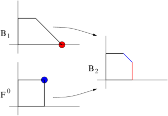
Figure 8: Equivalence of $\mathbb{B}_{2}$ and $\mathbb{F}^{1}$.

2.6 Toric description of curves and intersection numbers

As remarked earlier, each boundary line segment of the toric diagram corresponds to an exceptional curve. Let us denote the curve corresponding to $I_{i}$ by $D_{i}$; then we can see from Fig. 9 that

$$\sum_{i}D_{i}=-K\,,\,\,\,\mbox{and}\,\,\,D_{i}\cdot D_{j}=\delta_{i,j+1}+\delta_{i,j-1}\,.$$ (43)

Figure 9: a) Boundary components of the toric diagram and corresponding exceptional curves for $\mathbb{B}_{3}$, b) boundary components and corresponding exceptional curves for $\mathbb{F}^{2}$.

An equivalent way of representing curves in the del Pezzo is motivated from the string web picture in the context of $(p,q)$ 5-branes [7], which is related to del Pezzos as discussed in [5]. Namely, the del Pezzos have a symplectic form represented by the Kähler class. The base of the toric fibration can be viewed as the ‘$x$’ space and the $T^{2}$ fibers can be viewed as ‘$p$’ directions, where we represent the symplectic form as $\sum_{i=1}^{2}dx_{i}\wedge dp_{i}=\sum_{i=1}^{2}d|\Phi_{i}|^{2}\wedge d\theta_{i}$, where $\theta_{i}$ represents the phase of $\Phi_{i}$. This implies that each direction in the base is naturally paired with a circle in the fiber. Consider for example a line in the base ending on a boundary. If the line ends orthogonally on the boundary, considering the total space of the line and the corresponding circle in the fiber one obtains a piece of a holomorphic curve. We can connect these pieces together to obtain closed curves by drawing trivalent graphs with external legs ending orthogonally on the boundary components $I_{i}$. Consider first the case of $\mathbb{P}^{2}$; let us try to represent in this way the class $H$ of a line. If we can find a curve of genus zero with self-intersection one then it is clear that this curve represents $H$. As shown in Fig. 10(a), such a curve corresponds to the simplest trivalent graph in the triangle; this can be understood from the fact that the boundary components are in the same class as $H$ and therefore

$$D_{i}\cdot H=1\,,\,\,\,i=1,2,3,$$ (44)

which implies that the graph corresponding to $H$ should have one external leg ending on each $I_{i}$. In fact note that there is a moduli space for this curve (which is again a ${\mathbb{P}}^{2}$) which can be viewed in the base as the choice for the position of the trivalent vertex (this description itself gives the base of a toric realization of the moduli space). One can see that if we go to a point on the moduli space of this curve corresponding to putting the trivalent point of the graph at one of the three vertices of the triangle we obtain the curve $z_{1}=0$ which represents $H$.

Fig. 10(b) shows the case of a conic in ${\mathbb{P}}^{2}$, which has genus zero and in homology is just $2H$. It is easy to see by deforming the graph and making it trivalent that it indeed represents a curve of genus zero. On the other hand, a cubic curve will have genus one, as one sees from the “hole” appearing in the rightmost picture in Fig. 10(c).

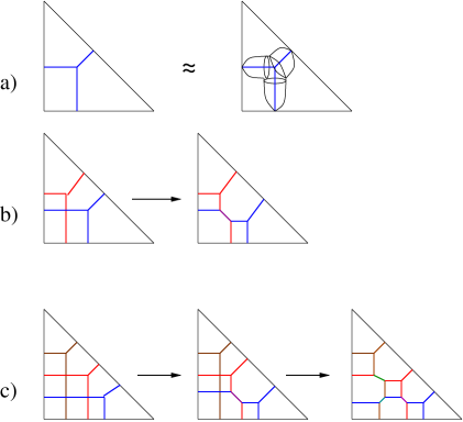
Figure 10: a) Line $H$ in $\mathbb{P}^{2}$, b) conic $2H$ in $\mathbb{P}^{2}$, c) anticanonical class $3H$ in $\mathbb{P}^{2}$.

2.7 Quadratic transformation

Now we discuss the geometric realization of the nontrivial part of the Weyl group, the reflection in $\alpha_{k}=H-E_{1}-E_{2}-E_{3}$. First consider the case $k=3$ and observe that starting from $\mathbb{B}_{3}$ we can obtain ${\mathbb{P}}^{2}$ in two distinct ways: either blow down the set $\{E_{1},E_{2},E_{3}\}$ of exceptional curves, or blow down $\{H-E_{2}-E_{3},H-E_{1}-E_{3},H-E_{1}-E_{2}\}$ to obtain ${\mathbb{P}}^{2}$, as shown in Fig. 11.

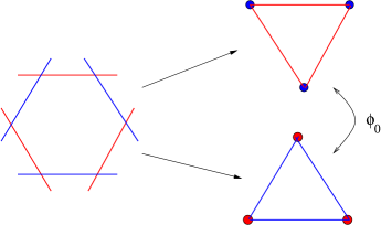
Figure 11: Blowing down from $\mathbb{B}_{3}$ to $\mathbb{P}^{2}$ in two different ways.

The two sets of exceptional curves are related to each other precisely by the reflection in the root $\alpha_{3}.$ Correspondingly, the ${\mathbb{P}}^{2}$’s obtained this way are related by a birational map $\phi_{0}$ called the “quadratic transformation,” [4] given by

$$\phi_{0}\,:\,[z_{1},z_{2},z_{3}]\,\mapsto\,[z_{2}z_{3},z_{1}z_{3},z_{1}z_{2}]\,.$$ (45)

The expression above makes sense only when at least two of the $z_{i}$ are nonzero (otherwise we get $[0,0,0]$ which is not a point of ${\mathbb{P}}^{2}$); so $\phi_{0}$ is defined on ${\mathbb{P}}^{2}$ minus the three points $x_{1}=[1,0,0],x_{2}=[0,1,0],x_{3}=[0,0,1]$. By blowing up those three points to $E_{1},E_{2},E_{3}$ we can make $\phi_{0}$ defined everywhere. Similarly, we can make $\phi_{0}$ 1-1 by blowing up the same three points in the image ${\mathbb{P}}^{2}$. We therefore obtain an automorphism of $\mathbb{B}_{3}$.

Now how does $\phi_{0}$ act on $H_{2}(\mathbb{B}_{3},{\mathbb{Z}})$? It is easy to see that

$$\phi_{0}^{2}([z_{1},z_{2},z_{3}])=[(z_{1}z_{2}z_{3})\,z_{1},(z_{1}z_{2}z_{3})\,z_{2},(z_{1}z_{2}z_{3})\,z_{3}]\,.$$ (46)

Thus $\phi_{0}^{2}$ is the identity on the open set ${\mathbb{P}}^{2}-\{z_{1}=0\}-\{z_{2}=0\}-\{z_{3}=0\}$ and hence extends to the identity on $\mathbb{B}_{3}$, so $\phi_{0}^{2}=1$ on $H_{2}(\mathbb{B}_{3},{\mathbb{Z}})$. Next let us consider the action of $\phi_{0}$ on $H-E_{1}-E_{2}$. This class is the proper transform of a complex line in ${\mathbb{P}}^{2}$ passing through the points $x_{1}$ and $x_{2}$, namely the line $z_{3}=0$. The action (45) of $\phi_{0}$ maps this line to the point $x_{3}=[0,0,1]$ which was blown up to obtain $E_{3}$; hence $\phi_{0}(H-E_{1}-E_{2})=E_{3}$. Since $\phi_{0}^{2}=1$ we also have $\phi_{0}(E_{3})=H-E_{1}-E_{2}$ and similarly for the other exceptional curves. This is precisely the action of the reflection in the root $\alpha_{3}$, as desired.

For $k>3$ the situation is similar: the presence of additional blown-up points at generic positions on ${\mathbb{P}}^{2}$ does not change anything, except that the quadratic transformation will move these points, so that we have to compose with a diffeomorphism of ${\mathbb{P}}^{2}$ to move them back to their original positions. So for all $k\geq 3$ the reflection in $\alpha_{k}$ is realized by a global diffeomorphism.

The description of the quadratic transformation above was given in terms of the realization of $\mathbb{B}_{k}$ as ${\mathbb{P}}^{2}$ blown up at $k$ points. However, as discussed above, $\mathbb{B}_{k}\simeq{\mathbb{F}}^{k+1}$ so we can equally well think of ${\mathbb{P}}^{1}\times{\mathbb{P}}^{1}$ blown up at $k-1$ points. From this perspective the action of the quadratic transformation is simple to describe: namely, it corresponds to exchanging two of the $k-1$ blown-up points. This description makes it obvious that the quadratic transformation is realized by a global diffeomorphism.

3 The correspondence

We have discussed in the previous section how the moduli spaces of del Pezzos are interrelated via the operations of blowing up and down. Moreover, as we have discussed, the group of global diffeomorphisms of $\mathbb{B}_{k}$ which fix $K$ is the Weyl group of the corresponding exceptional group $E_{k}$.

On the other hand, if we consider compactifications of M-theory on rectangular tori $T^{k}$ with no vev for the $C$-field, the U-duality group acting on this class of compactifications is also realized as the Weyl group of $E_{k}$ [8] (see also [9].) It is thus natural to ask if there is a map between such M-theory compactifications and del Pezzo geometries. In fact, the story is already rather interesting for small $k$’s, as shown in Fig. 12.

Figure 12: M-theory / del Pezzo relation for $k=0,1,2,3$.

Note that in Fig. 12 each time we blow up a point to a ${\mathbb{P}}^{1}$ in the del Pezzo, we compactify a circle on the M-theory side. It is remarkable that the exotic role type IIB plays in the chain of dualities of M-theory exactly matches the role ${\mathbb{P}}^{1}\times{\mathbb{P}}^{1}$ plays among del Pezzos. In particular, if we wish to get from M-theory in 11-dimensions to type IIB in 10 dimensions, we have to compactify two circles and then let the resulting torus shrink to zero size; this is precisely mirrored by the fact that to get to ${\mathbb{P}}^{1}\times{\mathbb{P}}^{1}$ from ${\mathbb{P}}^{2}$ we first have to blow up two points and then blow down another ${\mathbb{P}}^{1}$. Note also that the symmetries of the corresponding theories are manifest as classical symmetries of the del Pezzos. For example, the $S$-duality of type IIB corresponds to the exchange of the two sides of the rectangle above (i.e. the exchange of the two ${\mathbb{P}}^{1}$’s). Moreover, the non-trivial part of S-duality in M-theory compactified to 9 dimensions is still ${\mathbb{Z}}_{2}$, which is reflected in the ${\mathbb{Z}}_{2}$ symmetry of the rectangle with one corner cut off. The non-trivial part of S-duality in $d=8$ is ${\mathbb{Z}}_{2}\times S_{3}$, which is manifest as the symmetries of the del Pezzo $\mathbb{B}_{3}$, torically represented by the group of symmetries of the hexagon depicted in the above figure. Indeed this identification of Weyl groups continues to make sense for all del Pezzos, even those which are not toric (namely the $\mathbb{B}_{k}$ with $k>3$).

It is thus natural to expect that we can get a more detailed map between the two sides and promote the above correspondence to the level of moduli and objects on both sides. We now consider this question.

3.1 Matching the moduli spaces

We consider the moduli space for M-theory on a geometry $T^{k}\times{\mathbb{R}}^{10-k,1}$ for $k\leq 8$, where the torus has a rectangular metric of the form

$$ds^{2}=\sum_{i=1}^{k}R_{i}^{2}dx_{i}^{2}$$ (47)

with the $x_{i}$ periodic, $x_{i}\sim x_{i}+2\pi$, and all background $C$ fields set to zero.

At least when all $R_{i}$ are small compared to the $11$ dimensional Planck scale $l_{p}$, the low energy dynamics are described by an $11-k$ dimensional supergravity theory with $32$ supercharges. This theory is determined by the $k+1$ parameters $l_{p},R_{1},\dots,R_{k}$ which are positive real numbers, so naively one would expect its moduli space to be ${\mathbb{R}}_{+}^{k+1}$. However, if we want the space of physically inequivalent theories then we have to take the quotient of ${\mathbb{R}}_{+}^{k+1}$ by the duality group consisting of transformations which leave the physics invariant.

For M-theory on a $T^{k}$ of arbitrary shape with arbitrary $C$-field the duality group is well known to be $E_{k(k)}({\mathbb{Z}})$ [10]. In our case we want to consider only dualities which respect the “rectangular, no $C$-field” condition. These include the symmetric group $S_{k}$ permuting the $k$ radii; this group is generated by the $k-1$ exchanges

$$w_{\alpha_{i}}:R_{i}\leftrightarrow R_{i+1},\,\,i=1,\dots,k-1.$$ (48)

In addition one also has the action of T-duality (M2/M5 exchange, after $T^{3}$ compactification) which when expressed in M-theory language involves three radii, so we need to include one extra generator in case $k\geq 3$, namely

$$w_{\alpha_{k}}:2\pi R_{1}\mapsto\frac{l_{p}^{3}}{2\pi R_{2}2\pi R_{3}},2\pi R_{2}\mapsto\frac{l_{p}^{3}}{2\pi R_{1}2\pi R_{3}},2\pi R_{3}\mapsto\frac{l_{p}^{3}}{2\pi R_{1}2\pi R_{2}},l_{p}^{3}\mapsto\frac{l_{p}^{6}}{2\pi R_{1}2\pi R_{2}2\pi R_{3}}.$$ (49)

As we will see below, this corresponds to the quadratic transformation discussed before in the context of del Pezzos. It is known [9, 11] that the $w_{\alpha_{i}}$ generate the full duality group acting on “rectangular, no $C$-field” compactifications; just as in Section 2.3 this group is isomorphic to the Weyl group of $E_{k}$. Moreover, the other elements of the U-duality group, such as periodicity of the $C$ field or shifting complex moduli of tori by $\tau\rightarrow\tau+1$, are manifest symmetries of string theory. So the non-obvious part of the full U-duality group is already captured by the Weyl group $W(E_{k})$.

Now we are ready to map the moduli. Using the notation $\widehat{\mathcal{M}_{k}}$ for the naive moduli space ${\mathbb{R}}^{k+1}_{+}$, we may write

$$\mathcal{M}_{k}=\widehat{\mathcal{M}_{k}}/W(E_{k}).$$ (50)

It is convenient to switch to a linear representation by taking logarithms: namely, we think of $\widehat{\mathcal{M}_{k}}$ as a $(k+1)$-dimensional real vector space, with a typical element

$$(\log l_{p},\log(2\pi R_{1}),\dots,\log(2\pi R_{k})).$$ (51)

Then $U_{k}$ acts linearly on $\widehat{\mathcal{M}_{k}}$. To establish our correspondence we need one more piece of structure on $\widehat{\mathcal{M}_{k}}$. Namely, by considering the log-tension formulas for $\frac{1}{2}$-BPS states we obtain a lattice $\Lambda$ in the dual vector space $\widehat{\mathcal{M}_{k}}^{*}$, spanned by $k+1$ basis vectors $(3\log l_{p})$ and $(\log 2\pi R_{a})$ ($a=1,\dots,k$).

In sum, we have a $(k+1)$-dimensional vector space $\widehat{\mathcal{M}_{k}}$, carrying an action of the Weyl group $U_{k}$ which furthermore preserves a lattice $\Lambda$ in the dual space. Precisely this structure is also present on the del Pezzo surface: namely, we have the $(k+1)$-dimensional cohomology $H^{2}(\mathbb{B}_{k},{\mathbb{R}})$, carrying an action of the Weyl group by global diffeomorphisms preserving the canonical class, which furthermore preserves the homology lattice $H_{2}(\mathbb{B}_{k},{\mathbb{Z}})$. The natural thing to do, then, is to identify the two vector spaces $H_{2}(\mathbb{B}_{k},{\mathbb{R}})$ and $\widehat{\mathcal{M}_{k}}^{*}$ in a way which identifies the lattices $H_{2}(\mathbb{B}_{k},{\mathbb{Z}})$ and $\Lambda$ while preserving the action of the Weyl group. This can be done in an essentially unique way: in the notation of Section 2.1, we map

$$H\mapsto -3\log l_{p},$$ (52)

$$E_{a}\mapsto -\log(2\pi R_{a}).$$

Dually, we have an identification between $\widehat{\mathcal{M}_{k}}$ and $H^{2}(\mathbb{B}_{k},{\mathbb{R}})$, described by

$$(l_{p},R_{1},\dots,R_{k})\leftrightarrow(\omega\in H^{2}(\mathbb{B}_{k},{\mathbb{R}}):\ \omega(H)=-3\log l_{p},\omega(E_{a})=-\log(2\pi R_{a})).$$ (53)

We think of $\omega\in H^{2}(\mathbb{B}_{k},{\mathbb{R}})$ as a kind of generalized Kähler class. If $\omega$ came from an ordinary (positive) Kähler metric, then $\omega({\mathcal{C}})$ would be simply the volume of a holomorphic curve in the class ${\mathcal{C}}$. Our $\omega$ need not come from a Kähler metric, since $\omega({\mathcal{C}})$ may be negative (e.g. if $2\pi R_{a}>1$ then $\omega(E_{a})<0$.)

The choice (52) is not quite unique — apart from the unimportant freedom to make a Weyl group transformation on one side, we could also have taken plus signs instead of minus. Our choice was dictated by the original intuition that blowing up $E_{a}$ corresponds to compactification from $R_{a}=\infty$ to $R_{a}=\mathrm{finite}$, so that the volume of $E_{a}$ should be inversely related to $R_{a}$.

Before going further, let us remark on the appearance of the group of diffeomorphisms preserving the canonical class $K$ in the above correspondence. Recall from (6) that

$$K=-3H+\sum_{a=1}^{k}E_{a}.$$ (54)

Applying (52) we find the correspondence

$$K\mapsto(9-k)\log\widetilde{l_{p}},$$ (55)

where $\widetilde{l_{p}}$ is the Planck length in the compactified theory, which is given by

$$\widetilde{l_{p}}^{9-k}=\frac{l_{p}^{9}}{(2\pi R_{1})\cdots(2\pi R_{k})}.$$ (56)

Since $\widetilde{l_{p}}^{9-k}$ can be observed in the dimensionally reduced theory as the inverse of the gravitational coupling constant, it must be invariant under every element in the U-duality group; this is why we have to consider only diffeomorphisms preserving $K$.

3.2 Brane charges and rational curves

Next we consider the tensions of $\frac{1}{2}$-BPS states in M-theory. We will show that a holomorphic rational curve ${\mathcal{C}}$ in the del Pezzo corresponds to a $\frac{1}{2}$-BPS $p$-brane charge. Moreover, the BPS tension can be identified as

$$T=2\pi\exp\omega({\mathcal{C}}),$$ (57)

where $\omega\in H^{2}(\mathbb{B}_{k},{\mathbb{R}})$ is the generalized Kähler class introduced in the last section. Given this formula for the tension, one easily checks that $p$ is determined by the intersection product with $K$ (recall that $K$ corresponds to $(9-k)\log\widetilde{l_{p}}$, so we can think of it as in some sense “carrying the units of mass”):

$$d_{{\cal C}}=-{\mathcal{C}}\cdot K=p+1.$$ (58)

Furthermore, electric-magnetic duality has a simple interpretation in this framework: dual pairs are related simply by

$${\mathcal{C}}_{\mathrm{Electric}}+{\mathcal{C}}_{\mathrm{Magnetic}}=-K.$$ (59)

In particular this will imply, using (57) and (55), that

$$T_{\mathrm{Electric}}T_{\mathrm{Magnetic}}=(2\pi)^{2}\widetilde{l_{p}}^{k-9},$$ (60)

for all electric-magnetic pairs of $\frac{1}{2}$-BPS branes.

Before considering the general setup, let us consider the simple case of uncompactified M-theory.

M-theory in $d=11$. Recall that this theory corresponds to ${\mathbb{P}}^{2}$. The lattice $H_{2}({\mathbb{P}}^{2},{\mathbb{Z}})$ is spanned by the single element $H$, so consider a curve in ${\mathbb{P}}^{2}$ given by the class

$${\mathcal{C}}=n\,H.$$ (61)

A priori we could choose any integral value for $n$. However, not every class in $H_{2}({\mathbb{P}}^{2},{\mathbb{Z}})$ is actually realized by a holomorphic curve: one has to choose $n>0$. Choosing $n=1$, $H$ is the class of a line in ${\mathbb{P}}^{2}$, and the tension formula gives $T=2\pi\exp\omega(H)=2\pi/l_{p}^{3}$. Similarly, $2H$ is the class of a conic and gives $T=2\pi/l_{p}^{6}$, the tension of the M5 brane. These are the only genus zero curves in $\mathbb{P}^{2}$, since by (10) the genus of ${\mathcal{C}}=nH$ is given by

$$g({\mathcal{C}})=\frac{(n-1)(n-2)}{2}\,.$$ (62)

The toric representations of $H$ and $2H$ are shown in Fig. 13.

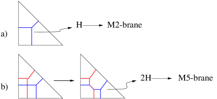
Figure 13: a) Hyperplane class $H$ in $\mathbb{P}^{2}$ which maps to the M2-brane, b) The conic $2H$ in $\mathbb{P}^{2}$ which maps to the M5-brane.

Note that the fact that the M2-brane and M5-brane are electric-magnetic duals agrees with the prediction from (59), because $H+2H=3H=-K_{{\mathbb{P}}^{2}}$.

What about $3H$? This is the class of a cubic curve in ${\mathbb{P}}^{2}$. If it plays a role in our correspondence it should correspond to a tension $T=2\pi/l_{p}^{9}$, giving some hypothetical M8 brane. On the other hand, as remarked earlier, a cubic curve in ${\mathbb{P}}^{2}$ has genus one. So if we restrict to rational curves we obtain only the M2 and M5.

It is intriguing that the fact that the worldvolume dimensions of the $\frac{1}{2}$-BPS states in $11$ dimensions are a multiple of $3$ directly follows from the fact that the canonical class of ${\mathbb{P}}^{2}$ is a multiple of $3$ given by $-3H$. This is indeed a remarkable map!

Before going on to a more complicated example, we discuss some general aspects of the relevant physics. States which are $\frac{1}{2}$-BPS satisfy a formula relating their tensions to the SUSY central charges. These charges in turn are proportional to gauge charges in $11-k$ dimensions, with the constant of proportionality depending on the parameters $R_{a}$ and $l_{p}$. For example, a state with one unit of momentum in the compact $1$ direction would satisfy

$$M=\frac{1}{R_{1}},$$ (63)

while an M2-brane wrapped on the $1-2$ directions would have

$$M=\frac{(2\pi)^{3}R_{1}\,R_{2}}{l_{p}^{3}}.$$ (64)

By “gauge charge” we include charges under $p$-form symmetries as well as $1$-forms, so we can also consider e.g. an M5 wrapped on the $1-2-3$ directions. In this case we get a tension formula rather than a mass formula, which reads

$$T=\frac{(2\pi)^{4}\,R_{1}\,R_{2}\,R_{3}}{l_{p}^{6}}.$$ (65)

All three tension formulas (63), (64), (65) are of the form

$$T=2\pi\frac{(2\pi R_{1})^{m_{1}}\cdots(2\pi R_{k})^{m_{k}}}{l_{p}^{3n}},$$ (66)

with $n$ and all $m_{a}$ integral. It is not quite true that this is the most general situation for a $\frac{1}{2}$-BPS state — for example, a state with one unit of momentum in each of the $1$ and $2$ directions would have $M=\sqrt{1/R_{1}^{2}+1/R_{2}^{2}}$. Put differently, the two states given by one unit of momentum in each of the $1$ and $2$ directions form a bound state which has mass smaller than the sum of the two masses. We will discuss below the geometric condition under which a pair of $\frac{1}{2}$-BPS states form a bound state; at this point we concentrate on a particular basis for the lattice of charges, such that every state in the basis has a tension formula of the form (66).

So let us relate the formula (66) to the del Pezzo surface $\mathbb{B}_{k}$. Setting

$$V=-3n\log l_{p}+\sum_{a=1}^{k}m_{a}\log(2\pi R_{a}),$$ (67)

we can rewrite (66) as

$$T=2\pi\exp V.$$ (68)

On the other hand, through the map (53) we can rewrite (67) as

$$V=\omega({\mathcal{C}}),$$ (69)

where

$${\mathcal{C}}=nH-\sum_{a=1}^{k}m_{a}E_{a}.$$ (70)

So we have expressed the log-tensions of certain $\frac{1}{2}$-BPS states as generalized volumes of particular classes in $H_{2}(\mathbb{B}_{k},{\mathbb{Z}})$, using (52) as our dictionary.

We can now ask the question: which classes actually do correspond to $\frac{1}{2}$-BPS states? We will see below that the rational curves which correspond to $p$-branes with codimension 2 or more are in 1-1 correspondence with the $\frac{1}{2}$-BPS brane charges in M-theory. We have already discussed the situation for M-theory in 11 dimensions. Let us now consider its compactification to 10 dimensions.

Type IIA in $d=10$. Compactifying M-theory on a circle corresponds to blowing up a point on ${\mathbb{P}}^{2}$ to get $\mathbb{B}_{1}$. The homology lattice is then two-dimensional, so an arbitrary element in $H_{2}(\mathbb{B}_{1},{\mathbb{Z}})$ is given by

$${\mathcal{C}}=nH-mE.$$ (71)

Taking our cue from the result in case $k=0$, let us look for ${\mathcal{C}}$ which are realized by holomorphic curves of genus zero. The adjunction formula (10) in this case becomes

$$n(n-3)+m(m-1)=2g-2.$$ (72)

Looking for integer solutions of the resulting quadratic, we find two infinite families:

$$(n,m)=\left(\frac{p}{2},\frac{p}{2}-1\right) \ \ (p\in 2{\mathbb{Z}})$$ (73)

$$(n,m)=\left(\frac{p+3}{4},-\frac{p-5}{4}\right) \ \ (p\in 4{\mathbb{Z}}+1).$$

Since we do not have branes of arbitrary dimension in type IIA, we now impose a further restriction: namely, we consider only solutions with $0\leq p\leq 8$. Upon so doing we obtain the following list:

homology class	tension	type IIA meaning
$E$	$R^{-1}=l_{s}^{-1}g_{s}^{-1}$	D0-brane
$H-E$	$(2\pi)^{2}\,Rl_{p}^{-3}=(2\pi)^{-1}l_{s}^{-2}$	F-string
$H$	$(2\pi)\,l_{p}^{-3}=(2\pi)^{-2}\,l_{s}^{-3}g_{s}^{-1}$	D2-brane
$2H-E$	$(2\pi)^{2}\,Rl_{p}^{-6}=(2\pi)^{-4}\,l_{s}^{-5}g_{s}^{-1}$	D4-brane
$2H$	$(2\pi)\,l_{p}^{-6}=(2\pi)^{-5}\,l_{s}^{-6}g_{s}^{-2}$	NS5-brane
$3H-2E$	$(2\pi)^{3}\,R^{2}l_{p}^{-9}=(2\pi)^{-6}\,l_{s}^{-7}g_{s}^{-1}$	D6-brane
$4H-3E$	$(2\pi)^{4}\,R^{3}l_{p}^{-12}=(2\pi)^{-8}\,l_{s}^{-9}g_{s}^{-1}$	D8-brane

Remarkably, we have all the relevant $\frac{1}{2}$-BPS objects in type IIA in 10 dimensions, with the correct tensions. To see this, consider the $p$-brane which maps to the curve ${\mathcal{C}}_{n,m}=nH-mE$, for some $n$ and $m$ satisfying (73). The tension is given by

$$T_{n,m} =2\pi\,\mbox{exp}(\omega({\mathcal{C}}_{n,m}))\,,$$ (74)

$$=2\pi\,\frac{(2\pi R)^{m}}{l_{p}^{3n}}\,.$$

From (74) it follows that

$$T_{Dp-brane} =T_{\frac{p}{2},\frac{p}{2}-1}=\frac{(2\pi)^{\frac{p}{2}}\,R^{\frac{p}{2}-1}}{l_{p}^{\frac{3p}{2}}}\,=\,\frac{1}{(2\pi)^{p}\,g_{s}\,l_{s}^{p+1}}\,,$$ (75)

$$T_{NSp-brane} =T_{\frac{p+3}{4},\frac{5-p}{4}}=\frac{(2\pi)^{\frac{9-p}{4}}\,R^{\frac{5-p}{4}}}{l_{p}^{\frac{2p+9}{4}}}\,=\,\frac{1}{(2\pi)^{p}\,g_{s}^{\frac{p-1}{2}}\,l_{s}^{p+1}}\,.$$

Thus we get correct tensions for all the D$p$-brane as well as the fundamental string and the NS5-brane, as shown in the above table.

The electric/magnetic pairing works as described by (59), with

$${\mathcal{C}}_{\mathrm{Electric}}+{\mathcal{C}}_{\mathrm{Magnetic}}=-K=3H-E.$$ (76)

It is also interesting that the del Pezzo knows about ALF space, i.e. about the D6 brane, which does not come from simple dimensional reduction from 11 dimensions. Similarly the appearance of the D8 brane here, which does not correspond to any object in ${\mathbb{P}}^{2}$, is remarkable.

Type II in $d=8$. For brevity we now skip $d=9$ and go directly to $d=8$. We search for curves which could represent $p$-branes with $0\leq p\leq 6$; using (10) as above and (58), this amounts to finding integer solutions of

$$3n-m_{1}-m_{2}-m_{3} =p+1,$$ (77)

$$n^{2}-m_{1}^{2}-m_{2}^{2}-m_{3}^{2} =p-1.$$

The results are summarized in the table below, where we include the interpretation of the states in terms of M-theory as well as Type IIA. (One could also interpret these states from the perspective of compactified Type IIB, using the relations (5) between blow-ups of ${\mathbb{P}}^{2}$ and of ${\mathbb{P}}^{1}\times{\mathbb{P}}^{1}$.)

$p$	homology class	type IIA meaning	M-theory meaning
$p=0$	$E_{M}$	D0-brane	momentum
	$E_{i}$	momentum
	$H-E_{i}-E_{j}$	twice-wrapped D2-brane	twice-wrapped M2-brane
	$H-E_{M}-E_{i}$	once-wrapped F-string
$p=1$	$H-E_{M}$	F-string	once-wrapped M2-brane
	$H-E_{i}$	once-wrapped D2-brane
$p=2$	$H$	D2-brane	M2-brane
	$2H-E_{M}-E_{i}-E_{j}$	twice-wrapped D4-brane	thrice-wrapped M5-brane
$p=3$	$2H-E_{M}-E_{i}$	once-wrapped D4-brane	twice-wrapped M5-brane
	$2H-E_{i}-E_{j}$	twice-wrapped NS5-brane
$p=4$	$2H-E_{M}$	D4-brane	once-wrapped M5-brane
	$2H-E_{i}$	once-wrapped NS5-brane
	$3H-2E_{M}-E_{i}-E_{j}$	twice-wrapped D6-brane	twice-wrapped ALF space
	$3H-E_{M}-2E_{i}-E_{j}$	exotic state
$p=5$	$2H$	NS5-brane	M5-brane
	$3H-2E_{M}-E_{i}$	once-wrapped D6-brane	once-wrapped ALF space
	$3H-E_{M}-2E_{i}$	exotic state
	$3H-2E_{i}-E_{j}$	exotic state
	$4H-2E_{M}-2E_{i}-2E_{j}$	exotic state	exotic state
$p=6$	$3H-2E_{M}$	D6-brane	ALF space
	$3H-2E_{i}$	exotic state
	$4H-3E_{M}-E_{i}-E_{j}$	twice-wrapped D8-brane	exotic state
	$4H-E_{M}-3E_{i}-E_{j}$	exotic state

In the above table we have singled out one of the exceptional curves as the “M-theory direction” and called it $E_{M}$, while the indices $i,j$ run over the values $1,2$ for the other two circles. The entries labeled “exotic state” correspond to states satisfying exotic tension formulas which are not straightforward to interpret; nevertheless, these states are required by the U-duality symmetry, as reviewed e.g. in [11].

From looking at the table we notice a simple pattern, namely, if ${\mathcal{C}}$ is a $\frac{1}{2}$-BPS object not involving $E_{i}$, then ${\mathcal{C}}-E_{i}$ will be the same object wrapped on the $i$ direction. One can also see this directly from the tension formulas since $-E_{i}$ corresponds to $\log 2\pi R_{i}$.

Type IIB in $d=10$. In our discussion so far we have mostly stuck to the surfaces $\mathbb{B}_{k}$, but the discussion goes through essentially unchanged for ${\mathbb{P}}^{1}\times{\mathbb{P}}^{1}$. Recall that a basis for $H_{2}({\mathbb{P}}^{1}\times{\mathbb{P}}^{1},{\mathbb{Z}})$ is given by the classes of the two factors, which we write $l_{1}$ and $l_{2}$, with

$$l_{1}\cdot l_{1}=l_{2}\cdot l_{2} =0,$$ (78)

$$l_{1}\cdot l_{2} =1.$$

The canonical class is $K=-2l_{1}-2l_{2}$, and the analog of (52) in this setting is

$$l_{1} \mapsto-2\log 2\pi l_{s},$$ (79)

$$l_{1} \mapsto-2\log 2\pi l_{s}-\log g_{s},$$

where $l_{s}$ and $g_{s}$ now denote the Type IIB quantities. From (9) and (10), a genus zero curve ${\cal C}=nl_{1}+ml_{2}$ of degree $p+1$ satisfies

$$2nm=p-1\,,\,\,\,2(n+m)=p+1\,.$$ (80)

There are two integer solutions for each $p\in 2{\mathbb{Z}}+1$:

$$(n,m) =\left(1,\frac{p-1}{2}\right)\,,$$ (81)

$$(n,m) =\left(\frac{p-1}{2},1\right)\,.$$

The tension is then given by

$$T_{Dp-brane} =T_{\frac{p-1}{2},1}=\frac{1}{(2\pi)^{\frac{p-1}{2}}}\,T_{F-string}^{\frac{p-1}{2}}\,T_{D-string}=\frac{1}{(2\pi)^{p}\,g_{s}\,l_{p}^{p+1}}\,,$$ (82)

$$T_{NSp-brane} =T_{1,\frac{p-1}{2}}=\frac{1}{(2\pi)^{\frac{p-1}{2}}}\,T_{F-string}\,T_{D-string}^{\frac{p-1}{2}}=\frac{1}{(2\pi)^{p}\,g_{s}^{\frac{p-1}{2}}\,l_{p}^{p+1}}\,.$$

Then restricting to $0\leq p\leq 8$, we obtain

homology class	tension / $2\pi$	type IIB meaning
$l_{1}$	$(2\pi l_{s})^{-2}$	F-string
$l_{2}$	$(2\pi l_{s})^{-2}g_{s}^{-1}$	D-string
$l_{1}+l_{2}$	$(2\pi l_{s})^{-4}g_{s}^{-1}$	D3-brane
$2l_{1}+l_{2}$	$(2\pi l_{s})^{-6}g_{s}^{-1}$	D5-brane
$l_{1}+2l_{2}$	$(2\pi l_{s})^{-6}g_{s}^{-2}$	NS5-brane
$3l_{1}+l_{2}$	$(2\pi l_{s})^{-8}g_{s}^{-1}$	D7-brane
$l_{1}+3l_{2}$	$(2\pi l_{s})^{-8}g_{s}^{-3}$	NS7-brane

Note that the fact that the worldvolume dimension of the Type IIB $\frac{1}{2}$-BPS branes are all even follows from the fact that $K$ for ${\mathbb{P}}^{1}\times{\mathbb{P}}^{1}$ is even, i.e. $K=-2l_{1}-2l_{2}$.

Type II in general $d\geq 3$. In parallel to the discussion above, one can check that all the $\frac{1}{2}$-BPS $p$-branes with codimension at least 1 in uncompactified spacetime in compactifications of M-theory on $T^{k}$ for $k\leq 8$ are in 1-1 correspondence with rational curves ${\mathcal{C}}$ with $d_{{\cal C}}=p+1$. One finds all the branes which appeared in the table for $d=8$, plus their compactifications, plus various extra exotic states (again, all required to exist by U-duality.) It is not actually difficult to determine genus zero curves of a given degree satisfying the adjunction formula. We can write the self-intersection of ${\mathcal{C}}$ in terms of the weight vector ${\mathcal{C}}_{\perp}$ as discussed in section 2.2,

$${\mathcal{C}}^{2}=d_{{\mathcal{C}}}-2\,\,\implies{\mathcal{C}}_{\perp}^{2}=-\frac{d_{{\mathcal{C}}}^{2}}{9-k}+d_{{\mathcal{C}}}-2\,.$$ (83)

The results are summarized in the following table in which we give the representation of $E_{k}$ to which the curve belongs, the size of the Weyl orbit and a representative curve. The uncompactified dimension of spacetime is $d=11-k$.

$k$	$E_{k}$	$d_{{\mathcal{C}}}$	${\mathcal{C}}_{\perp}^{2}$	rep of $E_{k}$	Weyl orbit size	curve
$k=4$	$SU(5)$	1	$-\frac{6}{5}$	${\bf 10}$	10	$E_{1}$
		2	$-\frac{4}{5}$	${\bf 5}$	5	$H-E_{1}$
		3	$-\frac{4}{5}$	${\bf 5}$	5	$H$
		4	$-\frac{6}{5}$	${\bf 10}$	10	$3H-2E_{1}-E_{2}-E_{3}-E_{4}$
		5	$-2$	${\bf 24}$	20	$2H-E_{1}$
		6	$-\frac{16}{5}$	${\bf 15}$	5	$2H$
$k=5$	$SO(10)$	1	$-\frac{5}{4}$	${\bf 16}$	16	$E_{1}$
		2	$-1$	${\bf 10}$	10	$H-E_{1}$
		3	$-\frac{5}{4}$	${\bf 16}$	16	$3H-2E_{1}-\sum_{i=2}^{5}E_{i}$
		4	$-2$	${\bf 45}$	40	$2H-E_{1}-E_{2}$
		5	$-\frac{13}{4}$	${\bf 144}$	80	$2H-E_{1}$
$k=6$	$E_{6}$	1	$-\frac{4}{3}$	${\bf 27}$	27	$E_{1}$
		2	$-\frac{4}{3}$	${\bf 27}$	27	$3H-2E_{1}-\sum_{i=2}^{6}E_{i}$
		3	$-2$	${\bf 78}$	72	$H$
		4	$-\frac{10}{3}$	${\bf 351}$	216	$2H-E_{1}-E_{2}$
$k=7$	$E_{7}$	1	$-\frac{3}{2}$	${\bf 56}$	56	$E_{1}$
		2	$-2$	${\bf 133}$	126	$H-E_{1}$
		3	$-\frac{7}{2}$	${\bf 912}$	576	$H$
$k=8$	$E_{8}$	1	$-2$	${\bf 248}$	240	$E_{1}$
		2	$-4$	${\bf 3875}$	2160	$H-E_{1}$

3.3 Bound states of 0-branes

Consider two 0-branes, represented by rational curves ${\mathcal{C}}_{1},{\mathcal{C}}_{2}$. Then we may ask: can they form a BPS bound state? For simplicity let us restrict our attention to compactifications to $d\geq 5$ dimensions. Then there are three different possibilities: i) they form a bound state at threshold which is still $\frac{1}{2}$-BPS, ii) they form a bound state, not at threshold, which is $\frac{1}{2}$-BPS, iii) they form a bound state at threshold which is $\frac{1}{4}$-BPS. The first possibility is exemplified by a bound state of a pair of D0-branes. The second is exemplified by a bound state of a D0-brane with a 2-cycle wrapped D2-brane, and the last occurs e.g. for the bound state of a D0-brane with a 4-cycle wrapped D4-brane. It is not too difficult to show that on $\mathbb{B}_{6}$, ${\mathcal{C}}_{1}\cdot{\mathcal{C}}_{2}$ is the only Weyl invariant of a pair of exceptional curves and can only be $-1,0$ or $1$. These correspond to the above three possibilities:

$${\rm\frac{1}{2}-BPS\ at\ threshold}\leftrightarrow{\mathcal{C}}_{1}\cdot{\mathcal{C}}_{2}=-1\ \ (\mathrm{i.e.}\ {\mathcal{C}}_{1}={\mathcal{C}}_{2})$$

$${\rm\frac{1}{2}-BPS\ not\ at\ threshold}\leftrightarrow{\mathcal{C}}_{1}\cdot{\mathcal{C}}_{2}=0$$

$${\rm\frac{1}{4}-BPS\ at\ threshold}\leftrightarrow{\mathcal{C}}_{1}\cdot{\mathcal{C}}_{2}=1.$$

The mass of the bound state can be written in all three cases as

$$M_{12}=2\pi|e^{V_{1}}+i^{({\mathcal{C}}_{1}\cdot{\mathcal{C}}_{2})^{2}-1}e^{V_{2}}|.$$

Representatives of these three different cases can be chosen from the list of possible 0-brane classes (20):

$${\mathcal{C}}_{1}\cdot{\mathcal{C}}_{2} = -1\,,\qquad{\mathcal{C}}_{1}=E_{a}\,,\quad{\mathcal{C}}_{2}=E_{a}\,,$$ (84)

$${\mathcal{C}}_{1}\cdot{\mathcal{C}}_{2} = \,\,\,\,0\,,\qquad{\mathcal{C}}_{1}=E_{a}\,,\quad{\mathcal{C}}_{2}=E_{b}\,,$$

$${\mathcal{C}}_{1}\cdot{\mathcal{C}}_{2} = \,\,\,\,1\,,\qquad{\mathcal{C}}_{1}=E_{M}\,,\quad{\mathcal{C}}_{2}=2H-E_{M}-E_{1}-E_{2}-E_{3}-E_{4}\,.$$

3.4 Changes of scale

In our discussion to this point we have implicitly assumed that some energy scale $\mu$ has been fixed, with all quantities measured in units of $\mu$. Indeed, such a choice is necessary in order to make sense of our main formula (57), $T=2\pi\exp\omega({\mathcal{C}})$, which requires that $T$ be dimensionless. To understand the significance of this choice let us write the $\mu$ dependence explicitly: then for a $p$-brane state corresponding to a curve ${\mathcal{C}}$,

$$\log(T/2\pi\mu^{p+1})=\omega({\mathcal{C}}).$$ (85)

Now consider changing scale from $\mu$ to $\mu^{\prime}$; then we will have

$$\log(T/{2\pi\mu^{\prime}}^{p+1})=\log(T/{2\pi\mu}^{p+1})+(p+1)\log(\mu/\mu^{\prime})=\omega({\mathcal{C}})+(p+1)\log(\mu/\mu^{\prime}).$$ (86)

On the other hand, using (58) we can also rewrite (86) as

$$\log(T/{2\pi\mu^{\prime}}^{p+1})=\omega^{\prime}({\mathcal{C}}),$$ (87)

where

$$\omega^{\prime}({\mathcal{C}})=\omega({\mathcal{C}})+\log(\mu/\mu^{\prime}){\mathcal{C}}\cdot K.$$ (88)

Hence a change in $\mu$ is equivalent to a shift in the generalized Kähler class $\omega$ along the direction of $K$. In particular, shifts along the $K$ direction do not affect any dimensionless quantities one might compute on the M-theory side (e.g. ratios of masses of $\frac{1}{2}$-BPS states.) So it is natural to think of $\omega$ as decomposed into

$$\omega=\omega_{\perp}+\lambda K$$ (89)

where $\omega_{\perp}$ is orthogonal to $K$; then $\omega_{\perp}$ controls all the dimensionless quantities and $\lambda$ sets the units of measurement. Setting $\mu=\widetilde{l_{p}}$ would correspond to fixing $\lambda=0$ in (89).

The situation just described is somewhat counterintuitive: one might have expected that the choice of units in M-theory would correspond to the overall volume of the del Pezzo, but the exponential relation between volumes and masses spoils that idea. In particular, given any $\omega\in H^{2}(X,{\mathbb{R}})$, there is some $\lambda$ for which $\omega+\lambda K$ is in the Kähler cone; so if we interpret $\omega$ as a generalized metric, then whether volumes of curves on the del Pezzo are positive or not is dependent on the units we choose.

4 Concluding discussion

The duality we have described is mathematically rather striking. Of course, it is important to uncover its physical interpretation. It is hard to believe that the correspondence is purely accidental (it is reminiscent of the purely “accidental” appearance of Dynkin diagrams in the intersection matrix of vanishing 2-cycles in $K3$). One possibility is that the del Pezzo is the moduli space of some probe in M-theory. If so this probe must be a U-duality invariant probe, and should be unlike any brane with which we are familiar. However, we can obtain a hint about what it should be from the del Pezzo side. Recall that the U-duality group was mapped to the group of global diffeomorphisms of del Pezzo which preserve $K$. Thus a curve in the class given by $-K$ will be U-duality invariant. Such a curve would have genus one (it is the elliptic curve in ${\mathbb{P}}^{2}$, with the blow-up classes added.) Up to now we have only considered rational curves, but if we assume there is a $p$-brane associated to this duality invariant elliptic curve, then we get

$$p+1=(-K)\cdot(-K)=9-k$$

i.e., it would be an $8-k$-brane, which would have codimension 2 in the uncompactified spacetime. It would be interesting to see if such a U-duality invariant brane exists in some sense, and if so whether its moduli space is given by the del Pezzo.

A rather interesting suggestion has been made by Motl: perhaps the del Pezzos should be viewed as target spaces of $(2,1)$ strings, thus providing a concrete realization of the proposal [13]. There are a number of obstacles to overcome to make this precise, but there are encouraging signs that this idea may be on the right track [15].

Up to now, we have considered only rectangular compactifications of M-theory, with the $C$ fields vanishing. It is natural to ask how we can relax these conditions. If we fix $\widetilde{l_{p}}$ then by a naive dimension count we find that the tangent space to the moduli space of M-theory compactifications could correspond to

$$\bigoplus_{p=1,2,3,6}\Lambda^{p}(H^{2}_{\perp}(\mathbb{B}_{k})),$$

where the symbol $\perp$ means we restrict to the subspace orthogonal to $K$. The rectangular compactifications correspond to $p=1$ above; this is the map we have already described. The $p=2$ can be viewed as the choice of making parallelogram compactification of tori, $p=3$ is turning on the $C$-field and $p=6$ corresponds to turning on the 6-form field coupling to the M5-brane (for compactifications to 3-dimensions some other exotic moduli appear). It would be interesting to interpret the $p\neq 1$ deformations in some geometric way. Similarly, it would be useful to have a clearer geometric understanding of the role of $\frac{1}{2}$-BPS states whose masses are not of the simple form (66).

It would also be interesting to extend this kind of duality to other compactifications of M-theory. A natural candidate to study in this case is the duality web with 16 supercharges.

Appendix: Group-theoretic description

To emphasize the mathematical naturality of our construction, we recall a more abstract description of the moduli space of M-theory on $T^{k}$ with $\widetilde{l_{p}}$ held fixed: namely, the moduli space is of the form $G({\mathbb{Z}})\backslash G/K$, where $G=E_{k(k)}({\mathbb{R}})$ is the maximally noncompact real form of $E_{k}$, and $K$ is a maximal compact subgroup. Restricting to rectangular tori with no $C$ field corresponds to restricting to the Cartan subgroup $H\subset G$; the part of $G({\mathbb{Z}})$ that preserves $H$ is isomorphic to the Weyl group $W$, and the quotient by $K$ restricts us to the identity component $H_{0}$ of $H$, so abstractly we have

$$\mathcal{M}_{k}\simeq H_{0}/W.$$ (90)

For example, in case $k=4$ we have $G=SL(5,{\mathbb{R}})$. Then $H$ consists of diagonal matrices with determinant $1$, and $H_{0}$ consists of such matrices with diagonal entries positive. The Weyl group is the symmetric group $S_{5}$, which acts by permuting the diagonal entries; this is the manifestation of U-duality in this picture.

Now what is the meaning of the logarithms and exponentials which appeared in Section 3? Given $H_{0}$ we can consider its (abelian) Lie algebra $\mathfrak{h}$, and the exponential map $\exp:\mathfrak{h}\to H_{0}$. Since we are working with the maximally non-compact form this map is in fact a bijection, so it identifies $\mathfrak{h}$ with $H_{0}$; furthermore it commutes with the action of $W$, which acts linearly on $\mathfrak{h}$.

Hence it is mathematically very natural to take logarithms to identify $\mathcal{M}_{k}$ with the linear space $\mathfrak{h}$. On the other hand $\mathfrak{h}$ contains a natural lattice, namely, the lattice of “coweights,” dual to the weight lattice in $\mathfrak{h}^{*}$. Furthermore $\mathfrak{h}$ carries an orthogonal action of the Weyl group. This is essentially the structure which was uncovered in Section 3.1 and identified with $H_{2}(\mathbb{B}_{k},{\mathbb{Z}})\subset H_{2}(\mathbb{B}_{k},{\mathbb{R}})$ (except that in that section we had a lattice of dimension $k+1$ rather than $k$; the one-dimensional extension arises because we allow $\widetilde{l_{p}}$ to vary in order to sweep out all of $H_{2}(\mathbb{B}_{k},{\mathbb{R}})$.) The fact that the tension formulas involve the exponential is also natural from this point of view since the BPS mass formulas can be expressed in terms of the eigenvalues of the $E_{k}$ action on states [14].

References

- [1] C. Vafa. Talk at String Theory at the Millennium, Caltech, January 2000.
- [2] Y. I. Manin, Cubic forms: Algebra, geometry, arithmetic. North-Holland Publishing Co., Amsterdam, second ed., 1986. Translated from the Russian by M. Hazewinkel.
- [3] R. Hartshorne, Algebraic geometry. Springer-Verlag, New York, 1977. Graduate Texts in Mathematics, No. 52.
- [4] P. Griffiths and J. Harris, Principles of algebraic geometry. John Wiley & Sons Inc., New York, 1994. Reprint of the 1978 original.
- [5] N. C. Leung and C. Vafa, “Branes and toric geometry,” Adv. Theor. Math. Phys. 2 (1998) 91–118, hep-th/9711013.
- [6] E. Witten, “Phases of theories in two dimensions,” Nucl. Phys. B403 (1993) 159–222, hep-th/9301042.
- [7] O. Aharony and A. Hanany, “Branes, superpotentials and superconformal fixed points,” Nucl. Phys. B504 (1997) 239–271, hep-th/9704170.
- [8] S. Elitzur, A. Giveon, D. Kutasov, and E. Rabinovici, “Algebraic aspects of matrix theory on ,” Nucl. Phys. B509 (1998) 122–144, hep-th/9707217.
- [9] T. Banks, W. Fischler, and L. Motl, “Dualities versus singularities,” JHEP 01 (1999) 019, hep-th/9811194.
- [10] C. M. Hull and P. K. Townsend, “Unity of superstring dualities,” Nucl. Phys. B438 (1995) 109–137, hep-th/9410167.
- [11] N. A. Obers and B. Pioline, “U-duality and M-theory,” Phys. Rept. 318 (1999) 113–225, hep-th/9809039.
- [12] J. H. Schwarz, “From superstrings to M-theory,” Phys. Rept. 315 (1999) 107–121, hep-th/9807135.
- [13] D. Kutasov and E. J. Martinec, “New principles for string/membrane unification,” Nucl. Phys. B477 (1996) 652–674, hep-th/9602049.
- [14] E. Witten, “String theory dynamics in various dimensions,” Nucl. Phys. B443 (1995) 85–126, hep-th/9503124.
- [15] Work in progress with L. Motl.