Quantum Aspects of GMS Solutions of Noncommutative Field Theory and Large $N$ Limit of Matrix Models

Abstract:

We investigate quantum aspects of Gopakumar-Minwalla-Strominger (GMS) solutions of noncommutative field theory (NCFT) at large noncommutativity limit, $\theta\rightarrow\infty$. Building upon a quantitative map between operator formulation of 2- (respectively, (2+1)-) dimensional NCFTs and large $N$ matrix models of $c=0$ (respectively, $c=1$) noncritical strings, we show that GMS solutions are quantum mechanically sensible only if we make an appropriate joint scaling of $\theta$ and $N$. For ’t Hooft’s scaling, GMS solutions are replaced by large $N$ saddle-point solutions. GMS solutions are recovered from saddle-point solutions at small ’t Hooft coupling regime, but are destabilized at large ’tHooft coupling regime by quantum effects. We make comparisons between these large $N$ effects and the recently studied infrared effects in NCFTs. We estimate the U(N) symmetry breaking effects of gradient term and argue that they are suppressed only at small ’t Hooft coupling regime.

1 Introduction

Noncommutative field theories (NCFT), characterized by a noncommutativity scale $\theta$, have been the subject of active research recently, largely because of their appearance in certain limits of the string theories and M-theory [1, 2]. These NCFTs deserve further study in its own right as they exhibit many properties which are elusive, if present at all, in their commutative counterparts — such as phenomenon of UV/IR mixing, T-duality and exact soliton/instanton (both BPS and non-BPS) solutions. One thus expects that a thorough understanding of NCFTs will shed new light on both quantum field theories and string theories.

A step toward the understanding was provided by rich variety of classical solutions. At large noncommutativity limit, $\theta\rightarrow\infty$, NCFT soliton/instanton solutions were constructed first by Gopakumar, Minwalla and Strominger (GMS) [3]. Exact soliton/instanton solutions were later constructed [4] for finite noncommutativity, $\theta<\infty$, as well. The classical solutions have been studied in moduli space approximation [5, 6], generalised to gauge theories [7, 8, 9, 10], and applied to string theories in the context of tachyon condensation [11, 13, 12, 14].

The emphasis of all these works were on finding the classical solutions, viz. the extrema of NCFT action. In this paper, we would like to address quantum-mechanical solutions and their semiclassical limit, equivalently, extrema of the functional integral (not just the action) of the NCFT. The first step to this goal would be to take into account the effect of the functional integral measure and study saddle-points. We then encounter a puzzle immediately.

The simplest way to state the puzzle is as follow. Consider a NCFT in Euclidean two dimensions, consisting of a scalar field ${\rm T}(x,y)$. In operator formulation, as defined by the Weyl-Moyal map, the field ${\rm T}(x,y)$ is represented by ${\bf T}$, an ($\infty\times\infty$) matrix, equivalently, an operator in an auxiliary one-particle Hilbert space ${\cal H}$. The formal similarity of the functional integral over ${\bf T}$ to the matrix integral of a Hermitian $(N\times N)$ matrix [15] is obvious.

Figure 1: Phases of two-dimensional noncommutative field theories. For $\theta\sim N^{\nu}$, the GMS-, planar-, and disordered phases correspond to $\nu>1,=1,<1$, respectively.

An important point to note is that, in the one-matrix model, the measure of matrix integration, the famous ‘Coulomb repulsion’ term, changes the classical vacuum dramatically [16]. Indeed, the measure effect, which scales as ${\cal O}(N^{2})$, dominates over the classical action, which scales naively as ${\cal O}(N)$ unless a suitable scaling of coupling parameters in the classical action is made. As we will show in Section 2, in the two-dimensional Euclidean NCFTs, the only way the classical action can compete with the measure effect is to take a large-$\theta$ limit in an appropriate way. Specifically, in the large-$\theta$ limit, the quantum effective action is given schematically as:

$$S_{\rm eff}[\theta,N]=S_{\rm classical}[\theta,N]+S_{\rm measure}[N],$$ (1.1)

where

$$S_{\rm classical}[\theta,N]\quad\sim\quad{\cal O}(\theta N)\quad{\rm and}\qquad S_{\rm measure}\quad\sim\quad{\cal O}(N^{2}).$$

Clearly, there are different ways of taking a large $\theta$, large-$N$ limit, leading to three distinct phases:

$${\rm(a)}\,\,\,\,\,\,\quad{\rm GMS~{}~{}phase}\,\,:\qquad\theta\, \sim \,N^{\nu}\to\infty\qquad(\nu>1)$$

$${\rm(b)}\,\,\,\quad{\rm planar~{}~{}phase}\,\,:\qquad\theta\, \sim \,N\to\infty\qquad\quad g^{2}_{\rm eff}={\rm fixed}$$

$${\rm(c)}\,\,\,\,{\rm disordered~{}~{}phase}:\qquad{\rm}\theta\, \sim \,N^{\nu}\to\infty\qquad(\nu<1).$$ (1.2)

Evidently, it is only with the scalings (a) and (b) the classical action can compete with the term coming from the measure effect. In the limit (a) the classical term dominates, therefore the GMS solutions remains a good quantum solution. The case (b) turns out to be equivalent to the ‘t Hooft planar limit (see Sec 2); in this case the measure term and the classical action are comparable, implying that the saddle point solutions are different from the GMS solutions. In case (c), or for a fixed $\theta$ as is assumed for classical NCFT instantons, the measure effect $S_{\rm measure}$ becomes infinitely larger than the classical action $S_{\rm classical}$ and indeed seems to drive system to a different phase, referred as disordered phase, altogether.

The aforementioned three phases exist also for quantum vacua and solitons in $(2+1)$-dimensional NCFTs, although the way the functional integral measure effects come about is somewhat different. Evaluating the energy for vacua and solitons, we argue that quantum corrections are small for GMS-phase, but become sizable for planar- and disordered phases. In particular, in disordered phase, we find an indication that the classical vacua and solitons are destabilized completely once the measure effects are taken into account.

The paper is organised as follows. In section 2, we analyze the above results for two-dimensional Euclidean NCFT as an appropriate limit of the Hermitian one-matrix model [15] studied previously in the context of $c<1$ noncritical strings [17]. In section 3, we provide both perturbative and nonperturbative estimates of the gradient effect, which were dropped in the analysis of section 2. In section 4, we extend the consideration to $(2+1)$ dimensional NCFT by studying its matrix model analog, viz. the time-dependent Hermitian-matrix model studied previously in the context of $c=1$ noncritical string [18]. Among the interesting consequences caused by quantum fluctuations, we point out spontaneous breakdown of translation invariance, and decrease of the soliton mass. In the last section, we remark briefly concerning possible relevance of the results to IKKT [19] and BFSS [20] matrix models, and to the phenomenon of the UV-IR mixing [21].

A preliminary version of this work was presented in [22].

2 Two-Dimensional Noncommutative Field Theories

2.1 Classical Theory

Begin with noncommutative plane ${\hbox{\cmss R}\hbox to0.0pt{\hss\vrule height=8.0pt,width=0.8pt,depth=-0.1pt\hskip 0.6pt\phantom{.} }}^{2}_{\theta}$, whose coordinates ${\bf y}$ obey the Heisenberg algebra:

$$\Big{[}y^{a},y^{b}]=i\theta^{ab}=i\theta\epsilon^{ab},\qquad(a,b=1,2).$$ (2.1)

We shall be studying a Euclidean field theory on ${\hbox{\cmss R}\hbox to0.0pt{\hss\vrule height=8.0pt,width=0.8pt,depth=-0.1pt\hskip 0.6pt\phantom{.} }}^{2}_{\theta}$, consisting of a scalar field ${\rm T}({\bf y})$ with self-interaction potential – in general polynomial – $V({\rm T})$. Via the Seiberg-Witten map [2], the theory is describable equivalently in terms of a noncommutative field theory (NCFT) on ${\hbox{\cmss R}\hbox to0.0pt{\hss\vrule height=8.0pt,width=0.8pt,depth=-0.1pt\hskip 0.6pt\phantom{.} }}^{2}$, whose action is given by:

$$S_{{\rm NC}}[\theta;V]=\int_{{\hbox{\cmss R}\hbox to0.0pt{\hss\vrule height=8.0pt,width=0.8pt,depth=-0.1pt\hskip 0.6pt\phantom{.} }}^{2}}\!{\rm d}^{2}{\bf y}\,\left[{\frac{1}{2}}\partial_{{\bf y}}{\rm T}\star_{\theta}\partial_{{\bf y}}{\rm T}+V_{\star_{\theta}}({\rm T})\right].$$ (2.2)

In NCFT, the noncommutativity $\theta^{ab}$ is encoded through the $\star_{\theta}$-product:

$$\Big{(}A\star_{\theta}B\Big{)}({\bf y}):=\exp\left({i\over 2}\theta^{ab}\partial_{{\bf y}_{1}}^{a}\wedge\partial_{{\bf y}_{2}}^{b}\right)A({\bf y}_{1})\,B({\bf y}_{2})|_{{\bf y}_{2}={\bf y}_{1}={\bf y}}$$ (2.3)

It has been noted that a theory of the type Eq.(2.2) arises for the level-zero truncation of the open string field theory on Euclidean worldvolume of an unstable D1-brane, either in bosonic or in Type IIA string theories, on which a nonzero, constant background of the (Euclideanized) two-form potential $B_{2}$ is turned on [23]. The scalar field ${\rm T}({\bf x})$ in Eq.(2.2) represents, when expanded around top of the potential $V({\rm T})$, the real-valued tachyon field in these situations.

Inverse of the noncommutativity parameter, $1/{\rm}\theta$, plays the role of a coupling paramter of the NCFT. To see this, rescale the coordinates as:

$${\bf y}\quad\rightarrow\quad{\bf x}\,\,=\,\,{1\over\sqrt{\theta}}{\bf y}\qquad{\rm so}\quad{\rm that}\qquad\left[x^{a},x^{b}\right]=i\epsilon^{ab}$$

and expand the NCFT action Eq.(2.2) in powers of $(1/{\rm}\theta)$:

$$S_{{\rm NC}}[\theta;V_{\star}]={\rm}\theta\int_{{\hbox{\cmss R}\hbox to0.0pt{\hss\vrule height=8.0pt,width=0.8pt,depth=-0.1pt\hskip 0.6pt\phantom{.} }}^{2}}{\rm d}^{2}{\bf x}\,\left[{\cal L}_{0}+{1\over{\rm}\theta}{\cal L}_{-1}+\cdots\right].$$ (2.4)

Here,

$${\cal L}_{0}=V_{\star}({\rm T})\qquad\quad{\rm and}\quad\qquad{\cal L}_{-1}={\frac{1}{2}}\left(\partial_{{\bf x}}{\rm T}\right)^{2},$$ (2.5)

and the $\star$’s refer to the Moyal-product Eq.(2.3) in which the noncommutativity parameter $\theta^{ab}$ is replaced by $\epsilon^{ab}$. Evidently, at large noncommutativity, $(1/{\rm}\theta)\rightarrow 0$, the gradient-term ${\cal L}_{-1}$ yields a sub-leading order correction .

Utilizing the Weyl-Moyal map (See Appendix A), one can map the two-dimensional NCFT Eq.(2.2) to a zero-dimensional Hermitian matrix model, defined by

$${\hbox{\cmss S}\hbox to0.0pt{\hss\vrule height=8.0pt,width=0.6pt,depth=-0.1pt\hskip-4.0pt\phantom{.} }}_{\rm NC}[\theta;V]={\rm}\theta\,{{\rm Tr}}_{{\cal H}}\left[\,V({\bf T})+{1\over{\rm}\theta}\left(-{1\over 2}\left[\hat{\bf x},{\bf T}\right]^{2}\right)+\cdots\,\right].$$ (2.6)

2.2 Classical Vacua and Instantons

Classical solutions of the NCFT are most straightforwardly obtainable from Eq.(2.6). At leading order in ${\rm}\theta\rightarrow\infty$, the classical solutions are critical points of the potential, $V^{\prime}({\bf T})=0$, viz. a matrix-valued algebraic equation of degree-$(P-1)$. Denote local minima of the polynomial function $V(\lambda)$ as $\lambda_{0},\lambda_{1},\lambda_{2},\cdots$, conveniently labelled in ascending order: $V(\lambda_{0})\leq V(\lambda_{1})\leq V(\lambda_{2})\leq\cdots$.

One then finds that the most general classical solution of $V^{\prime}({\bf T})=0$ takes the form:

$${\bf T}=\sum_{\ell=1}^{N}\lambda_{a_{\ell}}{\bf P}_{\ell}$$

where $\lambda_{a_{\ell}}$’s take values out of the set $(\lambda_{0},\lambda_{1},\cdots)$ permitting duplications. We will define eigenvalue density $\rho(\lambda)$ as

$$\rho(\lambda):={1\over{\tt dim}{\cal H}}\sum_{a}\delta(\lambda-\lambda_{a}).$$ (2.7)

As a concrete example, consider a symmetric double-well potential:

$$V({\bf T})=V_{0}+\frac{\lambda_{4}}{4}\left({\bf T}^{2}-{\rm T}_{0}^{2}\right)^{2},$$ (2.8)

for which the roots $\lambda_{a}$ are $\pm{\rm T}_{0}$.

Vacua:

Using Eq.(2.2), we easily find the doubly degenerate vacua (R and L, for left and right), given by

$${\bf T}_{\rm\small R,L}=\pm{\rm T}_{0}{\hbox to0.0pt{\rm I\hss}\hskip 2.6pt\hbox{\rm I}},$$ (2.9)

These solutions are exact and are valid for any $\theta$, small or large. The energy $E_{0}$ is given by $E_{0}=(N\theta)V_{0}$.

Instantons:

The other solutions, using Eq.(2.2), are given by

$${\bf T}_{N_{1},N_{2}}={\rm T}_{0}\left({\bf P}_{[N_{1}]}-{\bf P}_{[N_{2}]}\right).$$ (2.10)

These solutions are generally valid only at large $\theta$, with ${\cal O}(1/\theta)$ corrections affecting both their profile as well as their energy. The notation ${\bf P}_{[N_{1}]}$ stands for a projection operator of rank $N_{1}$, similarly for $N_{2}$. We will call the solution Eq.(2.10) an ‘$(N_{1},N_{2})$-instanton’.

¿From Eq.(2.7), we find that the above vacua and instantons yield the following density profiles:

$$\rho_{\rm\small~{}R,~{}L}\,(\lambda) = \delta(\lambda\mp{\rm T}_{0})$$

$$\rho_{[N_{1},N_{2}]}(\lambda) = n_{1}\delta(\lambda-{\rm T}_{0})+n_{2}\,\delta(\lambda+{\rm T}_{0})\qquad{\rm where}\qquad n_{1,2}={\frac{N_{1,2}}{{\tt dim}{\cal H}}}.$$ (2.11)

2.3 Quantum Theory

Definition

The quantum NCFT is defined via the following regularized partition function:

$${\cal Z}_{{\rm NC}}[\theta,V_{\star};L_{1}L_{2}]\,=\,\int\left[{\rm d}{\rm T}\right]_{L_{1},L_{2}}\,\exp\Big{(}-S_{{\rm NC}}[\theta;V_{\star}]\Big{)},$$ (2.12)

where $S_{{\rm NC}}$ is given by Eq.(2.4). Here $L_{1},L_{2}$ represent large distance cut-offs introduced as regulator of possible infrared divergences. Generically, the theory also needs an ultraviolet cut-off, e.g. a lattice spacing $a$; the theories discussed in this paper will be taken ultraviolet-renormalizable. We will assume that, in the above definition Eq.(2.12), the limit $a\to 0$ has been taken.

In the previous section, we have seen that classical NCFT is equivalent, via the Weyl-Moyal correspondence, to a model of a $(\infty\times\infty)$ Hermitian matrix, Eq.(2.6). What then would be the corresponding statement at quantum level? As the theory Eq.(2.12) is defined with the large distance cutoff’s $L_{1},L_{2}$, one is naturally led to a noncommutative torus (see, e.g.[1]) as a concrete setup for infrared regularization. See Fig.(2) for an illustration.

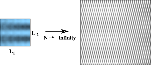
Figure 2: Noncommutative plane as a continuum and large-volume limit of noncommutative torus. The limit requires $N\rightarrow\infty$.

Start with a noncommutative torus ${\hbox to0.0pt{\cmss T\hss}\hskip 2.0pt\hbox{\cmss T}}^{2}_{\theta}$, defined through so-called quotient condition on $(N\times N)$ matrices $X^{1},X^{2}$ as:

$$X^{a}+L^{a}\delta^{a}_{b}{\hbox to0.0pt{\rm I\hss}\hskip 2.6pt\hbox{\rm I}}_{N}=\hbox{\cmsss U}_{b}^{-1}X^{a}\hbox{\cmsss U}_{b}\qquad\quad(a,b=1,2).$$

Generically, a nontrivial solution to the quotient condition requires $N\rightarrow\infty$. Applying the condition on two different directions on ${\hbox to0.0pt{\cmss T\hss}\hskip 2.0pt\hbox{\cmss T}}^{2}_{\theta}$, one finds that the quotients $\hbox{\cmsss U}_{a}$’s ought to obey

$$\hbox{\cmsss U}_{a}\hbox{\cmsss U}_{b}\,\hbox{\cmsss U}^{-1}_{a}\hbox{\cmsss U}^{-1}_{b}=e^{-i\Theta^{ab}}\,{\hbox to0.0pt{\rm I\hss}\hskip 2.6pt\hbox{\rm I}}.$$

where $\Theta_{ab}$ is dimensionless and will shortly be identified, for a square torus, with $\Theta^{ab}=\theta^{ab}(\frac{2\pi}{L})^{2},\ (L_{1}=L_{2}=L)$.

The scalar field $\bf T$ defined on ${\hbox to0.0pt{\cmss T\hss}\hskip 2.0pt\hbox{\cmss T}}^{2}_{\theta}$ is defined via

$${\bf T}=\sum_{\{{\bf m}\}={\hbox to0.0pt{\cmss Z\hss}\hskip 1.8pt\hbox{\cmss Z}}}\widetilde{\bf T}_{\bf m}\,\hbox{\cmsss U}_{1}^{m_{1}}\,\hbox{\cmsss U}_{2}^{m_{2}}.$$

Here, $\widetilde{\bf T}_{\bf m}$ belongs to a sufficiently rapidly decreasing sequence of appropriate Schwartz space.

One can represent the $\hbox{\cmsss U}_{1},\hbox{\cmsss U}_{2}$ basis in terms of Hermitian operators of the form:

$$\hbox{\cmsss U}_{a}=\exp\left(2\pi i{{\bf y}^{a}\over L^{a}}\right)\qquad\qquad(a=1,2),$$

where, in the large-$N$ limit,

$$\left[\widehat{y^{a}},\widehat{y^{b}}\right]\approx i\left({L_{a}L_{b}\over(2\pi)^{2}}\right)\Theta^{ab}\equiv i\ \theta^{ab},$$

in which we have used Eq.(2.1) in the last step.

The simplest situation arises for so-called rational noncommutative tori. For our purposes it is sufficiently general to consider, among these, the case when

$$\Theta^{ab}=\Theta\epsilon^{ab}\qquad{\rm and}\qquad\ \Theta=1/N.$$

Focusing on the square torus $L_{1}=L_{2}=L$ from now on, we get, using the above two equations,

$$\theta=\left(\frac{L}{2\pi}\right)^{2}\Theta=\left(\frac{L}{2\pi}\right)^{2}\frac{1}{N}.$$ (2.13)

For the noncommutative torus with such a value of $\theta$ , the Weyl-Moyal correspondence maps the partition function Eq.(2.12) of the NCFT on ${\hbox to0.0pt{\cmss T\hss}\hskip 2.0pt\hbox{\cmss T}}^{2}_{\theta}$ to the following partition function for a Hermitian matrix of size $(N\times N)$:

$${\hbox{\cmsss Z}}_{N}[\Theta,V;N]\,=\,\int\left[{\rm d}{\bf T}\right]_{N}\,\exp\Big{(}-{\hbox{\cmss S}\hbox to0.0pt{\hss\vrule height=8.0pt,width=0.6pt,depth=-0.1pt\hskip-4.0pt\phantom{.} }}_{{\rm NC}}[\Theta;V({\bf T})]\Big{)},$$ (2.14)

where the matrix integral measure is given by

$$\left[{\rm d}{\bf T}\right]_{N}:=\prod_{i=1}^{N}d{\bf T}_{ii}\prod_{1\leq i<j\leq N}2{\rm d}\,{\rm Re}({\bf T}_{ij}){\rm d}\,{\rm Im}({\bf T}_{ij}).$$

Let us now consider the limit $L\rightarrow\infty$; in this limit the noncommutative torus ${\hbox to0.0pt{\cmss T\hss}\hskip 2.0pt\hbox{\cmss T}}^{2}_{\theta}$ ought to approach the noncommutative plane ${\hbox{\cmss R}\hbox to0.0pt{\hss\vrule height=8.0pt,width=0.8pt,depth=-0.1pt\hskip 0.6pt\phantom{.} }}^{2}_{\theta}$. Since the Heisenberg algebra Eq.(2.1) on ${\hbox{\cmss R}\hbox to0.0pt{\hss\vrule height=8.0pt,width=0.8pt,depth=-0.1pt\hskip 0.6pt\phantom{.} }}^{2}_{\theta}$ has only infinite-dimensional representations, the above limit must also be accompanied by a limit $N\rightarrow\infty$. As $\theta\sim L^{2}/N$ (from Eq.(2.13)), the large-$\theta$ limit discussed in Sec 2.1 can be attained by

$$L\to\infty,\qquad N\to\infty,\qquad{\rm and}\qquad\theta\sim L^{2}/N\to\infty.$$

This is achievable by letting

$$L\sim N^{\gamma}\quad\Rightarrow\quad\theta\sim N^{\nu}\qquad{\rm where}\qquad\nu=(2\gamma-1),$$ (2.15)

where we assume

$$\gamma>\frac{1}{2}\quad\Rightarrow\quad\nu>0.$$

To sum up, the above observations lead to the definition of the quantum NCFT on ${\hbox{\cmss R}\hbox to0.0pt{\hss\vrule height=8.0pt,width=0.8pt,depth=-0.1pt\hskip 0.6pt\phantom{.} }}^{2}_{\theta}$ as follows:

$$\lim_{L_{1}L_{2}\rightarrow\infty}\,{\cal Z}_{\rm NC}[\theta,V_{\star};L_{1}L_{2}]\quad\equiv\quad\lim_{N\rightarrow\infty}\,\hbox{\cmsss Z}_{N}[\theta,V;N],$$

(2.16)

where, on the right-hand side, the noncommutativity parameter $\theta$ is given in terms of Eq.(2.13).

2.4 Classical, Planar, and Disordered Phases of NCFT₂

The Weyl-Moyal equivalence Eq.(2.16), together with Eq.(2.15), indicates that the quantum NCFT is actually defined in terms of a double-series expansion: large-$N$, and large-$\theta$ expansions. To detail, define the quantum NCFT in terms of the Hermitian matrix model, as in the right-hand side of Eq.(2.16). Suppose, at large $\theta$, we ignore the subleading part ${\cal L}_{-1}$ in the action Eq.(2.4). In that case, the partition function becomes identical in form to the one-matrix integral [15] and the $c<1$ matrix models for $c<1$ noncritical strings [17]. These latter models are defined in terms of the matrix model partition function ${\hbox to0.0pt{\cmss Z\hss}\hskip 1.8pt\hbox{\cmss Z}}_{\rm mm}$

$${\hbox to0.0pt{\cmss Z\hss}\hskip 1.8pt\hbox{\cmss Z}}_{\rm mm}[\beta,V;N]=\int{\rm d}{\bf M}\,\exp\Big{(}-\beta{\rm Tr}_{N}V({\bf M})\Big{)},$$ (2.17)

where $V(x)$ is the Boltzmann function, taking a polynomial form: $V(x)=a_{2}x^{2}+a_{4}x^{4}+\ldots$. Evidently, modulo the identification , $\theta=\beta$, we have

$$\hbox{\cmsss Z}_{N}[\theta,V;N]\quad=\quad{\hbox to0.0pt{\cmss Z\hss}\hskip 1.8pt\hbox{\cmss Z}}_{\rm mm}[\beta,V;N].$$ (2.18)

To investigate the partition function $\hbox{\cmsss Z}_{N}$, we will therefore proceed as in the case of the one-matrix model. Integrating out the ‘angular part’ of ${\bf T}$, the partition function $\hbox{\cmsss Z}_{N}$ is rewritable as an integral over the $N$ eigenvalues $\lambda_{1},\lambda_{2},\cdots,\lambda_{N}$ of ${\bf T}$ [15]:

$$\hbox{\cmsss Z}_{N}[\theta,V;N] = C_{N}\int\prod_{k=1}^{N}{\rm d}\lambda_{k}\prod_{k<\ell}^{N}(\lambda_{k}-\lambda_{\ell})^{2}\,\exp\Big{(}-{\rm}\theta\sum_{k}V(\lambda_{k})\Big{)}$$ (2.19)

$$= C_{N}\int\prod_{k=1}^{N}{\rm d}\lambda_{k}\exp\Big{(}-S_{\rm eff}(\lambda_{1},\cdots,\lambda_{N})\Big{)},$$

where

$$C_{N}={\rm Vol}\left[{{\rm U}(N)\over{{\rm U}(1)}^{N}\times{\cal S}_{N}}\right]={1\over N!}\prod_{K=1}^{N}{(2\pi)^{K-1}\over\Gamma(K)}$$

refers to the angular volume measure factor, and

$$S_{\rm eff}(\lambda_{1},\cdots,\lambda_{N})\,\,=\,\,S_{\rm classical}[N,\theta]\,+\,S_{\rm measure}[N]$$ (2.20)

with

$$S_{\rm classical}[N,\theta]=N{\rm}\theta\left({1\over N}\!\!\sum_{k=1}^{N}V(\lambda_{k})\right)\qquad{\rm and}\qquad S_{\rm measure}[N]=N^{2}\left({1\over 2N^{2}}\!\!\!\sum_{1\leq k\neq\ell\leq N}\ln(\lambda_{k}-\lambda_{\ell})^{2}\right)$$

refers to the effective action as a sum of the classical contribution and the measure factor contribution.

The large-$N$ limit of one-matrix models are describable by a master field configuration, where distribution of the eigenvalues $\lambda_{1},\cdots,\lambda_{N}$ are encoded into the density field $\rho(\lambda)$, introduced in Eq.(2.7), with support over connected compact domains ${\cal D}$ and subject to the constraints:

$$\int_{\cal D}{\rm d}\lambda\rho(\lambda)=1\qquad\quad{\rm and}\quad\qquad\rho(\lambda)\geq 0\quad{\rm on}\quad\lambda\subset{\cal D}.$$ (2.21)

The effective action of eigenvalues then become

$$S_{\rm eff}[\rho]=N^{2}\left[g^{-2}_{\rm eff}\int_{\cal D}\!{\rm d}\lambda\,\rho(\lambda)V(\lambda)-\int_{\cal D}\!{\rm d}\lambda\!\int_{{\cal D}}\!{\rm d}\mu\,\rho(\lambda)\Big{(}\ln|\lambda-\mu|\Big{)}\rho(\mu)\right],$$ (2.22)

in which

$$g^{2}_{\rm eff}\equiv{N\over{\rm}\theta}$$ (2.23)

measures the relative weight between the classical contribution and the measure factor contribution.

Now the effective action Eq.(2.22) is exactly of the form as Eq.(1.1). One thus discovers that, in quantum NCFT, there ought to exist three distinct regimes as in Eq.(1.2). If one were to define the quantum NCFT in terms of the Hermitian matrix model, as in Eq.(2.16), via Weyl-Moyal equivalence, the three different regimes are distinguished by relative weight in Eq.(2.22) between the classical contribution $S_{\rm classical}\sim{\cal O}(N{\rm}\theta)$ and the matrix-integral measure part contribution $S_{\rm measure}\sim{\cal O}(N^{2})$.

The above considerations entail an important consequence to the interpretation of the noncommutative field theories and the classical solutions therein, as studied in [3]. First, in noncommutative field theory, one defines the theory by viewing noncommutative field ${{\rm T}}$ as a representation of the Heisenberg algebra, which is infinite-dimensional in case the theory is defined on ${\hbox{\cmss R}\hbox to0.0pt{\hss\vrule height=8.0pt,width=0.8pt,depth=-0.1pt\hskip 0.6pt\phantom{.} }}^{2}_{\theta}$. If one interprets this as meaning that the size $N$ of the matrix-field ${\bf T}$ is strictly infinite to begin with, then the classical action $S_{\rm classical}$ becomes insignificant, as it is far outweighted by the quantum contribution $S_{\rm measure}$ coming from the matrix-interal measure. Second, in order to be able to view the classical solutions, e.g. solutions studied in [3], as saddle-points of the partition function Eq.(2.12), one must first ‘regulate’ the noncommutative field theory in such a way that the corresponding Weyl formulation is defined on a finite $N$-dimensional Hilbert space to begin with, viz. the Hermitian matrix model is for $(N\times N)$ matrices. In order to recover a sensible saddle-point solution, one subsequently needs to take an appropriate large-$\theta$, large-$N$ limit. Eq.(1.2) indicates that, a priori, there are three types of possible scaling of the noncommutative field theory. Based on this observation, we thus conclude that, only in the classical scaling (a), the classical solutions found in [3] are also the saddle-point solutions. For the planar scaling (b), the classical solutions ought to be replaced, as we will find in the next section, by new ones in which the eigenvalues are distributed. In the quantum scaling (c), the classical solutions found in [3] are washed out completely.

2.5 Quantum Vacua and Instantons

We now flesh up the preceding discussion by studying the quantum vacua and instantons of the two-dimensional NCFT on ${\hbox{\cmss R}\hbox to0.0pt{\hss\vrule height=8.0pt,width=0.8pt,depth=-0.1pt\hskip 0.6pt\phantom{.} }}^{2}_{\theta}$ in the large-$N$, large-$\theta$ limit in the various regimes Eq.(1.2). In doing so, we will use the analogy Eq.(2.18) with the one-matrix model studied in the context of $c<1$ noncritical string [17] to quantize the solutions described in Sec 2.2. We will do explicit calculations in the GMS- and planar-phases and will make some qualitative remarks about the disordered phase.

We begin by defining the ‘free’energy $F[\theta,V;N]$ as:

$$\hbox{\cmsss Z}_{N}[\theta,V;N]:=\left({2\pi\over N}\right)^{N^{2}/2}\,e^{-F[\theta,V;N]},$$

where the normalization is chosen so that $F=0$ for quadratic potential $V({\bf T})={1\over 2}{\rm Tr}{\bf T}^{2}$. As is well-known [15], the free energy has the following large-$N$ expansion:

$$F[\theta=(N/g_{\rm eff}^{2}),N]=N^{2}F_{0}(g^{2}_{\rm eff})+F_{1}(g^{2}_{\rm eff})+N^{-2}F_{2}(g^{2}_{\rm eff})+\ldots,$$ (2.24)

where each of the $F_{n}$ are defined via power series in $g^{2}_{\rm eff}$ with a radius of convergence $g_{c}$. It will be convenient at this stage to rephrase the three limits Eq.(1.2) as

$$\begin{array}[]{cccc}{\rm(a)}\hskip 14.22636pt&{\rm GMS~{}~{}phase}:&\hskip 14.22636ptN\to\infty,&\ \hskip 14.22636ptg_{\rm eff}\to 0\\ {\rm(b)}\hskip 14.22636pt&{\rm planar~{}~{}phase}:&\hskip 14.22636ptN\to\infty,&\ \hskip 26.17648ptg_{\rm eff}={\rm fixed}\\ {\rm(c)}\hskip 14.22636pt&{\rm disordered~{}~{}phase}:&\hskip 14.22636ptN\to\infty,&\ \hskip 18.49411ptg_{\rm eff}\to\infty.\end{array}$$ (2.28)

The leading term $F_{0}$ in Eq.(2.24) is given by the saddle-point contribution at large-$N$ limit. Clearly, the leading behavior of (a) the GMS-phase free energy, and (b) the planar-phase free energy (for $g_{\rm eff}<g_{c}$) are derivable from this saddle-point expression. The disordered phase free energy is clearly in the strong coupling phase $g_{\rm eff}>g_{c}$ in which the large-$N$ expansion Eq.(2.24) breaks down.

We see, therefore, that we can derive the leading behaviour of the partition function $\hbox{\cmsss Z}_{N}$ in the double limit, $N\to\infty,\theta\to\infty$, from the large-$N$ saddle-point (except in the disordered phase). We describe in Appendix B how to compute the large-$N$ saddle-point as minima of the effective action Eq.(2.22) subject to the constraint Eq.(2.21). We simply quote the result here (see Appendix B or [15, 24] for more details of the derivation).

For the double-well potential of the type Eq.(2.8), the saddle-point density is given in terms of two-cut eigenvalue distribution :

$$\rho_{{\rm s}}(\lambda)\,\,=\left\{\begin{array}[]{ccc}{1\over 2}g^{-2}_{\rm eff}\,\sqrt{\lambda^{2}\Big{(}\lambda^{2}-\lambda_{-}^{2}\Big{)}\Big{(}\lambda_{+}^{2}-\lambda^{2}\Big{)}}&\qquad{\rm for}&\lambda\in(-\lambda_{+},-\lambda_{-})\cup(\lambda_{-},\lambda_{+}),\\ &&\\ \qquad 0&{\rm otherwise}.&\end{array}\right.$$ (2.32)

Here,

$$\lambda_{-}=\sqrt{\Big{(}{\rm T}_{0}-2g^{2}_{\rm eff}\Big{)}},\qquad\quad\lambda_{+}=\sqrt{\Big{(}{\rm T}_{0}+2g^{2}_{\rm eff}\Big{)}}.$$

As explained above, Eq.(2.32) is the leading large-$N$, large-$\theta$ value of the quantum corrected density function, in the planar limit (b), corresponding to the classical $(N_{1},N_{2})$ instanton of Sec 2.2 for $N_{1}=N_{2}$.

Eq.(2.32) is clearly different from the classical (GMS) value (Eq.(2.11) with $N_{1}=N_{2}$). But from what we have discussed above, we expect to recover the classical (GMS) value in the weak ‘t Hooft coupling limit, $g_{\rm eff}\rightarrow 0$. This is indeed what happens. In this limit, the eigenvalue density, Eq.(2.32), reduces to

$$\rho_{\rm s}(\lambda)\,\,\longrightarrow\,\,\rho_{\rm classical}(\lambda)={\frac{1}{2}}\delta(\lambda-{\rm T}_{0})+{\frac{1}{2}}\delta(\lambda+{\rm T}_{0}).$$

This is identical with Eq.(2.11) for

$$N_{1}=N_{2}={\frac{N}{2}}\qquad{\rm equivalently}\qquad n_{1}=n_{2}={\frac{1}{2}}.$$

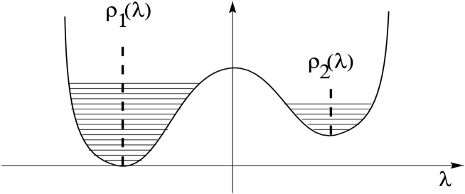
Figure 3: Eigenvalue distributions for noncommutative vacua and instantons. Classically, the eigenvalues are piled up to delta-function type distribution, as depicted as the dashed line. Quantum mechanically, the eigenvalues repel each other and are spread over, as depicted by the horizontal lines.

It is worth mentioning that, for the scaling (b), the classical limit $g_{\rm eff}\rightarrow 0$ of the planar saddle-point configuration is not necessarily the same as the classical regime (a). As the result Eq.(2.32) for the double-well potential exemplifies, the ‘classical limit’ $g_{\rm eff}\rightarrow 0$ yields, out of $N$ possible classical instantons of type $(N_{1},N_{2})$, the one with $N_{1}=N_{2}=N/2$ singled out.

In fact, it is possible to visualize the quantum instantons as non-interacting quantum vacua, localized at $\lambda_{-}$ and $\lambda_{+}$, respectively. Consider the situation that the two potential wells are widely separated and contain $N_{1},N_{2}$ eigenvalues, respectively. Then, the partition function reads

$$\hbox{\cmsss Z}[\theta,V;n_{1},n_{2}]=\int_{-\infty}^{\Lambda}\!\prod_{k=1}^{N_{1}}{\rm d}\lambda_{k}\int_{\Lambda}^{+\infty}\!\!\prod_{\ell=N_{1}}^{N}{\rm d}\lambda_{\ell}\,\prod_{1\leq k<\ell\leq N}(\lambda_{k}-\lambda_{\ell})^{2}\,\exp\Big{(}-{\hbox{\cmss S}\hbox to0.0pt{\hss\vrule height=8.0pt,width=0.6pt,depth=-0.1pt\hskip-4.0pt\phantom{.} }}_{\rm NC}[\theta,V;N_{1},N_{2}]\Big{)}.$$

Here, $\Lambda$ denotes a suitably chosen, midpoint ‘cutoff’ value of the eigenvalue between the two cuts. In fact, the above partition function is expressible as a matrix integral over two separate matrices: ${\bf T}_{1}$ of size $(N_{1}\times N_{1})$ and ${\bf T}_{2}$ of size $(N_{2}\times N_{2})$, whose eigenvalues are restricted to be less than or larger than $\Lambda$, respectively. One easily finds that:

$$\hbox{\cmsss Z}[\theta,V;n_{1},n_{2}]=\int[{\rm d}{\bf T}_{1}]_{N_{1}}\int[{\rm d}{\bf T}_{2}]_{N_{2}}\,\exp\Big{(}-{\hbox{\cmss S}\hbox to0.0pt{\hss\vrule height=8.0pt,width=0.6pt,depth=-0.1pt\hskip-4.0pt\phantom{.} }}_{\rm NC}[\theta,V;N_{1},N_{2}]\Big{)},$$

where

$${\hbox{\cmss S}\hbox to0.0pt{\hss\vrule height=8.0pt,width=0.6pt,depth=-0.1pt\hskip-4.0pt\phantom{.} }}_{\rm NC} = {\rm}\theta\,\left[{\rm Tr}V({\bf T}_{1})+{\rm Tr}V({\bf T}_{2})\right]$$ (2.33)

$$+ \left[2{\rm Tr}\left(\ln({\bf T}_{1}\otimes{\hbox to0.0pt{\rm I\hss}\hskip 2.6pt\hbox{\rm I}}-{\hbox to0.0pt{\rm I\hss}\hskip 2.6pt\hbox{\rm I}}\otimes{\bf T}_{2})\right)+\cdots\right],$$

in which the ellipses denote gradient corrections. The above effective two-matrix integral is well-defined in the large-$N$, large-$\theta$ limit. Evidently, at leading-order in $(1/\theta)$-expansion, the matrix intergral is factorized into two disjoint one-matrix integrals, except that the eigenvalues are bounded from above and below, respectively. The saddle-point configuration is described precisely by the above solution. The error involed in ellipses in Eq.(2.33) is of order $e^{-{\cal O}(N)}$, due to tunnelling effect, and hence is completely negligible in the continuum limit.

2.6 Quantum Corrections

The central observation in the foregoing discussion was that the quantum effects drive the eigenvalues to repel each other — dramatic change when compared to the situation at classical level. To demonstrate how striking the quantum effects are, let us compute the ‘quantum’ Euclidean action and compare its ground-state value with that of classical action. The second-order perturbation theory asserts that, around the ground-state, quantum corrections to physical quantities are typically negative. Thus, one would expect that, once the quantum corrections are taken into account, the Euclidean action gets lowered. In quantum NCFT, quite to the contrary, we will find that the quantum effects increase the Euclidean action! This has to do with the fact that the repulsion among eigenvalues is a purely quantum-mechanical effect, not present at classical level at all.

Begin with the effective action of the eigenvalue density field, $\rho(\lambda)$, Eq.(2.22). The saddle-point configuration is governed by solutions of Eq.(B.2). We shall be taking a generic condition that the classical potential $V(\lambda)$ is a concave function of $\lambda$ with a global minimum at $\lambda=\lambda_{\rm s}$ and denote $V(\lambda_{\rm s})=V_{0}$. Evidently, $V(\lambda)\geq V_{0}$ for all $\lambda$. Multiplying Eq.(B.2) with $\rho_{\rm s}(\lambda)$ and then integrating over $\lambda$, we obtain

$$N^{2}\left[g^{-2}_{\rm eff}\int_{\cal D}{\rm d}\lambda\rho_{\rm s}(\lambda)V(\lambda)-2\int{\rm d}\mu{\rm d}\lambda\,\rho_{\rm s}(\mu)\ln|\lambda-\mu|\rho_{\rm s}(\lambda)\right]=N\theta E,$$

where we have used the normalization condition, $\int{\rm d}\lambda\,\rho_{\rm s}(\lambda)=1$ and $E$ is the first-integral of motion. Using this relation, the quantum Euclidean action Eq.(2.22) is re-expressible as:

$$S_{\rm eff}[\rho_{\rm s}] = N^{2}\left[g^{-2}_{\rm eff}\int_{\cal D}{\rm d}\lambda\rho_{\rm s}(\lambda)V(\lambda)-\int_{\cal D}{\rm d}\lambda\int_{\cal D}{\rm d}\mu\,\rho_{\rm s}(\lambda)\ln|\lambda-\mu|\rho_{\rm s}(\mu)\right]$$ (2.34)

$$= N\theta E+{1\over 2}N\theta\left(\int{\rm d}\lambda\rho_{\rm s}(\lambda)V(\lambda)-E\right).$$

The first-integral of motion $E$ is fixed uniquely to $E=N{\rm}\theta\,V_{0}$ by demanding that, in the weak ‘t Hooft coupling limit, $g_{\rm eff}\rightarrow 0$, the saddle-point value of the quantum Euclidean action Eq.(2.34) reduces to that of the classical Euclidean action, $S_{\rm classical}=N{\rm}\theta\,V_{0}$. Thus, one readily finds that the second term in Eq.(2.34) amounts to change of the Euclidean action due to quantum effects.

Let us now evaluate the second term in Eq.(2.34), the quantum correction to the Euclidean action. First of all, from the expression, whether the correction is negative – as the second-order perturbation theory suggests – or not is easily analyzable. Classically, the $N$ species of eigenvalues were all sitting at a single point $\lambda=\lambda_{\rm s}$, but, once the quantum effects are taken into account, they will repel each other and form a domain, denoted in Eq.(2.34) as ${\cal D}$, of eigenvalue distribution around the point $\lambda=\lambda_{\rm s}$. Take a generic point $\lambda$ inside ${\cal D}$. As $V(\lambda)\geq V_{0}$ by the definition of $\lambda_{\rm s}$ and $\rho_{\rm s}(\lambda)$ is distributed over ${\cal D}$, it follows immediately that

$$\Delta E := \left(S_{\rm eff}-N\theta E\right)$$

$$= {1\over 2}N{\rm}\theta\left(\int_{\cal D}{\rm d}\lambda\,\rho_{\rm s}(\lambda)V(\lambda)-E\right)$$

$$= {1\over 2}N{\rm}\theta\int_{\cal D}{\rm d}\lambda\,\rho_{\rm s}(\lambda)\Big{(}V(\lambda)-V_{0}\Big{)}$$

$$\geq 0.$$

This proves that the quantum correction in Eq.(2.34) is positive, in contrast to what one expects from the second-order perturbation theory. Evidently, the reason has to do with eigenvalue repulsion — classically invisible but quantum-mechanically generated effect. The repulsion gives rise to a positive ‘pressure’, resulting in increase of the Euclidean action.

We now compute the increment of the Euclidean action explicitly. We will take, for simplicity, $V(\lambda)={1\over 2}\lambda^{2}$ — an approximation applicable, at leading-order, for each cut of a generic concave potential, according to the result of Eq.(2.33). Utilizing Eq.(B.3) (see also [15]), it is straightforward to compute $\rho_{\rm s}(\lambda)$. We find

$$\rho_{\rm s}(\lambda)={1\over 2\pi}\sqrt{4-\lambda^{2}}\,\,\qquad{\rm for}\qquad-2\leq\lambda\leq+2.$$ (2.36)

Substituting Eq.(2.36) into Eq.(2.6), we obtain (recall that here the classical energy is normalized as $N\theta E=0$)

$$\Delta E=S_{\rm eff}[\rho_{\rm s}] = N{\rm}\theta\int_{0}^{2}{\rm d}\lambda{1\over 2\pi}\sqrt{4-\lambda^{2}}\cdot{1\over 2}\lambda^{2}$$

$$= \frac{1}{4}N\theta.$$

Thus, the correction is of order $N^{2}$ in the planar-phase (b) of Eq.(2.28).

We conclude this section by mentioning that quantum corrections in the disordered phase cannot be calculated by the above procedure, as the large-$N$ saddle-point is irrelevant. It is readily seen, however, that the quantum corrections in the disordered phase will be larger. In the example analyzed below, we will see that $(\Delta E)_{\rm Q}/(\Delta E)_{\rm planar}\to\infty$ in the disordered phase (c) of Eq.(1.2).

2.7 Perturbative Manifestation of the Vandermonde Effect

The effect of $S_{\rm measure}$ in Eq.(2.20), being originated from the vandermonde determinant of the functional integral measure, ought to be obtainable in the standard Feynman diagrammatics. How does the effects manifest themselves? We will now show that, in the context of the Feynman diagrammatics in Weyl formulation, the aforementioned limits Eq.(1.2) or Eq.(2.28) is derivable at large-$\theta$ and large-$L$ limit .

Begin with Feynman rules defined in the Moyal formulation by Eq.(2.12) and the potential Eq.(2.8). Our objective is to see how the quantum corrections differ in the three scaling regimes, Eq.(1.2). In computing the effects, we keep in mind the relations Eq.(2.13) between the parameters $(L,\theta)$ of ${{\hbox to0.0pt{\cmss T\hss}\hskip 2.0pt\hbox{\cmss T}}^{2}_{\theta}}$ and the parameters $(N,\theta)$ of ${{\hbox{\cmss R}\hbox to0.0pt{\hss\vrule height=8.0pt,width=0.8pt,depth=-0.1pt\hskip 0.6pt\phantom{.} }}^{2}_{\theta}}$.

Expand the action around the ‘right vacuum’ ${\rm T}({\bf x})={\rm T}_{0}+\phi({\bf x})$:

$$S_{\rm NC}=\theta\int{\rm d}^{2}{\bf x}\left[V_{0}+\left(\lambda_{4}{\rm T}_{0}^{2}\phi^{2}+\lambda_{4}{\rm T}_{0}\phi^{3}+{\lambda_{4}\over 4}\phi^{4}\right)+\left(-{1\over 2\theta}\left(\partial_{\bf x}\phi\right)^{2}\right)\right]_{\star}.$$ (2.37)

Consider, for definiteness, the nonplanar, one-loop contribution to the connected two-point Green function, depicted in Fig.(4). This diagram provides an example of IR problems in NCFT[21].

Figure 4: one-loop, non-planar contribution to two-point Green function.

The contribution involves the following moduli-space integral associated with one-loop Feynman diagram, where $D$ denotes the spacetime dimension:

$$I_{D}=\int\limits_{0}^{\infty}{\rm d}t{1\over t^{D/2}}\exp\left(-tm^{2}-{\Lambda_{\rm eff}^{2}\over t}\right),$$

where $m^{2}=2$ from Eq.(2.37), ${\bf p}$ is the momentum flow through the external line, and

$$\Lambda_{\rm eff}^{-2}=\Lambda_{\rm UV}^{-2}+2\lambda_{4}\left(\theta\cdot{\bf p}\right)^{2}.$$

The result is

$$I_{2} = 2K_{0}\left({2m}/{\Lambda}_{\rm eff}\right)\rightarrow\log\left({2m}/{\Lambda}_{\rm eff}\right)+\ldots\qquad{\rm for}\qquad\left({2m}/{\Lambda_{\rm eff}}\right)\ll 1$$

$$\rightarrow 2K_{0}\left(2m|\theta{\bf p}|\right)\qquad\qquad\qquad\qquad\qquad{\rm for}\qquad{\bf p}={\rm finite},\quad\Lambda\rightarrow\infty$$

$$\sim 2K_{0}\left(2m\theta/L\right)\qquad\qquad\qquad\qquad\qquad{\rm for}\qquad|{\bf p}|\sim 1/L.$$

Using the relation $L=\sqrt{\theta N}$ on ${\hbox to0.0pt{\cmss T\hss}\hskip 2.0pt\hbox{\cmss T}}^{2}_{\theta}$, we finally obtain

$$I_{2}=2K_{0}\left({2m\over g_{\rm eff}}\right).$$

Thus, $I_{2}=\infty$ in the disordered phase, $I_{2}=$ finite in the planar phase, and $I_{2}=0$ in the GMS phase. This is exactly as we would predict on the basis of our earlier discussion of the behaviour of the quantum effective action in the limits Eq.(1.2), namely that the GMS solution remains stable in the limit (a), has a finite correction in the planar limit (b), and is completely destabilized in the limit (c), where the measure term becomes infinitely large compared to the classical term in the action.

3 Effect of the Gradient Term

The foregoing discussion was largely based on keeping only the leading order term, ${\cal L}_{0}$ in Eq.(2.5), at large ${\rm}\theta$ limit. While the gradient-term ${\cal L}_{-1}$ is sub-leading order in $(1/{\rm}\theta)$-expansion, as noted below Eq.(A.4), it breaks the U($\infty$) symmetry explicitly — a point which ought to be concerned for its consequential effects to the results we have obtained in the previous subsections. In particular, as the dramatic quantum effects we have deduced are largely based on ${\cal L}_{0}$-term and U($\infty$) symmetry therein, one might suspect that the term ${\cal L}_{-1}$, being part of the classical action, would render a sizable symmetry breaking effect. This is because the size of the gradient-term is given by

$${\hbox{\cmss S}\hbox to0.0pt{\hss\vrule height=8.0pt,width=0.6pt,depth=-0.1pt\hskip-4.0pt\phantom{.} }}_{-1}=\int{\rm d}^{2}{\bf x}{\cal L}_{-1}=\int{\rm d}^{2}{\bf x}\left(-{1\over 2}[{\bf x},{\rm T}]_{\star}^{2}\right)\quad\sim\quad{\cal O}(N^{2}).$$

Fortuitously, as we will show in this section, the gradient effect turns out to be of order ${\cal O}(N^{2}g_{\rm eff}^{2})$, viz. scales further by a factor of the ‘t Hooft coupling, $g^{2}_{\rm eff}$. The scaling is not universally valid, but only for $g_{\rm eff}<g^{\rm c}_{\rm eff}$ for some finite $g^{c}_{\rm eff}$, as is inferred from the large-$N$ phase transition [26]. As we are interested in the weak ‘t Hooft coupling regime, $g_{\rm eff}\ll 1$, the above counting holds valid. In particular, it implies that the measure effect, whose size is of order ${\cal O}(N^{2})$, outweighs the gradient effect. Thus, in the weak ‘t Hooft coupling regime, one can utilize the U$(\infty)$ symmetry, and recast the NCFTs literally as the $N\rightarrow\infty$ limit of the matrix model studied in [15].

3.1 Perturbative Estimates

We will begin with, utilizing the Weyl formulation of the NCFT, computation of leading-order perturbative corrections. For this purpose, we regularize the theory so that fields are defined on $N$-dimensional Hilbert space, ${\cal H}_{\theta}[N]$, spanned by Span[$|n\rangle,n=0,\ldots,N-1$], where

$$|n\rangle=\frac{a^{\dagger n}}{\sqrt{n!}}|0\rangle\qquad{\rm and}\qquad\frac{1}{\sqrt{2}}[\widehat{{\bf x}^{1}}\pm i\widehat{{\bf x}^{2}}]\equiv({\bf a},{\bf a}^{\dagger}).$$

Taking the potential as Eq.(2.8) and expanding around ${\bf T}=0$, the NCFT partition function Eq.(2.14) is given by

$$\hbox{\cmsss Z}_{N}=\int[{\rm d}{\bf T}]_{N}\exp\left(-{\hbox{\cmss S}\hbox to0.0pt{\hss\vrule height=8.0pt,width=0.6pt,depth=-0.1pt\hskip-4.0pt\phantom{.} }}_{\rm NC}[\theta;{\bf T}]\right),\qquad{\rm where}\qquad{\hbox{\cmss S}\hbox to0.0pt{\hss\vrule height=8.0pt,width=0.6pt,depth=-0.1pt\hskip-4.0pt\phantom{.} }}_{\rm NC}=\Big{(}{\hbox{\cmss S}\hbox to0.0pt{\hss\vrule height=8.0pt,width=0.6pt,depth=-0.1pt\hskip-4.0pt\phantom{.} }}_{\rm cl}+{\hbox{\cmss S}\hbox to0.0pt{\hss\vrule height=8.0pt,width=0.6pt,depth=-0.1pt\hskip-4.0pt\phantom{.} }}_{\rm 0P}+{\hbox{\cmss S}\hbox to0.0pt{\hss\vrule height=8.0pt,width=0.6pt,depth=-0.1pt\hskip-4.0pt\phantom{.} }}_{\rm 0V}\Big{)}+{\hbox{\cmss S}\hbox to0.0pt{\hss\vrule height=8.0pt,width=0.6pt,depth=-0.1pt\hskip-4.0pt\phantom{.} }}_{-1}.$$

Here,

$${\hbox{\cmss S}\hbox to0.0pt{\hss\vrule height=8.0pt,width=0.6pt,depth=-0.1pt\hskip-4.0pt\phantom{.} }}_{\rm cl} = \theta{\rm Tr}V(0)\,\,\qquad\qquad{\rm where}\qquad V(0)=V_{0}+{\lambda_{4}\over 4}{\rm T}_{0}^{4}$$

$${\hbox{\cmss S}\hbox to0.0pt{\hss\vrule height=8.0pt,width=0.6pt,depth=-0.1pt\hskip-4.0pt\phantom{.} }}_{\rm 0P} = \theta{\rm Tr}\left({m^{2}\over 2}{\bf T}^{2}\right)\qquad{\rm where}\qquad m^{2}={\lambda_{4}\over 2}{\rm T}^{2}_{0}$$

$${\hbox{\cmss S}\hbox to0.0pt{\hss\vrule height=8.0pt,width=0.6pt,depth=-0.1pt\hskip-4.0pt\phantom{.} }}_{\rm 0V} = \theta{\rm Tr}\left({\lambda_{4}\over 4}{\bf T}^{4}\right)$$

$${\hbox{\cmss S}\hbox to0.0pt{\hss\vrule height=8.0pt,width=0.6pt,depth=-0.1pt\hskip-4.0pt\phantom{.} }}_{-1} = {\rm Tr}\left(-\frac{1}{2}\left[\widehat{\bf x},{\bf T}\right]^{2}\right).$$ (3.1)

3.2 Leading-Order Corrections

The leading-order, quantum corrections to the free energy are obtained as

$$\Big{<}{\hbox{\cmss S}\hbox to0.0pt{\hss\vrule height=8.0pt,width=0.6pt,depth=-0.1pt\hskip-4.0pt\phantom{.} }}({\bf T})\Big{>}_{\rm 0P}=\frac{1}{\hbox{\cmsss Z}_{\rm 0P}}\int[{\rm d}{\bf T}]{\hbox{\cmss S}\hbox to0.0pt{\hss\vrule height=8.0pt,width=0.6pt,depth=-0.1pt\hskip-4.0pt\phantom{.} }}({\bf T})\exp\Big{(}-{\hbox{\cmss S}\hbox to0.0pt{\hss\vrule height=8.0pt,width=0.6pt,depth=-0.1pt\hskip-4.0pt\phantom{.} }}_{\rm 0P}\Big{)}={\hbox{\cmss S}\hbox to0.0pt{\hss\vrule height=8.0pt,width=0.6pt,depth=-0.1pt\hskip-4.0pt\phantom{.} }}_{\rm cl}+\Delta{\hbox{\cmss S}\hbox to0.0pt{\hss\vrule height=8.0pt,width=0.6pt,depth=-0.1pt\hskip-4.0pt\phantom{.} }}_{\rm 0P}+\Delta{\hbox{\cmss S}\hbox to0.0pt{\hss\vrule height=8.0pt,width=0.6pt,depth=-0.1pt\hskip-4.0pt\phantom{.} }}_{\rm 0V}+\Delta{\hbox{\cmss S}\hbox to0.0pt{\hss\vrule height=8.0pt,width=0.6pt,depth=-0.1pt\hskip-4.0pt\phantom{.} }}_{-1}+\ldots$$ (3.2)

where $\hbox{\cmsss Z}_{\rm 0P}:=\int[{\rm d}{\bf T}]\exp\Big{(}-{\hbox{\cmss S}\hbox to0.0pt{\hss\vrule height=8.0pt,width=0.6pt,depth=-0.1pt\hskip-4.0pt\phantom{.} }}_{\rm 0P}\Big{)}$ and

$${\hbox{\cmss S}\hbox to0.0pt{\hss\vrule height=8.0pt,width=0.6pt,depth=-0.1pt\hskip-4.0pt\phantom{.} }}_{\rm cl} \equiv \theta{\rm Tr}V(0)\sim\theta NV(0),\qquad\qquad\quad\Delta{\hbox{\cmss S}\hbox to0.0pt{\hss\vrule height=8.0pt,width=0.6pt,depth=-0.1pt\hskip-4.0pt\phantom{.} }}_{\rm 0P}\equiv\theta m^{2}\ \Big{<}{\rm Tr}{\bf T}^{2}\Big{>}_{\rm 0P}\sim N^{2}$$

$$\Delta{\hbox{\cmss S}\hbox to0.0pt{\hss\vrule height=8.0pt,width=0.6pt,depth=-0.1pt\hskip-4.0pt\phantom{.} }}_{\rm 0V} \equiv \Big{<}{\hbox{\cmss S}\hbox to0.0pt{\hss\vrule height=8.0pt,width=0.6pt,depth=-0.1pt\hskip-4.0pt\phantom{.} }}_{\rm 0V}\Big{>}_{\rm 0P}=\theta\lambda_{4}\cdot\frac{N^{3}}{(\theta m^{2})^{2}},\qquad\quad\Delta{\hbox{\cmss S}\hbox to0.0pt{\hss\vrule height=8.0pt,width=0.6pt,depth=-0.1pt\hskip-4.0pt\phantom{.} }}_{-1}\equiv\Big{<}{\hbox{\cmss S}\hbox to0.0pt{\hss\vrule height=8.0pt,width=0.6pt,depth=-0.1pt\hskip-4.0pt\phantom{.} }}_{-1}\Big{>}_{\rm 0P}=\frac{N\cdot N^{2}}{\theta m^{2}}.$$ (3.3)

Figure 5: Feynman diagrams for leading-order quantum corrections due to (a) potential $S_{0V}$, and (b) the gradient term $S_{-1}$.

Diagrammatically, $\Delta{\hbox{\cmss S}\hbox to0.0pt{\hss\vrule height=8.0pt,width=0.6pt,depth=-0.1pt\hskip-4.0pt\phantom{.} }}_{\rm 0P}$ originates from the one-loop vacuum diagram, while $\Delta{\hbox{\cmss S}\hbox to0.0pt{\hss\vrule height=8.0pt,width=0.6pt,depth=-0.1pt\hskip-4.0pt\phantom{.} }}_{\rm 0V}$ and $\Delta{\hbox{\cmss S}\hbox to0.0pt{\hss\vrule height=8.0pt,width=0.6pt,depth=-0.1pt\hskip-4.0pt\phantom{.} }}_{-1}$ are from the diagrams (a) and (b) in Fig.(5), respectively. Note that the propagator is given by $\Big{<}{\bf T}{\bf T}\Big{>}_{\rm 0P}\sim 1/(\theta m^{2})$. Thus, the diagrams are evaluated as follows. For diagram (a), the contribution equals to (vertex) $[\theta\lambda_{4}]\times$ (two  propagators) $[1/(\theta m^{2})^{2}]\times$ (three ‘color’ loops) $[N^{3}]$. In evaluating $\Big{<}{\hbox{\cmss S}\hbox to0.0pt{\hss\vrule height=8.0pt,width=0.6pt,depth=-0.1pt\hskip-4.0pt\phantom{.} }}_{-1}\Big{>}_{\rm 0P}$, two terms will contribute: ${\rm Tr}\left({\bf T}\hat{\bf x}_{a}{\bf T}\hat{\bf x}_{a}\right)$ and ${\rm Tr}\left({\bf T}^{2}\hat{\bf x}^{2}_{a}\right)$. As ${\rm Tr}\hat{\bf x}_{a}=0$, only the latter will contribute, and is given by the Feynman diagram (b) in Fig.(5). There, ${\rm X}^{2}$ on the outer colour loop refers to the insertion of the ${\rm Tr}\left(\widehat{\bf x}_{a}^{2}\right)\sim\sum_{n=0}^{N-1}\,n={\cal O}(N^{2})$. Hence, for diagram (b), the contribution equals to (color loop) $[N]\times$ (color loop with ${\rm X}^{2}$ insertion) $[N^{2}]\times$ (one propagator) [$1/(\theta m^{2})]$.

To proceed further, introduce the following rescaled parameters:

$$\overline{\lambda_{4}}:=\frac{\lambda_{4}}{m^{2}},\qquad\overline{V}(0):=\frac{V(0)}{m^{2}},\qquad\overline{\theta}:=\frac{m^{2}\theta}{N}={m^{2}\over g^{2}_{\rm eff}}.$$

Making, in Eq.(3.1), a change of the variable $\theta m^{2}{\bf T}^{2}={\bf M}^{2}$ and bringing the quadratic term into a canonical normalization, we have

$${\hbox{\cmss S}\hbox to0.0pt{\hss\vrule height=8.0pt,width=0.6pt,depth=-0.1pt\hskip-4.0pt\phantom{.} }}_{\rm NC}=N^{2}\overline{\theta}\overline{V}(0)+{\rm Tr}\left[\ {1\over 2}{\bf M}^{2}+{1\over N}\frac{\overline{\lambda_{4}}}{\overline{\theta}}\left({1\over 4}{\bf M}^{4}\right)+{1\over N}\frac{1}{\overline{\theta}}\left(-{1\over 2}[\widehat{\bf x}_{a},{\bf M}]^{2}\right)\right],$$ (3.4)

with which the partition function Eq.(2.17) can be defined. The Eq.(3.4) reveals that the effective coupling of the potential term is $(\overline{\lambda_{4}}/\overline{\theta})$ and that of the gradient term is $\frac{1}{\overline{\theta}}$. For the perturbation theory to make sense, one will need these couplings to be small enough. We now ask if there is a range of parameters satisfying this restriction as well as the condition that the gradient terms are suppressed compared to the potential term. There indeed does exist such a region in the space of the rescaled parameters, viz.

$$\overline{\theta}\,\gg\,\overline{\lambda_{4}}\,\gg\,1.$$ (3.5)

We will now explicitly verify that, in this weak coupling regime, the gradient term is suppressed, at least at leading order in the perturbation theory. In terms of the rescaled parameters, the estimates Eq.(3.3) are re-expressible as

$${\hbox{\cmss S}\hbox to0.0pt{\hss\vrule height=8.0pt,width=0.6pt,depth=-0.1pt\hskip-4.0pt\phantom{.} }}_{\rm cl}=N^{2}\overline{\theta}\overline{V}(0),\qquad\Delta{\hbox{\cmss S}\hbox to0.0pt{\hss\vrule height=8.0pt,width=0.6pt,depth=-0.1pt\hskip-4.0pt\phantom{.} }}_{\rm 0P}=N^{2},\qquad\Delta{\hbox{\cmss S}\hbox to0.0pt{\hss\vrule height=8.0pt,width=0.6pt,depth=-0.1pt\hskip-4.0pt\phantom{.} }}_{\rm 0V}=N^{2}\left(\frac{\overline{\lambda_{4}}}{\overline{\theta}}\right),\qquad\Delta{\hbox{\cmss S}\hbox to0.0pt{\hss\vrule height=8.0pt,width=0.6pt,depth=-0.1pt\hskip-4.0pt\phantom{.} }}_{-1}=N^{2}\left(\frac{1}{\overline{\theta}}\right).$$ (3.6)

We thus realize that, in the ’t Hooft’s large-$N$ limit, all the terms are of order ${\cal O}(N^{2})$, and hence are planar. However, the weak coupling limit ensures that the leading-order corrections are hierarchically ordered

$${\hbox{\cmss S}\hbox to0.0pt{\hss\vrule height=8.0pt,width=0.6pt,depth=-0.1pt\hskip-4.0pt\phantom{.} }}_{\rm cl}\,\gg\,\Delta{\hbox{\cmss S}\hbox to0.0pt{\hss\vrule height=8.0pt,width=0.6pt,depth=-0.1pt\hskip-4.0pt\phantom{.} }}_{0}\,\gg\,\Delta{\hbox{\cmss S}\hbox to0.0pt{\hss\vrule height=8.0pt,width=0.6pt,depth=-0.1pt\hskip-4.0pt\phantom{.} }}_{1}\,\gg\,\Delta{\hbox{\cmss S}\hbox to0.0pt{\hss\vrule height=8.0pt,width=0.6pt,depth=-0.1pt\hskip-4.0pt\phantom{.} }}_{-1}.$$ (3.7)

Hence, we conclude that, under Eq.(3.5), the gradient term ${\hbox{\cmss S}\hbox to0.0pt{\hss\vrule height=8.0pt,width=0.6pt,depth=-0.1pt\hskip-4.0pt\phantom{.} }}_{-1}$ is indeed suppressed compared to the potential term.

3.3 Higher-Order Corrections

To ensure that the scaling limit Eq.(3.5) is sufficient for dropping the gradient terms at least perturbatively, we now evaluate next-to-leading order corrections. They arise from the second-order expansion of the partition function, and is given by the connected vacuum diagrams, Fig.7:

Figure 6: Feynman diagrams for higher-order quantum corrections due to (c) potential $(S_{\rm 0V})^{2}$, and (d),(e) the gradient terms $(S_{-1})^{2}$, and (f) the cross term $(S_{\rm 0V}S_{-1})$.

$$\Big{<}{1\over 2!}{\hbox{\cmss S}\hbox to0.0pt{\hss\vrule height=8.0pt,width=0.6pt,depth=-0.1pt\hskip-4.0pt\phantom{.} }}^{2}\Big{>}^{\rm conn}_{\rm 0P}={1\over\hbox{\cmsss Z}_{\rm 0P}}\int\limits_{\rm connected}[{\rm d}{\bf M}]{1\over 2!}\left({\hbox{\cmss S}\hbox to0.0pt{\hss\vrule height=8.0pt,width=0.6pt,depth=-0.1pt\hskip-4.0pt\phantom{.} }}_{\rm 0V}+{\hbox{\cmss S}\hbox to0.0pt{\hss\vrule height=8.0pt,width=0.6pt,depth=-0.1pt\hskip-4.0pt\phantom{.} }}_{-1}\right)^{2}\exp\left(-{\hbox{\cmss S}\hbox to0.0pt{\hss\vrule height=8.0pt,width=0.6pt,depth=-0.1pt\hskip-4.0pt\phantom{.} }}_{\rm 0P}\right).$$

Dropping again ‘dimensionless’ numerical factors of ${\cal O}(1)$, we obtain the corrections as

$${\rm diagram~{}(c)} \sim \,\,\,\,\left(\theta\lambda_{4}\right)^{2}\frac{N^{4}}{(\theta m^{2})^{3}}\,\,=\,\,N^{2}\left({\overline{\lambda_{4}}\over\overline{\theta}}\right)^{2},$$

$${\rm diagram~{}(d)} \sim \,\,\quad\,\,\,{N\cdot N^{3}\over(\theta m^{2})^{2}}\qquad=N^{2}\left({1\over\overline{\theta}}\right)^{2},$$

$${\rm diagram~{}(e)} \sim \,\,\quad\,{N^{2}\cdot N^{2}\over(\theta m^{2})^{2}}\qquad=N^{2}\left({1\over\overline{\theta}}\right)^{2},$$

$${\rm diagram~{}(f)} \sim (\theta\lambda_{4})\frac{N\cdot N\cdot N^{2}}{(\theta m^{2})^{3}}=N^{2}\left(\frac{\overline{\lambda_{4}}}{\overline{\theta}}\right).$$ (3.8)

Evidently, an insertion of the gradient term ${\hbox{\cmss S}\hbox to0.0pt{\hss\vrule height=8.0pt,width=0.6pt,depth=-0.1pt\hskip-4.0pt\phantom{.} }}_{-1}$ is accompanied by an extra factor of $\overline{\lambda}_{4}/\overline{\theta}$. In the scaling limit Eq.(3.5), the factor is small enough. We thus conclude that, by taking the scaling limit Eq.(3.5), effect of the gradient terms can be made hierarchically small compared to the vandermonde effect.

3.4 Nonperturbative Estimate

We will now make use of Feynman’s variational method [27, 28], and prove nonperturbatively that the scaling limit Eq.(3.5) ensures subdominance of the gradient terms. From Eq.(2.18) expressed in terms of the rescaled action Eq.(3.4),

$$\hbox{\cmsss Z}_{N} := \exp\Big{(}-F_{\rm exact}\Big{)}$$

$$= \int[{\rm d}{\bf M}]\exp\Big{(}-{\hbox{\cmss S}\hbox to0.0pt{\hss\vrule height=8.0pt,width=0.6pt,depth=-0.1pt\hskip-4.0pt\phantom{.} }}_{0}\Big{)}\exp\Big{(}-{\hbox{\cmss S}\hbox to0.0pt{\hss\vrule height=8.0pt,width=0.6pt,depth=-0.1pt\hskip-4.0pt\phantom{.} }}_{-1}\Big{)}$$

$$= \int[{\rm d}{\bf M}]\exp\Big{(}-{\hbox{\cmss S}\hbox to0.0pt{\hss\vrule height=8.0pt,width=0.6pt,depth=-0.1pt\hskip-4.0pt\phantom{.} }}_{0}\Big{)}\Big{<}\exp\Big{(}-{\hbox{\cmss S}\hbox to0.0pt{\hss\vrule height=8.0pt,width=0.6pt,depth=-0.1pt\hskip-4.0pt\phantom{.} }}_{-1}\Big{)}\Big{>}_{0},$$

where $F_{\rm exact}$ refers to the exact free-energy, ${\hbox{\cmss S}\hbox to0.0pt{\hss\vrule height=8.0pt,width=0.6pt,depth=-0.1pt\hskip-4.0pt\phantom{.} }}_{0}=({\hbox{\cmss S}\hbox to0.0pt{\hss\vrule height=8.0pt,width=0.6pt,depth=-0.1pt\hskip-4.0pt\phantom{.} }}_{\rm 0P}+{\hbox{\cmss S}\hbox to0.0pt{\hss\vrule height=8.0pt,width=0.6pt,depth=-0.1pt\hskip-4.0pt\phantom{.} }}_{\rm 0V})$, and

$$\Big{<}\cdots\Big{>}_{0}:=\int[{\rm d}{\bf M}]\cdots\exp(-{\hbox{\cmss S}\hbox to0.0pt{\hss\vrule height=8.0pt,width=0.6pt,depth=-0.1pt\hskip-4.0pt\phantom{.} }}_{0})\Big{/}\int[{\rm d}{\bf M}]\exp(-{\hbox{\cmss S}\hbox to0.0pt{\hss\vrule height=8.0pt,width=0.6pt,depth=-0.1pt\hskip-4.0pt\phantom{.} }}_{0}).$$

Applying Jensen’s inequality, we have

$$\hbox{\cmsss Z}_{N}\geq\int\prod_{a=1}^{N}[{\rm d}{\bf M}]\exp\Big{(}-{\hbox{\cmss S}\hbox to0.0pt{\hss\vrule height=8.0pt,width=0.6pt,depth=-0.1pt\hskip-4.0pt\phantom{.} }}_{0}\Big{)}\,\exp\left(-\Big{<}{\hbox{\cmss S}\hbox to0.0pt{\hss\vrule height=8.0pt,width=0.6pt,depth=-0.1pt\hskip-4.0pt\phantom{.} }}_{-1}\Big{>}_{0}\right).$$

Thus, we find a variational estimate to the upper-bound of the exact free-energy:

$$F_{\rm exact}\leq F_{0}+\Delta F\qquad$$

where

$$F_{0}=-\ln\int[{\rm d}{\bf M}]\exp\Big{(}-{\hbox{\cmss S}\hbox to0.0pt{\hss\vrule height=8.0pt,width=0.6pt,depth=-0.1pt\hskip-4.0pt\phantom{.} }}_{0}\Big{)}\qquad{\rm and}\qquad\Delta F:=\Big{<}{\hbox{\cmss S}\hbox to0.0pt{\hss\vrule height=8.0pt,width=0.6pt,depth=-0.1pt\hskip-4.0pt\phantom{.} }}_{-1}\Big{>}_{0}.$$ (3.9)

The quantity $\Delta F$ can be evaluated explicitly by utilizing the well-known formulae [29]:

$$\Big{<}{\bf M}_{kl}{\bf M}_{mn}\Big{>}_{0}=C_{1}\delta_{kl}\delta_{mn}+C_{2}\delta_{kn}\delta_{lm},$$ (3.10)

where

$$C_{1}={\Big{<}({\rm Tr}{\bf M})^{2}\Big{>}_{0}\over(N^{2}-1)}-{\Big{<}{\rm Tr}{\bf M}^{2}\Big{>}_{0}\over N(N^{2}-1)}\qquad{\rm and}\qquad C_{2}={\Big{<}{\rm Tr}{\bf M}^{2}\Big{>}_{0}\over(N^{2}-1)}-{\Big{<}({\rm Tr}{\bf M})^{2}\Big{>}_{0}\over N(N^{2}-1)}.$$

The Eq.(3.10) can be proved from the ${\rm U_{L}}(N)\times{\rm U_{R}}(N)$ invariance of both the action ${\hbox{\cmss S}\hbox to0.0pt{\hss\vrule height=8.0pt,width=0.6pt,depth=-0.1pt\hskip-4.0pt\phantom{.} }}_{0}$ and the integral measure $[{\rm d}{\bf M}]$. Hence, the correction $\Delta F$ in Eq.(3.9) is computed as

$$\Delta F = \Big{<}{1\over\overline{\theta}}{1\over N}{\rm Tr}\left(-{1\over 2}[\widehat{\bf x}^{a},{\bf M}]^{2}\right)\Big{>}$$

$$= {1\over\overline{\theta}}\left[-\left(\widehat{\bf x}^{a}_{nk}\widehat{\bf x}^{a}_{lm}\right){1\over N}\Big{<}{\bf M}_{kl}{\bf M}_{mn}\Big{>}_{0}+\left(\widehat{\bf x}^{a}\widehat{\bf x}^{a}\right)_{nk}{1\over N}\Big{<}({\bf M}^{2})_{kn}\Big{>}_{0}\right]$$

$$= \left[{1\over N(N^{2}-1)}\left(N\Big{<}{\rm Tr}{\bf M}^{2}\Big{>}_{0}-\Big{<}({\rm Tr}{\bf M})^{2}\Big{>}_{0}\right)\right]{1\over\overline{\theta}}{\rm Tr}\Big{(}\widehat{\bf x}^{a}\widehat{\bf x}^{a}\Big{)},$$

where, in the last equality, we have used the fact ${\rm Tr}{\bf x}^{a}=0$. Evidently, from the last expression, as $\Big{<}{\rm Tr}{\bf M}^{2}\Big{>}$ and $\Big{<}({\rm Tr}{\bf M})^{2}\Big{>}$ scales with $N$ as ${\cal O}(N^{2})$, the coefficients inside the square bracket is of order ${\cal O}(1)$. Hence, $\Delta F$ is proportional to ${\rm Tr}\Big{(}\widehat{\bf x}^{a}\widehat{\bf x}^{a}\Big{)}/\overline{\theta}$, and is of order ${\cal O}(N^{2}/\overline{\theta})$. As the ${\hbox{\cmss S}\hbox to0.0pt{\hss\vrule height=8.0pt,width=0.6pt,depth=-0.1pt\hskip-4.0pt\phantom{.} }}_{\rm classial}$ and $\Big{<}{\hbox{\cmss S}\hbox to0.0pt{\hss\vrule height=8.0pt,width=0.6pt,depth=-0.1pt\hskip-4.0pt\phantom{.} }}_{0}\Big{>}$ scale as ${\cal O}(N^{2}\overline{\theta})$ and ${\cal O}(N^{2})$, respectively, the above estimate indeed shows that the gradient term contribution is bounded from above to a value suppressed by powers of $1/\overline{\theta}$. This completes the proof that Eq.(3.7) holds at nonperturbative level.

3.5 Remarks on Gradients in Gauge Theories

In case the NCFT is promoted to gauge theories, the situation becomes even more favorable. In this section, we have also restricted our investigation to NCFTs consisting only of scalar fields — corresponding to the level-zero truncation in the context of open string field theory. Once the gauge field is coupled, the action is schematically given as

$$S_{\rm NC}=\int_{{\hbox{\cmss R}\hbox to0.0pt{\hss\vrule height=8.0pt,width=0.8pt,depth=-0.1pt\hskip 0.6pt\phantom{.} }}^{2}}{\rm d}^{2}{\bf y}\left[{1\over 4}F_{mn}\star_{\theta}F_{mn}+{1\over 2}D_{m}(A){\rm T}\star_{\theta}D_{m}(A){\rm T}+V_{\star_{\theta}}({\rm T})+\cdots\right],$$

corresponding to truncation of the open string field theory at level-one. Here, $D_{m}(A){\rm T}:=\partial_{m}{\rm T}+\left[A_{m},{\rm T}\right]_{\star}$, and, via the Weyl-Moyal map, it is expressible as being proportional to $[{\bf Y}_{m},{\rm T}]$, where ${\bf Y}^{m}:={\bf y}^{m}+\theta^{mn}A_{n}({\bf y})$. A crucial observation for the present discussion is that, as [4] have pointed out, ${\bf Y}^{m}=0$ in classical vacua at any nonzero value of ${\rm}\theta$. Because of this, the tachyon gradient term, $[{\bf Y}_{m},{\bf T}]^{2}$, drops out of the Euclidean action completely. Moreover, this nullification takes place for finite value of ${\rm}\theta$.

4 D = (2+1) Noncommutative Field Theories

We next turn our attention to noncommutative field theories in $(2+1)$-dimensional spacetime. As in the previous sections, our main motivation concerning these theories would be that theses theories describe tachyon dynamics on an unstable D2-brane, either in bosonic or in Type IIB superstring theories, at nonzero B-field background. The main result we shall be showing is that, at low-energy, quantum aspects of vacua and solitons (corresponding to non-BPS D0-branes) are governed by quantum mechanics of a $(0+1)$-dimensional Hermitian matrix model. Moreover, we again find that the continuum and semiclassical limit is governed by large-$N$, large-$\theta$ limit. Most of the discussions are closely parallel to the two-dimensional case of the previous section. Nevertheless, for the sake of readers, we will repeat those parts relevant for foregoing discussions.

4.1 Classical Theory

Begin with noncommutative $(2+1)$-dimensional spacetime ${\hbox{\cmss R}\hbox to0.0pt{\hss\vrule height=8.0pt,width=0.8pt,depth=-0.1pt\hskip 0.6pt\phantom{.} }}^{2,1}_{\theta}$, whose coordinates are $(t,{\bf y})$ and ‘spacelike’ noncommutativity are $\theta^{ab}$:

$$\left[y^{a},y^{b}\right]=i\theta^{ab}\qquad{\rm and}\qquad\left[t,y^{a}\right]=0,\qquad(a,b=1,2).$$

Take a field theory on ${\hbox{\cmss R}\hbox to0.0pt{\hss\vrule height=8.0pt,width=0.8pt,depth=-0.1pt\hskip 0.6pt\phantom{.} }}^{2,1}_{\theta}$, consisting of a scalar field ${\rm T}(t,{\bf y})$ with self-interaction potential $V({\rm T})$. The Seiberg-Witten map enables us to map the theory into to a noncommutative field theory on ${\hbox{\cmss R}\hbox to0.0pt{\hss\vrule height=8.0pt,width=0.8pt,depth=-0.1pt\hskip 0.6pt\phantom{.} }}^{2,1}$, whose action is given by:

$$S_{\rm NC}[\theta;{\rm V}]=\int_{{\hbox{\cmss R}\hbox to0.0pt{\hss\vrule height=8.0pt,width=0.8pt,depth=-0.1pt\hskip 0.6pt\phantom{.} }}^{2,1}}{\rm d}t{\rm d}^{2}{\bf y}\,\left[{\frac{1}{2}}\partial_{t}{\rm T}\star_{\theta}\partial_{t}{\rm T}-{\frac{1}{2}}\partial_{{\bf y}}{\rm T}\star_{\theta}\partial_{{\bf y}}{\rm T}-V_{\star}({\rm T})\right].$$ (4.1)

The noncommutativity $\theta^{ab}$ is encoded into the $\star_{\theta}$-product, defined as before, Eq.(2.3). We are again interested in the large noncommutativity limit, ${\rm}\theta\rightarrow\infty$. Rescale the spatial coordinates, ${\bf y}\rightarrow{\bf x}$, the same way as in Eq.(2.4), and expand the action Eq.(4.1) in powers of $(1/{\rm}\theta)$:

$$S_{\rm NC}[\theta;V]={\rm}\theta\int_{{\hbox{\cmss R}\hbox to0.0pt{\hss\vrule height=8.0pt,width=0.8pt,depth=-0.1pt\hskip 0.6pt\phantom{.} }}^{2,1}}{\rm d}t{\rm d}^{2}{\bf y}\,\left[{\cal L}_{0}+\frac{1}{{\rm}\theta}{\cal L}_{-1}+\cdots\right],$$ (4.2)

where

$${\cal L}_{0}={1\over 2}\left((\partial_{t}{\rm T})^{2}-V_{\overline{\star}}({\rm T})\right)\qquad{\rm and}\qquad{\cal L}_{-1}=-{\frac{1}{2}}(\partial_{{\bf x}}{\rm T})^{2}.$$

Again, at large noncommutativity, $(1/{\rm}\theta)\rightarrow\infty$, the gradient-term ${\cal L}_{-1}$ drops out.

The aforementioned Weyl-Moyal map,

$${\rm T}({\bf x},t)=\int_{\widetilde{{\hbox{\cmss R}\hbox to0.0pt{\hss\vrule height=8.0pt,width=0.8pt,depth=-0.1pt\hskip 0.6pt\phantom{.} }}^{2}}}{{\rm d}^{2}{\bf k}\over(2\pi)^{2}}{\rm Tr}_{{\cal H}}\left(e^{i{\bf k}\cdot\widehat{\bf x}}{\bf T}(t)\right)e^{-i{\bf k}\cdot{\bf x}},$$

then permits us to re-express the (2+1)-dimensional NCFT Eq.(4.2) as a one-dimensional Hermitian matrix model:

$${\hbox{\cmss S}\hbox to0.0pt{\hss\vrule height=8.0pt,width=0.6pt,depth=-0.1pt\hskip-4.0pt\phantom{.} }}_{\rm NC}[\theta;V]={\rm}\theta\,\int\!{\rm d}t\,{\rm Tr}_{{\cal H}}\left[\left({1\over 2}(\partial_{t}{\bf T})^{2}-V({\bf T})\right)+{1\over{\rm}\theta}\left(+{1\over 2}[\hat{\bf x},{\bf T}]^{2}\right)+\cdots\right].$$ (4.3)

At leading order in $(1/{\rm}\theta)$, both Eq.(4.2) and Eq.(4.3) are invariant under the U($\infty$) symmetry group of area-preserving diffeomorphism:

$${\rm T}({\bf x},t)\rightarrow U({\bf x},t)\star{\rm T}({\bf x},t)\star U^{-1}({\bf x},t)\qquad\longleftrightarrow\qquad{\bf T}\rightarrow{\bf U}(t)\,{\bf T}(t)\,{\bf U}^{-1}(t).$$

The scalar field, realized as an operator field ${\bf T}(t)$ on the auxiliary Hilbert space ${\cal H}$, is expandable as a linear combination of one-dimensional projection operators:

$${\bf T}(t)=\sum_{\ell=1}^{{\rm dim}{\cal H}}\lambda_{a_{\ell}}(t){\bf P}_{\ell},$$

where the one-dimensional projection operators ${\bf P}_{\ell}$’s are defined as in Eq.(A.3) and the coefficients $\lambda_{a}$’s are generically time-dependent.

4.2 Classical Vacua and Solitons

Utilizing the one-dimensional projection operators ${\bf P}_{\ell}$’s, it is straightforward to construct static classical solutions, as shown first in [3]. Denote critical points of the potential, defined by $V^{\prime}(\lambda)=0$, as $\lambda_{0},\lambda_{1},\lambda_{2},\cdots$, arranged in ascending order of the critical point energy: $V(\lambda_{0})\leq V(\lambda_{1})\leq V(\lambda_{2})\leq\cdots$. The most general solution to the tachyon equation of motion

$$-\partial_{t}^{2}{\bf T}(t)-V^{\prime}({\bf T})=0$$

is expressible as

$${\bf T}(0)=\sum_{\ell=1}^{{\tt dim}{\cal H}}\lambda_{a_{\ell}}{\bf P}_{\ell}.$$

where the coefficients $\lambda_{a_{\ell}}(t)$ obeys single-particle equation of motion

$$-\ddot{\lambda}_{a_{\ell}}(t)-V^{\prime}(\lambda_{a_{\ell}}(t))=0.$$

Evidently, the $a$-th vacuum is given by

$${\bf T}_{a}=\sum_{\ell=1}^{{\tt dim}{\cal H}}\lambda_{a}{\bf P}_{\ell}=\lambda_{a}{\hbox to0.0pt{\rm I\hss}\hskip 2.6pt\hbox{\rm I}}_{{\cal H}}\qquad(a=0,1,2,\cdots),$$

where $\lambda_{a_{\ell}}$’s take values out of the set $(\lambda_{0},\lambda_{1},\cdots)$ permitting duplications. Likewise, a classical static soliton is given by

$${\bf T}_{\rm soliton}(t)=\sum_{\ell=1}^{{\tt dim}{\cal H}}\lambda_{\ell}{\bf P}_{\ell}$$

where the coefficients $\lambda_{\ell}$’s consist of at least two distinct values among the critical points. For example, a static soliton of type $(N_{a},N_{b})$ is given by

$${\bf T}_{(N_{a},N_{b})}=\lambda_{a}{\bf P}_{[N_{a}]}+\lambda_{b}{\bf P}_{[N_{b}]}.$$ (4.4)

Not surprisingly, the soliton takes the same form as the $[N_{a},N_{b}]$ instanton considered in section 2, as, even in noncommutative context, instantons in (2+0)-dimensional NCFT are identifiable with static configuration of solitons in (2+1)-dimensional NCFT.

To exemplify this, consider again the symmetric double-well potential:

$$V({\bf T})=V_{0}+{\lambda_{4}\over 4}\left({\bf T}^{2}-{\rm T}_{0}^{2}\right)^{2}.$$

The classical vacua are given by the linear operators

$${\bf T}_{\rm vacuum}=\pm{\rm T}_{0}{\hbox to0.0pt{\rm I\hss}\hskip 2.6pt\hbox{\rm I}},$$

while the static $(N_{1},N_{2})$ soliton is given by

$${\bf T}_{N_{1},N_{2}}={\rm T}_{0}\left({\bf P}_{[N_{1}]}-{\bf P}_{[N_{2}]}\right).$$

The U($\infty$)-invariant collective excitations are encoded into the eigenvalue density field $\rho(\lambda,t)$ [30]:

$$\rho(\lambda,t):={1\over{\tt dim}{\cal H}}\sum_{\ell=1}^{{\tt dim}{\cal H}}\delta\Big{(}\lambda-\lambda_{\ell}(t)\Big{)}.$$ (4.5)

For example, the static $(N_{1},N_{2})$ soliton is then given by saddle-point configuration of the density field $\rho_{\rm s}(\lambda)$:

$$\rho_{[N_{1},N_{2}]}(\lambda)=n_{1}\delta(\lambda-{\rm T}_{0})+n_{2}\delta(\lambda+{\rm T}_{0})\qquad{\rm where}\qquad n_{1,2}={N_{1,2}\over{\tt dim}{\cal H}}.$$ (4.6)

4.3 Quantum Theory

Definition

For the definition of the theory at quantum level, we will adopt the same prescription as the (2+0)-dimensional case. Thus, in the Moyal formulation via (2+1)-dimensional NCFT, the regularized partition function is defined as:

$${\cal Z}_{\rm NC}[\theta,V_{\star};L_{1}L_{2}]=\int[{\rm d}{\rm T}(t)]_{L_{1},L_{2}}\,\exp\Big{(}-S_{\rm NC}[\theta;V_{\star}({\rm T})]\Big{)}.$$

In the Weyl formulation via (0+1)-dimensional Hermitian matrix model, the regularized partition function is defined as:

$$\hbox{\cmsss Z}_{N}[\theta,V;N]=\int[{\rm d}{\bf T}(t)]_{N}\exp\Big{(}-{\hbox{\cmss S}\hbox to0.0pt{\hss\vrule height=8.0pt,width=0.6pt,depth=-0.1pt\hskip-4.0pt\phantom{.} }}_{\rm NC}[\theta;V({\bf T}]\Big{)},$$

where the integration measure is defined as in (2+0)-dimensional NCFT:

$$[{\rm d}{\rm T}]_{N}:=\prod_{-\infty<t<+\infty}\left(\prod_{\ell=1}^{N}{\rm d}{\rm T}_{\ell\ell}(t)\prod_{1\leq\ell<m\leq N}2{\rm d}{\rm Re}{\rm T}_{\ell m}(t){\rm Im}{\rm T}_{\ell m}(t)\right).$$ (4.7)

The Weyl-Moyal correspondence then implies that

$$\lim_{L_{1}L_{2}\rightarrow\infty}{\cal Z}_{\rm NC}[\theta,V_{\star};L_{1}L_{2}]\quad\equiv\lim_{N\rightarrow\infty}\hbox{\cmsss Z}_{N}[\theta,V;N].$$

We will thus investigate the quantum effects in terms of the right-hand side, viz. the (0+1)-dimensional Hermitian matrix model. We are interested in computing ground-state energy and low-energy excitations of the theory. ¿From Eq.(2.6) and the definition of the integration measure Eq.(4.7), one readily obtains the Hamiltonian as

$$\hbox{\cmss H}=-{1\over 2{\rm}\theta}\Delta_{\bf T}+{\rm}\theta\,{\rm Tr}V({\bf T})+\Delta\hbox{\cmss H}_{\rm grad},$$

where

$$\Delta_{\bf T}:=-{\rm Tr}\Pi_{\bf T}^{2} = \sum_{\ell=1}^{N}{\partial^{2}\over\partial{\bf T}_{\ell\ell}^{2}}+{1\over 2}\sum_{1\leq\ell<m\leq N}\left({\partial^{2}\over\partial{\rm Re}{\bf T}_{\ell m}^{2}}+{\partial^{2}\over\partial{\rm Im}{\bf T}_{\ell m}^{2}}\right)$$

$$\Delta\hbox{\cmss H}_{\rm grad} = \Big{(}-{1\over 2}\left[\widehat{\bf x},{\bf T}\right]\Big{)}^{2}.$$ (4.8)

For now, anticipating a similar power-counting suppression as in the two-dimensional NCFTs, we will drop the gradient term $\Delta\hbox{\cmss H}_{\rm grad}$, and justify it later in section 4.5. Parametrize the matrix field ${\bf T}(t)$ as

$${\bf T}(t)={\bf U}(t)\cdot{\bf T}_{\rm d}(t)\cdot{\bf U}^{-1}(t),$$

where

$${\bf T}_{\rm d}(t)={\rm diag}.\left(\lambda_{1}(t),\cdots,\lambda_{N}(t)\right).$$

The ‘angular’ matrix ${\bf U}(t)$ parametrizes coset space $SU(N)/{\cal W}$, where ${\cal W}$ refers to the Weyl group, permuting the eigenvalues. Evidently, as the Hamiltonian is invariant under the U($\infty$) transformation, the ground-state wave function $\Psi({\bf T})$ ought to be a symmetric function of the eigenvalues $\lambda_{\ell}$ of ${\bf T}$. The ground-state energy is given by:

$$E_{\rm g.s.}=\lim_{N\rightarrow\infty}{\rm Min}_{\Psi}{\left<\Psi|\hbox{\cmss H}|\Psi\right>\over\left<\Psi|\Psi\right>}$$

over the variational wave functions $\Psi$. Here, the matrix-elements are

$$\left<\Psi|\hbox{\cmss H}|\Psi\right>=\int[{\rm d}{\bf T}]\Psi^{\dagger}(\lambda)\hbox{\cmss H}\Psi(\lambda)\qquad{\rm and}\qquad\left<\Psi|\Psi\right>=\int[{\rm d}{\bf T}]\Psi^{\dagger}(\lambda)\Psi(\lambda).$$

Note that the ground-state wave function $\Psi$ is invariant under the transformation ${\bf T}(t)\rightarrow{\bf U}(t){\bf T}(t){\bf U}^{-1}(t))$. Eliminating the ‘angular’ variables ${\bf U}(t)$, the matrix elements can be rewritten as

$$\left<\Psi|\hbox{\cmss H}|\Psi\right> = \int\prod_{\ell=1}^{N}{\rm d}\lambda_{\ell}\,\Delta^{2}(\lambda)\left({1\over 2}\sum_{\ell=1}^{N}\left|\partial_{\lambda_{\ell}}\Psi(\lambda)\right|^{2}+V(\lambda)\left|\Psi(\lambda)\right|^{2}\right)$$

$$\left<\Psi|\Psi\right> = \int\prod_{\ell=1}^{N}{\rm d}\lambda_{\ell}\,\Delta^{2}(\lambda)\left|\Psi(\lambda)\right|^{2},$$

the vandermonde determinant $\Delta(\lambda)=\prod_{\ell<m}(\lambda_{\ell}-\lambda_{m})$ arises as Jacobian of the change of variables, Eq.(4.3). The expression suggests to introduce an antisymmetric wave function $\Phi(\lambda)$:

$$\Phi(\lambda)=\Delta(\lambda)\Psi(\lambda_{1},\cdots,\lambda_{N})$$

as the wave function of $N:={\tt dim}{\cal H}$ species of first-quantized ‘analog’ fermions in one dimensions, spanned by the eigenvalues. The corresponding Schrödinger equation is given by

$$i{\partial\over\partial t}\Phi(\lambda_{1},\cdots,\lambda_{N};t)=\hbox{\cmss H}_{\rm NC}\Phi(\lambda_{1},\cdots,\lambda_{N};t).$$

where the Hamiltonian $\hbox{\cmss H}_{\rm NC}$ is given by:

$$\hbox{\cmss H}_{\rm NC}=\sum_{\ell=1}^{N}{\cal H}[\lambda_{\ell}],$$

as a sum of one-particle Hamiltonian ${\cal H}[\lambda]$

$${\cal H}[\lambda]:=\left[-{1\over 2{\rm}\theta}{\partial^{2}\over\partial\lambda^{2}}+{\rm}\theta\,V(\lambda)\right].$$ (4.9)

The Hamiltonian describes non-interacting Fermi gas in an external potential $V(\lambda)$. The above Hamiltonian is precisely the one derivable from the action Eq.(4.3), but in terms of diagonal field variables:

$$S={\rm}\theta\int{\rm d}t\sum_{\ell=1}^{N}\left[{1\over 2}(\partial_{t}\lambda_{\ell})^{2}-V(\lambda_{\ell})\right].$$

4.4 Classical, Planar, and Disordered Phases of NCFT₃

To explore possible disordered phases of the theory, we investigate what sort of vacuum structure emerges once quantum effects due to the many-body ‘analog’ fermions are taken into account.

For concreteness, consider a potential $V(\lambda)$ with a unique minimum at $\lambda=0$, whose classical vacuum is given by $\lambda_{\ell}=0$ for all $\ell=1,2,\cdots,N$. Harmonic fluctuation around the vacuum is described by the action:

$$S_{\rm harm}={\rm}\theta\int{\rm d}t\,\sum_{\ell=1}^{N}\left[{1\over 2}(\partial_{t}\lambda_{\ell})^{2}-\left(V_{0}+{1\over 2}\Omega^{2}\lambda_{\ell}^{2}+\cdots\right)\right],$$

where $\Omega^{2}:=V^{\prime\prime}(\lambda=0)$, and the Hamiltonian:

$$H_{\rm harm}=\sum_{\ell=1}^{N}\left[{1\over 2{\rm}\theta}\Pi_{\ell}^{2}+{\rm}\theta\left(V_{0}+{1\over 2}\Omega^{2}\lambda^{2}_{\ell}\right)\right].$$

At classical level, ground-state energy of the vacuum $\lambda=0$ is given by $N{\rm}\theta V_{0}$ and hence, assuming that $V_{0}$ is fixed, is of order ${\cal O}(N{\rm}\theta)$. Quantum mechanically, the ground-state energy is increased by the zero-point fluctuations, and is readily estimated by applying the Schwarz inequality:

$$\left<H\right> \mathrel{\mathop{\kern 0.0pt\hbox to0.0pt{\raise 0.86108pt\hbox{$>$}\hss}}\lower 3.87495pt\hbox{\kern-1.90002pt$\sim$}} N{\rm}\theta V_{0}+\sum_{\ell=1}^{N}\left<{\Pi_{\ell}\over\sqrt{2{\rm}\theta}}\cdot\sqrt{{\rm}\theta\over 2}\Omega\lambda_{\ell}\right>$$ (4.10)

$$\sim N{\rm}\theta V_{0}+{1\over 2}N\Omega.$$

The last formula indicates that the quantum effect is of order ${\cal O}(N)$. One might be content that the result is consistent with what one anticipate from the following heuristic argument: for harmonic fluctuation, relevant degrees of freedom are the eigenvalues, $\lambda_{\ell}(t)$. As there are $N$ eigenvalues, the zero-point fluctuation is estimated simply to be $N\cdot{1\over 2}\Omega$ and is of order ${\cal O}(N)$. If the reasoning is correct, then it implies that, for large noncommutativity ${\rm}\theta\gg 1$, the quantum effects would be completely negligible, in sharp contrast to $(2+0)$-dimensional case.

It turns out that the above reasoning is incorrect, as Fermi statistics of the ‘analog’ fermions are not properly taken into account. We will argue momentarily that the quantum effect to the ground-state energy is of order ${\cal O}(N^{2})$ and, based on this, the quantum NCFT comprises of three distinct phases:

$$\underline{\rm classical},\,\,{\rm GMS~{}~{}phase}\,\,:\qquad{\rm}\theta\, \sim \,N^{1+\nu}\qquad(\nu>0)$$

$$\underline{\rm planar},\,{\rm`t}\,\,{\rm Hooft~{}~{}phase}:\qquad{\rm}\theta\, \sim \,N\qquad\quad g^{2}_{\rm eff}={\rm fixed}$$

$$\underline{\rm disordered}\,\,\,\,\,\,{\rm phase}\,\,\,\,:\qquad{\rm}\theta\, \sim \,N^{1-\nu}\qquad(\nu>0).$$ (4.11)

To see these phases, it is sufficient to examine the ground-state energy at quantum vacua. For simplicity, we will approximate the potential as a quadratic function with $\Omega=1$. Denoting the one-particle fermion energy levels as $e_{1}\leq e_{2}\leq e_{3}\leq\cdots$ and the Fermi energy as $e_{\rm F}$, the particle number $N$ and the total energy ${\cal E}$ is given by [15]:

$$N := \sum_{\ell=1}\theta\left(e_{\rm F}-e_{\ell}\right)$$

$$= \int{{\rm d}\lambda{\rm d}p\over 2\pi}\,\Theta\left(e_{\rm F}-{p^{2}\over 2{\rm}\theta}-{1\over 2}{\rm}\theta\lambda^{2}-{\rm}\theta\,V_{0}\right)$$

$${\cal E} := \sum_{\ell=1}e_{\ell}\,\Theta\left(e_{\rm F}-e_{\ell}\right)$$

$$= \int{{\rm d}\lambda{\rm d}p\over 2\pi}\Theta\left(e_{\rm F}-{p^{2}\over 2{\rm}\theta}-{1\over 2}{\rm}\theta\lambda^{2}-{\rm}\theta\,V_{0}\right)\,\left[{p^{2}\over 2{\rm}\theta}+{1\over 2}{\rm}\theta\lambda^{2}+{\rm}\theta\,V_{0}\right].$$

Here, $V_{0}$ refers to the minimum of the potential, the classical energy.

The above expressions implies that, in the total energy ${\cal E}$, the classical contribution is of order ${\cal O}(N{\rm}\theta)$, while the quantum contribution is of order ${\cal O}(N^{2})$. To show this, solve first the $\Theta$-function constraint of the ‘Fermi surface’ as

$$\left|p(\lambda)\right|\,\leq\,\sqrt{2{\rm}\theta}\sqrt{\widetilde{e_{\rm F}}-{1\over 2}{\rm}\theta\lambda^{2}}\qquad{\rm where}\qquad\widetilde{e_{\rm F}}:=\left(e_{\rm F}-{\rm}\theta\,V_{0}\right).$$

It then allows to compute $N$ and ${\cal E}$ explicitly. Begin with the particle number, $N$. Integrating over $p$ first, elementary algebra yields

$$N = 2\int{{\rm d}\lambda\over 2\pi}\sqrt{2{\rm}\theta}\sqrt{\widetilde{e_{\rm F}}-{1\over 2}{\rm}\theta\lambda^{2}}$$

$$= \widetilde{e_{\rm F}}.$$

This indicates that the Fermi energy $\widetilde{e_{\rm F}}=\left(e_{\rm F}-{\rm}\theta V_{0}\right)$ is of order ${\cal O}(N)$. We will thus set $\widetilde{e_{\rm F}}:=N\widetilde{\epsilon}$ and, in the large-$N$ limit, hold $\widetilde{\epsilon}$ fixed to ${\cal O}(1)$ constant. Similarly, integrating over $p$ first, the total energy ${\cal E}$ is obtained as a sum of classical and quantum contributions:

$${\cal E}={\cal E}_{\rm classical}+{\cal E}_{\rm quantum},$$

where

$${\cal E}_{\rm classical} = \widetilde{e_{\rm F}}{\rm}\theta\,V_{0}={\cal O}(N{\rm}\theta)$$ (4.12)

and

$${\cal E}_{\rm quantum} = \Big{(}{1\over 4}+{1\over 4}\Big{)}\widetilde{e_{\rm F}}^{2}={1\over 2}\widetilde{e_{\rm F}}^{2}={\cal O}(N^{2}).$$ (4.13)

The first and the second terms in ${\cal E}_{\rm quantum}$ are contributions of kinetic and potential energies, respectively. Evidently, the result exhibits that ${\cal E}_{\rm quantum}$ is of order ${\cal O}(N^{2})$, not ${\cal O}(N)$ as anticipated from the aforementioned naive reasoning. With Fermi statistics taken into account, this correct result can be understood intuitively as follows. At $\theta\rightarrow\infty$ limit, the effect of functional integral measure is to turn the eigenvalues into positions of the ‘analog’ fermions. As such, because of the Fermi pressure, the ground-state energy will increase, whose size is estimated as

$$\Delta{\cal E}\sim\sum_{\ell=0}^{N}{1\over 2}\ell\Omega\sim{\cal O}(N^{2}),$$

thus obtaining the correct scaling in the large-$N$ limit.

¿From Eqs.(4.12, 4.13), we come to the conclusion that, in the large-$N$ and large-$\theta$ limit, depending on relative magnitude between $N$ and ${\rm}\theta$, the ground-state energy will scale differently. If $N\gg{\rm}\theta$, the ground-state energy is dominated by the classical contribution, which we have referred as the ‘classical phase’. If $N\sim{\rm}\theta$, the classical and the quantum contributions are equally important. This is the ‘planar phase’ – the phase familiar in the context of planar expansion of matrix models. If $N\ll{\rm}\theta$, the energy is dominated by the quantum contribution, which we referred to as the ‘disordered phase’.

4.5 Effects of the Gradients

So far, our analysis was based on truncation of $\Delta\hbox{\cmss H}_{\rm gradient}$ term in Eq.(4.8). In this section, we will prove that this gradient term effect is negligible at weak ‘t Hooft coupling regime, quite analogous to the situation for two-dimensional NCFTs analyzed in section 3. For the present case, now dealing with temporal evolution, we will proceed slightly differently and utilize the Gibbs inequality (see, for example, [28]). Begin with the Euclidean partition function, expressed in terms of canonically normalized field ${\bf M}(t)=\sqrt{\theta}{\bf T}$.

$$\hbox{\cmsss Z}_{N}=\int[{\rm d}{\bf M}(t){\rm d}{\bf\Pi}(t)]_{N}\exp\Big{(}-\int\left[-i{\rm Tr}{\bf\Pi}(t)\dot{\bf M}(t)+\hbox{\cmss H}({\bf M}(t))\right]{\rm d}t\Big{)}.$$ (4.14)

Here, the Hamiltonian H is given by Eq.(4.8), which we decompose as

$$\hbox{\cmss H}=\hbox{\cmss H}_{0}+\Delta\hbox{\cmss H}_{\rm grad}$$

where

$$\hbox{\cmss H}_{0} = {1\over 2}{\rm Tr}\Pi^{2}(t)+{m^{2}\over 2}{\rm Tr}{\bf M}^{2}.$$

$$\Delta\hbox{\cmss H}_{\rm grad} = {1\over\theta}{\rm Tr}\Big{(}-{1\over 2}\left[\widehat{\bf x}_{a},{\bf M}\right]^{2}\Big{)}.$$ (4.15)

The decomposition allows to estimate the gradient effect nonperturbatively. To this end, we will apply the Gibbs inequality to the partition function Eq.(4.14), and obtain the following upper-bound to the exact effective action $\Gamma_{\rm exact}$

$$\Gamma_{\rm exact}\leq\Gamma_{0}+\Delta\Gamma.$$

Here,

$$\Gamma_{0} = -\ln\int[{\rm d}{\bf M}(t){\rm d}{\bf\Pi}(t)]_{N}\exp\Big{(}-\int[-i{\rm Tr}\Pi(t)\dot{\bf M}(t)-\hbox{\cmss H}_{0}({\bf M})]{\rm d}t\Big{)}$$

$$\Delta\Gamma := \Big{<}\int{\rm d}t\,\Delta\hbox{\cmss H}_{\rm grad}(t)\Big{>}_{0}$$ (4.16)

where

$$\Big{<}\cdots\Big{>}_{0}=e^{-\Gamma_{0}}\int[{\rm d}{\bf M}(t){\rm d}{\bf\Pi}(t)]_{N}\cdots\exp\Big{(}-i{\rm Tr}\Pi(t)\dot{\bf M}(t)-\hbox{\cmss H}_{0}({\bf M})]{\rm d}t\Big{)}.$$

The correction $\Delta\Gamma$ is computable utilizing precisely the same method as that in section 3.4, except that now the field variables are time-dependent . This renders the two-point propagator $\Big{<}{\bf M}_{kl}(t){\bf M}_{mn}(t^{\prime})\Big{>}$ behaves for short time differences $|t-t^{\prime}|$, as $\sim\exp(-m|t-t^{\prime}|)$. Fortuitously, computation of $\Delta\Gamma$ involves only coincident two-point propagator (see Eqs.(4.15),(4.16)), and involves precisely the same group theoretic combinatorics as in Eq.(3.10). Thus, following the same large-$N$ counting as in section 3.4, we obtain

$$\Delta\Gamma = \Big{<}{1\over\theta}{\rm Tr}\Big{(}-{1\over 2}\left[\widehat{\bf x}_{a},{\bf M}\right]^{2}\Big{)}\Big{>}$$ (4.18)

$$\sim {N^{2}\over\overline{\theta}}\left(\int d\lambda\ \rho(\lambda)\ \lambda^{2}-\Big{[}\int d\lambda\ \rho(\lambda)\ \lambda\Big{]}^{2}\right)$$

$$\sim {1\over\overline{\theta}}{\cal O}(N^{2}).$$

We conclude that, nonperturbatively, size of the gradient effect is bounded from above, and is suppressed by $1/\overline{\theta}$ compared to the estimates based on Hermitian matrix quantum mechancs with Hamiltonian $\hbox{\cmss H}_{0}$.

4.6 Quantum Vacua and Solitons

Having identified the three possible phases at quantum level, we now examine vacua and solitons, and their quantum aspects. Introduce the second-quantized fermion field, $\Psi(x,t)$. The Hamiltonian is then expressible as

$$H=\int{\rm d}\lambda\,\Psi^{\dagger}(\lambda,t)\left(-{1\over{\rm}\theta}{\partial\over\partial\lambda^{2}}+{\rm}\theta\,V(\lambda)\right)\Psi(\lambda,t),$$ (4.19)

and interpret it as the Hamiltonian for a second-quantized fermion interacting with the external potential, $V(\lambda)$. In the saddle-point approximation, the equation of motion of the density field $\rho(\lambda,t)$ is given by

$$\partial_{t}\left({1\over\rho}\partial_{t}\partial^{-1}_{\lambda}\rho\right)=\partial_{\lambda}\left({1\over 2}\rho^{2}+V(\lambda)\right).$$ (4.20)

Utilizing the WKB approximation for the energy levels, one finds the static solution of the density field as:

$$\rho_{\rm s}(\lambda) = \left\{\begin{array}[]{ccc}N^{{}_{1}}g_{\rm eff}^{-2}\sqrt{2\left(g^{2}_{\rm eff}E-V(\lambda)\right)}&\qquad\rm{for}\qquad V\left(\lambda\right)\,\leq\,g^{2}_{\rm eff}E\\ &\\ 0&\rm{otherwise}&\\ \end{array}\right.,$$ (4.24)

where $g^{2}_{\rm eff}$ refers to the ‘t Hooft coupling parameter, $g^{2}_{\rm eff}=(N/{\rm}\theta)$ and $E$ refers to the first-integral of Eq.(4.20), piecewise constant on each classically allowed region and is fixed by the normalization condition:

$$\int\limits_{-\infty}^{+\infty}{\rm d}\lambda\,\rho_{\rm s}(\lambda)\,=1.$$ (4.25)

Thus, in the case of double-well potential, taking the first integrals of motion, $E_{1},E_{2}$, on the left and the right wells, respectively, to be below the energy at the top of the potential, the static density field $\rho_{\rm s}(\lambda)$ is supported at the two disconnected parts (see Figure 5) – ${\cal D}_{\rm L},{\cal D}_{\rm R}$, respectively. The normalization condition Eq.(4.25) then implies that

$$\int_{{\cal D}_{\rm L}}{\rm d}\lambda\,\rho_{\rm s}(\lambda)=n_{1}\qquad{\rm and}\qquad\int_{{\cal D}_{\rm R}}{\rm d}\lambda\,\rho_{\rm s}(\lambda)=n_{2}\qquad{\rm where}\qquad n_{1}+n_{2}=1.$$

The two extreme limits, $n_{1}=0$ and $n_{2}=0$, correspond to the two ‘quantum’ vacua, distributed around the respective locations of the classical vacua, while nonzero pairs of $[n_{1},n_{2}]$ correspond to the ‘quantum’ solitons. Note that the first-integrals of motion, $E_{1},E_{2}$, take different values generically, as quantum-mechanical tunnelling between the two potential wells is suppressed in the $N,{\rm}\theta\rightarrow\infty$ limit.

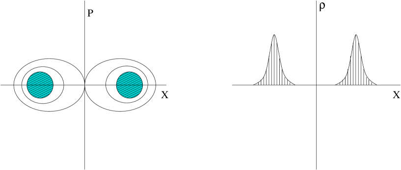
Figure 7: Density profile of the ‘analog’ fermions in the one-particle phase-space and in the eigenvalue space. The width of density profile is given by $\Delta\lambda\sim\left(\widetilde{e_{\rm F}}/\theta\right)^{1/2}$ and $\Delta p\sim\left(\widetilde{e_{\rm F}}\theta\right)^{1/2}$ so that $\Delta\lambda\Delta p\sim\widetilde{e_{\rm F}}$, consistent with Fermi statistics. In the classical limit, the profile reduces to delta-function distributions.

Classical Limit: $\hbar\rightarrow 0$

As a consistency check of the aforementioned three phases of the quantum NCFT, we will now examine the classical limit by taking $\hbar\to 0$, while holding $N$ large but fixed. First, from Eq.(4.11), we observe that the Planck constant $\hbar$ ought to be associated with $g^{2}_{\rm eff}$, as taking $g^{2}_{\rm eff}\equiv(N/{\rm}\theta)\rightarrow 0$ along with $N\rightarrow\infty$ renders the planar-phase to approach to the classical phase. In the notation of Eq.(4.11), this implies that the ‘t Hooft coupling scales as $g^{2}_{\rm eff}\sim N^{-\nu}\rightarrow 0$. Hence, in this subsection, we will take the Planck constant $\hbar$ equal synonymously to the ‘t Hooft coupling $g^{2}_{\rm eff}$.

Consider the double-well potential studied in the previous subsections. In the classical limit, we expect that profiles of the eigenvalue density field is reduced to those of classical phase, viz. vacua and solitons found in [3]. This can be understood as follows. For $E_{1},E_{2}$ below the potential barrier, each disconneced support of the eigenvalue density field $\rho_{\rm s}(\lambda)$ in Eq.(4.24) shrinks as $\hbar\sim g^{2}_{\rm eff}\rightarrow 0$, to a certain distribution of zero width, centered around $\lambda=\lambda_{1}$ and $\lambda=\lambda_{2}$, respectively. Examining the limit carefully, we find that

$$\frac{\rho_{\rm s}(\lambda)}{\hbar}\quad\longrightarrow\quad n_{1}\delta(\lambda-\lambda_{1})+n_{2}\delta(\lambda-\lambda_{2}),$$

reproducing accurately the classical profile of the eigenvalue density field, Eq.(4.6). Stated differently, starting from classical vacua and solitons Eq.(4.6) of Gopakumar, Minwalla and Strominger [3], turning on the quantum effects renders them into filled Fermi sea of the Hermitian matrix quantum mechanics, either on a single well or multiple wells. See fig 7.

To convince the readers that the classical limit is reproducible correctly, consider the simplest situation again – the single well potential $V(\lambda)=\frac{1}{2}\Omega^{2}\lambda^{2}$. Then, at large-$N$ limit, $E=N\hbar\Omega$ (ignoring the zero-point fluctuation energy), and Eq.(4.24) implies that

$$\int\limits_{-\infty}^{+\infty}{\rm d}\lambda\,\rho_{\rm s}(\lambda)\,=\,\frac{1}{N\hbar}\int\limits_{-\lambda_{0}}^{+\lambda_{0}}{\rm d}\lambda\sqrt{2\left(N\hbar\Omega-\frac{1}{2}\Omega^{2}\lambda^{2}\right)}=1$$

over the band $[-\lambda_{0},+\lambda_{0}]$. Here, we have used the following value of the turning point, defining the band-edge of the distribution:

$$\lambda_{0}=\sqrt{2N\hbar/\Omega}.$$

One immediately notes that Planck’s constant $\hbar$ is in the right place in Eq.(4.24), identifiable as $g^{2}_{\rm eff}\sim\hbar$. As $\hbar\rightarrow 0$, for a fixed but large $N$, the band-edge $\lambda_{0}$ scales to zero, and hence the band width shrinks to zero size. At the same time, the mid-band density scales as $\sqrt{\Omega/N\hbar}\rightarrow\infty$. Evidently, in the classical limit, product of the mid-band density times the band width remains constant and is always of order ${\cal O}(1)$.

As is well exploited in the context of matrix model description of $c=1$ noncritical string [18], profile of the density field $\rho(\lambda)$ is expressible alternatively using Wigner’s phase-space distribution function of the $N$ ‘analog’ fermions:

$${\rm F}(p,\lambda;t)\; = \,\int{\rm d}x\,\Psi^{\dagger}\left(\lambda-{\hbar\over 2}x,t\right)\,e^{{i\over\hbar}px}\,\Psi\left(\lambda+{\hbar\over 2}x,t\right)$$

$$= \,\int{\rm d}x\,\,\Psi^{\dagger}\left(\lambda,t\right)\,\star\,e^{{i\over\hbar}px}\star\Psi\left(\lambda,t\right).$$

Here, the coordinates $(\lambda,p)$ obey Moyal’s commutation relation, $[p,\lambda]_{\star}=i\hbar\,\,$. In terms of Wigner’s distribution function, the eigenvalue density field is expressed compactly as:

$$\rho(\lambda,t)={\hbar\over N}\int{\rm d}p\,{\rm F}(p,\lambda;t),$$

measuring the distribution of the eigenvalues. The factor of $\hbar$ reproduces correctly the normalization condition $\int{\rm d}p{\rm d}\lambda\,\hbar{\rm F}(p,\lambda;t)=1$. As shown in [32], the Wigner’s function corresponding to saddle-point configuration is simply given in the first-quantized description by the phase-space density of $N$ fermions. The fermions occupy the lowest $N$ energy eigenstates of the one-particle Hamiltonian ${\cal H}(\lambda)$ in Eq.(4.9).

4.7 Second-Quantized Description

Actually, using the second-quantized fermion field operators introduced in Eq.(4.19), the eigenvalue density field is now expressible as the fermion number density operator:

$$\hat{\rho}(\lambda,t)={1\over N}\Psi^{\dagger}(\lambda,t)\,\Psi\left(\lambda,t\right),$$ (4.26)

yielding correct normalization $\int{\rm d}\lambda\,\Psi^{\dagger}(\lambda,t)\Psi(\lambda,t)=N$. Taking expectation value of Eq.(4.26) on a many-particle state $|\lambda_{1},\ldots,\lambda_{N}\rangle$, antisymmetrized product of $N$ position eigenfunctions, we obtain

$$\left<\lambda_{1},\ldots,\lambda_{N}|\,\hat{\rho}(\lambda)\,|\lambda_{1},\ldots,\lambda_{N}\right>={1\over N}\sum_{\ell=1}^{N}\delta\Big{(}\lambda-\lambda_{\ell}(t)\Big{)},$$ (4.27)

matching perfectly with Eq.(4.5). It also satisfies the normalization condition

$$\int\limits_{-\infty}^{+\infty}{\rm d}\lambda\,\left<\,\hat{\rho}(\lambda,t)\,\right>=1.$$

The Eq.(4.27) implies that $\hat{\rho}(\lambda)$ operator is expressible as

$$\hat{\rho}(\lambda)={1\over N}\sum_{\ell=1}^{N}\delta\Big{(}\hat{\lambda}-\lambda_{\ell}(t)\Big{)},$$ (4.28)

where $\hat{\lambda}$ refers to the position operator in the first-quantized description. This then defines the density field operator at quantum level.

Equipped with the eigenvalue density field operator Eq.(4.28) via the second-quantized fermion field $\Psi$, one can exploit quantum effect to the NCFT vacua and solitons. Restricting low-energy excitations to the U$(\infty)$ invariant sector, we have found that classical dynamics of the tachyon field is described by the density field $\rho(\lambda)$. Likewise, in the same U$(\infty)$ invariant sector, quantum dynamics of the tachyon field is described by the density field operator $\hat{(}\hat{\lambda})$ defined in Eq.(4.28). The extent of quantum effects can be judged by taking expectation value of Eq.(4.28) and measuring deviation from its classical value Eq.(4.5). For instance, by approximating the eigenvalue density field operator to be the same as the classical distribution, we have obtained in the previous subsection that

$$\Big{<}\hat{\rho}(\lambda)\Big{>}=\frac{1}{\hbar}\sqrt{2(E-V(\lambda))}.$$

Equivalently, U$(\infty)$ invariant information of the tachyon field is governed by the change of variable:

$${1\over N}{\rm Tr}_{\cal H}{\bf T}^{n}=\int\limits_{-\infty}^{+\infty}{\rm d}\lambda\,\lambda^{n}\rho(\lambda).$$

Thus, from a knowledge of the classical $\rho(\lambda)$, one can reconstruct the classical tachyon field $\bf T$ in the Weyl formulation. One can subsequently rebuild the tachyon field ${\rm T}(x)$ on ${\hbox{\cmss R}\hbox to0.0pt{\hss\vrule height=8.0pt,width=0.8pt,depth=-0.1pt\hskip 0.6pt\phantom{.} }}^{2}$ via the Weyl-Moyal correspondence map. The reconstruction is equally applicable at quantum level. For instance,

$${1\over N}{\rm Tr}_{\cal H}\left<\widehat{\bf T}^{n}\right>=\int\limits_{-\infty}^{+\infty}{\rm d}\lambda\,\lambda^{n}\Big{<}\widehat{\rho}(\lambda)\Big{>}.$$

Denote the image of the Weyl-Moyal map of $\Big{<}\widehat{\bf T}\Big{>}$ as $\widehat{{\rm T}}({\bf x})$. Then, the above equation becomes

$${1\over V({\hbox{\cmss R}\hbox to0.0pt{\hss\vrule height=8.0pt,width=0.8pt,depth=-0.1pt\hskip 0.6pt\phantom{.} }}^{2}_{\theta})}\int_{{\hbox{\cmss R}\hbox to0.0pt{\hss\vrule height=8.0pt,width=0.8pt,depth=-0.1pt\hskip 0.6pt\phantom{.} }}^{2}_{\theta}}d^{2}{\bf x}\,\left[\widehat{{\rm T}}({\bf x})\star\widehat{{\rm T}}({\bf x})\star\cdots\star\widehat{{\rm T}}({\bf x})\right]_{\rm n-tuple}=\int\limits_{-\infty}^{+\infty}{\rm d}\lambda\lambda^{n}\Big{<}\widehat{\rho}(\lambda)\Big{>}.$$ (4.29)

This moment relation enables to reconstruct the ‘quantum’ profile of the vacua and solitons over ${\hbox{\cmss R}\hbox to0.0pt{\hss\vrule height=8.0pt,width=0.8pt,depth=-0.1pt\hskip 0.6pt\phantom{.} }}^{2}_{\theta}$ We will draw utility of the map by illustrating two representative physical consequences driven by the ‘quantum effects’.

         Quantum Destruction of Long-Range Order

We have already demonstrated that the quantum effect drives the classical density profile of delta-function type into a Fermi distribution, as depicted in Fig.(7). A consequence of broadening into the Fermi distribution is that the translational invariance over ${\hbox{\cmss R}\hbox to0.0pt{\hss\vrule height=8.0pt,width=0.8pt,depth=-0.1pt\hskip 0.6pt\phantom{.} }}_{\theta}^{2}$, viz. ${\bf x}^{a}\rightarrow{\bf x}^{a}+$ (constant), which is respected by all classical vacua, is dynamically broken.

Recall that the classical vacua correspond to density distribution of delta-function type, all eigenvalues taking the same value, say, ${\rm T}_{0}$. Thus, Eq.(4.29) yields

$${1\over V({\hbox{\cmss R}\hbox to0.0pt{\hss\vrule height=8.0pt,width=0.8pt,depth=-0.1pt\hskip 0.6pt\phantom{.} }}^{2}_{\theta})}\int_{{\hbox{\cmss R}\hbox to0.0pt{\hss\vrule height=8.0pt,width=0.8pt,depth=-0.1pt\hskip 0.6pt\phantom{.} }}^{2}_{\theta}}d^{2}{\bf x}\,\Big{(}\widehat{{\rm T}}({\bf x})\Big{)}^{n}_{\star}={\rm T}_{0}^{n}\qquad{\rm for}\qquad n=1,2,3,\cdots.$$

and hence find the unique solution as $\widehat{{\rm T}}({\bf x})={\rm T}_{0}$ — a homogeneous configuration, respecting the translational invariance over ${\hbox{\cmss R}\hbox to0.0pt{\hss\vrule height=8.0pt,width=0.8pt,depth=-0.1pt\hskip 0.6pt\phantom{.} }}^{2}_{\theta}$.

Once quantum effects are taken into account, as shown above, the classical delta-function type density distribution is broadened into a Fermi distribution putting each eigenvalue at a different value from one another – a consequence of repulsion between adjacent eigenvalues. In this case, it is fairly straightforward to convince oneself that there is no homogeneous solution solving the moment map Eq.(4.29) for all $n$. As such, a generic solution of Eq.(4.29) ought to be a nontrivial function over ${\hbox{\cmss R}\hbox to0.0pt{\hss\vrule height=8.0pt,width=0.8pt,depth=-0.1pt\hskip 0.6pt\phantom{.} }}^{2}_{\theta}$. To illustrate this, let us take

$$\Big{<}\widehat{\rho}(\lambda)\Big{>}=\left\{\begin{array}[]{ccc}1/R&{\rm for}&-R/2\leq\lambda\leq+R/2\\ 0&{\rm otherwise}&\\ \end{array}\right..$$ (4.32)

Then, a solution of Eq.(4.29) is easily found as

$$\widehat{{\rm T}}({\bf x})=\left\{\begin{array}[]{ccc}x^{1}&{\rm for}&-R/2\leq x^{1}\leq+R/2\\ 0&{\rm otherwise}&\end{array}\right.,$$ (4.35)

thus breaking translational invariance along the $x^{1}$-direction over ${\hbox{\cmss R}\hbox to0.0pt{\hss\vrule height=8.0pt,width=0.8pt,depth=-0.1pt\hskip 0.6pt\phantom{.} }}^{2}_{\theta}$, though invariant under translation along the $x^{2}$-direction. There are also infinitely many other solutions to Eq.(4.29), including the ‘stripe-phase’ states, but they are all related to the solution Eq.(4.35) via U($\infty$) rotations, viz. solutions of the type $U({\bf x})\star{\rm T}(x^{1})\star U^{-1}({\bf x})$ for an arbitrary ${\rm U}({\bf x})$.

We conclude that the translational long-range order of the classical vacua in NCFT is destroyed generically by quantum fluctuations.

         Quantum Corrected Soliton Mass

Consider the classical soliton of type $(N_{a},N_{b})$, Eq.(4.4). We are interested in estimating the mass of the ‘quantum’ soliton, or, equivalently, the quantum correction to the soliton mass. Take, for definiteness, the potential $V({\bf T})$ of the type given in Fig.(3). Classically, the soliton mass is simply given by the increase of the potential energy by moving, out of total $N=N_{L}+N_{L}$ eigenvalues situated at the global vacuum on the left well, a fraction of $N_{R}$ eigenvalues to the local minima on the right well. Denoting the energy difference between the left and the right wells, $V_{L},V_{R}$, as $\Delta V=(V_{R}-V_{L})$, the classical soliton mass is given by

$$M_{(N_{L},N_{R})}[{\rm classical}]\quad\sim\quad\theta N_{R}\Delta V.$$

Quantum mechanically, eigenvalue distribution for both the global vacuum and the $(N_{L},N_{R})$ soliton will be broadened into Fermi distributions. Thus, the quantum corrected soliton mass is estimated by computing the difference of the energy functional averaged over the Fermi distributions according to Eq.(4.29). Utilizing the results of Eqs.(4.12, 4.13), we estimate the quantum corrected soliton mass as

$$M_{(N_{L},N_{R})}[{\rm quantum}] = \Big{<}{\cal E}_{(N_{L},N_{R})}\Big{>}-\Big{<}{\cal E}_{(N_{L}+N_{R},0)}\Big{>}$$

$$\sim \left({\rm}\theta N_{L}V_{L}+N_{L}^{2}\right)+\left({\rm}\theta N_{R}V_{R}+N_{R}^{2}\right)-\left({\rm}\theta NV_{L}+N^{2}\right)$$

$$= M[{\rm classical}]-2N_{L}N_{R}.$$

We thus deduce that the quantum correction, as given by the second term in the last expression, is negative and is of order ${\cal O}(N^{2})$. Evidently, the correction is negligible in the GMS-phase, comparable in the planar-phase, but outweighs the classical mass in the disordered phase.

5 Discussions

Before closing, we would like to bring up investigation of related phenomena in other contexts. The first is concerning quantum effects either in IKKT Type IIB or in BFSS Type IIA matrix theories. For Type IIB IKKT matrix model, the issue of measure-induced interaction between eigenvalues and its consequences have been considered previously, albeit in different context and with different motivation. See, for instance, results of [33] and references therein. The classical moduli space is given by ten commuting matrices whose eigenvalues span ${\hbox{\cmss R}\hbox to0.0pt{\hss\vrule height=8.0pt,width=0.8pt,depth=-0.1pt\hskip 0.6pt\phantom{.} }}^{10}$, ten-dimensional Euclidean spacetime. A calculation of the matrix partition function indicates that the moduli space is partly lifted and, morally speaking, a smaller-dimensional submanifold remains nocompact and flat. The result is attributed to a logarithmic interaction between eigenvalues as the remaining “angular” degrees of freedom are integrated out. This is similar to the vandermonde effect of the one-matrix model.

Classical solutions of the IKKT and BFSS matrix models include all of the D-branes in Type IIA and IIB strings. The low-energy theory is equivalent to NCFTs involving both scalar and gauge fields. An immediate question is whether there exist various kinds of large-$N$ limits in these field theories, some of which might destabilize the D-branes by quantum fluctuations. We believe that this is a very important issue, so let us remark a little further. One place to look for this sort of effect would be one-loop computations in the IKKT and BFSS matrix models which might show the necessity of a sort of ’tHooft-like scaling, viz. $\theta\sim N$, without which the D-brane solutions might be completely destabilized, which is the counterpart of the disordered phase studied in this paper. Of course, for D$p$ branes or a system of D$p$-D$q$ branes (with $p=q$ mod 4) bosonic and fermionic determinants cancel because of supersymmetry and there are no large-$N$ divergences at 1-loop. On the other hand, supersymmetry is broken in situations involving (i) relative motion between the BPS branes, (ii) D$p$-D$q$ branes with $p-q$ not a multiple of 4, and (iii) brane-antibrane systems. In (iii), the $D2-\bar{D}2$ system [34, 35] was studied extensively, and it would be an interesting starting place to address the large-$N$ issues raised here.

Second, as elaborated in section 2.7, the measure effect we have discussed in this paper is intimately related to the phenomenon of IR divergence [21] through nonplanar diagrams. Recently, it has been shown [36] that the completion of all the nonplanar diagrams participating in the UV-IR mixing in NCFTs studied in this work is expressible entirely in terms of scalar counterpart of the open Wilson lines [37]. The effective action then interpreted as (Legendre transform of) an effective field theory of noncommutative dipoles – noncommutative manifestation of dynamically generated ‘closed strings’ [38]. There, the result was based exclusively on the Moyal formulation. An interesting problem is to recast the result in Weyl formulation, and to understand the three different scaling regimes in terms of the open Wilson lines and noncommutative dipoles.

Finally, it would be interesting to see if the transition to the disordered phase discussed in this paper is related to the large $N$ phase transition [26].

We will report progress regarding the above problems elsewhere.

Acknowledgement

We are grateful to S.R. Das, A. Dhar, M.R. Doulgas, R. Gopakumar, D.J. Gross, V. Kazakov, S. Minwalla, S. Mukhi, A. Sen, and S.H. Shenker for enlightening discussions. We would like to thank hospitality of Theory Division at CERN (GM and SJR), Institut Henri Poincaré (SJR), and Institut des Hautes Ètudes Scientifiques (SJR) during this work.

Appendix A Weyl-Moyal correspondence

In this section we briefly review the operator formulation of NCFT in the context of Sec 2.1.

One begins by introduce an ‘auxiliary’ one-particle Hilbert space ${\cal H}$, of dimension ${\tt dim}{\cal H}=N$, carrying a representation of the Heisenberg algebra:

$$\left[\widehat{x^{a}},\widehat{x^{b}}\right]=i\epsilon^{ab}{\hbox to0.0pt{\rm I\hss}\hskip 2.6pt\hbox{\rm I}}.$$

The Weyl-Moyal map refers to isomorphism between functions on ${\hbox{\cmss R}\hbox to0.0pt{\hss\vrule height=8.0pt,width=0.8pt,depth=-0.1pt\hskip 0.6pt\phantom{.} }}^{2}_{\theta}$ and operators on ${\cal H}$:

$${\bf x}\quad \longleftrightarrow \quad\widehat{\bf x}$$

$${\rm T}({\bf x})\quad \longleftrightarrow \quad{\bf T}(\widehat{{\bf x}})$$

$$V_{\star}(T)\quad \longleftrightarrow \quad V({\bf T})$$

$$\int{\rm d}^{2}{\bf x}\cdots\,\, \longleftrightarrow \quad{{\rm Tr}}_{{\cal H}_{\theta}}\cdots,.$$ (A.1)

In particular, in plane-wave basis, the Weyl-Moyal map renders the following one-to-one correspondence between fields:

$${\rm T}({\bf x})=\int_{\widetilde{\hskip 5.69046pt{\hbox{\cmss R}\hbox to0.0pt{\hss\vrule height=8.0pt,width=0.8pt,depth=-0.1pt\hskip 0.6pt\phantom{.} }}^{2}}}{{\rm d}^{2}{\bf k}\over(2\pi)^{2}}\,e^{-i{\bf k}\cdot{\bf x}}\,{\rm Tr}_{{\cal H}}\left(e^{i{\bf k}\cdot\widehat{\bf x}}\,{\bf T}\right),$$ (A.2)

which follows from Weyl-ordering prescription of the operators $\widehat{\bf x}$’s.

The map, Eq.(A.1), then equates the NCFT action Eq.(2.4) with Eq.(2.6). Operators on ${\cal H}$ are realizable in terms of matrices once we introduce a complete set of orthonormal basis of ${\cal H}$ as $|\ell\rangle$, $\ell=1,2,\cdots,{\tt dim}{\cal H}\equiv N$, and one-dimensional projection operators therein:

$${\bf P}_{\ell}\,\,=\,\,|\ell\rangle\langle\ell|\qquad\qquad\ell=1,2,\cdots,{\tt dim}{\cal H}\equiv N.$$ (A.3)

The ${\bf P}_{\ell}$’s satisfy the projective and the completeness relations:

$${\bf P}_{\ell}{\bf P}_{m}\,\,=\,\,\delta_{\ell m}{\bf P}_{m}\qquad\quad{\rm and}\quad\qquad\sum_{\ell=1}^{N}{\bf P}_{\ell}={\hbox to0.0pt{\rm I\hss}\hskip 2.6pt\hbox{\rm I}}.$$

At leading order in $(1/{\rm}\theta)$, both Eq.(2.4) and (2.6) are invariant under

$${\rm T}({\bf x})\rightarrow U({\bf x})\star{\rm T}({\bf x})\star U^{-1}({\bf x})\qquad\longleftrightarrow\qquad{\bf T}\rightarrow{\bf U}{\bf T}{\bf U}^{-1},$$ (A.4)

representing area-preserving diffeomorphism, equivalently, U$(\infty)$ symmetry. The symmetry is broken explicitly by the term ${\cal L}_{-1}$.

Appendix B Large $N$ Saddle-Point of One-Matrix Model

As mentioned in Sec 2.4, taking $\theta=N/g^{2}_{\rm eff}$ and small enough $g_{\rm eff}$, we have seen that the large-$N$ saddle-point for the density $\rho_{s}$ ($\rho$ defined in Eq.(2.7)) is simply an extremum of the effective action Eq.(2.22) (with the constraint Eq.(2.21) taken care of by a lagrange multiplier $E$):

$$S_{\rm total}[\rho]=S_{\rm eff}[\rho]+E\Big{(}1-\int_{\cal D}{\rm d}\lambda\rho(\lambda)\Big{)}.$$ (B.1)

The saddle-point equation for $\rho$ then reads:

$$\partial_{\rho}S_{\rm total}[\rho]=N^{2}\left[g^{-2}_{\rm eff}V(\lambda)-2\int_{\cal D}{\rm d}\mu\rho(\mu)\ln|\lambda-\mu|\right]-N\theta E=0\qquad{\rm for}\quad\lambda\subset{\cal D},$$ (B.2)

viz. analytically continuing to complex-$\lambda$ plane, the real-part of

$$V_{\rm eff}(\lambda)=V(\lambda)-2g^{2}_{\rm eff}\int_{\cal D}{\rm d}\mu\,\rho(\mu)\ln(\lambda-\mu)$$

remains constant $E$ over the support ${\cal D}$. Taking derivative of Eq.(B.2) with respect to $\lambda$, one obtains the following dispersion-relation:

$${1\over 2g^{2}_{\rm eff}}V^{\prime}(\lambda)=\int_{\cal D}\hskip-14.22636pt-\hskip 11.38092pt{\rm d}\mu\,{\rho(\mu)\over\lambda-\mu}\qquad{\rm for}\quad\lambda\subset{\cal D}.$$

The right-hand side is related to the resolvent ${\cal R}(\lambda)$ of the eigenvalue distribution:

$${\cal R}(\lambda):=\lim_{N\rightarrow\infty}\left<{1\over N}{\rm Tr}{1\over\lambda-{\bf T}}\right>=\int_{\cal D}{\rm d}\mu\,{\rho(\mu)\over(\lambda-\mu)},\qquad{\rm Re}{\cal R}(\lambda)=\int_{\cal D}\hskip-14.22636pt-\hskip 11.38092pt{\rm d}\mu\,{\rho(\mu)\over(\lambda-\mu)},$$ (B.3)

supplemented with the boundary condition

$${\cal R}(\lambda)={1\over\lambda}+{\cal O}\left({1\over\lambda^{2}}\right)\qquad{\rm for}\qquad\lambda\rightarrow\infty$$

as the consequence of the normalization condition

$$\int{\rm d}\lambda\,\rho(\lambda)=1.$$

Consider now the potential Eq.(2.8). Let us look for a saddle-point corresponding to the $(N_{1},N_{2})$-instantons. Evidently, extending the above results, quantum counterpart of $(N_{1},N_{2})$ instantons ought to correspond to so-called two-cut distributions in matrix model. The two-cut distribution is characterized by two disjoint intervals ${\cal D}_{1},{\cal D}_{2}$ and fractions of eigenvalue density:

$$n_{1}=\int_{{\cal D}_{1}}{\rm d}\lambda\,\rho(\lambda)\quad{\rm and}\quad n_{2}=\int_{{\cal D}_{2}}{\rm d}\lambda\,\rho(\lambda)\qquad{\rm with}\quad n_{1}+n_{2}=1.$$

At large-$N$, large-$\theta$ limit, the total action is now given by

$$S_{\rm total}[\rho;n_{1},n_{2}]=S_{\rm eff}[\rho]+E_{1}\left(n_{1}-\int_{{\cal D}_{1}}{\rm d}\lambda\,\rho(\lambda)\right)+E_{2}\left(n_{2}-\int_{{\cal D}_{2}}{\rm d}\lambda\,\rho(\lambda)\right).$$

The saddle-point equation for $\rho(\lambda)$ takes the same form as before, viz.:

$$N^{2}\left(g^{-2}_{\rm eff}V(\lambda)-2\int_{{\cal D}_{1}}{\rm d}\mu\rho(\mu)\ln|\lambda-\mu|\right) = N\theta E_{1}\qquad\quad{\rm for}\qquad\lambda\subset{\cal D}_{1}$$

$$N^{2}\left(g^{-2}_{\rm eff}V(\lambda)-2\int_{{\cal D}_{2}}{\rm d}\mu\rho(\mu)\ln|\lambda-\mu|\right) = N\theta E_{2}\qquad\quad{\rm for}\qquad\lambda\subset{\cal D}_{2}.$$

The saddle-point equation with respect to $n_{1}$ yields:

$$\partial_{n_{1}}S_{\rm total}[\rho;n_{1},n_{2}]=\Big{(}E_{1}-E_{2}\Big{)}=0.$$ (B.4)

For the double-well potential of the type Eq.(2.8), the distribution on the two wells is symmetric. Using the methods mentioned above (see [15, 24] for more details), one finds that the saddle-point is given in terms of two-cut eigenvalue distribution Eq.(2.32).

References

- [1] A. Connes, M. R. Douglas and A. Schwarz, JHEP 9802, 003 (1998) [hep-th/9711162]/
- [2] N. Seiberg and E. Witten, JHEP 9909, 032 (1999) [hep-th/9908142].
- [3] R. Gopakumar, S. Minwalla and A. Strominger, JHEP 0005, 020 (2000) [hep-th/0003160].
- [4] M. Aganagic, R. Gopakumar, S. Minwalla and A. Strominger, JHEP 0104, 001 (2001) [hep-th/0009142].
- [5] L. Hadasz, U. Lindstrom, M. Rocek and R. von Unge, JHEP 0106, 040 (2001) [hep-th/0104017].
- [6] R. Gopakumar, M. Headrick and M. Spradlin, [hep-th/0103256].
- [7] N. Nekrasov and A. Schwarz, Commun. Math. Phys. 198, 689 (1998) [hep-th/9802068].
- [8] D. J. Gross and N. A. Nekrasov, JHEP 0007, 034 (2000) [hep-th/0005204].
- [9] A. P. Polychronakos, Phys. Lett. B 495, 407 (2000) [hep-th/0007043].
- [10] D. P. Jatkar, G. Mandal and S. R. Wadia, JHEP 0009, 018 (2000) [hep-th/0007078].
- [11] K. Dasgupta, S. Mukhi and G. Rajesh, JHEP 0006, 022 (2000) [hep-th/0005006].
- [12] E. Witten, [hep-th/0006071].
- [13] J. A. Harvey, P. Kraus, F. Larsen and E. J. Martinec, JHEP 0007, 042 (2000) [hep-th/0005031].
- [14] G. Mandal and S.-J. Rey, Phys. Lett. B 495, 193 (2000) [hep-th/0008214].
- [15] E. Brezin, C. Itzykson, G. Parisi and J. B. Zuber, Commun. Math. Phys. 59, 35 (1978).
-
[16]
E. . Brezin and S. R. Wadia,
The Large N expansion in quantum field theory and statistical
physics: From spin systems to two-dimensional gravity (World Scientific,
Singapore, Singapore, 1993);
M.L. Mehta, Random matrices, 2nd ed. (Academic Press, New York, 1991);
P.A. Mello, Theory of random matrices, Les Houches Session LXI, eds. E. Akkermans, G. Montambaux, J.L. Pichard, J. Zinn-Justin (North-Holland Pub. Co., Amsterdam, 1994). -
[17]
M. R. Douglas and S. H. Shenker,
Nucl. Phys. B 335, 635 (1990);
D. J. Gross and A. A. Migdal, Phys. Rev. Lett. 64, 127 (1990);
D. J. Gross and A. A. Migdal, Phys. Rev. Lett. 64, 717 (1990);
M. R. Douglas, Phys. Lett. B 238, 176 (1990). -
[18]
D. J. Gross and N. Miljkovic,
Phys. Lett. B 238, 217 (1990);
E. Brezin, V. A. Kazakov and A. B. Zamolodchikov, Nucl. Phys. B 338, 673 (1990);
P. Ginsparg and J. Zinn-Justin, Phys. Lett. B 240, 333 (1990);
G. Parisi, Phys. Lett. B 238, 209 (1990). - [19] N. Ishibashi, H. Kawai, Y. Kitazawa and A. Tsuchiya, Nucl. Phys. B 498, 467 (1997) [hep-th/9612115].
- [20] T. Banks, W. Fischler, S. H. Shenker and L. Susskind, Phys. Rev. D 55, 5112 (1997) [hep-th/9610043].
- [21] S. Minwalla, M. Van Raamsdonk and N. Seiberg, JHEP 0002, 020 (2000) [hep-th/9912072].
- [22] S.-J. Rey, talk given at ”Strings 2001”-International Conference at Tata Institute for Fundamental Research (Mumbai, India) http://theory.theory.tifr.res.in/strings/Proceedings/#rey-t.
-
[23]
A. Sen,
JHEP 9808, 012 (1998)
[hep-th/9805170];
A. Sen, JHEP 9912, 027 (1999) [hep-th/9911116];
A. Sen and B. Zwiebach, JHEP 0003, 002 (2000) [hep-th/9912249]. - [24] G. Bhanot, G. Mandal and O. Narayan, Phys. Lett. B 251, 388 (1990).
- [25] M. Van Raamsdonk, [hep-th/0110093].
-
[26]
D. J. Gross and E. Witten,
Phys. Rev. D 21 (1980) 446;
S. Wadia, EFI-79/44-Chicago preprint (KEK Scanned Version);
S. R. Wadia, Phys. Lett. B 93, 403 (1980). - [27] R.P. Feynman, Statistical Mechanics (Benjamin Pub. Co., Boston, 1972).
- [28] B. Sakita, Quantum Theory of Many-Variable Systems and Fields (World Scientific Pub. Co., Singapore, 1985).
- [29] M. Creutz, Rev. Mod. Phys. 50, 561 (1978).
-
[30]
A. Jevicki and B. Sakita,
Nucl. Phys. B 165, 511 (1980);
S. R. Das and A. Jevicki, Mod. Phys. Lett. A 5, 1639 (1990);
A. M. Sengupta and S. R. Wadia, Int. J. Mod. Phys. A 6, 1961 (1991);
D. J. Gross and I. R. Klebanov, Nucl. Phys. B 352, 671 (1991). - [31] D. J. Gross and I. Klebanov, Nucl. Phys. B 344, 475 (1990).
-
[32]
A. Dhar, G. Mandal and S. R. Wadia,
Mod. Phys. Lett. A 7, 3129 (1992)
[hep-th/9207011];
ibid. Mod. Phys. Lett. A 8, 3557 (1993) [hep-th/9309028]. - [33] J. Ambjorn, K. N. Anagnostopoulos, W. Bietenholz, F. Hofheinz and J. Nishimura, [hep-th/0104260].
-
[34]
O. Aharony and M. Berkooz,
Nucl. Phys. B 491, 184 (1997)
[hep-th/9611215];
G. Lifschytz and S. Mathur, Nucl. Phys. B 507, 621 (1997) [hep-th/9612087]. -
[35]
G. Mandal and S.R. Wadia,
Nucl. Phys. B 599, 137 (2001)
[hep-th/0011094];
P. Kraus, A. Rajaraman and S.H. Shenker, . Nucl. Phys. B 598, 169 (2001) [hep-th/0010016]. -
[36]
Y. Kiem, S.-J. Rey, H.-T. Sato and J.-T. Yee,
[hep-th/0106121];
Y. Kiem, S.-J. Rey, H.-T. Sato and J.-T. Yee, [hep-th/0107106];
Y. Kiem, S.-S. Kim, S.-J. Rey and H.-T. Sato, [hep-th/0110066];
Y. Kiem, S. Lee, S.-J. Rey and H.-T. Sato, [hep-th/0110215]. -
[37]
N. Ishibashi, S. Iso, H. Kawai and Y. Kitazawa,
Nucl. Phys. B 573, 573 (2000)
[hep-th/9910004];
S.-J. Rey and R. von Unge, Phys. Lett. B 499, 215 (2001) [hep-th/0007089];
S. R. Das and S.-J. Rey, Nucl. Phys. B 590, 453 (2000) [hep-th/0008042];
D. J. Gross, A. Hashimoto and N. Itzhaki, [hep-th/0008075];
A. Dhar and S. R. Wadia, Phys. Lett. B 495, 413 (2000) [hep-th/0008144]. - [38] S.-J. Rey, Exact Answers to Approximate Questions: Noncommutative Dipole, Open Wilson Line, and UV-IR Duality, Proceedings of ‘New Ideas in String Theory’, APCTP-KIAS Workshop (June, 2001) and of ‘Gravity, Gauge Theories, and Strings’, Les Houches Summer School (August, 2001), to appear.