Relativistic Stars in Randall-Sundrum Gravity

Abstract

The non-linear behavior of Randall-Sundrum gravity with one brane is examined. Due to the non-compact extra dimension, the perturbation spectrum has no mass gap, and the long wavelength effective theory is only understood perturbatively. The full 5-dimensional Einstein equations are solved numerically for static, spherically symmetric matter localized on the brane, yielding regular geometries in the bulk with axial symmetry. An elliptic relaxation method is used, allowing both the brane and asymptotic radiation boundary conditions to be simultaneously imposed. The same data that specifies stars in 4-dimensional gravity, uniquely constructs a 5-dimensional solution. The algorithm performs best for small stars (radius less than the AdS length) yielding highly non-linear solutions, core photons being redshifted by up to ${\cal Z}\simeq 12$. An upper mass limit is observed for these small stars, and the geometry shows no global pathologies. The geometric perturbation is shown to remain localized near the brane at high densities, the confinement interestingly increasing for both small and large stars as the upper mass limit is approached. Furthermore, the static spatial sections are found to be approximately conformal to those of AdS. We show that the intrinsic geometry of large stars, with radius several times the AdS length, is described by 4-dimensional General Relativity far past the perturbative regime, the largest stars being tested up to a core redshift of ${\cal Z}\simeq 2.1$. This indicates that the non-linear long wavelength effective action remains local, even though the perturbation spectrum has no mass gap. The implication is that Randall-Sundrum gravity, with localized brane matter, reproduces relativistic astrophysical solutions, such as neutron stars and massive black holes, consistent with observation.

1 Introduction

Branes with matter confined upon them have now become an essential component of string theory. Required by quantum theory on the world-sheet, they have tremendous classical implications in the low energy effective theory. New classes of compactifications are possible where the matter is localized to the brane itself, unlike Kaluza-Klein style compactifications where matter resides on the whole internal space. The weakness of gravity then makes probing such dimensions extremely difficult experimentally, leading to the idea that they may be very large compared to Standard Model energy scales [1, 2]. A simple ‘compactification’ of this type is a model with just one non-compact extra dimension, Randall-Sundrum gravity [3, 4]. With one asymptotically flat brane, no moduli problem, and only a negative cosmological constant in the bulk, it provides a very clean testing ground for gravitational studies. Intended as a toy model, work has shown it is possible to embed this theory into higher dimensional super-gravities [5, 6].

Linear and second order perturbation studies of one brane Randall-Sundrum [7, 8, 9, 10] show that for localized objects much larger than the AdS length, a brane observer views a local effective behavior which is simply 4-dimensional gravity. In Kaluza-Klein type compactifications, only the homogeneous modes play a significant role for long wavelength perturbations. However, the non-linear behavior of models with localized matter is a less tractable problem as the solutions can not be homogeneous. Matter sources on the brane inevitably generate inhomogeneity in the transverse space. Indeed, linear theory shows that in one brane Randall-Sundrum, the inhomogeneous eigenmodes in the transverse coordinate play a crucial role in ensuring a regular horizon geometry. With no mass gap in the perturbative spectrum, non-linearity induced by brane matter is not yet understood analytically. In particular, it is not clear how far into the non-linear regime the effective 4-dimensional description, shown to hold in the linear theory, remains valid.

The aim of this paper is to investigate the 5-dimensional non-linear geometry of static stars in one brane Randall-Sundrum gravity. Stars that are both small and large with respect to the AdS length are studied. We study the geometry of small stars, where curvatures due to the presence of matter are as large as the AdS curvature scale. We expect that the qualitative behavior of these dense objects will be similar in the one brane Randall-Sundrum model to other orbifold models. For large stars, we examine whether a local effective description remains in the non-linear regime. Our key results are;

• We find an elliptic method to solve the full non-linear, 5-dimensional, axi-symmetric Einstein equations. This elliptic approach enables us to simultaneously solve both the brane matching conditions and also the asymptotic AdS condition, ensuring regular, well defined horizon geometries. The same data for 4-dimensional star solutions uniquely generates a regular bulk geometry.

• The upper mass limit for stars of fixed radius is reproduced, both for small and large radii. The brane is unable to stabilize ultra dense stars.

• The effective description for long wavelength perturbations, corresponding to astrophysical objects, remains that of 4-dimensional gravity far into the non-linear regime.

• The perturbation of the geometry from AdS remains localized for non-linear stars of all radii, the decay of the perturbation steepening near the upper mass limit.

• The spatial sections of both small and large stars are found to be approximately conformal to those of AdS.

This paper only studies the non-compact case of Randall-Sundrum gravity. We later see that the ease of imposing boundary conditions in one brane Randall-Sundrum makes this an attractive model to test. For compact models the method could also be applied, with the boundary conditions suitably altered, and is left for future investigation.

We organize the paper as follows. In the remainder of the first section we briefly review the non-linear behavior of 4-dimensional stars and then Kaluza-Klein and Randall-Sundrum gravities. We discuss why non-linearity is not well understood in localized matter compactifications. In the second section we highlight the main results of the paper, in order to put the following methods and calculations in context.

The third section discusses the method used to pose the bulk 5-dimensional Einstein equations in a framework suitable for elliptic solution numerically. The regular metric is chosen to have a residual conformal symmetry and results in elliptic second order derivatives of the unknown metric functions in a sufficient subset of the Einstein equations. Furthermore, it enables the brane to be fixed at constant coordinate position whilst the asymptotic horizon metric takes a simple form. This conformal symmetry allows the structure of the constraint equations to be compatible with the elliptic relaxation, implying that all the Einstein equations are satisfied even though only a subset are relaxed. The method is tested and found to work well for configurations where the star radius is up to a few times the AdS length. This is already a large enough scale to see the 4-dimensional effective behavior emerge. As a consistency check, in the fourth section, the 5-dimensional linear theory is also computed numerically by an independent method and excellent agreement is found in the low density regime.

The fifth section outlines the solutions obtained. The scheme is able to generate fully non-linear regular solutions. Strong evidence for an upper mass limit is found by observing stars smaller than the AdS length. For these the numerical method is most stable and allows highly non-linear solutions to be calculated that trace the critical behavior very close to this limit. Geodesics are constructed to probe the global features of the static spatial geometry, which is found to contain no pathologies, and interestingly is approximately conformal to the spatial sections of AdS. For the larger stars, those that are well described by 4-dimensional effective theory in the linear regime, we again calculate non-linear configurations. We are able to calculate solutions which are fully non-linear, where brane observables deviate from the linear prediction by several times, and cannot therefore be described in higher order perturbation theory. The confinement of the geometric perturbation to the brane is found to increase near the upper mass limit for both small and large stars. The large star solutions are seen to very closely follow the 4-dimensional effective gravity description for all levels of non-linearity tested, despite this increase in confinement with stellar density. This strongly suggests that the correct description of long range behavior in Randall-Sundrum gravity is simply 4-dimensional gravity, even in the non-linear regime, provided the effective 4-dimensional curvature scale remains below that set by the bulk cosmological constant, as for neutron stars and large black holes away from the singularity. In order to observe significant deviations from 4-dimensional physics one would then need to observe short wavelength perturbations or possibly dynamical effects over long time scales [11].

1.1 Stars in 4-dimensions

The behavior of static spherical matter in the non-linear regime of general relativity is quite different from that in the Newtonian limit. We briefly review the relevant features. Consider a star composed of perfect fluid so that,

$$T_{\mu\nu}=\rho\,u_{\mu}u_{\nu}+P\left(g_{\mu\nu}+u_{\mu}u_{\nu}\right)$$ (1)

with $u_{\mu}u^{\mu}=-1$. Assuming a static spherically symmetric metric, one must specify the density profile, and together with metric regularity and the requirement of asymptotically flat space, the Einstein equations, $G_{\mu\nu}=8\pi GT_{\mu\nu}$, can be integrated. An analytic solution exists for the simple top-hat density profile,

$$\rho(r)=\begin{cases}\rho_{0}&(r\leq R)\\ 0&(r>R)\end{cases}$$ (2)

where one finds a static regular solution with ADM mass $M=m(\infty)=\frac{4}{3}\pi R^{3}\rho_{0}$ provided the density is below a critical value. Specifically the maximum attainable mass solution is

$$M_{\rm max}=\frac{4}{9}\,8\pi R$$ (3)

when units of $8\pi G=1$ are chosen, and therefore, for a given $R$ there is an upper bound to the mass of a static star, the core pressure becoming infinite as $M\rightarrow M_{\rm max}$. Note that this is a purely non-linear effect. In the Newtonian theory there is no upper mass limit for this equation of state, the core pressure simply scaling quadratically with $\rho_{0}$. The core pressure characterizes this critical behavior, with $P_{\rm c}<<\rho_{0}$ for Newtonian stars, $P_{\rm c}\sim\rho_{0}$ being the regime where the onset of non-linearity occurs and $P_{\rm c}\rightarrow\infty$ for critical mass stars. Note that in these isotropic coordinates $R$ is the proper angular radius of the star, giving the size of the $S^{2}$ associated with the spherical symmetry, at the edge of the star. When we subsequently refer to a radius, we shall mean the proper angular radius. It is interesting to note that for a general, physically reasonable equation of state, $M_{\rm max}\leq\frac{4}{9}\,8\pi R$ for fixed $R$ [12]. Thus uniform density, (2), is the equation of state giving the largest critical mass for a given radius. It is for this reason that we use a (slightly smoothed) top-hat as the density profile in the 5-dimensional solutions we construct later.

Observations indicate neutron stars are extremely relativistic objects with $M\sim M_{\odot}$ and $R\sim 1{\rm km}$ so that $GM/R\sim 1$ [12]. Taking a uniform density equation of state with $\rho_{0}$ to be a typical nuclear density and ignoring rotation, this provides an upper mass limit of $\sim 5M_{\odot}$ for neutron stars [13]. If this result were considerably less then stellar collapse would generically yield black holes and the population of neutron stars of this radius would be zero. Conversely if the result were much larger then collapse to a black hole may be difficult for the majority of stellar objects.

1.2 Randall-Sundrum Gravity

Now we review 5-dimensional Randall-Sundrum gravity with a single $Z_{2}$ orbifold brane [3]. Whilst being a simple and elegant theory that reproduces 4-dimensional linear gravity for long wavelength perturbations, it has the crucial advantage that there are no moduli fields to be stabilized as occurs generically for compact extra dimensions. Unless otherwise stated, when referring to Randall-Sundrum, it is implicit that we mean the one brane case, with the brane being asymptotically flat.

The bulk matter is merely a negative cosmological constant and the brane tension and matter localized on the brane are treated in a distributional sense [14]. Varying the action,

$$S=\frac{1}{L^{3}}\int d^{5}x\sqrt{-g}\left(\frac{R}{2}-\Lambda\right)+\frac{1}{L^{3}}\int_{\rm{brane}}d^{4}y\sqrt{-h}\left(\sigma+{\cal L}_{\rm{brane}}\right)$$ (4)

where the localized stress energy tensor $T_{\mu\nu}/L^{3}$ is derived as,

$$-\frac{1}{2}T_{\mu\nu}=\frac{\partial{\cal L}_{\rm{brane}}[h_{\mu\nu}]}{\partial h_{\mu\nu}}$$ (5)

giving the bulk Einstein equations,

$$G^{(5)}_{\mu\nu}=-\Lambda g_{\mu\nu}$$ (6)

and Israel thin shell matching conditions implementing the orbifold $Z_{2}$ symmetry,

$$2\left[K_{\mu\nu}-h_{\mu\nu}K\right]_{\rm{brane}}=\left(-\sigma h_{\mu\nu}+T_{\mu\nu}\right)$$ (7)

with $L$ the 5-dimensional Planck length, $\Lambda/L^{3}$ the bulk cosmological constant, $K_{\mu\nu}$ the projection of the extrinsic curvature of the brane hyper-surface with induced metric $h_{\mu\nu}$ and tension $\sigma/L^{3}$. Note the appropriate Gibbons-Hawking boundary term is suppressed above.

The tension of the brane, $\sigma/L^{3}$, is chosen to admit static solutions where the bulk metric is AdS and can be written as,

$$ds^{2}=\frac{l^{2}}{z^{2}}\left(ds^{2}_{(\rm 4-Mink)}+dz^{2}\right)$$ (8)

where $ds^{2}_{(\rm 4-Mink)}$ is 4-dimensional Minkowski space, $l$ is the AdS radius and is given by $\Lambda=-6/l^{2}$. More generally, when the bulk is perturbed by matter, $l$ still gives the curvature length associated with the cosmological constant, and is related to the Ricci scalar as $l^{2}=-20/{\cal R}$. Localized matter on the brane is taken to be of perfect fluid form, as in equation (1), so the physical density is $\rho/L^{3}$. The hyper-surface $z=0$ is the conformal boundary of AdS, and $z\rightarrow\infty$ the horizon. A vacuum brane (vanishing $T_{\mu\nu}$), intrinsically flat and with tension $\sigma/L^{3}$, where, $\sigma=6/l$, can be located on the hyper-surface $z=z_{0}$.

Note that we can always choose $z=l$ by rescaling the coordinates as $z\rightarrow\frac{l}{z_{0}}z$ together with $x_{\mu}\rightarrow\frac{l}{z_{0}}x_{\mu}$ which is a natural scale invariance of this AdS metric. Indeed we shall use a metric whose form is invariant under conformal transformations in the $r,z$ plane, that allows the brane to be placed at fixed $z$ independent of the matter on it, whilst asymptotically towards the horizon the metric can still tend to the simple form of (8). Throughout the following sections we choose units based on the AdS length, and therefore $l=1$, implying that $-\Lambda=\sigma=6$ and the brane location is $z=1$.

We may use a homogeneous ansatz, analogous to the Kaluza-Klein one, namely,

$$ds^{2}=\frac{l^{2}}{z^{2}}\left(g_{\mu\nu}(x^{\alpha})dx^{\mu}dx^{\nu}+dz^{2}\right)$$ (9)

where the perturbation is homogeneous in $z$, only depending on $x^{\mu}$, up to scaling by the warp factor. This does solve the bulk Einstein equations provided $g_{\mu\nu}(x^{\alpha})$ is 4-dimensionally Ricci flat [15], as for example in the black string solution [16, 17, 18]. Note that there is no physical dilaton $\phi$ as now $z$ is not an angular coordinate [19]. Indeed, this ansatz is the non-linear extension of the linearized zero mode as is the case for the Kaluza-Klein ansatz [20]. However, the ansatz above only applies to vacuum brane configurations. Furthermore, consider regularity for this geometry at large $z$. The 5-dimensional Weyl components, $C_{\mu\nu}^{~{}~{}\alpha\beta}$, with indices as they would appear in curvature invariants, are related to the 4-dimensional ones of the metric $g_{\mu\nu}(x^{\alpha})$ by a factor of $(z/l)^{2}$ and thus diverge, along with curvature invariants, at large $z$. Without a fundamental theory it remains unclear whether such singularities are pathological [16, 20].

We will only be concerned with geometries that have a regular horizon and thus are dynamically well defined. Therefore, when matter sources are present on the brane, boundary conditions must be imposed on the geometry asymptotically far from the brane. More precisely we consider the radiation boundary conditions of [7]. Then for static solutions, the scalar propagator in AdS decays towards the horizon. The linear response of the brane geometry to matter localized on it is found to be 4-dimensional standard General Relativity at long distances compared to the AdS length $l$, [8, 7]. The relation between the 5-dimensional Planck scale and the 4-dimensional one, $G=G_{5}/l$ allows a range of $l$ from $\sim 1{\rm mm}$ (the limit of gravity measurement [2, 21, 22]), corresponding to a 5-dimensional Planck length, $L\sim(10^{8}{\rm GeV})^{-1}$, to the more conventional scheme where $l$ and $L$ are both 4-dimensional Planck length valued. The scale $l$ allows us to define the terms large and small for static objects in the 4-dimensional induced theory on the brane. Low density linear astrophysical objects reside in the large regime, and are indistinguishable in the 4-dimensional and 5-dimensional theory. Small objects are distinguished already at the linear level and may have relevance at early times in the universe [23].

One way to characterize the induced geometry is to use the Gauss-Codacci geometric decomposition [24, 25], where the unknown bulk geometry is parameterized in the projection of the bulk Weyl tensor onto the brane. Some analytic progress has been made in the vacuum case. An elegant solution for a black hole was obtained for a 3-dimensional brane in a 4-dimensional bulk [26]. No generalization to 5-dimensions has so far been found. The solution is not of the black string type [16] having a regular horizon. General restrictions on the horizon in 5-dimensions were considered in [27], and making some assumptions, the type of asymptotic geometry was characterized using a ‘no hair’ argument in [28]. Cosmological solutions [29, 30, 31, 32] show that a 4-dimensional effective description is recovered at late times. Integrable cosmological solutions [33] can be analytically continued to give exact localized domain wall solutions [34, 35]. These remarkably agree exactly with a 4-dimensional effective gravity description. The AdS-CFT conjecture allows one to write the form of the corrections to effective 4-dimensional gravity as a contribution from a CFT on the induced geometry with a mass cut-off [7, 36, 37, 38, 39, 40, 28].

Two attempts have been made numerically to solve the bulk geometry non-linearly. Time symmetric initial data was constructed for a black hole spacetime indicating that the localization to the brane is recovered non-linearly in this initial data [41]. Whether such localization survives dynamically remains an open and difficult question. An attempt has also been made to solve the static black hole geometry numerically by a hyperbolic evolution into the bulk, making an ansatz for initial data on the brane [42]. This again indicates localization non-linearly with pancake like horizons, but generically the metric evolves into singular configurations not far from the brane. This is a problem of a hyperbolic approach, integrating the metric away from the brane, where one must know exactly what initial data to take on the brane in order to ensure that asymptotically the metric tends to AdS. A recent work [43] studied relativistic stars by making an ansatz for the bulk Weyl tensor projection. Whilst some progress is possible, allowing one to consider the intrinsic corrections to the effective theory from terms quadratic in the stress tensor of the localized matter, one has no reason to assume the form of the Weyl projection. Furthermore, one has no control over the bulk and horizon geometry, and the configurations studied are most likely pathological away from the brane. As Randall-Sundrum gravity is only well defined when the horizon boundary conditions are specified, we concentrate here on solving for the full bulk geometry including both the asymptotic properties and the brane boundary conditions. We only expect a well defined, regular 5-dimensional geometry when the radiation boundary conditions are imposed as in the linear theory.

2 Highlights of Results

We now highlight the main results obtained in the paper. The details involved in the calculations can be found later, in particular the numerical scheme that allows the full non-linear calculation of the bulk geometry. However we wish to present the main results to give the context in which the rather technical calculations were performed.

• Upper Mass Limit for Small Stars - Figure 1
  The numerical method we outline performs most stably for small stars, with radius less than the AdS length. Extremely non-linear solutions can be found in this case. Figure 1 shows the ratio of core pressure to density for a (smoothed) top-hat density profile with fixed coordinate radius $\xi=0.3$ (see equation (31)) yielding solutions with proper radius $R\sim 0.3$. Newtonian theory predicts a linear dependence of $P/\rho$ on $\rho$. We clearly see a departure from this behavior and strong evidence that the core pressure diverges for finite core density, $\rho\simeq 7$. The numerical method does not give a convergent solution if a larger core density is used. Note that for small stars the behavior is not that of 4-dimensional GR. However the qualitative nature of the upper mass limit for fixed radius appears to persist to small stars. For large stars we cannot approach this limit so closely, but the indications are that again an upper mass limit would be found as the behavior follows 4-dimensional GR so closely (see below). A detailed description of this result is found in section 5.1.

• Non-Linear Long Range Effective Theory - Figure 2
  In order to calculate the 5-dimensional geometries for stars, we input a density profile and require isotropy on the brane. The matching conditions impose these requirements as boundary conditions. Once the solution is found we may read off the corresponding pressure profile on the brane. The redshift of photons propagating in the brane from the core of the star to some radius can be computed. The core pressure and the core redshift of a photon emitted to infinite distance on the brane are both coordinate scalar quantities for this static spherical symmetry. Given the density profile against proper distance for the 5-dimensional solution one can compute exactly the same quantities in standard 4-dimensional gravity. A comparison then allows one to assess how good an effective description the 4-dimensional theory is. Figure 2 shows both the core redshift and pressure for Randall-Sundrum stars with various radii. The 5-dimensional value is plotted against the same quantity calculated in the 4-dimensional theory for the same density profile. We see that for increasing $\xi$, which is approximately equal to the proper radius of the star, the difference between the 4-dimensional and 5-dimensional values decrease. Already for $\xi=3$, only three times the AdS length, the predictions differ by only $\sim 20\%$. Note that a curve is also drawn to show how the linear approximation compares to full non-linear 4-dimensional GR for the $\xi=3$ case. This shows that the solutions found clearly probe the fully non-linear regime, where one cannot meaningfully apply higher order perturbation theory. The level of agreement depends on the proper size of the object, $R\simeq\xi$, as expected. The crucial result is that it does not appear to depend on the core density. Perturbation theory predicts agreement for small density, but we see full non-linear agreement. The implication in then that the full non-linear 4-dimensional effective theory is standard GR. Furthermore, by observing neutron star physics or massive black hole horizon geometries accessible through astrophysical measurements, we will be unable to differentiate between Randall-Sundrum and 4-dimensional gravity. A detailed description of this result is found in section 5.4.

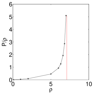
Figure 1: An illustration of core pressure, $P$, against core density, $\rho$, for configurations with $\xi=0.3$ (see equation for density profile (31)). The proper angular radii vary monotonically from $R=0.30\,-\,0.38$ from low to high density. The behavior strongly indicates a diverging core pressure for finite density, implying that for small stars an upper mass limit for a given $R$ exists. The brane does not act to stabilize the large densities. The curve appears qualitatively similar to the usual 4-dimensional incompressible fluid star behavior. (all lattices: $dr=0.02$, $r_{\rm max}=2$, $dz=0.005$, $z_{\rm max}=4$. systematic errors from comparison with linear theory in section 4 are estimated at $\sim 2\%$)

  

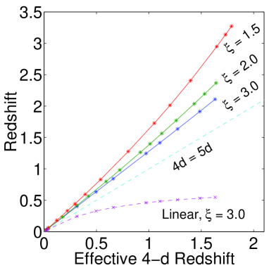
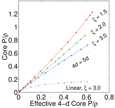
Figure 2: An illustration of 4-d against 5-d behavior; On the left the actual core redshift of a star, calculated from the 5-dimensional geometry, is plotted as a function of the same quantity calculated from the induced 4-dimensional effective theory. On the right, the core pressure divided by density is plotted in the same way. Three values of, $\xi=1.5,2,3$ are used to generate solutions for different core densities $\rho$. $\xi$ approximately corresponds to the proper radius, $R$, of the star. One clearly sees that the larger the star, the closer the solutions lie to the ‘4d = 5d’ $45^{o}$ line. In the data presented moving vertically down towards this line the proper radius of the star increases. Furthermore, for each $\xi$, the points fall approximately on straight lines. This indicates that the goodness of approximation of 5-dimensional theory by the effective 4-dimensional one is roughly independent of the core density, and hence non-linearity, over the range tested. The degree of approximation depends only on the star size. The most non-linear $\xi=3$ stars are at $\sim 75\%$ of their upper mass limit in the 4-dimensional effective theory. The last line plotted is the 4-dimensional linear theory prediction for the $\xi=3$ stars, again against the 4-dimensional non-linear theory. We see that the linear theory deviates strongly from this, showing that the solutions probed are fully non-linear, and beyond the reach of higher order perturbation theory. These graphs are strong evidence that the effective 4-dimensional description applies far into the non-linear regime, and probably right up to the upper mass limit. (lattices: $\xi=1.5$: $dr=0.10$, $r_{\rm max}=10$, $dz=0.02$ and $0.04$, $z_{\rm max}=21$, $\xi=2.0$: $dr=0.15$, $r_{\rm max}=15$, $dz=0.02$ and $0.04$, $z_{\rm max}=31$, $\xi=3.0$: $dr=0.20$, $r_{\rm max}=20$, $dz=0.03$ and $0.05$, $z_{\rm max}=46$. two lattice $dz$ resolutions are used to extrapolate to $dz=0$. systematic errors from comparison with linear theory in section 4 are estimated to be maximum for $\xi=3.0$ at $\sim 10\%$.)

3 Solving By Elliptic Relaxation

Our task is to construct solutions to Randall-Sundrum gravity sourced by static spherically symmetric matter distributions on the 4-dimensional brane, such as those corresponding to stars. In order to do this one must solve the full non-linear Einstein equations with boundary conditions given by the matter localized on the brane and that the asymptotic geometry is that of AdS as in the linear theory with radiation boundary conditions.

A static spherical star in the induced brane geometry requires that the metric in the bulk has an axial symmetry. This now becomes a problem in two variables, with a radial, $r$, and an axial, $z$, coordinate. In the linear theory [8, 7] one can choose a synchronous gauge with respect to the background $z$ coordinate in (8) allowing the metric perturbation components to decouple. There is no such decoupling in the non-linear theory, and thus one expects to have to solve a system of coupled non-linear partial differential equations.

Figure 3 schematically illustrates the boundary data for the problem. The brane matching conditions are non-linear equations relating normal derivatives of metric functions to the functions themselves. Asymptotically we wish to recover AdS, again placing constraints on the metric functions. We return to the nature of these boundary conditions later but it is sufficient now to note that conditions are specified on the brane and asymptotic boundaries of the $r,z$ space. This is not data defined on a Cauchy surface as in an ADM evolution, but rather is elliptic data.

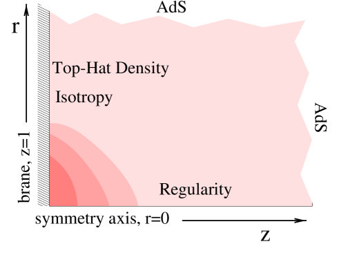
Figure 3: An illustration of the asymptotic and brane boundary data.

One can always perform an ADM decomposition in the $z$ direction and solve the bulk metric from initial data given on the brane, as in [42]. However, we see from figure 3 that one has to supply initial data on the brane that ensures asymptotically AdS behavior far from the brane. In the linear theory one can construct the Greens function only from modes obeying this condition. In the full theory one has no such luxury, and indeed it was found in [42] that data on the brane generically evolves to give pathologies far from the brane. If one then wishes to solve this 2 variable problem using a ‘hyperbolic’ evolution from one boundary, such as the brane, or from large $z$ inwards, then one is confronted with a shooting problem as the data is naturally defined on all the boundaries. Furthermore this is a shooting problem in 2 variables and therefore one is shooting with functions rather than constants as in familiar 1 variable shooting problems. Therefore the framework we will use to solve the bulk equations is not that of a hyperbolic evolution, but rather by an elliptic relaxation. A simple example where gravity can be solved elliptically is in static 4-dimensional linear theory, which in a Newtonian gauge results in a Poisson equation for the potential. One more generally expects static GR to result in an elliptic problem. In 4-dimensions the vacuum axi-symmetric problem reduces to solving a Laplace equation [44], although this does not generalize to higher dimension [45]. In this paper we show that in 5-dimensions, the system can indeed be solved elliptically for this symmetry.

3.1 Relaxation for a brane star in Randall-Sundrum gravity

The problem now is to identify a coordinate system where the equations might admit a solution via a relaxation method with elliptic boundary conditions. We know of no general method to find such a choice for static solutions in gravity. Instead we sketch a brief argument for why the gauge we have chosen is suitable.

We wish to describe regular static geometries with axial symmetry (induced spherical symmetry on the brane). We therefore consider a manifold, topologically equivalent to that of the static vacuum Randall-Sundrum solution and take the metric,

$$ds^{2}_{5}=\frac{1}{z^{2}}\left[-e^{2T(r,z)}dt^{2}+e^{2R(r,z)}dr^{2}+e^{2S(r,z)}r^{2}d\Omega_{2}^{2}+e^{2Z(r,z)}dz^{2}+2e^{2v(r,z)}drdz\right]$$ (10)

which is the most general parameterization of such a geometry. We still have 2 degrees of coordinate freedom in $r$ and $z$ which we shall use to eliminate 2 metric functions and obtain a gauge suitable for relaxation.

We wish to obtain bulk Einstein equations for the 3 remaining metric functions that have elliptic differential operators in the second derivative terms for $r,z$. Firstly we note that the off diagonal term generically gives rise to hyperbolic second derivative terms in Einstein equations of the form $v_{,rz}$ and therefore we eliminate this with the residual coordinate freedom. For this diagonal metric, $R$ is a lapse function with respect to the $r$ direction and therefore no equation will contain $R_{,rr}$ derivatives. Similarly, $Z$ is a lapse function with respect to $z$ and there are no $Z_{,zz}$ derivatives entering the equations. This can be seen if one substitutes the diagonal metric into the Einstein bulk action, and linearizes, giving, to lowest order in terms that give rise to second derivatives in the Einstein equations,

$${\cal S}^{\rm{2^{{\rm nd}}\,Deriv}}\simeq \int drdz\frac{r^{2}}{z^{3}}\left(2\,\partial_{z}R\,\partial_{z}S+{({\partial_{z}S})^{2}}+\partial_{z}R\,\partial_{z}T+2\,\partial_{z}S\,\partial_{z}T\right.$$

$$\qquad\qquad\left.+{({\partial_{r}S})^{2}}+2\,\partial_{r}S\,\partial_{r}T+2\,\partial_{r}S\,\partial_{r}Z+\partial_{r}T\,\partial_{r}Z\right)$$ (11)

The full non-linear action can be varied and reproduces 4 of the 5 Einstein field equations, the $G^{r}_{~{}z}$ equation being missing, but implied from the others by the Bianchi identities. The $R$ and $Z$ equations will, as mentioned, not contain second order elliptic operators due to their lapse nature.

If the gauge choice $R=Z$ is also imposed using the remaining coordinate degree of freedom then this linearized Lagrangian becomes symmetric in these second derivative terms,

$${\cal S}^{\rm{2^{{\rm nd}}\,Deriv}}_{R=Z}\simeq \int drdz\frac{r^{2}}{z^{3}}\left(2\,\partial_{z}R\,\partial_{z}S+{({\partial_{z}S})^{2}}+\partial_{z}R\,\partial_{z}T+2\,\partial_{z}S\,\partial_{z}T\right.$$

$$\qquad\qquad\left.+2\,\partial_{r}R\,\partial_{r}S+{({\partial_{r}S})^{2}}+\partial_{r}R\,\partial_{r}T+2\,\partial_{r}S\,\partial_{r}T\right)$$

$$= \int drdz\frac{r^{2}}{z^{3}}\left(M_{ij}(\partial_{r}V^{(i)})(\partial_{r}V^{(j)})+\left[\partial_{r}\leftrightarrow\partial_{z}\right]\right)$$ (12)

to lowest order, were the vector $V=\left\{T,R,S\right\}$. Now the $T,R,S$ equations contain second derivative terms which are symmetric in $r$ and $z$ and thus are individually elliptic Laplace operators. The matrix $M_{ij}$ has one positive and two negative eigenvalues indicating that the system is not positive definite. Therefore we cannot guarantee $T,R,S$ will relax simultaneously, but individually (ignoring singularities from $r,z=0$ terms) the equations for $T,R,S$ are elliptic to linear order and hence we can attempt to relax them together. Note that we are only considering a subset of the Einstein equations as varying the action yields the Einstein equations associated with the Einstein tensor components $G^{t}_{~{}t},G^{\theta}_{~{}\theta}$ and $G^{r}_{~{}r}+G^{z}_{~{}z}$, which we term the ‘elliptic’ Einstein equation components. We later consider how the remaining equations, $G^{r}_{~{}z}$ and $G^{r}_{~{}r}-G^{z}_{~{}z}$, are consistent with elliptic relaxation. We term these equations ‘constraints’, as they are implied from the other Einstein equation components by the two non-trivial Bianchi identity components. Note that they do contain second order derivatives, although they are not elliptic. We use the term constraint as, in section 3.3, we see the Bianchi identities imply that they must be satisfied in the interior of the problem if they are satisfied on the boundaries and the elliptic equations $G^{t}_{~{}t}=6,G^{\theta}_{~{}\theta}=6$ and $G^{r}_{~{}r}+G^{z}_{~{}z}=12$ are satisfied in the interior. This is therefore analogous to the case of hyperbolic evolution, where provided the constraints are satisfied on a Cauchy surface, they will remain satisfied upon integration of the evolution equations.

For future convenience we set,

$$R =A+B$$

$$S =A-B$$ (13)

and the metric is now,

$$ds^{2}_{5}=\frac{1}{z^{2}}\left[-e^{2T(r,z)}dt^{2}+e^{2\left(A(r,z)+B(r,z)\right)}\left(dr^{2}+dz^{2}\right)+e^{2\left(A(r,z)-B(r,z)\right)}r^{2}d\Omega_{2}^{2}\right]$$ (14)

and yields the full non-linear equations,

$$\nabla^{2}T= \left[-2\,(\partial_{r}A)\,(\partial_{r}T)+2\,(\partial_{r}B)\,(\partial_{r}T)-{({\partial_{r}T})^{2}}\right]+\left[\,\partial_{r}\leftrightarrow\partial_{z}\,\right]$$

$$-\frac{2}{r}\,{\partial_{r}T}+\frac{1}{z}\left({2\,\partial_{z}A}-{2\,\partial_{z}B}+{4\,\partial_{z}T}\right)+{\frac{4}{{z^{2}}}}\,\left(e^{2\,(A+\,B)}-1\right)$$

$$\nabla^{2}A= \left[-\frac{1}{2}(\partial_{r}A)^{2}+(\partial_{r}A)\,(\partial_{r}B)-\frac{1}{2}(\partial_{r}B)^{2}+\frac{1}{2}(\partial_{r}A)\,(\partial_{r}T)-\frac{1}{2}(\partial_{r}B)\,(\partial_{r}T)\right]+\left[\,\partial_{r}\leftrightarrow\partial_{z}\,\right]$$

$$+\frac{1}{r}\left(-\partial_{r}A+\partial_{r}B+\frac{1}{2}\partial_{r}T\right)+\frac{1}{z}\left(\frac{1}{2}\partial_{z}A-\frac{1}{2}\partial_{z}B-\frac{1}{2}\partial_{z}T\right)+\frac{1}{z^{2}}\,\left(e^{2\,(A+\,B)}-1\right)$$

$$\nabla^{2}B= \left[\frac{3}{2}\,(\partial_{r}A)^{2}-3\,(\partial_{r}A)\,(\partial_{r}B)+\frac{3}{2}\,(\partial_{r}B)^{2}+\frac{3}{2}\,(\partial_{r}A)\,(\partial_{r}T)-\frac{3}{2}\,(\partial_{r}B)\,(\partial_{r}T)\right]+\left[\,\partial_{r}\leftrightarrow\partial_{z}\,\right]$$

$$+\frac{1}{r}\left(3\,\partial_{r}A-3\,\partial_{r}B+\frac{3}{2}\,\partial_{r}T\right)+\frac{1}{z}\left(-\frac{9}{2}\,\partial_{z}A+\frac{9}{2}\,\partial_{z}B-\frac{3}{2}\,\partial_{z}T\right)$$

$$-\frac{1}{r^{2}}\left(e^{4\,B}-1\right)-\frac{3}{z^{2}}\left(e^{2\,\left(A+B\right)}-1\right)$$ (15)

with $\nabla^{2}=\partial_{r}^{2}+\partial_{z}^{2}$. These equations for $T,A,B$ are linear combinations of the elliptic Einstein equations, denoted $\{tt\},\{rr+zz\},\{\theta\theta\}$ after removing a homogeneous $z^{2}$ blue-shifting factor for convenience, as described in appendix 8.1. These must be supplemented with the remaining Einstein equations, $G^{r}_{~{}z}=0$ and $G^{r}_{~{}r}-G^{z}_{~{}z}=0$, the constraints, similarly rescaled and denoted $\{rz\}$ and $\{rr-zz\}$,

$$\{rz\}=\partial_{r}\partial_{z} \left(2B-2A-T\right)+\frac{4}{r}\,\partial_{z}B+\frac{1}{z}\left(-3\,\partial_{r}A-3\,\partial_{r}B\right)$$

$$+2\,(\partial_{r}A)\,(\partial_{z}A)+2\,(\partial_{z}A)\,(\partial_{r}B)+2\,(\partial_{r}A)\,(\partial_{z}B)-6\,(\partial_{r}B)\,(\partial_{z}B)$$

$$+(\partial_{z}A)\,(\partial_{r}T)+(\partial_{z}B)\,(\partial_{r}T)+(\partial_{r}A)\,(\partial_{z}T)+(\partial_{r}B)\,(\partial_{z}T)-(\partial_{r}T)\,(\partial_{z}T)=0$$ (16)

and $\{rr-zz\}$,

$$\{rr-zz\}= \left[-2\partial^{2}_{r}A+2\partial^{2}_{r}A-2\partial^{2}_{r}T\right]-\left[\partial_{r}\leftrightarrow\partial_{z}\right]$$

$$+\frac{8}{r}\partial_{r}B+2(\partial_{r}A)^{2}+4(\partial_{r}A)(\partial_{r}B)-6(\partial_{r}B)^{2}+2(\partial_{r}A)(\partial_{r}T)+2(\partial_{r}B)(\partial_{r}T)-(\partial_{r}T)^{2}$$

$$+\frac{6}{z}\left(\partial_{z}A+\partial_{z}B\right)-2(\partial_{z}A)^{2}-4(\partial_{z}A)(\partial_{z}B)+6(\partial_{z}B)^{2}-2(\partial_{z}A)(\partial_{z}T)$$

$$-2(\partial_{z}B)(\partial_{z}T)+(\partial_{z}T)^{2}=0$$ (17)

The metric functions $T,A,B$ enter these two constraint equations $\{rz\}$ and $\{rr-zz\}$ with hyperbolic second derivatives $\partial_{r}\partial_{z}$ and $\partial_{r}^{2}-\partial_{z}^{2}$ respectively. For reference the Einstein tensor components are given in appendix 8.1.

It is important at this point to raise the issue that one might be able to solve for remaining metric functions algebraically or by integration of a constraint, and therefore have to relax fewer metric functions in the $r,z$ plane. We have no reason to suggest that such a scheme could not be used but were unable to find such a scheme that used the constraints directly. Integrating a function over the lattice using the hyperbolic nature of the constraints is extremely non-local compared to one iteration of a local Poisson equation solver such as Gauss-Seidel. This non-locality was generically found not to yield convergent schemes. In fact, $R=A+B$ can be thought of as a lapse function, and can actually be algebraically determined directly from the $\{rr+zz\}$ Einstein equation, the corresponding Hamiltonian constraint. This could be used directly to eliminate this metric function, but again the remaining variables could not be relaxed. The only scheme we found to work was one where the 3 metric functions were all elliptically relaxed together.

Each bulk equation, (15), appears to contain second order elliptic operators, but there are singular terms as $r\rightarrow 0$. It is certainly true is that away from $r=0$ the second order operators are non-singular and therefore can individually be solved by elliptic relaxation. However, whilst each equation individually appears elliptic, when avoiding singular points, the three taken together are not necessarily so. Experimentally we do fortunately find that for a straightforward numerical scheme the three can indeed be consistently relaxed together. The scheme to deal with the singular terms is discussed in detail in the later section 3.6.

The following sections consider the boundary data for the relaxation. We examine,

• the boundary data that must be specified on the brane and asymptotically.

• how the constraint equations are satisfied through the boundary data when only the elliptic bulk equations are relaxed.

• how to specify data at the origin where singular terms are present.

3.2 Local Conformal Symmetry and Brane Coordinate Position

With the gauge choice discussed in the previous section, the metric (14) still has residual coordinate freedom, namely 2-dimensional conformal transformations, $\bar{r}=f(r,z),\bar{z}=g(r,z)$,

$$d\bar{r}^{2}+d\bar{z}^{2}=\Omega(r,z)\left(dr^{2}+dz^{2}\right)$$ (18)

so that $f,g$ satisfy the usual Cauchy-Riemann relations. The data for such a transformation can be taken as specifying $g$ on all boundaries and $f$ at one point on any boundary. This always allows the brane to be moved by such a transformation from $\bar{z}_{\rm brane}=1$ to $z_{\rm brane}=1+h(r)$ where $h$ is an arbitrary function. For example, we could take $g(r,1)=1+h(r)$, $g(r=\infty,z)=z+h(r=\infty)$, and $g(r,z\rightarrow\infty)=z+h(r=\infty)$, and in addition, $\partial_{r}g=0$ at $r=0$ implying $f(r=0,z)=0$, taking $f(r=0,z=\infty)=0$.

Note that a crucial feature of this transformation is that provided $h(r)$ decays to zero as $r$ increases, the metric is asymptotically unaffected by such a transformation. The solution to the Laplace equation for $g$ with the data above is then $g=z$ plus a perturbation from $h(r)$ that dies away as $\frac{1}{z}$ far away from the brane, and so $g\rightarrow z,f\rightarrow r$ as $z\rightarrow\infty$. For example, consider the static vacuum Randall-Sundrum metric in variables $\bar{r},\bar{z}$ after such a conformal transformation to $r,z$, which yields,

$$ds^{2}_{5}=\frac{1}{z^{2}}\left[\left(\frac{z}{g}\right)^{2}\left(-dt^{2}+\left(g_{,r}^{2}+g_{,z}^{2}\right)\left(dr^{2}+dz^{2}\right)+\left(\frac{f}{r}\right)^{2}r^{2}d\Omega_{2}^{2}\right)\right]$$ (19)

As $f\rightarrow r,g\rightarrow z$ and the derivatives $g_{r}\rightarrow 0$, $g_{z}\rightarrow 1$ for large $r$ or large $z$, asymptotically the metric will tend to the static Randall-Sundrum solution, (8). Thus, local transformations of the coordinate position of the brane only effect the metric locally. We are able to consistently position the brane at $z=1$ and again the asymptotic behavior is that $T,A,B\rightarrow 0$ as $r$ or $z\rightarrow\infty$. This is shown explicitly in appendix 8.2 for the linear theory.

The significance of this is considerable. Contrast this for instance with the synchronous gauge used in the linearized analyses [7, 8] where the residual gauge transformations $\xi_{5}=\xi_{5}(x)$, and $\xi_{\mu}=\xi_{\mu}(x)$, can be used to move the brane coordinate position. A relaxation scheme in this gauge would either have to remain in the ‘Randall-Sundrum’ transverse gauge, where the horizon metric remains simple, and include a new degree of freedom in the relaxation which would represent the position of the brane, or alternatively place the brane at a fixed coordinate location, using a Gaussian normal gauge, which perturbs the metric asymptotically and therefore requires a complicated and non-local boundary condition asymptotically that would encode this degree of freedom. Then the metric would no longer decay to the simple form of (8). Either case is complicated and with no guarantee of convergent relaxation, may be unlikely to work.

In summary, the conformal gauge was chosen to yield equations (15) that have elliptic second order operators allowing relaxation methods to be applied. Conveniently we see it also allows the brane to be consistently placed at fixed coordinate location, say $z=1$, and the asymptotic behavior is simply $T,A,B\rightarrow 0$ as $r$ or $z\rightarrow\infty$ for radiation boundary conditions.

3.3 Brane Boundary Data

In order to solve the system we must specify the matter on the brane by satisfying the brane matching conditions (38) of appendix 8.1. In addition, we will also show that only one of the two constraint equations must be enforced on the brane itself. It will be shown in the subsequent section 3.5 that the condition $T,A,B\rightarrow 0$ as $r,z\rightarrow\infty$ is sufficient to ensure the constraints are then satisfied everywhere.

In 4-dimensional gravity, static spherical symmetry requires two metric functions to parameterize the geometry. Two conditions are required to fix these degrees of freedom in the solution. One can take these to be specifying a density profile, and requiring isotropy, so that $G^{r}_{~{}r}=G^{\theta}_{~{}\theta}=P(r)$ thus fixing the radial and angular pressure component to be equal. Together with asymptotic boundary conditions in $r$, the metric can be solved for.

On the brane in the 5-dimensional case we have the same two conditions, a density profile and isotropy. However we now have 3 metric functions $T,A,B$. Using the matching conditions (38) these become

$$\rho=-\sigma-2\,\left(-3+3\,z\,\partial_{z}A-z\,\partial_{z}B\right)\,e^{-(A+B)}$$ (20)

and for isotropy the simpler linear condition,

$$B_{,z}=0$$ (21)

This fixes two metric components, say $A$ and $B$, leaving the remaining component $T$. There are also additional constraint equations. Since all the matter dependent data will be specified on the brane, the asymptotic boundary data being simply that the metric tend to AdS at the horizon, these constraints must fix $T$ in order to have agreement between the physical data of 4-dimensional and Randall-Sundrum gravity.

Calculating the non-trivial components of the Bianchi identities $\nabla_{\mu}G^{\mu}_{~{}\nu}=0$ for the metric (14), and assuming that the elliptic Einstein equations, $\{tt\},\{rr+zz\},\{\theta\theta\}$ are satisfied, yields,

$$\frac{1}{g}\,\left[\,\partial_{r}\left(g\,G^{r}_{~{}z}\right)+\partial_{z}\left(\frac{g}{2}\,\left(G^{r}_{~{}r}-G^{z}_{~{}z}\right)\right)\,\right] =0$$

$$\frac{1}{g}\,\left[\,\partial_{z}\left(g\,G^{r}_{~{}z}\right)-\partial_{r}\left(\frac{g}{2}\,\left(G^{r}_{~{}r}-G^{z}_{~{}z}\right)\right)\,\right] =0$$ (22)

where $g=\sqrt{-\det{g_{\mu\nu}}}$. Thus the quantities $g\,G^{r}_{~{}z}$ and $g\left(G^{r}_{~{}r}-G^{z}_{~{}z}\right)$ satisfy Cauchy-Riemann relations and therefore separately satisfy Laplace equations. An example of data for the system is to specify $g\,G^{r}_{~{}z}$ on all boundaries, and $g\left(G^{r}_{~{}r}-G^{z}_{~{}z}\right)$ at only one point.

Thus if $G^{r}_{~{}z}=0$ is used to determine $T$ on the brane, and $g\,G^{r}_{~{}z}$ is also zero asymptotically away from the brane then provided $g\left(G^{r}_{~{}r}-G^{z}_{~{}z}\right)$ vanishes at one point, say asymptotically, the pair of constraints will also be solved everywhere, provided the elliptic Einstein equations are satisfied in the bulk. The vanishing of these quantities asymptotically is discussed in the later section 3.5. Note also that as $g\,G^{r}_{~{}z}$ satisfies a Laplace equation, this zero data on all boundaries has the unique solution that $\{rz\}$ and $\{rr-zz\}$ are true everywhere within.

On the brane we choose to use $\{rz\}$ to determine $T$. One can see from equation (16) that this constraint has a linear second order differential operator acting on $T$ which is hyperbolic with characteristics in the $r$ and $z$ directions, so that it can be integrated in from $r=\infty$ to $r=0$ along the brane. Now all 3 of the metric functions are determined on the brane by the constraints, density and isotropy conditions and the 5-dimensional brane data is consistent with that of the 4-dimensional system. Thus we expect, and indeed find that the same stellar data as for standard 4-dimensional GR uniquely specifies the 5-dimensional bulk geometry.

3.4 Linearized Equations and Their Solution Numerically

We now construct the solution to the linear theory in the conformal gauge described above. As there is no matter in the bulk except for the cosmological constant, using the synchronous transverse traceless gauge for the linear perturbations one finds that the perturbing metric components decouple and can be solved using a Greens function. Such solutions are given in [7, 8]. In this section we explicitly coordinate transform back to a metric of the form (14) for a spherical static brane source. One must now only solve decoupled equations with simple boundary conditions, and this is used to provide an independent check of the full non-linear method in section 4.

Firstly perturb the static Randall-Sundrum metric, (8) as follows,

$$ds^{2} =\frac{1}{\bar{z}^{2}}\left(ds^{2}_{\rm(pert)}+d\bar{z}^{2}\right)$$

$$ds^{2}_{\rm(pert)} =-\left(1-6a-2\bar{r}\partial_{\bar{r}}a\right)dt^{2}+\left(1+2a\right)d\bar{r}^{2}+\bar{r}^{2}\left(1+2a+\bar{r}\partial_{\bar{r}}a\right)d\Omega_{\rm 2}^{2}$$ (23)

where $a=a(\bar{r},\bar{z})$, which is the synchronous transverse traceless gauge. The linearized constraint equations $\{rz\},\{rr-zz\}$ are satisfied and the 3 bulk equations reduce to,

$$\nabla^{2}_{\rm{(AdS)}}a=\left(\partial_{\bar{r}}\partial_{\bar{r}}+\partial_{\bar{z}}\partial_{\bar{z}}+\frac{4}{\bar{r}}\,\partial_{\bar{r}}-\frac{3}{\bar{z}}\,\partial_{\bar{z}}\right)a=0$$ (24)

an elliptic operator acting on $a$. As discussed in [7, 8] the transverse traceless condition does not allow coordinate freedom to place the brane at $\bar{z}=1$.

The coordinate transformation to bring the metric into the form (14) is then $\bar{r}=r+f(r,z)$, $\bar{z}=z+g(r,z)$ with,

$$\partial_{r}g =-\partial_{z}f$$

$$\partial_{z}g =\partial_{r}f+a$$ (25)

which yield Poisson equations for $f,g$,

$$\nabla^{2}f =-\partial_{r}a$$

$$\nabla^{2}g =\partial_{z}a$$ (26)

where $\nabla^{2}=\partial^{2}_{r}+\partial^{2}_{z}$. Equation (24) for $a$ is unchanged to linear order as $\bar{r},\bar{z}\rightarrow r,z$. The coordinate transformed metric components $T,A,B$ are then,

$$T =-3\,a-r\,\partial_{r}a-{\frac{g}{z}}$$

$$A =a+\frac{1}{2}\,\partial_{r}f+{\frac{f}{2r}}+\frac{r}{4}\,\partial_{r}a-{\frac{g}{z}}$$

$$B =\frac{1}{2}\,\partial_{r}f-{\frac{\,f}{2r}}-\frac{r}{4}\,\partial_{r}a$$ (27)

in terms of $a,f,g$, and now the boundary conditions on the brane can be calculated from the brane matching conditions, equations (38) in appendix 8.1, if one places the brane at $z=1$ in the ‘conformal metric’ coordinates, giving,

$$\nabla^{2}_{\rm{(3-d)}}g =\partial^{2}_{r}g+\frac{2}{r}\partial_{r}g=\frac{1}{6\,z}\rho$$

$$\partial_{z}a =-\frac{2}{r}\partial_{r}g$$

$$P =O(a^{2})$$ (28)

which apply on the brane at $z=1$. The last equation results from a Bianchi identity and shows that in the Newtonian approximation the leading contribution to the pressure is second order. The first and second relations above give Neumann boundary data on the brane for the elliptic equation for $a$ (24). Asymptotically $a$ is chosen to be zero as the AdS scalar propagator decays as $\frac{1}{r}$ and $\frac{1}{z}$ at large $r$ and $z$ respectively when the radiation boundary conditions are imposed. On the $r=0$ axis the function is taken to be even.

Now consider the boundary conditions for $f$ and $g$ which must be compatible with (25). We must impose $f=0$ at $r=0$ for regularity implying $\partial_{r}g=0$ at $r=0$. Then take $g$ as determined by (28) on the brane and choose $g\rightarrow 0$ as $r\rightarrow\infty$, which we are allowed to choose providing $\rho\rightarrow 0$ asymptotically.

For large $z$ we must specify that $f,g$ behave as in equation (48) in the appendix 8.2, where these functions are calculated in the asymptotic regime. Numerically we take the large $r,z$ boundaries at finite coordinate position. Thus on a finite lattice there is data to specify on the asymptotic boundaries. We choose that $f=0$ on the large $z$ boundary, and $g=0$ at large $r$, which we expect to be a reasonable approximation to the gauge chosen by the non-linear method. The normal derivative for the other function is then determined from (25). The complete linear boundary conditions are shown in figure 4.

In appendix 8.2 we solve the linear theory asymptotically for a point density source on the brane. The result is that $T,A,B\rightarrow 0$ in the linear regime for large $z$ and the Weyl components decay asymptotically. Thus in the full non-linear theory, provided the perturbation is asymptotically small, which we indeed do later see in the numerical solutions, it can be treated perturbatively in the large $z$ region, and $T,A,B=0$ is the correct boundary condition.

units ¡1.00000cm,1.00000cm¿ 1pt (

Figure 4: An illustration of the linear boundary conditions. The matching conditions and constraints specify $a,f,g$ on the brane itself, with the asymptotic AdS condition specifying the functions asymptotically.

3.5 Asymptotic Data

We have shown above that in our gauge $T,A,B\rightarrow 0$ asymptotically for large $r$ and $z$. It is important to note that this alone does not guarantee that the constraint equations are satisfied at large $z$. In the linear theory the constraints were satisfied by construction. In the relaxation method we wish to impose the boundary condition $T,A,B\rightarrow 0$ and have no further freedom to explicitly enforce the constraints at large $r$ and $z$. Only the elliptic bulk equations are solved by the relaxation, with one constraint $\{rz\}$ being enforced on the brane itself. We now show that requiring $T,A,B\rightarrow 0$ asymptotically does indeed imply the constraints are satisfied.

Consider the constraint structure, (22) which applies when the elliptic Einstein equations are satisfied. The constraint $\{rz\}$ obeys a Laplace equation,

$$\nabla^{2}\phi=(\partial_{r}^{2}+\partial_{z}^{2})\phi=0$$ (29)

where $\phi\equiv g\,G^{r}_{~{}z}$. The measure $g=\sqrt{-\det{g_{\mu\nu}}}\sim\frac{1}{z^{5}}$ at large $z$ and $\sim r^{2}$ at small $r$. In the scheme we outline this constraint is exactly enforced on the brane itself, and thus $\phi=0$ at $z=1$ for all $r$. Provided $T,A,B$ are finite at $r=0$ then the form of $G^{r}_{~{}z}$ guarantees that at small $r$ it can diverge no faster than $\sim\frac{1}{r}$. Then $\phi$ which includes the measure $g\sim r^{2}$ is forced to zero. Thus with finite $T,A,B$ we must also find $\phi=0$ at $r=0$.

In a finite box it is possible to have relevant boundary data on the large $r$ and $z$ boundaries compatible with $\phi=0$ on the boundaries $z=1$ and $r=0$. However, as the boundary is moved to infinity, the general solution to the Laplace equation must simply be linear in both $r$ and $z$. Imposing $T,A,B=0$ at large $z$, and assuming $T,A,B$ behave smoothly asymptotically, then $\phi\sim\frac{1}{z^{5}}G^{r}_{~{}z}\sim\frac{1}{z^{3}}\{rz\}$, and $\{rz\}$ will decay to zero at large $z$ and finite $r$. Thus $\phi$ cannot scale linearly in $z$ and so must be identically zero.

The second constraint $\{rr-zz\}$ satisfies Cauchy-Riemann relations as in (22) with the first constraint $\{rz\}$ which implies that if $\phi=0$, as shown above, then $\xi\equiv g(G^{r}_{~{}r}-G^{z}_{~{}z})=c$, a constant. Consider that $\xi\sim\frac{1}{z^{5}}(G^{r}_{~{}r}-G^{z}_{~{}z})\sim\frac{1}{z^{3}}\{rr-zz\}$ at large z. Again, if $T,A,B\rightarrow 0$ smoothly as $z\rightarrow\infty$, then from the form of $\{rr-zz\}$, $\xi\rightarrow 0$ at least as fast as $\frac{1}{z^{3}}$. This determines that the constant $c=0$.

Thus we have shown that provided $T,A,B\rightarrow 0$ smoothly as $z\rightarrow\infty$, and that they are finite at $r=0$, and that the elliptic Einstein equations are satisfied, and in addition the constraint $\{rz\}$ is satisfied exactly on the brane, this guarantees that the two constraints will we satisfied on both the $r=\infty$ and $z=\infty$ boundaries. We have made the above arguments assuming an infinite lattice. In the numerical scheme the boundaries will actually be enforced at finite $r,z$. We assess the accuracy of this necessary approximation by varying the physical lattice size and showing that the solutions are insensitive to this (appendix 7).

3.6 The Origin and Relaxation

Observe that equation (14) contains singular terms as one approaches $r=0$ which are more severe than those of the usual cylindrical coordinate system. These singular terms, going as $\frac{1}{r^{2}}$ when $r\rightarrow 0$, occur only in the $B$ equation. The requirement of no boundary at $r=0$ implies $T_{,r}=A_{,r}=0$. The function $B$ must also be even about $r=0$, but in addition $B=0$ must be true at $r=0$ in order to have a regular solution. Now we must consider whether this regularity condition is consistent with elliptic data, as we specify $B$ and its normal derivative at $r=0$, yet in addition specify $B$ on all the other boundaries.

We Taylor expand the functions $T,A,B$ about $r=0$ as,

$$T =t_{0}(z)+r^{2}t_{2}(z)+O(r^{4})$$

$$A =a_{0}(z)+r^{2}a_{2}(z)+O(r^{4})$$

$$B =r^{2}b_{2}(z)+O(r^{4})$$ (30)

and substituting into the ‘Poisson’ equations (15). Taking the leading order behavior of these equations in $r$, we have 3 ordinary differential equations in $z$ involving the functions $a_{0}(z),t_{0}(z)$ and $t_{2}(z),a_{2}(z),b_{2}(z)$. The functions $t_{2}(z),a_{2}(z),b_{2}(z)$ are determined by the next to leading order equations in an elliptic relaxation. Thus we have three equations and only two functions, $a_{0}(z),t_{0}(z)$, to satisfy them with. However, one finds that the three ordinary differential equations are not independent. Indeed, the $z$ derivative of the one resulting from the leading behavior in the $B$ ‘Poisson’ equation is a linear combination of the others and the constraint $\{rz\}$. This is a direct result of the Bianchi identities. Thus if the elliptic equations are solved at $r=0$, with the condition that $T,A$ are even and $B=0$ there, then provided that the constraint $\{rz\}$ is satisfied then $\partial_{r}B=0$ is also implied, as required for regular geometric behavior.

In the previous section we showed that provided the elliptic equations were relaxed, $\{rz\}$ is satisfied on the brane, and importantly $T,A,B$ are finite at $r=0$, then indeed the constraint equation $\{rz\}$ is satisfied everywhere, obviously including $r=0$. We therefore conclude that if a finite solution to the relaxation problem is found, complete with finite and even $T,A$, with $B=0$ at $r=0$, then it must not only satisfy the constraint $\{rz\}$, but following from this, also satisfy geometric regularity $\partial_{r}B=0$.

3.7 Numerical Scheme

We use an iterative convergence scheme to relax the bulk equations (15). The finite differencing, boundary conditions and scheme details are stated in appendix 8.3. The boundary conditions for $A,B$ on the brane are given by the density and isotropy matching conditions, and $T$ is determined from $\{rz\}$. $T,A,B$ are required to vanish on the large $r,z$ boundaries.

We now discuss the main technical difficulty, namely that the equation for $B$ contains singular terms at $r=0$. Setting $B=0$ as a boundary condition, relaxing the elliptic Einstein equations and satisfying the constraints will imply $B_{,r}=0$ in the final solution, but will not guarantee $B_{,r}=0$, during the early stages of the relaxation. Therefore the solutions fail to converge almost immediately having highly singular behavior. It is important to note that this is simply a problem of using an iterative relaxation scheme with the coordinate system chosen, and does not reflect any physical divergence along the symmetry axis. $B$ must go quadratically in $r$ to ensure all terms are finite during relaxation.

Note that the usual spherical coordinate system singular terms involving $X_{,r}/r$, where $X$ is an even function, pose no problem for our relaxation scheme. Specifically it is only the term $\left(e^{4B}-1\right)/r^{2}$ in the $B$ equation that requires the correct $B\sim r^{2}$ behavior.

A solution is provided by the constraints. Note that we could determine $B$ from the constraint equation $\{rz\}$ by integration. The reason that we do not do this and relax for $T,A$, is that the scheme is extremely non-local and we could not implement it in a convergent manner. However, determining $B$ from $\{rz\}$ is attractive as there are no singular terms even if $B$ goes linearly and not quadratically near $r=0$.

We have a situation where full determination of $B$ from the constraint $\{rz\}$ is incompatible with relaxation. On the other hand, determining $B$ by relaxation is impossible as $B_{,r}\neq 0$ gives highly singular terms during the early stages of this relaxation. Thus we use a combination, finding that calculating the singular $B$ terms in the equations (15) from a solution for $B$ integrated using the constraint is a good compromise. We term this solution $B2$, integrating along the $r$ and $z$ directions, out from $r=0$ and in from large $z$, where the boundary condition $B2=0$ is employed, consistent with the boundary conditions for $B$. The appendix 8.3 describes exactly which terms are determined from $B2$. The integration of $\{rz\}$ means that $B2$ has the correct quadratic behavior near $r=0$ as $T,A$ behave as even functions there due to the boundary conditions imposed on them. The singular source terms, calculated using $B2$, are suppressed at large $r$ and thus the scheme is not too non-local for the relaxation procedure, and is found to work extremely well. In appendix 7 we compare the solution $B2$, as integrated from $\{rz\}$, with that relaxed using the bulk $B$ equation for a global consistency check on the error in the solution. The two are found to be in close agreement. Furthermore, the comparison with the numerical linear solution in the low density regime (section 4) again confirms that the metric solution is correct on the $r=0$ symmetry axis.

We cut off the lattice at finite $r,z$ and then, in the later section 7, ensure that solutions are insensitive to the cut off. The brane is chosen to be at $z=1$ as discussed in section 3.2. Finally the constraint $\{rz\}$ is implemented by integrating in from the large $r$ boundary at $z=1$ to solve for $T$ on the brane. The relaxation and constraint integration are iterated together in a loop.

There are two physical scales in the problem. Firstly the AdS length which we have chosen to be of unit magnitude in our units. Then there is the radial size of the density profile, which we take to be a deformed top hat function. We smooth the top hat function to avoid numerical artifacts at the edge of the star and take the density profile

$$\rho(r)=\rho_{0}e^{-\left(\frac{r}{\xi}\right)^{10}}$$ (31)

which is illustrated in figure 5 and closely approximates a top-hat function with core density $\rho_{0}$. A characteristic width is defined by $\xi$, although $\xi$ is the coordinate distance rather than a coordinate independent measure of radius. We define the proper radius of the star, $R$, to be the proper angular radius at coordinate distance $r=\xi$,

$$R=re^{A-B}\Big{|}_{r=\xi,\,z=1}$$ (32)

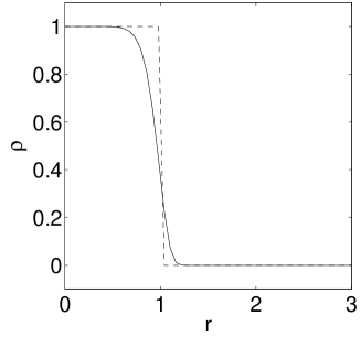
Figure 5: An illustration of the deformed top-hat defined in equation (31) for $\rho_{0}=1,\xi=1$. A top-hat density corresponds to an incompressible fluid and in standard GR gives the largest mass possible for a given proper angular radius. We slightly deform the top-hat to avoid numerical artifacts associated with discretization.

When we choose to solve for stars with fixed $\xi$ for several different core densities $\rho_{0}$, the proper radii of these stars will vary slightly. For linear stars, $R\simeq\xi$, and for non-linear ones we find that generically the angular radius is still similar to $\xi$, but a little larger.

We find numerically that for $R<<1$ we have very good convergence properties, but for $R>>1$ one requires extremely large numbers of grid points. However $\xi\sim 3$ is large enough for our purposes to see the 4-dimensional limit emerge. For $\xi\lesssim 3$ we find solutions in the non-linear regime approaching the limit of stability for a static star. We find that for the smallest stars tested, $\xi=0.3$, the code converges for configurations thought to be extremely close to the critical point, with photons emitted from the stellar core having redshifts of ${\cal Z}\simeq 15$. For the largest stars tested, $\xi=3$, the code converges for solutions with ${\cal Z}\simeq 2$, reaching at least $75\%$ of the estimated critical density.

4 Numerical Comparison with Linear Theory in the Low Density Regime

Detailed numerical tests and consistency checks of the non-linear method described above are presented in appendix 7. However a powerful independent test can be performed by simply comparing the solutions of the full non-linear scheme with those of the linear scheme, outlined in section 3.4. In the regime where the density perturbation on the brane is sufficiently small that the metric perturbation is much less than unity everywhere the two methods must agree.

The test is extremely valuable as the linear theory automatically satisfies the constraints and also has well understood asymptotic boundary conditions. The close agreement found, and described below, between the non-linear and linear methods in the low density regime indicates that both points are indeed satisfied well in the non-linear case. In addition, the non-linear method uses regularization for singular terms in $B$ at $r=0$, and the agreement implies the quality of this approximation is very good. Finally it means that finite boundary and resolution effects, which are inevitable in a numerical method, are likely to be small at the resolutions and lattice sizes used, and an estimate of absolute error in the metric functions and physical brane observables can be made from the comparison.

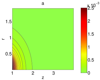
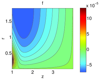
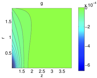
Figure 6: An illustration of the variable $a$ in the transverse traceless metric of the linear theory, and coordinate transform functions $f,g$ for a solution with $\xi=0.3$ generated using the linear method. The core density is chosen to be $\rho_{0}=0.1$. The decay of $a$ to zero away from the brane is clearly seen. The boundary conditions for $f,g$ are also clear; $f=0$ at r = 0 and on the large $z$ boundary, $g=0$ at large $r$, and $f,g$ are fixed on the brane by the matter. Figure 7 then displays the result of this coordinate transform to the metric of form (14), allowing comparison with the non-linear method. (lattice: $dr=0.02$, $r_{\rm max}=2$, $dz=0.005$, $z_{\rm max}=4$)

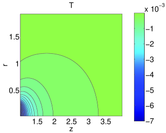
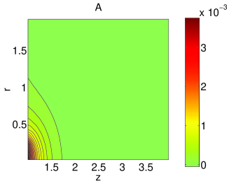
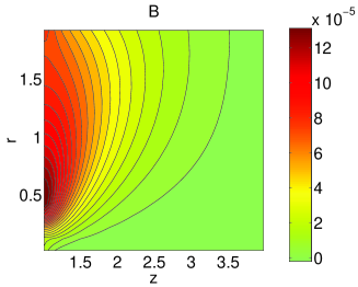
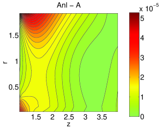
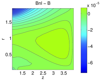
Figure 7: Upper plots; An illustration of $T,A,B$ generated from the linear method, for $\xi=0.3$, $\rho_{0}=0.1$ with $a,f,g$ shown in figure 6. The form of the functions agrees extremely well with the non-linear method (see for example the later figure 10). In particular we see that the metric functions do indeed decay towards the asymptotic boundaries, as we require in our non-linear boundary conditions. Note that the function $B$ is much smaller in magnitude than the other functions $T,A$. Although $B$ appears not to decay at large $r$, in fact it is so small everywhere, that at the large $r$ boundary it is of the same magnitude as the decayed $T,A$. The smallness of $B$ implies that the spatial geometry of the metric is effectively described as a conformal deformation of hyperbolic space by a factor $e^{2A}$. Lower plots; The full non-linear method was used to calculate solutions for the same brane matter, and the difference in the metric functions is shown. The density is sufficiently small that the non-linear method should reproduce the linear solution as $T,A,B<<1$. The non-linear method gives the quantities $Tnl,Anl,Bnl$ as a solution. The agreement is extremely good. For $T$ the peak deviation is only $\simeq 4\%$ of the peak value of the function. For $A$ this difference is even less at $\simeq 1\%$. For $B$ the difference is again very small for the lower half range of $r$. Near the maximum $r$ boundary the error becomes larger but as $B$ is so small, the absolute differences are tiny. The remarkable agreement between linear and non-linear shows that the boundary conditions imposed for the non-linear elliptic relaxation are indeed reproducing the asymptotic AdS geometry well. The following plot shows some brane observables calculated from the matching conditions and these have similar, if not even better agreement.

We calculate a solution using the full non-linear method for the smallest sized star considered elsewhere in this paper, with $\xi=0.3$. A sufficiently small energy density $\rho_{0}=0.1$ is chosen so that the metric perturbations are everywhere small. The lattice size and resolution are the same as used in later sections of the paper which examine the physical behavior of small stars. Thus estimates of error calculated here are directly applicable to later results. Figure 6 shows the functions $a,f$ and $g$ of section 3.4, calculated for the same size and density of star. The functions $T,A,B$ are given in figure 7, the bottom row showing the numerical difference between the two methods for the metric functions. The agreement is strikingly good. The functions $T,A$ agree extremely well, the maximum difference being for $T$, occurring at the core of the star, the fractional difference between the linear and non-linear methods being only $4\%$. For $A$ the difference is less at only $1\%$. Although the relaxed function $B$ is set to zero at the large $r$ boundary in the non-linear method, and from the linear method we see this is not quite true, we find that the magnitude of $B$ is much less than that of both $T,A$ and this tiny absolute difference appears to have no effect on the solutions in the interior of the lattice. This is very strong evidence that the non-linear method is indeed finding the correct physical solution and the boundary condition are effective. Furthermore the error for $B$ at small $r$ is tiny and indicates that the singular term regularization scheme (section 3.7) performs extremely well.

A further check is to compute the actual density and induced density and Weyl curvature component for the two solutions. The actual density is enforced as a boundary condition in the non-linear method. For the linear method it is implemented as a boundary condition for $a$, but the density plotted is computed from the brane matching conditions after the coordinate transform to the gauge (14). Hence we can see small finite boundary effects. The induced density is that required to support the induced 4-dimensional geometry in standard GR, and is therefore the $tt$ component of the Einstein tensor of the induced metric, given explicitly in appendix 8.1. The induced Weyl component is similarly a measure of curvature of the induced metric, detailed in the same appendix. Such induced quantities are extensively used in this paper to compare a 4-dimensional effective theory with actual 5-dimensional solutions. These quantities are plotted in figure 8 and excellent agreement is found between the two methods. An interesting point is that the density in the linear method is a little distorted at large $r$ due to the presence of the boundary. This does not appear to effect the interior solution which indicates that small boundary effects do not degrade the solution significantly. For all these quantities, differences in the core values of $\sim 1\%$ are found between the methods.

Finally, in figure 9 we plot some of the same quantities for a star with $\xi=3$, the largest size of star considered in this paper, again using the same resolution and lattice size as are used later in the paper. The $T,A,B$ metric functions are compared on the brane, the location on the lattice where the two methods give the greatest difference. Also the induced density is plotted. Excellent agreement is again found between the methods, particularly in the induced density, where differences of only $\sim 3\%$ are found. For the metric functions themselves, maximum differences of $\sim 10\%$ are seen relative to the peak values of the functions.

To conclude, in the low density regime the non-linear method performs extremely well at the resolutions and lattice sizes used in this paper. Comparison with the linear theory shows that the constraints are correctly imposed and the asymptotic geometry is indeed that of AdS at the horizon, consistent with the linear theory analysis of section 3.5. This also implies that our method to implement the singular terms at the $r=0$ axis in the elliptic relaxation works extremely well, as we see no obvious artifacts associated with $r=0$ in the comparisons. The maximum differences in the metric functions for small and large stars are $\sim 4\%$ and $\sim 10\%$ respectively at the star cores. Much smaller errors are found in actual brane observables, such as induced density and redshift, which we will in fact be using later, with typically $\sim 1-3\%$ differences for both small and large stars.

   

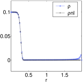
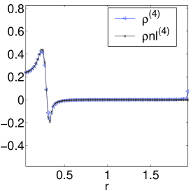
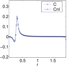
Figure 8: An illustration of the density, induced density and induced Weyl component on the brane generated from the linear method, for $\xi=0.3$, $\rho_{0}=0.1$, as in figures 6 and 7. On the left, the density is calculated from the brane matching conditions. In the non-linear method (here ${\rho}nl$) the density profile is an input boundary condition. For the linear method ($\rho$ in the figure) the density is less direct as an input. The middle plot shows the effective 4-dimensional density on the brane, ie. the density required to produce the induced 4-geometry actually found in the 5-dimensional solution. The rightmost plot shows the 4-dimensional Weyl component of the induced metric, as described in appendix 8.1. This gives a measure of the curvature on the brane. In all the linear quantities shown, we see that there are errors at the large $r$ boundary, although such errors are not so noticeable in the non-linear solution. We expect such errors from the finite size lattice and note that the errors appear to have no physical effect on the inner points where extremely good agreement is found between the linear and non-linear methods, the deviations being hardly visible on the plots and the maximum differences being of order $1\%$ of the typical core values.

 

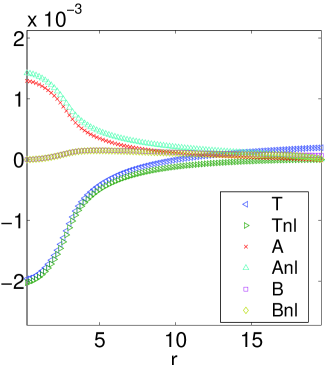
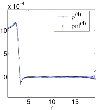
Figure 9: On the left, the metric functions $T,A,B$ are shown, now just on the brane, for the linear and non-linear methods for a large star, $\xi=3$, $\rho_{0}=0.001$. The density is sufficiently small that the linear method should reproduce the non-linear method solutions. $Tnl,Anl,Bnl$ are quantities from the non-linear method, $T,A,B$ are from the linear. The maximum differences for the linear and non-linear are on the brane itself, as for the small star case shown in the earlier figure 6. We see that the peak differences at $r=0$ are $10\%$ for both $T$ and $A$ compared to the peak function values themselves with very small absolute difference for $B$. Thus the agreement between the non-linear and linear method in this low density regime is again extremely good, for large stars as well as small. Whilst the function $T$ is a coordinate scalar for static spherical geometries, $A,B$ are not. An example of another coordinate scalar is the 4-dimensional effective density. This is the density profile that would reproduce the induced geometry in a purely 4-dimensional theory. The non-linear ${\rho}nl^{(4)}$ and linear $\rho^{(4)}$ are plotted for the same solution and again very good agreement is found, $\sim 3\%$ peak difference compared to peak value. (all lattices: $dr=0.2$, $r_{\rm max}=20$, $dz=0.03$, $z_{\rm max}=46$)

5 Physical Solutions and Results

Appendix 7 shows in detail that the method outlined does indeed solve the Einstein equations to a good accuracy using the resolutions and lattice sizes considered in this paper. The previous section 4 shows that in the low density regime, the non-linear method very closely reproduces the linear theory results which can be numerically computed by a simpler, independent method. Confident that the method gives solutions of good quality, allowing physical tests and comparisons to 4-dimensional effective theory, we now proceed to investigate the non-linear behavior of Randall-Sundrum stars.

Firstly we study small stars, showing typical solutions for $\xi=0.3$ (so $R$ is several times less than the AdS length, $l=1$, in our units), describing their geometry and showing the upper mass limit is reproduced. These are the first calculations of high energy density non-linearity on branes, from localized matter. We expect that the qualitative phenomenon found here, are not specific to the Randall-Sundrum model. Then large stars are considered, results being shown for $\xi=3$, so $R\simeq 3$, the largest sizes that could be relaxed in a reasonable time. The induced geometry on the brane is shown to be well described by a 4-dimensional effective theory. The confinement of the geometric deformation to the brane is then confirmed for both large and small stars, in both the linear and non-linear regime, consistent with a pancake like scaling predicted in [16, 7, 8]. In fact the degree of confinement is interestingly found to increase for highly non-linear stars near their upper mass limit, indicating non-linearity does effect the bulk geometry, even in the case of large stars. Finally we consider in detail how the transition to the 4-dimensional effective theory proceeds for increasing $R$.

5.1 The Geometry of Small Stars

(Some results presented in section 2, ‘Highlights of Results’)

In this section we consider stars generated with a density profile of coordinate radius $\xi=0.3$, a few times smaller than the AdS length. We present a series of configurations, all of the same $\xi$, ranging from the linear to the non-linear regime, the most non-linear example being the densest star we could numerically compute for $\xi=0.3$ with proper radius $R=0.38$. As we shall see, it is a highly relativistic object, the numerical method performing most stably for small stars.

We start by showing the form of the metric for the most non-linear solution corresponding to a core density $\rho_{0}=7.0$, which is larger than the brane tension, $\sigma=6$. The metric functions are shown in figure 10. The most striking feature is that the configuration shows confinement of the perturbation, just as for the linear solutions (the metric functions of less dense stars also with $\xi=0.3$ are found in figure 7 of section 4 and figure 22 in appendix 7). The metric function $B$ is much smaller than the other two functions and thus, from the metric (14), the spatial sections are well approximated by a conformal deformation of those of AdS. The metric function $T$ has a peak magnitude of $2.5$, greater than one, giving rise to large redshift effects. The peak value of $A$ is still less than one, indicating the non-linearity is less pronounced in the spatial perturbations. In figure 11 we obtain a measure of the curvatures on the brane by plotting the scaled Weyl components given in appendix 8.1 for the most non-linear configuration. It is clear that the curvatures generated in the solution are large, even compared to the bulk Ricci scalar, $|{\cal R}|=20$.

     

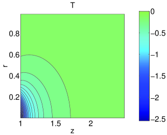
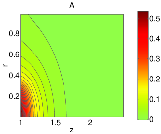
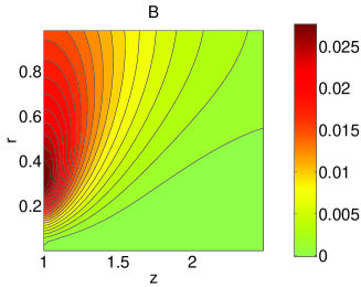
Figure 10: An illustration of the metric functions $T,A,B$ for a configuration with $\xi=0.3$ and core $\rho_{0}=7.0$. This is an extremely relativistic ‘micro-star’, whose proper angular radius is $R=0.38$, approximately a third of the AdS length. The core value of the metric function $T=-2.5$ corresponds to a redshift of ${\cal Z}=12$ for photons created in the star core traveling to $r=\infty$ in the brane. The metric function $B$ is much smaller than $T$ and $A$ indicating the spatial sections are approximately conformal to those of AdS. In addition, the maximum of $|A|$ is considerably less than that of $|T|$ indicating the red-shifting effects are more pronounced than spatial deformations from the unperturbed AdS. The solution is thought to be close to the upper mass limit which appears to be present for both small and large stars. The value of $\rho_{0}$ is actually slightly larger than the brane tension $\sigma=6$. (lattice: $dr=0.02$, $r_{\rm max}=2$, $dz=0.005$, $z_{\rm max}=4$)

  

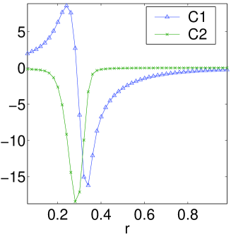
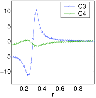
Figure 11: An illustration of the Weyl components (defined in appendix 8.1) calculated on the brane for the same configuration as in figure 10. The curvatures measuring up to $\sim 10-15$ are comparable to the characteristic curvature from the negative bulk cosmological constant which gives a Ricci scalar $|{\cal R}|=20$.

The form of the density profile is an input to the solution, and from the remaining brane matching conditions we can extract the pressure on the brane. There are two components of pressure, the radial and angular components, but the boundary condition of isotropy ensures that these are equal. Figure 12 shows the pressure calculated for various density profiles, each with $\xi=0.3$ but with different $\rho_{0}$. The solutions range from the near linear where $P<<\rho$ to the highly non-linear where $P>>\rho$. The most nonlinear solution that was relaxed (corresponding to the solution in figure 10) is plotted and gives an extremely large central core pressure, with $P/\rho\simeq 5$.

     

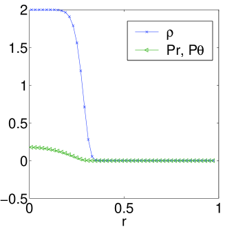
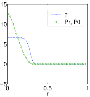
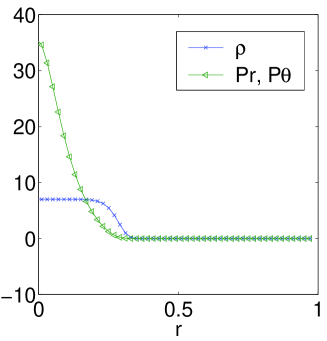
Figure 12: An illustration of $\rho,P_{r},P_{\theta}$ for configurations with $\xi=0.3$. The core densities $\rho_{0}=2.0,\,6.6,\,7.0$ from left to right. The lowest density, still relatively large compared to the brane tension $\sigma=6$, yields a pressure visibly much smaller than the density. The middle and right solutions have core pressures larger than the core density indicating the extreme non-linearity of the solutions. Note that for just a $6\%$ change in density from $\rho=6.6$ to $\rho=7.0$ the core pressure over density increases by a factor of $\sim 2.5$. The density and pressures are measured from the brane matching conditions. Whilst the density is input as a boundary condition, the pressures are derived from the solution. The isotropy boundary condition functions well, the radial and angular pressure components being indistinguishable in such a plot. (all lattices: $dr=0.02$, $r_{\rm max}=2$, $dz=0.005$, $z_{\rm max}=4$)

The limiting behavior can be seen by plotting the ratio of core pressure to density against the core density. In the Newtonian theory there is a quadratic dependence of the pressure on the density. In figure 1 (found in the ‘Highlights of Results’ section 2), we explicitly see a departure from the linear dependence of $P/\rho$ on $\rho$, which holds for very low densities. Instead we find diverging behavior as $\rho_{0}\rightarrow 7$. For stars with higher core density, no convergent numerical solution was found. The apparent divergence in $P/\rho$ strongly suggests that the reason we cannot relax denser stars is that the static solutions do not exist, in analogy with the 4-dimensional case. Thus even for small stars we have the same qualitative behavior of an upper mass limit as in standard GR. The task of investigating the dependence of the limiting mass on radius for $R<<1$ is left for future work, and may have interesting implications for micro black hole formation.

For the purposes of this paper we are primarily interested in how closely the induced brane geometry is described by a purely 4-dimensional local description, and therefore we wish to calculate intrinsic properties of this brane geometry. The intrinsic metric on the brane at $z=1$ is,

$$ds^{2}_{\rm induced}=\left.-e^{2T(r,z)}dt^{2}+e^{2\left(A(r,z)+B(r,z)\right)}dr^{2}+e^{2\left(A(r,z)-B(r,z)\right)}r^{2}d\Omega_{2}^{2}\,\right|_{z=1}$$ (33)

and then we may calculate a complete set of induced 4-geometric quantities such as the Einstein tensor and the Weyl tensor which together specify the geometry. In 4-dimensions with static spherical symmetry there is one independent Weyl component and 3 Einstein tensor components. We characterize the Einstein tensor components in terms of the effective density, $\rho^{(4)}$, radial pressure, $P_{r}^{(4)}$, and angular pressure component, $P_{\theta}^{(4)}$, that would result in such a geometry for 4-dimensional gravity. Their explicit form is given in appendix 8.1. This is a useful characterization of the curvature as, later, in the large star case, we see that the induced density and pressure agree with the actual quantities calculated from the brane matching conditions. Another quantity we compute is the metric component $T$, which due to the static symmetry is a scalar function under $r,z$ coordinate transformations. Thus for static configurations the redshift, ${\cal Z}$, of photons emitted from the core of a star to infinity on the brane,

$$e^{-T(r=0,z=1)}=1+{\cal Z}$$ (34)

is a well defined physical quantity. Such intrinsic quantities are plotted for the most non-linear solution with $\xi=0.3$, and are found in figure 13. We see that the induced density and pressure have similar forms to the 5-dimensional quantities but have approximately twice the value.

 

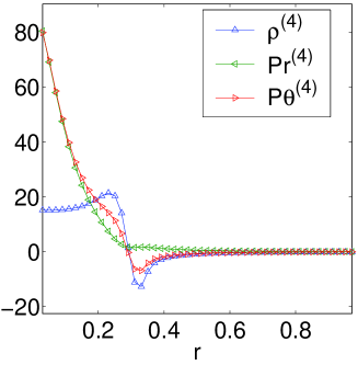
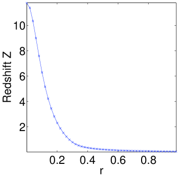
Figure 13: On the left, an illustration of induced $\rho^{(4)},P_{r}^{(4)},P_{\theta}^{(4)}$ for the $\xi=0.3$, $\rho_{0}=7$ solution shown in figure 10. The curves have a similar qualitative form to the right hand plot of figure 12, the actual 5-dimensional density and pressures for the solution, but quantitatively deviate by a factor $\sim 2$. As we expect, 4-dimensional gravity does not describe the 5-dimensional induced geometry well for small stars. On the right, for the same solution an illustration of the redshift of photons emitted from coordinate position $r$ on the brane and observed asymptotically at large $r$ on the brane. The redshift of photons emitted from the stellar core is ${\cal Z}\sim 12$ indicating the extremely relativistic nature of this ‘micro-star’ solution.

The largest metric deviation is in $T$. This is best characterized in terms of the core redshift of photons which gives a value of ${\cal Z}\simeq 12$, indicating the non-linearity of the solution. The spatial curvature of the metric is large too. A striking feature of the solutions is that the metric function $B$ is very small compared to the other two functions. If we now approximate $B\sim 0$ then the spatial metric becomes,

$$ds_{\rm spatial}^{2}=e^{2A}\frac{1}{z^{2}}\left(dr^{2}+r^{2}d\Omega^{2}+dz^{2}\right)$$ (35)

which just corresponds to a conformal transformation of flat sliced hyperbolic space. This allows us to understand the spatial geometry by considering the metric function $A$ in figure 10 as this conformal factor. The positive $A$ implies that the volume in the bulk near the star on the brane is ‘more’ than in the unperturbed case. This indicates that the solution does not pinch off the portion of the brane containing the matter, an idea illustrated in figure 14. We more rigorously show this by plotting, in figure 15, the geodesics of this spatial geometry which are symmetric about $r=0$. The relevant AdS spatial geodesics are circles centered on $z=0$ in these coordinates. We see the actual distortion of the geodesics from the non-linear curvature. The proper distance of the curved geodesics does indeed increase monotonically for increasing $r$ intersection with the brane indicating that no pinching or geometric pathologies are occurring.

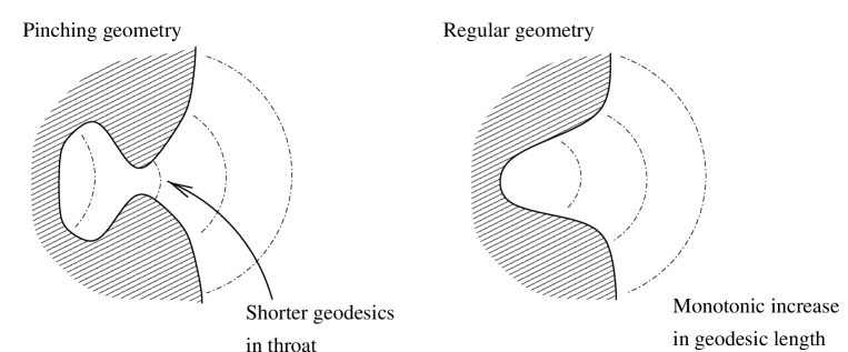
Figure 14: A schematic illustration of a brane ‘pinching off’ a stellar region. Plotting the length of symmetric spatial geodesics against radial coordinate distinguishes the left-hand from the right-hand cases. A pinched geometry could lead to pathologies at finite stellar density, the matter region becoming entirely trapped. Instead we find our solutions have monotonically increasing spatial geodesic length corresponding to the right-hand case.

         

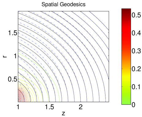
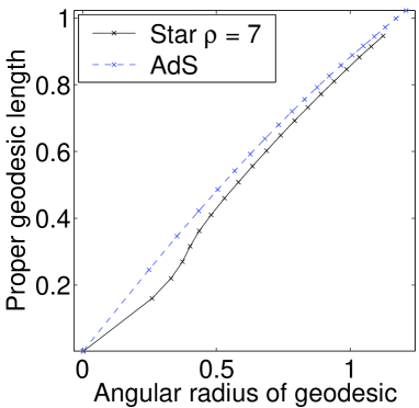
Figure 15: An illustration of spatial geodesics for the solution $\xi=0.3$, $\rho_{0}=7$ shown in figure 10. Note that the geodesics (blue and black) are superimposed on a contour plot of the metric function $A$ (red - green). As the metric function $B\sim 0$ the spatial geometry is simply conformal to hyperbolic space, the conformal factor being $e^{2A}$. The dotted blue lines are the AdS geodesics, which are simply circles centered on the boundary $z=0$ in these coordinates. The black solid lines are the geodesics calculated for the star geometry. We see clear deviations in the star geometry from the unperturbed AdS. The right plot shows the path length against proper angular radius of interception with the brane. The function is smooth and monotonically increasing indicating that there is no ‘pinching’ off of the section of the brane containing the star.

5.2 The Geometry of Large Stars

We now consider the geometry of the largest stars relaxed, having coordinate size $\xi=3$, the characteristic proper radius being a little larger, and therefore several times the AdS length. For these larger stars we were able to relax configurations with core redshifts of ${\cal Z}\simeq 2.1$. The key result of this section is that for large stars, the effective theory on the brane is indeed 4-dimensional General Relativity even when the configuration becomes non-linear.

Note that ${\cal Z}\simeq 2.1$ is not as close to the upper mass limit as for the densest small star of the previous section. For higher densities the numerical scheme gave no convergent solution, although this is almost certainly an artifact of the scheme and not an indication that higher density solutions do not exist. We later estimate that the ${\cal Z}\simeq 2.1$ solution has a core density that is $\sim 75\%$ of the top-hat upper limit for its proper radius.

Figure 16 shows the metric functions for the most dense star relaxed. We see that as for the small stars, again the function $B$ is very small compared to $T,A$. $T$ is large in value, reaching a peak on the brane at $r=0$ of $|T|\simeq 1.1$. The form of the metric functions appears qualitatively similar to those of the small stars, although less localized in the $r$ direction. This is to be expected from the linear theory [7], which shows that the asymptotic behavior of the propagator on the brane is $\sim\frac{1}{r^{2}}$ at small scales and $\sim\frac{1}{r}$ for large. Again the metric functions are localized in $z$. In fact $A$, whilst positive near the brane, falls off quickly and becomes slightly negative (just visible in the plot), before asymptotically decaying to zero, consistent with the asymptotic behavior predicted in the linear theory (49). The relation between the typical proper distance that the metric functions protrude, and the stellar radius $R$, is discussed later in section 5.3. For the linear stars we expect such localization, but the configuration shown is not a small perturbation and again localization is exhibited. The 5-dimensional Weyl components are plotted in figure 17 to show the magnitude of the characteristic curvature which is seen to be much less than the AdS curvature scale. To recover 4-dimensional effective behavior non-linearly it is crucial that the characteristic scales of the solution are insensitive to the 5-dimensional scale, and this is exactly what is seen here.

   

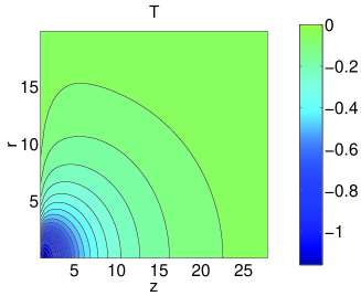
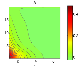
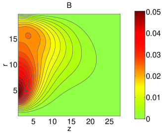
Figure 16: An illustration of $T,A,B$ for a large star with $\xi=3$ and $R=3.7$. The core density $\rho_{0}=0.15$ corresponds to the densest star our method relaxed stably for this $\xi$. We later compute that this core density is at least $75\%$ of the top-hat upper limit for a star of such a radius. Again the characteristic $z$ confinement of $T$ and $A$ is seen. A reduced $z$ range is plotted for $A$ to graphically resolve the detail. As with the small stars, $B$ is much smaller than $T,A$ and indicates that the spatial geometry is simply conformal to flat sliced hyperbolic space. The maximum perturbation from AdS appears in $T$ where a peak value of $|T|\simeq 1.1$, which gives rise to a redshift of ${\cal Z}\simeq 2.1$ for photons emerging from the core to infinity on the brane. This is not a small perturbation and is later (section 5.4) shown to be beyond the reach of higher order perturbation theory. Note that the $z$ depth of the lattice is actually $z_{\rm max}=46$ in order to ensure the asymptotic behavior is good (only $z<25$ is actually plotted). Thus many points are required in the z-direction to maintain AdS length resolution. (lattice: $dr=0.2$, $r_{\rm max}=20$, $dz=0.03$, $z_{\rm max}=46$)

  

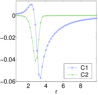
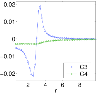
Figure 17: An illustration of the Weyl components $C1,C2,C3,C4$ (described in appendix 8.1) on the brane. These indicate the magnitude of the curvature perturbation. For the small stars the densities and curvatures are large compared to the brane tension and unperturbed AdS curvature. Now for large stars both the density ($\rho_{0}=0.15$) and typical curvature is small compared to the fundamental bulk and brane scales. This implies that the solution, whilst non-linear, does not probe the scales associated with the higher dimensions, the metric functions remaining bounded and well behaved. If a 4-dimensional effective theory is to be reproduced, this separation of curvature scales between the fundamental ($\Lambda,\sigma$), and star matter scales ($\rho_{0}$, $R$), should be observed for large objects. (lattice: $dr=0.2$, $r_{\rm max}=20$, $dz=0.03$, $z_{\rm max}=46$)

Now we examine the intrinsic geometry on the brane itself. Figure 18 shows the 4-dimensional induced density, and radial and angular pressures that would give rise to such an induced metric configuration in 4-dimensions. Plotted with them are the actual 5-dimensional density, an input for the system, together with the 5-dimensional pressure measured from the brane matching conditions. We see extremely close agreement for both linear and non-linear stars. The degree of non-linearity can be seen in the rightmost plot as the pressure is becoming large compared to the density. For this large star the agreement is striking. Of course linear theory states that a 4-dimensional intrinsic behavior should be observed. A key result of this paper is that this applies far beyond the linear regime. In the graphs we see that the agreement between the actual 5-dimensional density and the 4-dimensional effective density appears approximately independent of the density over the range tested. This is seen more clearly in figure 2 of the ‘Highlights of Results’ section 2 and in section 5.4.

     

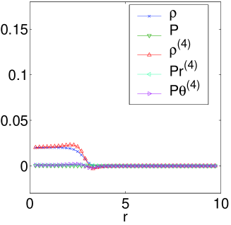
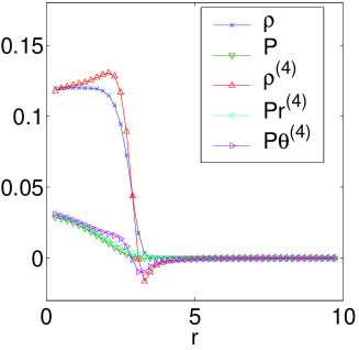
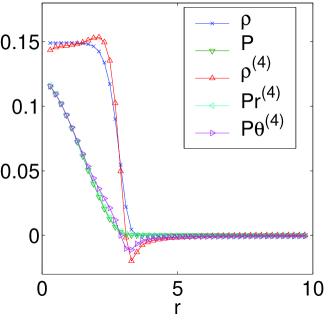
Figure 18: An illustration of actual density and pressure $\rho,P$ together with 4-dimensional effective density and pressure $\rho^{(4)},Pr^{(4)},P\theta^{(4)}$, for $\xi=3$ large stars with various core densities, $\rho_{0}=0.020,0.120,0.149$ from left to right. The actual density and pressure are calculated from the brane matching conditions. Note that isotropy is maintained as a boundary condition and the two pressure components $Pr,P\theta$ are equal to high precision, plotted here as simply $P$. Moving from the linear (left) to non-linear (right) we see the pressure becomes significant compared to the density. The key result of the plot is the small differences found between the actual and effective quantities. The effective quantities are the density and pressure components required to derive the induced brane geometry in 4-dimensional GR. We see extremely close agreement between both the density and pressure components of the actual 5-dimensional solution and the effective theory. Note that isotropy is not input into the induced pressure components which are simply calculated here from the induced metric, yet $Pr^{(4)}\simeq P\theta^{(4)}$ is indeed found. For linear configurations it is expected from theory that the 5-dimensional solution on the brane looks 4-dimensional. However the key result of this paper is that even for highly non-linear solutions, (the rightmost plot), the agreement with a 4-dimensional effective theory is just as good. This is further characterized in the section 5.4 and in the ‘key results’ figure 2. (all lattices: $dr=0.2$, $r_{\rm max}=20$, $dz=0.03$, $z_{\rm max}=46$. no extrapolation to $dz=0$ is performed leading to a maximum $\sim 4\%$ systematic in $\rho^{(4)}$, estimated by comparison with $dz=0.05$)

5.3 Non-Linear Confinement

We now examine the transverse extent of the solutions. The function $T$ is a scalar under residual coordinate transformations which preserve the static spherical symmetry of the metric. The value of $T$ decays asymptotically to zero along the axis $r=0$ away from the brane, having its largest magnitude at (for small stars), or near (for large stars) the brane. Photons emitted at the core of the star may propagate along this axis. A static observer at some point on this line will then observe a redshift in the received photons. We could characterize the geometry by considering the proper distance along the line $r=0$ for the redshift to take a certain value. For convenience, we equivalently choose to consider the point where the value of $T$ is a half that on the brane. This is a unique point for all the configurations tested and characterizes the confinement of the perturbation to the brane.

The first plot in figure 19 shows how the extent of the star depends on its angular radius on the brane. The stars shown are all in the linear regime. Several low density solutions are used to extrapolate results to zero core density. We see an approximately linear relation over the range of $\xi$ tested. At larger $\xi$, the relation deviates from linear, appearing to become flatter, consistent with the ‘pancake’ scalings predicted in [7, 16]. Thus the characteristic fall off distance of the redshift along the axis increases for increasing star radius. The larger the star, the shallower this function is as it decays away from the brane. This is to be expected as the asymptotic behavior of the Greens function clearly depends on the radial scale probed. Numerically this slow fall off is a reason that very large stars are difficult to simulate. One requires very large physical lattice size in the $z$ direction whilst maintaining resolution better than the AdS length.

The remainder of the graphs show the variation of this confinement distance with increasing density for a fixed $\xi$. The smallest stars simulated, with $\xi=0.3$ relax with the greatest degree of non-linearity. For these we see the very interesting feature that the confinement distance first increases in the linear regime as the density, and thus core $|T|$, increases, but then begins to decrease as the configuration becomes highly non-linear. As discussed earlier, fixed coordinate $\xi$ does not fix the angular radius of the star, which is also plotted in the figure and is seen to monotonically increase with core $|T|$. Thus for the linear configurations, where $|T|<<1$, the increase in confinement distance follows the radial increase in star size on the brane as one would expect. However the decrease in transverse extent for the very dense stars appears to be a significant and purely non-linear effect. For the most non-linear star tested, $\xi=0.3$ and this extent is $\simeq 75\%$ of the zero density one with the same $\xi$, whilst the angular radius is $\simeq 25\%$ larger. It is important to note that the absolute extent of the star clearly does not decrease, but rather the decay distance decreases implying the function $T$ falls more steeply near the brane for very non-linear configurations than for linear ones.

The maximum density star for $\xi=0.3$ is very close to what appears to be a critical mass limit, as discussed in section 5.1. However with the solutions available, we cannot determine whether the transverse size actually tends to zero at the critical point, or whether it remains finite. For the larger stars we are unable to probe so far into this non-linear regime for reasons of numerical stability, but the same curves for $\xi=1.5,2,3$ stars are plotted, where qualitatively the behavior appears to be similar over the range of core redshifts available. Again the turn around in transverse extent is observed for the more non-linear stars where the angular radius remains increasing, the turn around points being at approximately the same value of core $|T|$ as for the $\xi=0.3$ case. The densest $\xi=3$ star has approximately the same confinement distance as a zero density star of the same $\xi$, but has a proper radius $\sim 30\%$ larger. Thus this confinement distance dependence on density does not appear to become less pronounced with increasing $R$. It would be very interesting future work to see the scaling of this effect for very large stars, if such solutions could be computed.

The fact that this behavior is still seen for non-linear $\xi=3$ stars is important. As we have seen in section 5.2, non-linearity does not introduce AdS scale curvature perturbations into the large star bulk geometry. The source length scale and AdS length scale remain separated. However, we see here that the non-linearity does change the nature of the bulk geometry, though the modification of behavior appear to be only on large wavelengths. Despite the non-linearity modifying the bulk response, the 4-dimensional effective GR description appears to hold as well for the large non-linear stars as for the linear ones.

It is worth noting that if the confinement distance does go to zero at the upper mass limit, as is possibly indicated in the $\xi=0.3$ behavior, then the same may also occur for large stars extremely close to the upper mass limit. This zero confinement distance would indicate that the AdS length scale was entering the geometry of the perturbation to the bulk, and would give rise to a deviation from 4-dimensional behavior in the induced geometry. Presumably for very large stars one would have to be extremely close to the critical point in order to see such effects.

The increase in confinement is reminiscent of the change in the sense of deflection of the brane, relative to the ‘Randall-Sundrum’ transverse-traceless gauge coordinates in the linear theory. This would occur if the sign of the trace of the stress energy changes, as happens for incompressible fluid matter in the strong gravity regime. Thus, although there is no ‘radion’ in the one brane case at low energies [19], one can heuristically think of this confinement of the perturbation as an analogous, although non-dynamical, quantity. Furthermore, this would confirm the suspicion that for very large stars, the normalized confinement of figure 19, would indeed change by an order one amount, for strong gravity configurations, where all curvatures remain small.

   

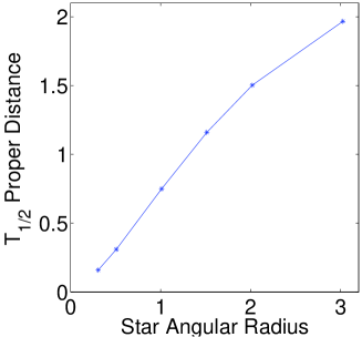
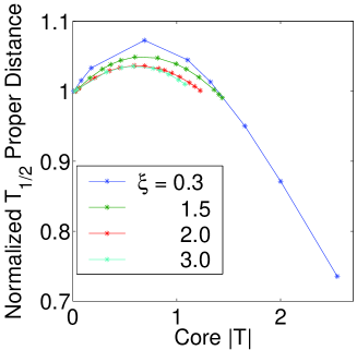
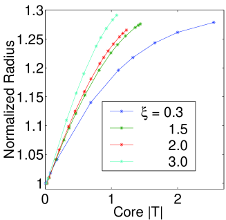
Figure 19: An illustration of confinement for various star radii. The left plot is of proper distance along the axis $r=0$ to $T_{1/2}$, the point where $T$ takes half the value it has on the brane, against the proper star radius. The results plotted are extrapolated to stars of zero density. The middle plot then shows how the same quantity changes with increasing density, the core value of the metric function $T$ being the measure of the geometric response to this density. Curves are plotted for different $\xi$, and the $T_{1/2}$ distance is normalized using the zero density values of the leftmost plot. The smallest stars relaxed have the highest non-linearity and we observe first an increase in $T_{1/2}$ distance, with increasing core $|T|$, and thus density, and then a decrease for larger densities. The increase is expected as the proper radius, plotted in the right-hand graph (normalized by $\xi$), is increasing monotonically for increasing density - note, the coordinate width of the density profile, $\xi$, is fixed in these solutions but the actual proper angular size then must be found from the solution itself. The leftmost plot shows exactly this increase of $T_{1/2}$ distance for increasing radius. However the decrease in $T_{1/2}$ distance for high core $|T|$ is not expected and indicates that the physical perturbation is becoming more peaked near the brane for higher density stars. This appears to be a purely non-linear effect. With the solutions available for $\xi=0.3$, it is unclear whether the $T_{1/2}$ distance reaches zero at finite $T$, asymptotically at the upper mass limit, or not at all. This remains an interesting topic for future work. The larger stars, whilst further from their upper mass limit, still show similar behavior, the peak value of the $T_{1/2}$ distance being at approximately the same core value of $|T|$, or alternatively core redshift. We conclude that the confinement of the physical solutions in fact increases near the upper mass limit, even for large stars. It implies that non-linearity does effect the geometry of the bulk perturbation for large stars, although the modification from linear behavior only occurs on long wavelengths. (lattices: $\xi=0.3$: $dr=0.02$, $r_{\rm max}=2$, $dz=0.005$, $z_{\rm max}=4$, $\xi=1.5$: $dr=0.10$, $r_{\rm max}=10$, $dz=0.02$, $z_{\rm max}=21$, $\xi=2.0$: $dr=0.15$, $r_{\rm max}=15$, $dz=0.02$, $z_{\rm max}=31$, $\xi=3.0$: $dr=0.20$, $r_{\rm max}=20$, $dz=0.03$, $z_{\rm max}=46$.)

5.4 Upper Mass Limits and 4-dimensional Effective Theory

(Some results presented in ‘Highlights of Results’ section 2)

In the previous section 5.2 we observed that 4-dimensional behavior was recovered on the brane for relativistic large stars with $\xi=3$. In this section we characterize the transition from 5-dimensional to effective intrinsic 4-dimensional behavior.

In order to compare like with like, we use the 5-dimensional solutions to generate 4-dimensional density profiles as a function of proper distance in the induced geometry. Assuming isotropy we numerically integrate the 4-dimensional Einstein equations given in appendix 8.1 using this generated density profile with the relevant boundary conditions for asymptotic flatness at large $r$. The parameters we compare to the actual 5-dimensional solutions are the core value of $T$, related to the redshift of photons from the star’s core, and also the core pressure. With the static, spherical symmetry both these quantities are coordinate scalars under the $r,z$ coordinate freedom. Note that obviously the core density agrees by construction.

In figure 2 (found in the ‘Highlights of Results’ section 2) we plot the deviation of these quantities in the 4-dimensional effective theory from the actual measurements made on the 5-dimensional solutions. Three sets of stars are shown with different $\xi$. For each set a range of core densities are presented. The lattices used are generated at two values of $dz$ and quadratic extrapolation is used to calculate the $dz=0$ continuum value, as described in appendix 8.3.

The results are striking. We have already seen that the $\xi=3$ stars give good agreement with the 4-dimensional Einstein equations acting on the induced metric. This is again observed in these plots, where the actual 5-dimensional quantity is plotted against the induced effective 4-dimensional one, and the points for $\xi=3$ lie close to the $4d=5d$ straight line for both redshift and core $P/\rho$. $\xi$ is not the actual proper radius of the star, but rather a coordinate radius. However $\xi$ is approximately the proper radius, and this proper radius increases as one moves vertically down (to larger $\xi$) towards the $4d=5d$ line. Thus, the larger stars do lie nearer the $4d=5d$ line, indicating a better approximation by the 4-dimensional induced theory. This is true over the range of solutions, for both linear and non-linear densities. For finite sized stars, the effective theory consistently underestimates both 5-dimensional quantities plotted.

Furthermore the points for $\xi=3$ approximately lie on a straight line. For $\xi=3$ perfect agreement with the 4-dimensional effective theory is not expected as the proper radii are only between $3-4$ times larger than the AdS length. However the fact that the points lie on a straight line indicates that the degree of deviation from the intrinsic description appears to be independent of the non-linearity over the range of densities tested. We discuss this further shortly.

We also plot a line indicating the core redshift and $P/\rho$ for $\xi=3$, from 4-dimensional linear theory, integrated in a similar fashion to the 4-dimensional non-linear theory, using the same density profile. This is graphed against the non-linear 4-dimensional quantities to indicate the degree of non-linearity. Already for redshifts above $0.2$ we see that the linear and non-linear 4-dimensional theory have very poor agreement. In fact for the most dense $\xi=3$ configurations, the linear theory underestimates the core redshift and pressure by a factor of about three. Thus for the large redshift $\xi=3$ stars, the non-linear corrections to these linear quantities are much larger than the quantities themselves. Therefore the regime tested is fully non-linear, and as such, is far beyond the reach of second or higher order perturbation theory.

It is important to note that these quantities merely indicate an agreement of a global nature, and thus for completeness we also include figure 20. This confirms the intrinsic description gives an increasingly good approximation to the induced geometry locally, as the star radius increases, for both linear and non-linear core densities. Note also the previous figure 18 in section 5.2.

We see from the small stars, in section 5.1, that there appears to be an upper mass limit for a given radius, as in the 4-dimensional theory. For the larger stars our method currently does not allow us to stably relax configurations very near the critical mass. However, we infer this mass to be close to its value in the 4-dimensional theory as we see such close agreement leading up to the limit. For the most non-linear solution with $\xi=3$, the induced angular radius is $R=3.7$. The upper mass limit in 4-dimensional theory, derived for a top hat density profile, is given as $M_{\rm max}=8\pi\frac{4}{9}R$ in our units, which corresponds to $M_{\rm max}=41$, whereas the effective 4-dimensional mass computed for our most non-linear solution is $M=30$ which is approximately $\simeq 75\%$ of this 4-dimensional critical mass for this radius. Thus the density $\rho_{0}$ is similarly $\simeq 75\%$ of the critical density. Note that this 4-dimensional density limit will overestimate the 5-dimensional density limit for a star of this radius, as we have seen the effective theory underestimates the 5-dimensional core $P/\rho$. Thus the core density of this solution is at least $\simeq 75\%$ of the 5-dimensional density corresponding to the upper mass limit for a star of the same radius.

Agreement for large stars was expected for low densities. We also find it for high densities. We should not compare linear and non-linear stars of the same $\xi$ directly as these have different proper radii. Thus in figure 2, because the stars of the same $\xi$ have slightly varying proper radius, it merely allows us to say larger stars, both linear and non-linear, are better approximated by a 4-dimensional effective theory, since vertical lines in the figure approaching the $4d=5d$ line from above are increasing in proper radius. We must use different $\xi$ values to find stars with the same proper radius but different density. In figure 21 we do exactly this, and quantify how the core density effects the degree of agreement between the induced and actual brane quantities. In this figure, two stars of the same proper radius $\simeq 2$, are shown overlaid using a suitable normalization. One star is highly non-linear, near its upper mass limit with a core redshift of ${\cal Z}\sim 3$. The other is a low density solution. We see very similar induced profiles for both, after normalization by the actual core density, indicating that the approximation of the induced theory to the actual is roughly independent of the degree of core density of the star, over the density range tested. We find similar behavior for the induced pressures. Note that the confinement proper distance to $T_{1/2}$, discussed in section 5.3, is quite different for the two stars, being $1.15$ and $1.51$ for the high and low density stars respectively. Thus even though the 5-dimensional geometry is different near the upper mass limit than at low density, for a fixed proper radius, the induced behavior appears to be approximated by the 4-dimensional theory equally well.

   

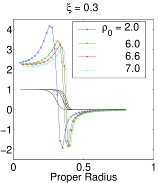
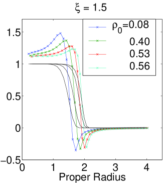
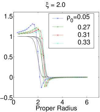
Figure 20: An illustration of induced density normalized by the actual density at the core as a function of proper radius on the brane for several values of $\xi$. Also plotted are the corresponding actual density profiles (in black), again normalized to unit value at the core. We see increasing agreement, for both linear and non-linear densities, between the actual and induced curves as $\xi$, and thus the proper radius of the star, increases. For each value of $\xi$ the lowest density star has a very small core redshift. The densest stars have the following core redshifts; $\xi=0.3$: ${\cal Z}=11.7$, $\xi=1.5$: ${\cal Z}=3.2$, $\xi=2.0$: ${\cal Z}=2.4$, all far into the non-linear regime. These profiles confirm the results of figure 2, showing the local agreement of quantities.

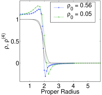
Figure 21: In this figure we compare a highly non-linear ($\rho_{0}=0.56$, the densest $\xi=1.5$ star available) and a low density star ($\rho_{0}=0.05$, $\xi=2.0$) with the same proper radius $\sim 2.0$. The induced (coloured) and actual (black) densities are plotted for both stars, normalized by the actual core density, as in the previous figure 20. The black curves, the actual densities, agree by construction, as a result of choosing stars with the same proper radius. The $\xi=1.5$ star has a core redshift of ${\cal Z}=3.2$, whilst the $\xi=2.0$ has ${\cal Z}=0.06$. Note also that the confinement proper distances are $1.15$ and $1.51$ for the $\xi=1.5$ and $\xi=2.0$ stars respectively. Despite one star being linear and the other highly non-linear near its upper mass limit, the denser one being considerably more confined to the brane, the similarity between the induced curves shows that this has little effect on the degree of approximation of the effective theory.

6 Conclusion

We have outlined a scheme which allows the full non-linear Einstein equations to be numerically solved elliptically for Randall-Sundrum gravity, with static, spherically symmetric matter on the brane, giving rise to regular 5-dimensional solutions with axial symmetry. Radiation boundary conditions imply that the horizon geometry is that of AdS. Due to the elliptic nature of our scheme, the method allows both an asymptotically AdS horizon geometry, and the brane matching relations to be simultaneously imposed as boundary conditions. We explicitly show that data specifying a star geometry in 4-dimensions uniquely determines the full 5-dimensional bulk solution.

Using this numerical scheme we study small and large stars in Randall-Sundrum gravity. Highly non-linear configurations are calculated for small stars, whose radius is less than the AdS length, having core red-shifts up to ${\cal Z}\simeq 12$. An upper mass limit is found that is qualitatively similar to that in 4-dimensions, implying that the brane does not stabilize highly non-linear static configurations. No pathologies are found in the spatial geometry or the red-shifting behavior for configurations near this mass limit. The spatial geometry is found to be approximately conformal to hyperbolic space for stars of all radii. Despite the continuum of modes in the perturbation spectrum, large stars, with radius greater than the AdS length are found to be described well by a local effective theory which is simply 4-dimensional gravity for the intrinsic geometry and matter. Whilst this was known in linear and second order perturbation theory, we have demonstrated this for highly non-linear configurations, inaccessible in perturbative approaches, the largest dense star studied having proper radius $\simeq 3.7$ times the AdS length and a core red-shift of ${\cal Z}\simeq 2.1$.

In order to recover a local long wavelength 4-dimensional effective description, the confinement of the perturbation to the brane must persist non-linearly, allowing the curvature scale of the perturbation to remain separated from the compactification curvature scale. Interestingly, the confinement of the geometric perturbation is actually found to increase for densities near the upper mass limit. This is seen for all stellar sizes tested, and appears to be a purely non-linear phenomenon. Thus the bulk geometry for the large stars is quantitatively different for a linear and non-linear source, and yet for both, the induced geometry is simply described by 4-dimensional gravity.

This elliptic method of solving the Einstein equations could be extended to the compact extra dimension case, both with localized matter and without. Due to the mass gap in the perturbative spectra, the long wavelength theories, and thus large stars, are analytically tractable. It is exactly in the opposite, short wavelength regime, that this elliptic method works most effectively, and could provide a powerful tool to study the behavior of small stars, where no general analytic solutions exist. However, we expect that the qualitative features of small dense star behavior seen in this one brane model, will be common to other types of model.

We have focussed on regular static geometries. Rotating configurations and singular black hole solutions are also of utmost interest astrophysically. We believe the implication of our static result is that the long range behavior in one brane Randall-Sundrum gravity is simply 4-dimensional gravity. We expect it to also hold for non-static and non-regular cases which provides much scope for future work, both analytic and numerical.

7 Appendix A: Testing the Method

The numerical scheme outlined in this paper does indeed converge to a stable solution after iteration. The most important test of the method is performed in section 4, comparing low density solutions with those generated by an independent method based on the linear theory outlined in section 3.4. The two methods are shown to be consistent, the maximum discrepancy between the metric functions being worst for large stars at $\sim 10\%$ for $\xi=3$, with much lower differences ($\sim 2\%$) in actual and induced density and pressure. This indicates that the asymptotic AdS behavior is reproduced by the boundary condition that $T,A,B\rightarrow 0$ asymptotically, that the method of regularizing the singular terms in $B$ works effectively, and that the constraint structure that requires only $\{rz\}$ to be imposed on the brane does indeed guarantee that the constraints are well satisfied in the bulk and asymptotically, even for finite lattice size.

Although this linear check strongly indicates that the method behaves as expected, it does not directly test each component issue. It is also important to test how the scheme performs for the large perturbations that form the basis of this paper. In this appendix we address these points, performing consistency checks of the scheme for such non-linear solutions. We study,

• the behavior of the singular term approximation at the origin

• the degree of constraint and elliptic Einstein equation violation

• the convergence behavior for varying resolution, and the effect on the constraints and solution of varying the physical lattice size

• the return of the geometry asymptotically to AdS at the horizon

7.1 Origin Regularization

Section 3.7 discussed how the function $B$ is integrated from $\{rz\}$ giving $B2$ which is used to calculate singular terms in the bulk equations. We compare the $B$ relaxed from the bulk equations and $B2$ integrated from the constraint. The two functions are extremely close in the lower half of the $r$ range, as shown in figure 22 for a typical, dense small star solution. The integration of $B2$ starts from $r=0$ and thus we expect the largest difference at the asymptotic $r$ boundary. For both small and large stars, we find the value of both $B$ and $B2$, and hence their difference, are extremely small compared to the metric functions $T,A$ indicating that the constraints are very well satisfied for the resolutions and boundary locations used.

How good an approximation is it to use $B2$ to replace singular source terms in the $A,B$ bulk equations? $B2-B$ is extremely small in the lower half of the $r$ range and figure 23 shows the contributions of the singular terms calculated using $B2$ in these equations. The key feature is that the contributions are localized near $r=0$ due to the inverse $r$ factors in these singular terms. Both the $A$ and $B$ sources are localized near $r=0$, as are the contributions from the singular terms. Thus the sources only give significant contributions in the region where $B2$ extremely well reproduces $B$, the lower half of the $r$ range. Therefore we can expect this to be a very good approximation to make in the equations.

 

 

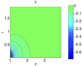
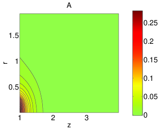
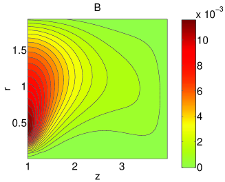
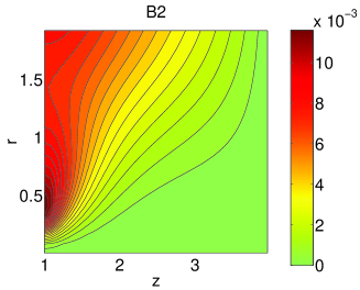
Figure 22: An illustration of $T,A,B$ and $B2$ for a star with $\xi=0.3$ and $\rho_{0}=5.0$. The star is dense enough that the configuration is non-linear, the peak value of $|T|$ being $\simeq 0.7$. As discussed earlier the metric contains singular terms involving $B$. Not only can we relax $B$ using the bulk equations, we can also integrate $B$ out from the origin $r=0$ using the constraint $\{rz\}$ to find another function, $B2$, which would equal $B$ if the Einstein equations were satisfied exactly. $B2$ has cleaner quadratic behavior at $r=0$ than the relaxed $B$, and is therefore used to calculate some of the singular source terms in the $B$ bulk ‘Poisson’ equation, rendering the source term more stable. The key point we see in the plot here is that the two values of $B$ and $B2$ agree very well over the lower half of the lattice, $r<0.5\,r_{\rm max}$. In the upper half of the lattice $B$ is forced to zero by the boundary conditions imposed whereas the integrated $B2$ is not. Even there, the difference between the functions is small compared to the values of the other metric functions $T,A$. It is only over the lower half of the lattice that the singular source terms have significant contribution (see figure 23) due to their suppression by $\frac{1}{r}$ factors, and therefore the plots suggest that the singular term approximation is very good. They also show that whilst $B$ and $B2$ differ at large $r$, the difference is very small in absolute terms showing the constraints are well satisfied. (lattice: $dr=0.01$, $r_{\rm max}=2$, $dz=0.01$, $z_{\rm max}=4$)

   

 

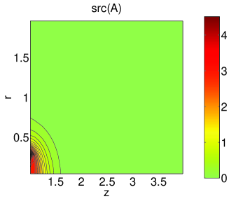
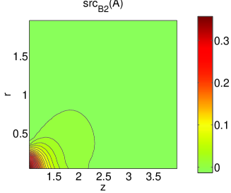
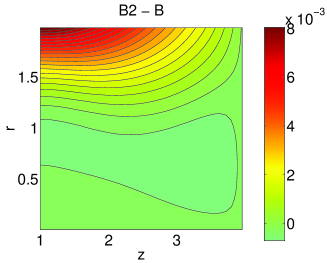
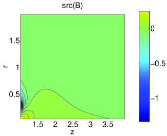
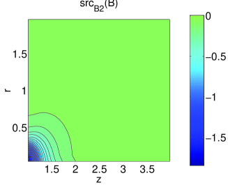
Figure 23: An illustration of $src(A),src_{B2}(A),src(B),src_{B2}(B)$ and $B2-B$ for the configuration $\xi=0.3$ and $\rho_{0}=5.0$ shown in figure 22. The top right frame shows the difference between $B$ and the integrated $B2$, used for the singular source terms in the $B$ equation, as integration out from the origin gives cleaner quadratic behavior at $r=0$. There is very good agreement between $B$ and $B2$, with $B2-B$ being very small, showing the constraints are well satisfied. The divergence at large $r$ is still very small in absolute terms (see figure 22). On the top left and bottom left are the plots $src(A),src(B)$ which show the full source terms for the $A$ and $B$ bulk ‘Poisson’ equations (15). On their right are $src_{B2}(A),src_{B2}(B)$ which are the contributions from the singular terms where $B$ is replaced by $B2$ to get improved regular behavior at $r=0$. We see that for $A$ these contributions are small compared to the other non-singular terms, but for $B$ they are significant. We also see that all the source terms are localized about the origin, exactly where we see $B2$ is an excellent approximation to $B$. This justifies the use of the method and also indicates why it works so effectively. Although integrating $B2$ is highly non-local, as the source terms are confined near the origin, the non-locality is not transfered into the relaxation procedure and we obtain a stable method.

7.2 Degree of Einstein Equation Violation

We graphically illustrate the constraints $\{rr-zz\}$ and $\{rz\}$ in figure 24, together with the errors in the equations (15) for $A,B$. The bulk equations for $T,A,B$ are relaxed to machine precision, but in the $A,B$ equations some singular terms in the source are calculated from $B2$ rather than $B$. Here we plot the error in these $A,B$ equations by differencing the left- and right-hand sides of the ‘Poisson’ equations (15), but using only $B$ to calculate the source. This difference then gives the error due to the singular term regularization scheme.

We firstly note that the errors in the $A$ source are much less than in $B$. This is evident from the previous section where we saw the contribution to the $A$ source from singular terms is correspondingly less. As expected, the errors are localized mainly about the origin. Now consider the constraint $\{rz\}$. This has no singular terms and has no large violations at the origin. The maximum values of violation occur at large $z$ and the error is small compared to that of $\{rr-zz\}$, which is localized at the origin and is $\sim 5$ times greater. We conclude from this that the constraints are indeed well satisfied, as indicated by $\{rz\}$, the major contribution to the error in the $\{rr-zz\}$ equation appearing not to come from asymptotic violations due to finite lattice size but rather from the singular term regularization.

We must compare these values to the physical curvatures of the solutions. The Weyl components provide just such a measure. In fact we compare with the quantities $C1,C2,C3,C4$ which have the blue-shifting factor of $\frac{1}{z^{2}}$ removed, discussed in appendix 8.1, as the $A,B$ equations and constraints similarly have this factor removed relative to the Einstein tensor components. The peak value of these quantities is $|C2|_{\rm peak}\simeq 14$. In addition, the peak curvatures are not located on the $r=0$ axis (eg. figure 26) and thus are not sensitive to the singular term regularization procedure there. It is not physically sensible to make a direct numerical comparison, but these physical curvatures are clearly much larger than the errors induced from the origin regularization scheme by a factor of $\sim 50$. Indeed, comparing to the constraint $\{rz\}$ which we saw above appears not to suffer directly from the origin singular terms, the factor is even larger $\sim 250$, indicating that the asymptotic boundary conditions and Bianchi identities are well satisfied. This is consistent with the conclusions of the comparison with the independent linear method of section 4, the linear method satisfying the asymptotic behavior, and constraints, and agreeing extremely well with the non-linear method in the low density regime. Furthermore, the close agreement of $B$ in the solutions of the linear and non-linear method confirms the origin regularization scheme performs well. This section shows the quality of solution remains high for non-linear configurations.

 

 

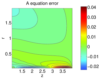
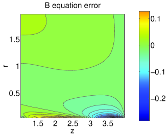
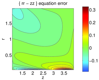
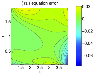
Figure 24: Plots of all the Einstein equations for $\xi=0.3$, with non-linear source $\rho_{0}=5.0$. Top; an illustration of error in the $A,B$ equations when using the true $B$ for the singular source terms rather than $B2$. Bottom; the constraints $\{rz\},\{rr-zz\}$. Note that the $T$ equation error is effectively zero as there are no singular source terms where $B$ is substituted for $B2$. As one would expect, the largest errors are found near $r=0$. It must be noted that the peak absolute value of the Weyl components $C1,C2,C3,C4$ is $\simeq 14$ and these peak values occur away from the symmetry axis and thus are not effected by the singular term regularization, (eg. see figure 26 for the components on the brane and symmetry axis for the slightly denser $\rho_{0}=7.0$ star). Thus the peak Einstein equation error is $\simeq 2\%$ of this peak physical curvature value, implying the Einstein equations, both elliptic and constraints are more than adequately satisfied at the resolution and lattice size used. (lattice: $dr=0.01$, $r_{\rm max}=2$, $dz=0.01$, $z_{\rm max}=4$)

7.3 Convergence and Finite Size Properties

The convergence of solutions with increasing $r$ and $z$ resolution was tested, figure 25 showing various intrinsic brane quantities for differing $dz$. Second order convergence is clearly seen, and also for varying $dr$ which is not plotted here. For $dr$ the resolution is relatively higher, the extrapolated continuum values for the metric functions on the brane differing from those at the resolutions used elsewhere in the paper, by a maximum of $\sim 0.3\%$, for $\xi=3.0$ stars. This is clearly much smaller than any systematic expected from section 4. The case of varying $dz$ is more interesting than $dr$ as there is a fundamental bound on resolution from the coordinate distance of the brane to the boundary of AdS, at $z=0$. For small stars the total lattice size may be a few AdS lengths and the brane is positioned at $z=1$. Thus even at low resolutions the lattice does ‘see’ that the brane is not located at the very singular boundary. Similarly in $r$, where the lattice is chosen to be a factor of $\sim 10$ wider than the star itself, and only on extremely coarse lattices would the star fail to be resolved. Whilst the situation in $r$ remains the same for large stars, such as $\xi=3$, the $z$ lattice extends out to $z\sim 45$, and the distance between the boundary and $z=1$ must still be well resolved or the solution will behave in a singular manner at the brane, and not relax. Thus large $z$ resolutions are critical in order to get convergence for large stars. Whilst the $r$ resolution can scale with the star radius, the $z$ resolution must be $dz\lesssim 0.1$ regardless of the star radius or the solutions will not relax. For the largest stars computed, the typical resolution used, $dz=0.03$, gives a maximum difference of $\simeq 10\%$ from the extrapolated continuum value for the metric functions. This is of order the differences with the independent linear method of section 4, expected to give a measure of systematic error. Thus in section 5.4 we extrapolate to a continuum value using two different $dz$ lattices to calculate the same solution. The details of the procedure are described in appendix 8.3. It is not exact, as with less resolution the solutions for denser stars do not converge, and thus the extrapolation must itself be extrapolated. However the error in this is expected to be much less than the systematic indicated in section 4.

It is crucial to test the sensitivity of the solutions to the physical size of the lattice. Table 1 shows averages of the absolute values of both the constraints, and in addition the equation $\{rr+zz\}$ for various lattice sizes. As discussed, $\{rr+zz\}$ is an elliptic equation which is satisfied to machine precision, but with the singular term approximation. The $\{rr+zz\}$ given here is without this singular term replacement and therefore indicates the error involved in this approximation. The averages in the tables are computed over the common inner region of the lattices, excluding the innermost 5 grid points which, whilst being well behaved and regular even with the $\frac{1}{r}$ terms in the constraints, would weight the regularization errors near the axis very strongly.

We find that varying the size of the lattice in the $r$ direction keeping $z_{\rm max}$ fixed has little effect on the constraints. Thus the size changes displayed only involve the $z$ extent, which for our configurations and resolutions does influence the quality of the solution. One clearly sees that increasing $z_{\rm max}$, keeping the $z$ resolution and $r_{\rm max}$ fixed, decreases both the constraints and also $\{rr+zz\}$. One sees that for the larger star, $\xi=1$, the effect is very dramatic if $z_{max}<r_{max}$. Empirically we find that the lattice must be as large or larger in $z$ than in $r$ to get good quality solutions, the effect being more marked the larger the star. In terms of absolute constraint violation we may compare these averaged values to the physical curvature computed in the rescaled Weyl tensor components $C1,C2,C3,C4$ (appendix 8.1) and again we see that both the constraint violation, and the error due to the singular source term regularization using $B2$, are again several orders of magnitude smaller than the curvatures generated in these solutions. We see the averaged error $<|\{rr+zz\}|>$ also becomes less, together with the constraints. This is because $B2$ is integrated, using the $\{rz\}$ constraint, in from $r=0$ and the $z_{max}$ boundary. The better the boundary conditions at $z_{\rm max}$, the closer $B$ is to $B2$ globally and the better the approximation.

 

 

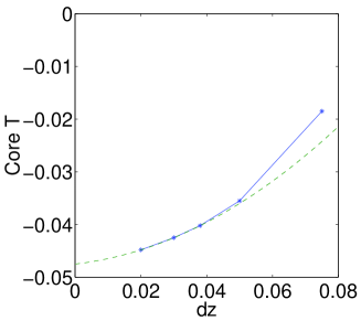
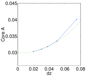
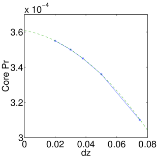
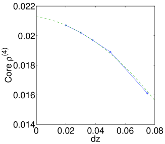
Figure 25: An illustration of convergence tests for the largest star with $\xi=3.0$ and a low density $\rho_{0}=0.02$. The lattice $z$ resolution is varied whilst keeping $z_{\rm max}$ fixed. Note that $r$ resolution variation behaves in a similar manner giving second order convergent quantities. The $z$ resolution is more interesting in its behavior as the brane has a coordinate distance of one unit from $z=0$. Thus in order to capture behavior well one requires much better resolution, $dz<<1$. The core values ($r=0,z=1$) for the metric functions $T,A$ and the core pressure and effective density are plotted against varying $dz$. Second order behavior is seen in $dz$ as expected and quadratic fits are performed (shown as the dotted line) using the smallest 3 values of $dz$, the extrema of the quadratic fits each being consistent with $dz=0$, as required by second order scaling. We see a deviation from the quadratic fit at large $dz$. The largest variation is seen in $T$ and for $dz=0.075$ the value is over a factor of two different from its apparent continuum value. In both $T,A$ the largest point appears to deviate from the quadratic scaling. For $dz=0.15$ no convergence was possible, the method behaving unstably. When $dz$ is much larger than $\sim 0.1$ the scaling deviates from its asymptotic form as the lattice no longer resolves the gap between the brane and singular boundary $z=0$. In fact comparing the $dz=0.03$ values with the continuum extrapolation we find the largest error for $T$ gives a $\sim 10\%$ variation, the other quantities having smaller errors $\lesssim 4\%$. $dz=0.03$ is the resolution used elsewhere in this paper for large star calculations. (lattice: $dr=0.2$, $r_{\rm max}=20$, $dz={\rm various}$, $z_{\rm max}=46$)

$\rho_{0}$	$\xi$	$r_{\rm max}$	$z_{\rm max}$	$<|\{rz\}|>$	$<|\{rr-zz\}|>$	$<|\{rr+zz\}|>$	$|C2|_{peak}$
0.1	0.3	2.0	1.5	3.2$\times 10^{-4}$	1.5$\times 10^{-3}$	2.0$\times 10^{-3}$	0.32
(linear)	(small)		2.0	1.0$\times 10^{-4}$	0.79$\times 10^{-3}$	1.1$\times 10^{-3}$
			3.0	0.30$\times 10^{-4}$	0.31$\times 10^{-3}$	0.38$\times 10^{-3}$
5.0	0.3	2.0	1.5	2.7$\times 10^{-2}$	1.3$\times 10^{-1}$	1.7$\times 10^{-1}$	14.1
(non-linear)	(small)		2.0	0.83$\times 10^{-2}$	0.62$\times 10^{-2}$	0.89$\times 10^{-1}$
			3.0	0.24$\times 10^{-2}$	0.24$\times 10^{-2}$	0.29$\times 10^{-1}$
0.01	1.	10.	6.0	6.1$\times 10^{-5}$	2.3$\times 10^{-4}$	1.6$\times 10^{-4}$	1.1$\times 10^{-2}$
(linear)	(medium)		10.	0.93$\times 10^{-5}$	0.27$\times 10^{-4}$	0.30$\times 10^{-4}$
			15.	0.29$\times 10^{-5}$	0.12$\times 10^{-4}$	0.12$\times 10^{-4}$

Table 1: Table showing constraint violation for 3 configurations; two sizes, $\xi=0.3,1$, and both linear and non-linear densities for one size, $\rho_{0}=0.1,5.0$ respectively for $\xi=0.3$. One finds that for $r$ resolutions high enough to capture the density profile accurately, increasing or decreasing the lattice size makes little difference to the constraints. It is the extent of the lattice in the $z$ direction that determines the constraint satisfaction. The absolute values of the constraints are averaged over lattices with different $z_{\rm max}$. The average is taken only over the common portion of the lattices for a given $\xi,\rho_{0}$. The first 5 lattice points in $r$ are excluded as $\frac{1}{r}$ contributions receive an unphysically large weighting there. In all cases the constraints are better satisfied as $z_{\rm max}$ is increased for fixed $z$ resolution. The effect is more marked for the larger star with $\xi=1$. This is because the metric falls away less quickly in $z$ the larger the star, and thus the lattice must be large enough in $z$ to ensure asymptotic AdS is well approximated. Typically for $z_{\rm max}\gtrsim r_{\rm max}\gtrsim 6\xi$ the lattice is large enough to accommodate the star. We see in the $\xi=1$ case that there is a huge improvement in increasing $z_{\rm max}$ from $0.5\,r_{\rm max}$ to $r_{\rm max}$, but then the improvement is much less for the next increase to $1.5\,r_{\rm max}$, showing that the perturbation was not captured for $z_{\rm max}=0.5\,r_{\rm max}$, but is for $z_{\rm max}\geq r_{\rm max}$. Note that the peak value of the Weyl component $C2$ (see appendix 8.1) is shown. This allows one to compare the average constraint violation against a quantity which characterizes the curvature. We see that the average constraint violations are considerably smaller, $\sim 1000$ times, for the two linear configurations and for the non-linear one even more. Thus the constraints appear to be even better satisfied relative to the perturbation for dense stars, the regime of interest for this paper. The elliptic equation $\{rr+zz\}$ is also plotted, but now without the singular source terms replaced using the integrated $B2$ solution. Of course with the $B2$ replacement this equation is satisfied to very high precision as specified by the relaxation procedure. Without the replacement, the quality of the approximation can be assessed. Note that the violation of this equation has similar behavior with grid size to that of $\{rz\}$. This is to be expected as $B2$ is integrated using the $\{rz\}$ constraint equation. Therefore when this equation is better satisfied, the $B2$ source term replacement is also a better approximation. (For $\xi=0.3$; $dr=0.01$, $dz=0.01$. For $\xi=1$; $dr=0.1$, $dz=0.01$)

In table 2 we plot the core metric function values against lattice size in $z$. Again we see convergence of the solution as the physical $z$ size increases, although the variations in the values are much smaller, a maximum variation of $\sim 4\%$ over the range, compared with the averaged constraints of table 1 which vary by an order of magnitude over the range. Similarly calculating the observables on the brane, outlined in section 5.1, the density and pressures, both actual and induced, and in addition the induced Weyl component, all give the same small variations over the range of lattice sizes, as they are constructed from these metric functions. Thus we find that the brane geometry, our primary interest, is not sensitive to the lattice size, and thus the exact form of the horizon metric, although the constraints are.

$\rho_{0}$	$\xi$	$r_{\rm max}$	$z_{\rm max}$	$T_{0}$	$A_{0}$
0.1	0.3	2.0	1.5	-0.007500	0.004190
(linear)	(small)		2.0	-0.007512	0.004154
			3.0	-0.007513	0.004137
5.0	0.3	2.0	1.5	-0.7030	0.3047
(non-linear)	(small)		2.0	-0.6969	0.2989
			3.0	-0.6942	0.2965
0.01	1.	10.	6.0	-0.003698	0.002328
(linear)	(medium)		10.	-0.003692	0.002240
			15.	-0.003691	0.002237

Table 2: Table showing the variation of metric functions at the star core for the different size lattices used in table 1. We see that for the resolution used the core values of the metric functions, and indeed their profiles (not shown here), are very stable to changing the physical lattice size. This shows that the boundary conditions on the asymptotic $z$ boundary are accurately forcing the metric to AdS. The largest variation is found for the $\xi=1$ configuration, going from $z_{\rm max}$ being only $5$ to $10$. Although this has a large effect on the constraints which show a 6 fold decrease, the maximum change for the metric functions is in $A$ which varies by $4\%$. Note that the metric functions vary most at the core of the star as this is furthest from a boundary where they are fixed.

7.4 Asymptotic Behavior

We see that the asymptotic behavior is correct by examining the Weyl components. Whilst the metric functions may have a non-zero perturbation, some component of this may well be gauge. The Weyl components are non-zero only for physical curvatures. Figure 26 firstly shows that the 4 Weyl components decay quickly on the brane as $r$ approaches the asymptotic boundary, for both a typical small and large star solution. It also shows a magnified version of these components in the asymptotic $z$ regions of the same solution for fixed $r$ near the axis. This confirms that the curvature is dying away and asymptotic AdS is being approached at large $z$, implying the boundary conditions are as required. It is important to note that $C1,C2,C3,C4$ are not the Weyl components but rather have been scaled by $\frac{1}{z^{2}}$ to make them a better numerical estimator of the solution accuracy. Note that the fall off in $C1,C2,C3,C4$ for both the small and large stars shown in figure 26 is faster than $\frac{1}{z^{2}}$ for large $z$, which they are plotted against, implying the Weyl components, and therefore curvature invariants, do indeed go to zero. We see small boundary effects for the large star which imply that the actual Weyl components are very large at this boundary due to the $z^{2}$ factor, which is $\sim 10^{3}$ there. The advantage of plotting the rescaled $C1,C2,C3,C4$ against $\frac{1}{z^{2}}$ is that this is clearly seen to be a numerical artifact of the boundary, and the correct asymptotic AdS behavior is observed. Thus for both the asymptotic $r$ and $z$ boundaries the solutions are seen to correctly approach AdS.

 

 

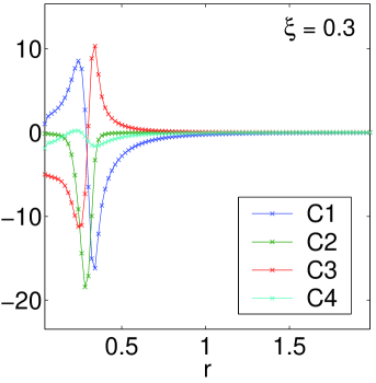
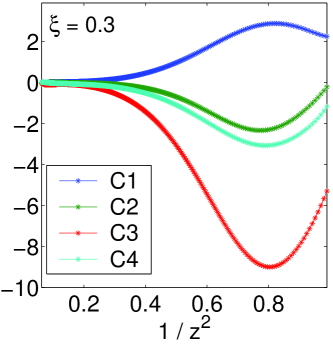
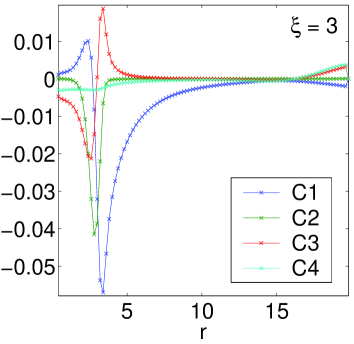
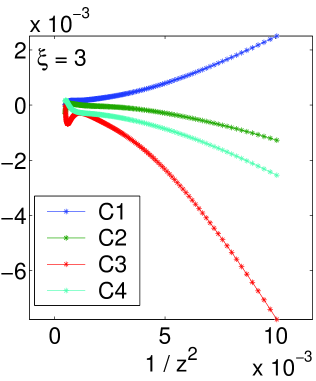
Figure 26: An illustration of $C1,C2,C3,C4$ for the densest small and large configurations used, top, $\xi=0.3$ with source $\rho_{0}=7.0$ and bottom, $\xi=3$ with $\rho_{0}=0.149$. On the left the plots show the components on the brane at $z=1$. Here $C1,C2,C3,C4$ give physical curvatures. Curvature invariants would be combinations of these quantities with no further $r,z$ dependence. These curvatures all decay to zero for large $r$. This occurs very cleanly for the small star, and slightly less cleanly for the large star with small curvature being induced at the edge of the lattice by the lattice boundaries. This is still only a maximum $5\%$ error compared to the peak curvatures. We conclude that the boundary condition $T,A,B\rightarrow 0$ as $r\rightarrow r_{\rm max}$ is therefore correctly reproducing the AdS behavior. We expect the finite boundaries to give some error for the larger stars as the correlation functions decay as $\frac{1}{r}$ rather than $\frac{1}{r^{2}}$ as for small stars, and so the perturbation decays more slowly. On the right are plots showing how the components $C1,C2,C3,C4$ decay towards the horizon for a fixed value of $r$ near the axis (for $\xi=0.3$, $r=0.1$ and $\xi=3.0$, $r=1.0$). As discussed in the appendix 8.1, these functions have the blue-shifting factor $\frac{1}{z^{2}}$ removed so that errors appropriate to the numerical solution can be seen. For the true curvature invariants to tend to zero, $C1,C2,C3,C4$ must decay faster than $\frac{1}{z^{2}}$, and therefore the functions are plotted against $\frac{1}{z^{2}}$. For both the small and large star it is clear that the functions do decay faster, the functions being shallower than linear as $\frac{1}{z^{2}}\rightarrow 0$. This implies that $T,A,B\rightarrow 0$ on the large $z$ boundary is reproducing asymptotic AdS. We also note that for the large star there are small errors at the boundary. If we had plotted the Weyl components with blue-shifting $z^{2}$ factor included, these points at $z\sim 40$ would completely dominate the plot, but we see here that they are simply small numerical errors confirming that the rescaled $C1,C2,C3,C4$ are the correct measures to use. ($\xi=0.3$ lattice: $dr=0.02$, $r_{\rm max}=2$, $dz=0.005$, $z_{\rm max}=4$; $\xi=3$ lattice: $dr=0.2$, $r_{\rm max}=20$, $dz=0.03$, $z_{\rm max}=46$)

8 Appendix B: Technical Details

8.1 Einstein Equations and Matching Conditions

In this appendix we give the Einstein tensor components, the matching equations and the Weyl tensor components for the metric (14). Expressing the metric in its natural one form basis,

$$ds^{2}=-w_{(t)}^{\mu}w_{(t)\mu}+w_{(r)}^{\mu}w_{(r)\mu}+w_{(\Omega)_{i}}^{\mu}w_{(\Omega)_{i}\mu}+w_{(z)}^{\mu}w_{(z)\mu}$$ (36)

where $i=\theta,\phi$, giving the one forms on an $S^{2}$. Firstly, the non zero Einstein tensor components are,

$$-w^{\mu}_{(t)}w^{\nu}_{(t)}G_{\mu\nu}=G^{t}_{~{}t}= z^{2}\,e^{-2\,(A+B)}\Big{[}\,\left[3\,\partial_{r}^{2}A-\partial_{r}^{2}B+3\,{({\partial_{r}A})^{2}}+3\,{({\partial_{r}B})^{2}}-6\,{({\partial_{r}A})\,({\partial_{r}B})}\right]+\left[\,\partial_{r}\leftrightarrow\partial_{z}\,\right]$$

$$\qquad+\frac{6}{r}\partial_{r}(A-B)-\frac{1}{r^{2}}\left(e^{4B}-1\right)-\frac{6}{z}\,\partial_{z}(A-B)+{\frac{6}{{z^{2}}}}\Big{]}$$

$$w^{\mu}_{(r)}w^{\nu}_{(z)}G_{\mu\nu}=G^{r}_{~{}z}= z^{2}\,e^{-2\,(A+B)}\Big{[}-2\,\partial_{r}\partial_{z}A+2\,\partial_{r}\partial_{z}B-\partial_{r}\partial_{z}T+2\,(\partial_{r}A)\,(\partial_{z}A)+2\,(\partial_{r}A)\,(\partial_{z}B)$$

$$\qquad+2\,(\partial_{r}B)\,(\partial_{z}A)-6\,(\partial_{r}B)\,(\partial_{z}B)+(\partial_{z}A)\,(\partial_{r}T)+(\partial_{z}B)\,(\partial_{r}T)+(\partial_{r}A)\,(\partial_{z}T)$$

$$\qquad+(\partial_{r}B)\,(\partial_{z}T)-(\partial_{r}T)\,(\partial_{z}T)+\frac{4}{r}\,\partial_{z}B-\frac{3}{z}\,r\,\partial_{r}(A+B)\Big{]}$$

$$w^{\mu}_{(r)}w^{\nu}_{(r)}G_{\mu\nu}=G^{r}_{~{}r}= z^{2}\,e^{-2\,(A+B)}\Big{[}+\partial_{z}^{2}T+2\,\partial_{z}^{2}A-2\,\partial_{z}^{2}B-2\,(\partial_{r}A)\,(\partial_{r}B)-6\,(\partial_{z}A)\,(\partial_{z}B)+3\,{({\partial_{r}A})^{2}}$$

$$\qquad-{({\partial_{r}B})^{2}}+{({\partial_{z}A})^{2}}+5\,{({\partial_{z}B})^{2}}+3\,(\partial_{r}A)\,(\partial_{r}T)-(\partial_{r}B)\,(\partial_{r}T)+(\partial_{z}A)\,(\partial_{z}T)$$

$$\qquad-3\,(\partial_{z}B)\,(\partial_{z}T)+{({\partial_{z}T})^{2}}+\frac{1}{r}\left(4\,\partial_{r}A+2\,\partial_{r}T\right)-\frac{1}{r^{2}}\left(e^{4B}-1\right)$$

$$\qquad+\frac{1}{z}\left(-3\,\partial_{z}A+9\,\partial_{z}B-3\,\partial_{z}T\right)+{\frac{6}{{z^{2}}}}\Big{]}$$

$$w^{\mu}_{(\Omega_{\theta})}w^{\nu}_{(\Omega_{\theta})}G_{\mu\nu}=G^{\theta}_{~{}\theta}= z^{2}\,e^{-2\,(A+B)}\Big{[}\,\left[\,2\partial_{r}^{2}A+{({\partial_{r}A})^{2}}+{({\partial_{r}B})^{2}}-2{({\partial_{r}A})\,({\partial_{r}B})}\right.$$

$$\qquad\left.+(\partial_{r}A)\,(\partial_{r}T)-(\partial_{r}B)\,(\partial_{r}T)+{({\partial_{r}T})^{2}}+\partial_{r}^{2}T\right]+\left[\,\partial_{r}\leftrightarrow\partial_{z}\,\right]$$

$$\qquad+\frac{1}{r}\left(+2\,\partial_{r}A-2\,\partial_{r}B+\partial_{r}T\right)+\frac{1}{z}\left(-3\,\partial_{z}A+3\,\partial_{z}B-3\,\partial_{z}T\right)+{\frac{6}{{z^{2}}}}\Big{]}$$

$$w^{\mu}_{(z)}w^{\nu}_{(z)}G_{\mu\nu}=G^{z}_{~{}z}= z^{2}\,e^{-2\,(A+B)}\Big{[}2\,\partial_{r}^{2}A-2\,\partial_{r}^{2}B+\partial_{r}^{2}T-6\,(\partial_{r}A)\,(\partial_{r}B)-2\,(\partial_{z}A)\,(\partial_{z}B)+{({\partial_{r}A})^{2}}$$

$$\qquad+5\,{({\partial_{r}B})^{2}}+3\,{({\partial_{z}A})^{2}}-{({\partial_{z}B})^{2}}+(\partial_{r}A)\,(\partial_{r}T)-3\,(\partial_{r}B)\,(\partial_{r}T)$$

$$\qquad+3\,(\partial_{z}A)\,(\partial_{z}T)-(\partial_{z}B)\,(\partial_{z}T)+{({\partial_{r}T})^{2}}+\frac{1}{r}\left(4\,\partial_{r}A-8\,\partial_{r}B+2\,\partial_{r}T\right)$$

$$\qquad-\frac{1}{r^{2}}\left(e^{4B}-1\right)+\frac{1}{z}\left(-9\,\partial_{z}A+3\,\partial_{z}B-3\,\partial_{z}T\right)+{\frac{6}{{z^{2}}}}\Big{]}$$ (37)

where in our units the Einstein equations are $G^{t}_{~{}t}=G^{r}_{~{}r}+G^{z}_{~{}z}=G^{\theta}_{~{}\theta}=6$ together with the constraint equations $G^{r}_{~{}z}=0$ and $G^{r}_{~{}r}-G^{z}_{~{}z}=0$. The matching equation (7) has non trivial components,

$$-6+6\,z\,\partial_{z}A-2\,z\,\partial_{z}B+\left(6+\rho\right)\,e^{A+B} =0$$

$$-6+4\,z\,\partial_{z}A-4\,z\,\partial_{z}B+2\,z\,\partial_{z}T+\left(6-P_{r}\right)\,e^{A+B} =0$$

$$-6+4\,z\,\partial_{z}A+2\,z\,\partial_{z}T+\left(6-P_{\theta}\right)\,e^{A+B} =0$$ (38)

with $P_{r},P_{\theta}$ being the radial and angular pressure components. Isotropy on the brane requires that these be equal and the last two component equations therefore imply that $B_{,z}=0$.

Together with the Einstein tensor, the Weyl tensor specifies the geometry. Given the symmetries of the metric, and of the Weyl tensor itself, it has 4 independent components, which can be taken as the following,

$$z^{2}C1 =w_{(t)}^{\mu}w_{(r)}^{\nu}w_{(t)}^{\alpha}w_{(r)}^{\beta}C_{\mu\nu\alpha\beta}=-C_{tr}^{~{}~{}~{}tr}$$

$$=z^{2}e^{-2(A+B)}\Big{[}-\frac{1}{2}\partial_{r}\partial_{r}A+\frac{1}{6}\partial_{r}^{2}B+\frac{1}{2}\partial_{r}^{2}T+\frac{1}{2}{({\partial_{r}A})^{2}}+\frac{1}{3}(\partial_{r}A)\,(\partial_{r}B)-\frac{5}{6}\,{({\partial_{r}B})^{2}}$$

$$\qquad\qquad-(\partial_{r}A)\,(\partial_{r}T)-\frac{1}{3}(\partial_{r}B)\,(\partial_{r}T)+\frac{1}{2}{({\partial_{r}T})^{2}}+\frac{1}{6}\partial_{z}^{2}A-\frac{1}{2}\partial_{z}^{2}B$$

$$\qquad\qquad-\frac{1}{6}\partial_{z}^{2}T-\frac{1}{6}{({\partial_{z}A})^{2}}-(\partial_{z}A)\,(\partial_{z}B)+\frac{7}{6}\,{({\partial_{z}B})^{2}}+\frac{1}{3}(\partial_{z}A)\,(\partial_{z}T)+(\partial_{z}B)\,(\partial_{z}T)$$

$$\qquad\qquad-\frac{1}{6}{({\partial_{z}T})^{2}}+\frac{1}{r}\left(+{\frac{\partial_{r}A}{3\,r}}+{\frac{\partial_{r}B}{r}}-{\frac{\partial_{r}T}{3\,r}}\right)-\frac{1}{6r^{2}}\left(e^{4\,B}-1\right)\Big{]}$$

$$z^{2}C2 =w_{(t)}^{\mu}w_{(r)}^{\nu}w_{(t)}^{\alpha}w_{(z)}^{\beta}C_{\mu\nu\alpha\beta}=-C_{tr}^{~{}~{}~{}tz}$$

$$=z^{2}e^{-2(A+B)}\Big{[}-\frac{2}{3}\,\partial_{r}\partial_{z}A+\frac{2}{3}\,\partial_{r}A\,\partial_{z}A+\frac{2}{3}\,\partial_{z}A\,\partial_{r}B+\frac{2}{3}\,\partial_{r}\partial_{z}B+\frac{2}{3}\,\partial_{r}A\,\partial_{z}B-2\,\partial_{r}B\,\partial_{z}B$$

$$\qquad\qquad-\frac{2}{3}\,(\partial_{z}A)\,(\partial_{r}T)-\frac{2}{3}\,(\partial_{z}B)\,(\partial_{r}T)+\frac{2}{3}\,\partial_{r}\partial_{z}T-\frac{2}{3}\,(\partial_{r}A)\,(\partial_{z}T)$$

$$\qquad\qquad-\frac{2}{3}\,(\partial_{r}B)\,(\partial_{z}T)+\frac{2}{3}\,(\partial_{r}T)\,(\partial_{z}T)+\frac{4}{3\,r}\,\partial_{z}B\Big{]}$$

$$z^{2}C3 =w_{(t)}^{\mu}w_{(z)}^{\nu}w_{(t)}^{\alpha}w_{(z)}^{\beta}C_{\mu\nu\alpha\beta}=-C_{tz}^{~{}~{}~{}tz}$$

$$=z^{2}e^{-2(A+B)}\Big{[}+\frac{1}{6}\partial_{r}^{2}A-\frac{1}{2}\partial_{z}^{2}A-\frac{1}{2}\partial_{r}^{2}B+\frac{1}{6}\partial_{z}^{2}B-\frac{1}{6}\partial_{r}^{2}T+\frac{1}{2}\partial_{z}^{2}T-\frac{1}{6}{({\partial_{r}A})^{2}}-(\partial_{r}A)\,(\partial_{r}B)$$

$$\qquad\qquad+\frac{7}{6}\,{({\partial_{r}B})^{2}}+\frac{1}{3}(\partial_{r}A)\,(\partial_{r}T)+(\partial_{r}B)\,(\partial_{r}T)-\frac{1}{6}{({\partial_{r}T})^{2}}+\frac{1}{2}{({\partial_{z}A})^{2}}$$

$$\qquad\qquad+\frac{1}{3}(\partial_{z}A)\,(\partial_{z}B)-\frac{5}{6}\,{({\partial_{z}B})^{2}}-(\partial_{z}A)\,(\partial_{z}T)-\frac{1}{3}(\partial_{z}B)\,(\partial_{z}T)+\frac{1}{2}{({\partial_{z}T})^{2}}$$

$$\qquad\qquad+\frac{1}{r}\left(+\frac{1}{3}\partial_{r}A-\frac{5}{3}\,\partial_{r}B-\frac{1}{3}\partial_{r}T\right)-\frac{1}{6\,r^{2}}\left(e^{4\,B}-1\right)\Big{]}$$

$$z^{2}C4 =w_{(r)}^{\mu}w_{(z)}^{\nu}w_{(r)}^{\alpha}w_{(z)}^{\beta}C_{\mu\nu\alpha\beta}=C_{rz}^{~{}~{}~{}rz}$$

$$=z^{2}e^{-2(A+B)}\Big{[}-\frac{1}{6}\partial_{r}^{2}A-\frac{1}{6}\partial_{z}^{2}A-\frac{5}{6}\,\partial_{r}^{2}B-\frac{5}{6}\,\partial_{z}^{2}B+\frac{1}{6}\partial_{r}^{2}T+\frac{1}{6}\partial_{z}^{2}T+\frac{1}{6}{({\partial_{r}A})^{2}}-\frac{1}{3}(\partial_{r}A)\,(\partial_{r}B)$$

$$\qquad\qquad+\frac{1}{6}{({\partial_{r}B})^{2}}-\frac{1}{3}(\partial_{r}A)\,(\partial_{r}T)+\frac{1}{3}(\partial_{r}B)\,(\partial_{r}T)+\frac{1}{6}{({\partial_{r}T})^{2}}+\frac{1}{6}{({\partial_{z}A})^{2}}$$

$$\qquad\qquad-\frac{1}{3}(\partial_{z}A)\,(\partial_{z}B)+\frac{1}{6}{({\partial_{z}B})^{2}}-\frac{1}{3}(\partial_{z}A)\,(\partial_{z}T)+\frac{1}{3}(\partial_{z}B)\,(\partial_{z}T)+\frac{1}{6}{({\partial_{z}T})^{2}}$$

$$\qquad\qquad+\frac{1}{r}\left(+\frac{1}{3}\partial_{r}A-\frac{1}{3}\partial_{r}B-\frac{1}{3}\partial_{r}T\right)+\frac{1}{6\,r^{2}}\left(e^{4\,B}-1\right)\Big{]}$$ (39)

Note that in both the Einstein and Weyl tensor components above, the indices are arranged as they appear in curvature invariants, an overall blue-shifting factor of $z^{2}$ appearing. This blue-shifting factor will amplify numerical errors on the lattice. We therefore define the rescaled Weyl tensor quantities $C1,C2,C3,C4$ above, and Einstein equations $\{AB\}$,

$$\{AB\}=\frac{1}{z^{2}}w_{(A)}^{\mu}w_{(B)}^{\nu}(G_{\mu\nu}-6g_{\mu\nu})$$ (40)

which have the factor removed. The elliptic equations and constraints, solved by relaxation and integration, have no such factor as it simply multiplies the whole Einstein tensor components homogeneously. Thus we shall use these rescaled quantities to assess the numerical errors, the terms now having no $z$ prefactor, as for the equations that are numerically solved. Using the original scaling would blow up tiny errors at large $z$, and as we expect there to be such errors from finite boundary effects this is less than satisfactory. For small stars this is no problem, but we find for the large stars that there do exist small boundary errors, which are hugely amplified when multiplied by $z^{2}$ which may be $\sim 10^{3}$. We check that the metric solutions are insensitive to these boundary conditions (appendix 7), and finding that they are, must conclude that the geometric quantities are not a good measure of solution quality as tiny changes in the metric at large $z$ give huge changes in the Weyl components due to the blue-shifting. The quantities that reside on the brane at $z=1$ are totally unaffected.

We conclude the section by giving the 3 independent components of the 4-dimensional Einstein tensor, and the 1 independent component of the 4-dimensional Weyl tensor, for the induced metric (33). These are,

$$\rho^{(4)}=G^{(4)t}_{~{}~{}~{}~{}t} =e^{-2(A+B)}\Big{[}2\partial^{2}_{r}B-2\partial^{2}_{r}A-5(\partial_{r}B)^{2}-(\partial_{r}A)^{2}+6\partial_{r}A\partial_{r}B$$

$$\qquad\qquad+\frac{1}{r}\left(8\partial_{r}B-4\partial_{r}A\right)+\frac{1}{r^{2}}\left(e^{4B}-1\right)\Big{]}$$

$$P_{r}^{(4)}=G^{(4)r}_{~{}~{}~{}~{}r} =e^{-2(A+B)}\Big{[}-2(\partial_{r}T)(\partial_{r}B)-2(\partial_{r}A)(\partial_{r}B)+2(\partial_{r}A)(\partial_{r}T)+(\partial_{r}A)^{2}+(\partial_{r}B)^{2}$$

$$\qquad\qquad+\frac{2}{r}\left(\partial_{r}T+\partial_{r}A-\partial_{r}B\right)-\frac{1}{r^{2}}\left(e^{4B}-1\right)\Big{]}$$

$$P_{\theta}^{(4)}=G^{(4)\theta}_{~{}~{}~{}~{}\theta} =e^{-2(A+B)}\Big{[}\partial^{2}_{r}T+\partial^{2}_{r}A-\partial^{2}_{r}B+2(\partial_{r}B)^{2}+(\partial_{r}T)^{2}-2(\partial_{r}T)(\partial_{r}B)-2(\partial_{r}A)(\partial_{r}B)$$

$$\qquad\qquad+\frac{1}{r}\left(\partial_{r}A+\partial_{r}T-3\partial_{r}B\right)\Big{]}$$ (41)

and the Weyl component,

$$C^{(4)}=C_{tr}^{~{}~{}~{}tr} =-\frac{1}{3}e^{-2(A+B)}\Big{[}+\partial^{2}_{r}T-\partial^{2}_{r}A+\partial^{2}_{r}B-2(\partial_{r}A)(\partial_{r}T)+(\partial_{r}T)^{2}+(\partial_{r}A)^{2}-(\partial_{r}B)^{2}$$

$$\qquad\qquad+\frac{1}{r}\left(\partial_{r}B+\partial_{r}A-\partial_{r}T\right)+\frac{1}{r^{2}}\left(1-e^{4B}\right)\Big{]}$$ (42)

8.2 Asymptotic Linear Behavior

One can solve the linear theory for a point source. The $a$ equation (24) solution is constructed from the modes satisfying the radiation boundary conditions, discussed in section 1.2, as,

$$a(r,z)=\sqrt{\frac{2}{\pi}}\int_{0}^{\infty}dp\,a(p)\,(pr)^{-\frac{3}{2}}\,J_{\frac{3}{2}}(pr)\,(pz)^{2}\,K_{2}(pz)$$ (43)

for some coefficients $a(p)$. Let us consider $a(p)=a_{0}$. Then,

$$a(r,z)=\frac{a_{0}}{\sqrt{r^{2}+z^{2}}}$$ (44)

and we can solve (25) and (26), and find,

$$g(r,z) =a_{0}\frac{z}{\sqrt{r^{2}+z^{2}}}+\int_{0}^{\infty}dpF(p)\cos{pr}\,e^{-pz}$$

$$f(r,z) =-a_{0}\frac{r}{\sqrt{r^{2}+z^{2}}}-\int_{0}^{\infty}dpF(p)\sin{pr}\,e^{-pz}$$ (45)

and imposing the matching condition, $\partial_{z}a=-\frac{2}{r}\partial_{r}g$ at $z=1$, from (28), we obtain

$$F(p)=-\frac{3a_{0}}{\pi}K_{0}(p)e^{p}$$ (46)

On the brane we calculate,

$$g =-\frac{a_{0}}{2\sqrt{1+r^{2}}}\sim-\frac{a_{0}}{2}\frac{1}{r}+O(\frac{a_{0}}{r^{3}})$$

$$f =-\frac{a_{0}}{\sqrt{1+r^{2}}}(r-\frac{3}{\pi}\sinh^{-1}{r})\sim-a_{0}+\frac{3a_{0}}{\pi}\frac{\log{2r}}{r}+O(\frac{a_{0}}{r^{2}})$$ (47)

Then, $g\sim-a_{0}/2r+O(1/r^{3})$ which to leading order in large $r>>1$ (ie. large compared to the AdS length) is the inverse $r$ response to a point density source on the brane at $r=0$ from equation (28). From (27), we see that at large $r$ on the brane, $T,A,B\rightarrow 0$.

At large $z>>1$ we receive contributions from modes with $k<<1$ and therefore expand $K_{0}(k)$, in large $z$ and large $r$ such that $r<<z$, to yield,

$$a =\frac{a_{0}}{z}(1+O(\frac{r^{2}}{z^{2}}))$$

$$f =a_{0}\frac{r}{z}(-1+\frac{3}{\pi}\frac{1}{z}(\log(2)-1+\log(z))+O(|\frac{\log{z}}{z^{2}}|+\frac{r^{2}}{z^{2}}))$$

$$g =a_{0}(1-\frac{3}{\pi}\frac{1}{z}(\log{2}+\log{z})+O(|\frac{\log{z}}{z^{2}}|+\frac{r^{2}}{z^{2}}))$$ (48)

implying, from (27), that,

$$T =a_{0}\frac{1}{z}(-4+O(|\frac{\log{z}}{z}|+\frac{r^{2}}{z^{2}}))$$

$$A =a_{0}\frac{1}{z}(-1+O(|\frac{\log{z}}{z}|+\frac{r^{2}}{z^{2}}))$$

$$B =a_{0}\frac{1}{z}\frac{r^{2}}{z^{2}}(\frac{3}{4}+O(\frac{r^{2}}{z^{2}}))$$ (49)

and therefore indeed $T,A,B\sim 1/z\rightarrow 0$ as $z\rightarrow\infty$. Note that this is a good approximation for $r>>1$ with $r<z$, and represents the asymptotic form for a point density source.

Examining the Weyl components of the previous appendix section, 8.1, we also see that these in fact decay as $\sim 1/z$ for large $z$. The way the functions $T,A$ enter is always with derivatives taken. Derivatives involving $r$ remove the leading $1/z,\log{z}/z$ terms, and the resulting $1/z^{3}$ behavior cancels the overall $z^{2}$ factor in these Weyl components, with indices arranged as they occur in curvature invariants, to yield $1/z$ asymptotically. Derivatives in $z$ simply reduce the leading $1/z$ to higher inverse powers which again combine with the overall $z^{2}$ to give $1/z$ asymptotically. There are more subtle terms in $B$, such as those involving no derivatives, $z^{2}(e^{4B}-1)/r^{2}$ or only one $z$ derivative, $z^{2}\partial_{z}B/r$. However, we note that $B$ in fact scales as $1/z^{3}$ unlike $T,A$ and thus these terms have the decaying behavior too. Thus, in the linear theory, asymptotically all the Weyl components do indeed decay and the horizon geometry is regular, and that of AdS.

8.3 Numerical Details: Finite Differencing, Relaxation and Integration Schemes

The lattice used to cover the $rz$ plane is rectangular, with even spacing $dr,dz$ in the $r,z$ directions. We discretize the fields over the lattice as $X_{i,j}$ where $i,j$ are the $r$ and $z$ positions respectively and run as $i=0,1,\ldots i_{\rm max}$, $j=0,1,\ldots j_{\rm max}$. The lattice is truncated at a maximum size in both $r$ and $z$ and the boundary conditions $T,A,B=0$ are applied there.

The elliptic equations are differenced using standard second order templates, and the second derivative terms imply they are naturally evaluated at $(i,j)$. The constraint equation $\{rz\}$ contains terms taking the generic form,

$$\partial_{r}\partial_{z}X+a\,\frac{1}{r}\partial_{r}Y+b\,\partial_{r}X\partial_{z}Y+\ldots=0$$ (50)

where $X,Y$ are some metric functions. This is then evaluated at the center of a lattice cell $(i+\frac{1}{2},j+\frac{1}{2})$, compatible with the second order mixed derivative operators. This equation is used to integrate $T$ along the brane boundary by evaluating it at $(i+\frac{1}{2},\frac{1}{2})$ solving it for $T_{i,0}$ which allows an integration in from $r=\infty$ iteratively if $T_{i+1,0}$ is known and the bulk values $T_{i,1},T_{i+1,1}$ are also known. Similarly the Einstein tensor components $G^{r}_{~{}r}$ and $G^{z}_{~{}z}$ reside naturally at $z=z_{i+\frac{1}{2},j}$ and $z=z_{i,j+\frac{1}{2}}$ respectively, as indicated by their highest derivative operators, the first having only first order $r$ derivatives and the second, only first order $z$ derivatives. The matching conditions are of generic form,

$$z\,\partial_{z}X+\rho e^{Y}=0$$ (51)

where again $X,Y$ schematically represent metric functions. The first order derivative operators imply the brane naturally resides midway between $j=0,1$ at $z=z_{i,\frac{1}{2}}$.

The elliptic equations are solved by splitting the Laplacian term from the source term in (15),

$$\nabla^{2}X={\rm Src}_{X}(T,A,B)$$ (52)

where ${\rm Src}_{X}$ are the source functionals and $X=T,A,B$. An over-relaxation scheme is used to partially relax the 3 Poisson equations holding the sources constant. The sources are then updated with the new values of $T,A,B$ calculated from the Poisson equations. At each step, only a few cycles of the over-relaxation are computed. This is iterated, and at each update step the boundary conditions are imposed. Relaxation is continued until machine precision is reached. More sophisticated Poisson solvers were implemented but the highly local behavior of the over-relaxation scheme appeared to give quicker and more reliable overall convergence.

The $\{rz\}$ constraint can be used to integrate $B$ out from the origin $r=0$, determining $B_{i+1,j}$ in terms of $B_{i,j},B_{i,j+1},B_{i+1,j+1}$. As discussed in section 3.6, this is used to calculate some of the source terms in ${\rm Src}_{A,B}$, the source functional for the $A$ and $B$ bulk equations. The terms we replace are the ones that have singular coefficients as $r\rightarrow 0$ in front of $B$, and its derivatives. There are no such terms in the $T$ equation. For the $A$ and $B$ equations we rewrite the sources as

$$\nabla^{2}A ={\rm Src}^{(2)}_{A}+\frac{\partial_{r}B2}{r}$$

$$\nabla^{2}B ={\rm Src}^{(2)}_{B}+-{\frac{3\,\partial_{r}B2}{r}}+\frac{1}{r^{2}}\left(1-e^{4\,B2}\right)$$ (53)

where $B2$ is the solution of $B$ calculated from integrating the $\{rz\}$ equation. The terms ${\rm Src}^{(2)}_{A,B}$ refer to the remainder of the source terms as in equations (15).

In section 7 the magnitude of the $B2$ source terms, compared to the other non-singular source terms, are calculated for a typical solution. These sources are suppressed by inverse powers of $r$ so that they contribute locally near the axis, and not asymptotically at large $r$. Thus although the integration for $B2$ is non-local over the lattice, the sources it generates for the bulk equations only have a local contribution. This appears to be local and small enough that the ‘Poisson’ equations can indeed be simultaneously relaxed. As stated earlier, it was found that directly determining $B$ from the constraints did not allow the other two functions $T,A$, which are sourced by $B$, to be relaxed.

A salient feature of the scheme is the resolution requirements. The behavior of solutions, discussed in detail in section 5.3, is that the radial extent of the metric perturbation, $\Delta r$ is of order the radial extent of the source. The protrusion of the perturbation from the brane into the bulk in the $z$ direction, $\Delta z$, is such that $\Delta z\sim\Delta r$ in this conformal gauge. Thus for large stars, $\xi>>1$ so $\Delta z>>1$, one finds that $dz$, the $z$ lattice spacing must be such that $dz<<1$ in order to resolve the near brane behavior and get convergent solutions. Thus for large stars, whilst the number of points in the $r$ direction can be kept the same as for small, with a correspondingly larger $r$ lattice spacing $dr$, the number in the $z$ direction must grow, and lattices become prohibitively large. The convergence time scales badly with the number of lattice points, and therefore we find that we cannot generate solutions for $\xi>3$ in a reasonable time. However, as we see in section 5.2, this is already large enough to observe 4-dimensional intrinsic behavior emerging. Variable lattice spacing in the $z$ direction was implemented, with a larger density of points near the brane, but little or no improvement was found so regularly spaced lattices were used to produce the results displayed here.

In section 5.4 we use the largest stars relaxed, with $\xi=3$, and compare results with smaller stars. Solutions are relaxed for two values of $dz$, and quadratic extrapolation is used to calculate the $dz=0$ continuum value. This is necessary as, for the largest stars with $\xi=3$, $dz$ is still quite coarse as shown in the convergence test in figure 25, the coarseness being required in order to have convergence of the most non-linear configurations in a reasonable computer time. Calculations performed on the finer grids were repeated for the courser $dz$ value. The denser stars, near their upper mass limit, were not convergent on the coarser grid, and therefore only the lower density stars of the series could be used to perform corrections. For higher densities the values were linearly extrapolated. Typical corrections to the $\xi=1.5$ configurations were $\sim 1-2\%$, for $\xi=2.0$ they were $\sim 3-4\%$ and for $\xi=3.0$ corrections of $\sim 5-15\%$ were implied depending on the quantity measured. From section 4, we estimate the systematic errors in the largest stars, $\xi=3.0$, to be of order $\sim 10\%$ in the metric function $T$ from comparison with the linear theory. Thus the systematic error in the extrapolation due to only having a few coarser solutions to use, expected to be considerably less than the correction itself, is still likely to be smaller than this estimated systematic error. Even for $\xi=3.0$ stars, this total estimated systematic error is certainly small enough for the purposes of section 5.4.

In section 5.1 one clearly sees diverging core pressure for finite core density in small stars. For densities above the critical value, the scheme diverges rather than finding a convergent solution. For large stars the scheme fails to produce converging solutions before the critical density is reached, where the pressure is still finite. We believe this is an artifact of the numerical method rather than that solutions do not exist. As discussed in section 5.2 we expect that the diverging behavior of large stars in Randall-Sundrum is very similar to that in standard 4-dimensional gravity.

References

- [1] N. Arkani-Hamed, S. Dimopoulos and G. Dvali: The hierarchy problem and new dimensions at a millimeter. Phys. Lett. B429 (1998) 263, hep-ph/9803315.
- [2] I. Antoniadis, N. Arkani-Hamed, S. Dimopoulos and G. Dvali: New dimensions at a millimeter to a Fermi and superstrings at a TeV. Phys. Lett. B436 (1998) 257–263, hep-ph/9804398.
- [3] L. Randall and R. Sundrum: An alternative to compactification. Phys. Rev. Lett. 83 (1999) 4690, hep-th/9906064.
- [4] J. Lykken and L. Randall: The shape of gravity. JHEP 06 (2000) 014, hep-th/9908076.
- [5] E. Bergshoeff, R. Kallosh and A. Van Proeyen: Supersymmetry in singular spaces. JHEP 10 (2000) 033, hep-th/0007044.
- [6] M. Duff, J. Liu and K. Stelle: A supersymmetric type IIB Randall-Sundrum realization (2000). Preprint hep-th/0007120.
- [7] S. Giddings, E. Katz and L. Randall: Linearized gravity in brane backgrounds. JHEP 03 (2000) 023, hep-th/0002091.
- [8] J. Garriga and T. Tanaka: Gravity in the brane-world. Phys. Rev. Lett. 84 (2000) 2778–2781, hep-th/9911055.
- [9] H. Kudoh and T. Tanaka: Second order perturbations in the Randall-Sundrum infinite brane-world model (2001). Preprint hep-th/0104049.
- [10] I. Giannakis and H. Ren: Recovery of the Schwarzschild metric in theories with localized gravity beyond linear order. Phys. Rev. D63 (2001) 024001, hep-th/0007053.
- [11] S. Sigurdsson: Experimental hints of gravity in large extra dimensions? (2001). Preprint astro-ph/0107169.
- [12] R. Wald: General Relativity. University of Chicago Press.
- [13] J. Hartle: Bounds on the Mass and Moment of Inertia of Non-Rotating Neutron Stars. Phys. Rept. 46C (1978) 201–247.
- [14] W. Israel: Singular hypersurfaces and thin shells in general relativity. Nuovo Cim. B44S10 (1966) 1.
- [15] D. Brecher and M. Perry: Ricci-flat branes. Nucl. Phys. B566 (2000) 151, hep-th/9908018.
- [16] A. Chamblin, S. Hawking and H. Reall: Brane-world black holes. Phys. Rev. D61 (2000) 065007, hep-th/9909205.
- [17] R. Gregory and R. Laflamme: Black strings and p-branes are unstable. Phys. Rev. Lett. 70 (1993) 2837, hep-th/9301052.
- [18] R. Gregory: Black string instabilities in anti-de Sitter space. Class. Quant. Grav. 17 (2000) L125, hep-th/0004101.
- [19] C. Charmousis, R. Gregory and V. Rubakov A.: Wave function of the radion in a brane world. Phys. Rev. D62 (2000) 067505, hep-th/9912160.
- [20] A. Chamblin and G. Gibbons: Nonlinear supergravity on a brane without compactification. Phys. Rev. Lett. 84 (2000) 1090, hep-th/9909130.
- [21] N. Arkani-Hamed, S. Dimopoulos and G. Dvali: Phenomenology, astrophysics and cosmology of theories with sub-millimeter dimensions and TeV scale quantum gravity. Phys. Rev. D59 (1999) 086004, hep-ph/9807344.
- [22] C. Hoyle et al: Sub-millimeter tests of the gravitational inverse-square law: A search for ’large’ extra dimensions. Phys. Rev. Lett. 86 (2001) 1418–1421, arXiv:hep-ph/0011014.
- [23] P. Argyres, S. Dimopoulos and J. March-Russell: Black holes and sub-millimeter dimensions. Phys. Lett. B441 (1998) 96, hep-th/9808138.
- [24] T. Shiromizu, K. Maeda and M. Sasaki: The Einstein equations on the 3-brane world. Phys. Rev. D62 (2000) 024012, gr-qc/9910076.
- [25] M. Sasaki, T. Shiromizu and K. Maeda: Gravity, stability and energy conservation on the Randall- Sundrum brane-world. Phys. Rev. D62 (2000) 024008, hep-th/9912233.
- [26] R. Emparan, G. Horowitz and R. Myers: Exact description of black holes on branes. JHEP 01 (2000) 007, hep-th/9911043.
- [27] I. Giannakis and H. Ren: Possible extensions of the 4-D Schwarzschild horizon in the brane world. Phys. Rev. D63 (2001) 125017, hep-th/0010183.
- [28] T. Shiromizu and D. Ida: Anti-de Sitter no hair, AdS/CFT and the brane-world. Phys. Rev. D64 (2001) 044015, hep-th/0102035.
- [29] P. Kraus: Dynamics of anti-de Sitter domain walls. JHEP 12 (1999) 011, hep-th/9910149.
- [30] P. Binetruy, C. Deffayet, U. Ellwanger and D. Langlois: Brane cosmological evolution in a bulk with cosmological constant. Phys. Lett. B477 (2000) 285, hep-th/9910219.
- [31] P. Binetruy, C. Deffayet and D. Langlois: Non-conventional cosmology from a brane-universe. Nucl. Phys. B565 (2000) 269, hep-th/9905012.
- [32] A. Chamblin and H. Reall: Dynamic dilatonic domain walls. Nucl. Phys. B562 (1999) 133, hep-th/9903225.
- [33] P. Bowcock, C. Charmousis and R. Gregory: General brane cosmologies and their global spacetime structure. Class. Quant. Grav. 17 (2000) 4745–4764, hep-th/0007177.
- [34] R. Gregory and A. Padilla: Nested braneworlds and strong brane gravity (2001). Preprint hep-th/0104262.
- [35] R. Gregory and A. Padilla: Braneworld instantons (2001). Preprint hep-th/0107108.
- [36] H. Verlinde: Holography and compactification. Nucl. Phys. B580 (2000) 264–274, hep-th/9906182.
- [37] S. Gubser: AdS/CFT and gravity. Phys. Rev. D63 (2001) 084017, hep-th/9912001.
- [38] J. de Boer, E. Verlinde and H. Verlinde: On the holographic renormalization group. JHEP 08 (2000) 003, hep-th/9912012.
- [39] E. Verlinde and H. Verlinde: RG-flow, gravity and the cosmological constant. JHEP 05 (2000) 034, hep-th/9912018.
- [40] T. Shiromizu, T. Torii and D. Ida: Brane-world and holography (2001). Preprint hep-th/0105256.
- [41] T. Shiromizu and M. Shibata: Black holes in the brane world: Time symmetric initial data. Phys. Rev. D62 (2000) 127502, hep-th/0007203.
- [42] A. Chamblin, H. Reall, H. Shinkai and T. Shiromizu: Charged brane-world black holes. Phys. Rev. D63 (2001) 064015, hep-th/0008177.
- [43] C. Germani and R. Maartens: Stars in the braneworld (2001). Preprint hep-th/0107011.
- [44] H. Weyl: Ann. Phys. (Leipzig) 54 (1917) 117.
- [45] R. Myers: Higher dimensional black holes in compactified space-times. Phys. Rev. D35 (1987) 455.