NTUA–7–01

hep-th/0111052

Cosmological Evolution of a Brane Universe in a Type 0 String Background.

I. Pappa^a

National Technical University of Athens, Physics Department, Zografou Campus,
GR 157 80, Athens, Greece.

Abstract

We study the cosmological evolution of a D3-brane Universe in a type 0 string background. We follow the brane universe along the radial coordinate of the background and we calculate the energy density which is induced on the brane because of its motion in the bulk. For constant values of tachyon and dilaton an inflationary phase is appearing. For non constant values of tachyon and dilaton and for a particular range of values of the scale factor of the brane-universe, the effective energy density is dominated by a term proportional to $\frac{1}{(\log\alpha)^{4}}$ indicating a slowly varying inflationary phase.

^a e-mail address:gpappa@central.ntua.gr

1. Introduction

There has been much recent interest in the idea that our universe may be a brane embedded in some higher dimensional space [1]. It has been shown that the hierarchy problem can be solved if the higher dimensional Planck scale is low and the extra dimensions large [2]. Randall and Sundrum [3] proposed a solution of the hierarchy problem without the need for large extra dimensions but instead through curved five-dimensional spacetime $AdS_{5}$ that generates an exponential suppression of scales.

This idea of a brane-universe can naturally be applied to string theory. In this context, the Standard Model gauge bosons as well as charged matter arise as fluctuations of the D-branes. The universe is living on a collection of coincident branes, while gravity and other universal interactions is living in the bulk space [4].

This new concept of brane-universe naturally leads to a new approach to cosmology. Any cosmological evolution like inflation has to take place on the brane while gravity acts globally on the whole space.

Another approach to cosmological evolution of our brane-universe is to consider the motion of the brane in higher dimensional spacetimes. In [6] the motion of a domain wall (brane) in such a space was studied. The Israel matching conditions were used to relate the bulk to the domain wall (brane) metric, and some interesting cosmological solutions were found. In [7] a universe three-brane is considered in motion in ten-dimensional space in the presence of a gravitational field of other branes. It was shown that this motion in ambient space induces cosmological expansion (or contraction) on our universe, simulating various kinds of matter.

In [8] we examine the motion of a three-brane in a background of the type 0 string theory. Employing the technics of ref. [7], we will show that a cosmological evolution is induced on the three-brane as it moves in the type 0 string background, which for some range of the parameters has an inflationary epoch. As we will discuss in the following, the tachyon function $f(T)$ which couples to the $F_{5}$ form of the type 0 strings, is crucial for the inflationary evolution of the brane-universe.

Type 0 string theories [11] are interesting because of their connection [12] to four-dimensional $SU(N)$ gauge theory. The type 0 string does not have spacetime supersymmetry and because of that contains in its spectrum a non-vanishing tachyon field. In [11] it was argued that one could construct the dual of an SU(N) gauge theory with 6 real adjoint scalars by stacking N electric D3 branes of the type 0 model on top of each other. The tachyon field couples to the five form field strength, which drives the tachyon to a nonzero expectation value.

Asymptotic solutions of the dual gravity background were constructed in [11, 9]. At large radial coordinate the tachyon is constant and one finds a metric of the form $AdS_{5}\times S^{5}$ with vanishing coupling which was interpreted as a UV fixed point. The solution exhibits a logarithmic running in qualitative agreement with the asymptotic freedom property of the field theory. At small radial coordinate the tachyon vanishes and one finds again a solution of the form $AdS_{5}\times S^{5}$ with infinite coupling, which was interpreted as a strong coupling IR fixed point. A gravity solution which describes the flow from the UV fixed point to the IR fixed point is given in [10].

In [14] we study the cosmological evolution of the brane-universe as the brane moves from the UV to the IR fixed point. In the following we will calculate the effective energy density which is induced on the brane because of its motion in the particular background of a type 0 string. Using the approximate solutions of [11, 9, 10], we find that for large values of the radial coordinate $r$, in the UV region, the effective energy density takes a constant value, which means that the universe has an inflationary period. For smaller values of $r$, or of the scale factor $\alpha$, the energy density is dominated by a term proportional to $\frac{1}{(\log\alpha)^{4}}$, where $\alpha$ is the scale factor of the brane-universe. This value of the energy density indicates that the universe is in a slow inflationary phase, in a ”logarithmic inflationary” phase as we can call it, in contrast to ”constant inflationary” phase which characterizes the usual exponential behaviour. For even smaller values of $r$, the approximation breaks down and we cannot trust the solutions anymore. If we go to the IR region the energy density is dominated by the term $\frac{1}{\alpha^{4}}$ and again we find the ”logarithmic inflation” for larger values of $r$. The approximation breaks down again for some larger values of $r$. It is well known that it is very difficult to connect the IR to the UV solutions. Therefore our failure to present a full cosmological evolution, relies exactly on this fact .

We note here that what we find is somewhat peculiar, in the sense that one does not expect the effective energy density to be dominated, for a range of values of the scale factor, by terms proportional to $\frac{1}{(\log\alpha)^{4}}$. We understand this behaviour, as due entirely to mirage matter which is induced on the brane, from this particular background.

Our work is organized as follows. In section two, we briefly review the technics of ref. [7]. In section three, using this solution we find the cosmological evolution of the three-brane in a background of type 0 string with constant dilaton and tachyon. In section four we study the cosmological evolution of the three-brane in a background of type 0 string with non constant dilaton and tachyon. Finally in the last section we discuss our results.

2. Brane Universe

We will consider a probe brane moving in a generic static, spherically symmetric background [7]. We assume the brane to be light compared to the background so that we will neglect the back-reaction. As the brane moves the induced world-volume metric becomes a function of time, so there is a cosmological evolution from the brane point of view. The metric of a D3-brane is parameterized as

$$ds^{2}_{10}=g_{00}(r)dt^{2}+g(r)(d\vec{x})^{2}+g_{rr}(r)dr^{2}+g_{S}(r)d\Omega_{5}$$ (2.1)

and there is also a dilaton field $\Phi$ as well as a $RR$ background $C(r)=C_{0...3}(r)$ with a self-dual field strength. The action on the brane is given by

$$S = T_{3}~{}\int~{}d^{4}\xi e^{-\Phi}\sqrt{-det(\hat{G}_{\alpha\beta}+(2\pi\alpha^{\prime})F_{\alpha\beta}-B_{\alpha\beta})}$$ (2.2)

$$+T_{3}~{}\int~{}d^{4}\xi\hat{C}_{4}+anomaly~{}terms$$

At last we get for the induced metric on the brane

$$d\hat{s}^{2}=-d\eta^{2}+g(r(\eta))(d\vec{x})^{2}$$ (2.3)

with $\eta$ the cosmic time.

This equation is the standard form of a flat expanding universe. If we define the scale factor as $\alpha^{2}=g$ then we can interpret the quantity $(\frac{\dot{\alpha}}{\alpha})^{2}$ as an effective matter density on the brane with the result

$$\frac{8\pi}{3}\rho_{eff}=\frac{(C+E)^{2}g_{S}e^{2\Phi}-|g_{00}|(g_{S}g^{3}+\ell^{2}e^{2\Phi})}{4|g_{00}|g_{rr}g_{S}g^{3}}(\frac{g^{\prime}}{g})^{2}$$ (2.4)

Therefore the motion of a D3-brane on a general spherically symmetric background had induced on the brane a matter density. As it is obvious from the above relation, the specific form of the background will determine the cosmological evolution on the brane.

3. Brane-inflation

We consider a D3-brane moving along a geodesic in the background of a type 0 string. For the case of constant tachyon and dilaton the solution for the induced metric on the brane is [11]

$$g_{00}=-H^{-\frac{1}{2}},g(r)=H^{-\frac{1}{2}},g_{S}(r)=H^{\frac{1}{2}}r^{2},g_{rr}(r)=H^{\frac{1}{2}},H=1+\frac{e^{\Phi_{0}}Q}{2r^{4}}$$ (3.1)

the four form is

$$C=e^{-\Phi_{0}}f^{-1}(T)(1+\frac{e^{\Phi_{0}}Q}{2r^{4}})^{-1}+Q_{1}$$ (3.2)

where $Q_{1}$ is a constant and f(T) is the function

$$f(T)=1+T+\frac{1}{2}T^{2}$$ (3.3)

by which the tachyon is coupled to the $RR$ field.

The effective density on the brane (2.4), using eq.(3.1) and (3.2) becomes

$$\frac{8\pi}{3}\rho_{eff}=\frac{1}{4}[(f^{-1}(T)+EHe^{\Phi_{0}})^{2}-(1+\frac{\ell^{2}e^{2\Phi_{0}}}{2}H)]\frac{Q^{2}e^{2\Phi_{0}}}{r^{10}}H^{-\frac{5}{2}}$$ (3.4)

where the constant $Q_{1}$ was absorbed in a redefinition of the parameter $E$. Identifying $g=\alpha^{2}$ and using $g=H^{-\frac{1}{2}}$ we get from (3.4)

$$\frac{8\pi}{3}\rho_{eff} = (\frac{2e^{-\Phi_{0}}}{Q})^{\frac{1}{2}}\Big{[}\Big{(}f^{-1}(T)+\frac{Ee^{\Phi_{0}}}{\alpha^{4}}\Big{)}^{2}-\Big{(}1+\frac{\ell^{2}e^{2\Phi_{0}}}{\alpha^{6}}(\frac{2e^{-\Phi_{0}}}{Q})^{\frac{1}{2}}$$ (3.5)

$$(1-\alpha^{4})^{\frac{1}{2}}\Big{)}\Big{]}(1-\alpha^{4})^{\frac{5}{2}}$$

From the relation $g=H^{-\frac{1}{2}}$ we find

$$r=(\frac{\alpha^{4}}{1-\alpha^{4}})^{\frac{1}{4}}(\frac{Qe^{\Phi_{0}}}{2})^{\frac{1}{4}}$$ (3.6)

This relation restricts the range of $\alpha$ to $0\leq\alpha<1$, while the range of $r$ is $0\leq r<\infty$. We can calculate the scalar curvature of the four-dimensional universe as

$$R_{brane}=8\pi(4+\alpha\partial_{\alpha})\rho_{eff}$$ (3.7)

If we use the effective density of (3.5) it is easy to see that $R_{brane}$ of (3.7) blows up at $\alpha=0$. On the contrary if $r\rightarrow 0$,then the $ds^{2}_{10}$ of (2.1) becomes

$$ds^{2}_{10}=\frac{r^{2}}{L}(-dt^{2}+(d\vec{x})^{2})+\frac{L}{r^{2}}dr^{2}+Ld\Omega_{5}$$ (3.8)

with $L=(\frac{e^{\Phi_{0}}Q}{2})^{\frac{1}{2}}$. This space is a regular $AdS\times S^{5}$ space.

Therefore the brane develops an initial singularity as it reaches $r=0$, which is a coordinate singularity and otherwise a regular point of the $AdS_{5}$ space. This is another example in Mirage Cosmology [7] where we can understand the initial singularity as the point where the description of our theory breaks down.

If we take $\ell^{2}=0$, set the function $f(T)$ to each minimum value and also taking $\Phi_{0}=0$, the effective density (3.5) becomes

$$\frac{8\pi}{3}\rho_{eff}=(\frac{2}{Q})^{\frac{1}{2}}\Big{(}(2+\frac{E}{\alpha^{4}})^{2}-1\Big{)}(1-\alpha^{4})^{\frac{5}{2}}$$ (3.9)

As we can see in the above relation, there is a constant term, coming from the tachyon function $f(T)$. For small $\alpha$ and for some range of the parameters $E$ and $Q$ it gives an inflationary phase to the brane cosmological evolution. In Fig. 1 we have plotted $\rho_{eff}$ as a function of $\alpha$ for $Q=2$.

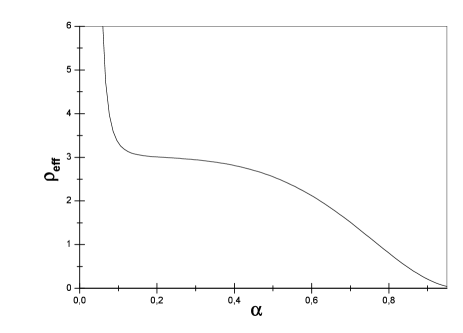
Figure 1: The induced energy density on the brane as a function of the brane scale factor.

4. Cosmological evolution of the Brane-Universe

In the case of non constant dilaton and tachyon the effective energy density using the solutions given by Tseytlin, Klebanov and Minahan [12], [9] is calculated.

We consider again a D3-brane moving along a geodesic in the background of a type 0 string. Having all the solutions in the ultra violet and the infrared, we can follow the cosmological evolution of our universe as it moves along the radial coordinate $r$. In the presence of a non trivial tachyon field the coupling $e^{-\Phi}$ which appears in the Dirac-Born-Infeld action in (2.2), is modified by a tachyonic function $\kappa(T)=1+\frac{1}{4}T+O(T^{2})$. Then we can define an effective coupling [12]

$$e^{-\Phi}_{eff}=\kappa(T)e^{-\Phi}$$ (4.1)

The bulk fields are also coordinate dependent and the induced metric on the brane will depend on a non trivial way on the dilaton field. Therefore the metric in the string frame will be connected to the metric in the Einstein frame through $g_{St}=e^{\frac{\Phi}{2}}_{eff}g_{E}$. All the quantities used so far were defined in the string frame. We will follow our cosmological evolution in the Einstein frame. Then the relation (2.4) becomes

$$\frac{8\pi}{3}\rho_{eff}=(\frac{\dot{\alpha}}{\alpha})^{2}=\frac{(C+E)^{2}g_{S}-|g_{00}|(g_{S}g^{3}+\ell^{2})}{4|g_{00}|g_{rr}g_{S}g^{3}}(\frac{g^{\prime}}{g})^{2}$$ (4.2)

Having the approximate solution in the UV we can calculate the metric components and the $RR$ field C. So, we can calculate the effective energy density from (4.2) setting $\ell^{2}=0$ and we get

$$\frac{8\pi}{3}\rho_{eff} = \Big{[}\Big{(}1-\frac{1}{Q\alpha^{4}}Ei[log2Q+4log\alpha]+\frac{E}{2\alpha^{4}}\Big{)}^{2}$$ (4.3)

$$-\frac{1}{4}\Big{(}1-\frac{1}{2(log2Q+4log\alpha)}\Big{)}^{4}\Big{]}\Big{(}1-\frac{1}{2(log2Q+4log\alpha)}\Big{)}^{-4}\Big{(}1-\frac{9}{2(log2Q+4log\alpha)}\Big{)}^{-1}$$

$$\Big{(}1+\frac{1}{(log2Q+4log\alpha)^{2}}\frac{1}{\Big{(}1-\frac{1}{2(log2Q+4log\alpha)}\Big{)}}\Big{)}^{2}$$

For some typical value of the parameters Q=1 and E=1, and for large values of $\alpha$, it is obvious that $\rho_{eff}$ has a constant value. Therefore an observer on the brane will see an expanding inflating universe. It is interesting to see what happens for small values of $\alpha$. As $\alpha$ gets smaller, a term proportional to $\frac{1}{(\log\alpha)^{4}}$ starts to contribute to $\rho_{eff}$. Therefore the universe for small values of scale factor has a slow expanding inflationary phase which we call it ”logarithmic inflationary” phase. For smaller value of $\alpha$ we cannot trust the solution which is reflected in the fact that $\rho_{eff}$ gets infinite. The behaviour of the effective energy density as a function of the scale factor is shown in Figure 2.

Figure 2: The induced energy density on the brane as a function of the brane scale factor.

To have an idea how the slow inflationary phase proceeds, we can assume for the moment that the effective energy density scales as

$$\frac{8\pi}{3}\rho_{eff}=(\frac{\dot{\alpha}}{\alpha})^{2}=\frac{1}{(\log\alpha)^{p}}$$ (4.4)

The solution of the above equation is

$$\alpha=e^{\textstyle t^{\textstyle(\frac{2}{p+2})}}$$ (4.5)

Therefore we remain in an exponentially growing universe, but various values of p have the effect of making the universe to slow down its expansion. We note here that in order to estimate the behaviour and the duration of this ”logarithmic inflationary” phase, we have to resolve the problem of the singularity.

Going now to IR $\rho_{eff}$ becomes,

$$\frac{8\pi}{3}\rho_{eff} = \Big{[}\Big{(}-1-2\frac{1}{\sqrt{2}Q\alpha^{4}}Ei[log\sqrt{2}Q+4log\alpha]+\frac{E}{\sqrt{2}\alpha^{4}}\Big{)}^{2}-$$ (4.6)

$$\frac{1}{2}\Big{(}1+\frac{9}{2(log\sqrt{2}Q+4log\alpha)}\Big{)}^{4}\Big{]}\Big{(}1+\frac{9}{2(log\sqrt{2}Q+4log\alpha)}\Big{)}^{-4}$$

$$\Big{(}1+\frac{1}{2(log\sqrt{2}Q+4log\alpha)}\Big{)}^{-1}$$

$$\Big{(}1-\frac{9}{2(4log\alpha+log\sqrt{2}Q)^{2}}\frac{1}{\Big{(}1-\frac{9}{2(log\sqrt{2}Q+4log\alpha)}\Big{)}}\Big{)}^{2}$$

As we can see, the above relation is the same as the energy density in the UV (relation (4.3)) up to some numerical factors, as expected. The difference is, that now it is valid for small $\alpha$. For small $\alpha$ first the term $\frac{1}{\alpha^{8}}$ dominates and then the term $\frac{1}{\alpha^{4}}$. As $\alpha$ increases the term $\frac{1}{(\log\alpha)^{4}}$ takes over and drives the universe to a slow inflationary expansion.

5. Discussion

We had followed a probe brane along a geodesic in the background of type 0 string. Assuming that the universe is described by a four-dimensional brane, we calculate the effective energy density which is induced on the brane because of this motion. We study this mirage matter as the brane-universe moves along the radial coordinate.

At first we found, that the motion of the brane-universe in this particular background induces an inflationary phase on the brane. We made the analysis in the limited case where the dilaton and tachyon fields were constants. This assumption simplified the calculation because there is an exact solution of the equations of motion.

We also extended our study to a background where all the fields were functions of the radial coordinate. Using the solutions given by [12], [9], we calculated the energy densities that are induced on the brane. What we found is that for large values of the scale factor as it is measured on the brane (large values of the radial coordinate) the universe enters a slow inflationary phase, in which the energy density is proportional to an inverse power of the logarithm of the scale factor. As the scale factor grows the induced energy density takes a constant value and the universe enters a normal exponential expansion. For small values of the scale factor the induced energy density scales as the inverse powers of the scale factor and then the logarithmic terms take over and the universe enters a slow exponential expansion.

The energy densities we calculated break down for some specific values of the scale factor. This is a reflection of the fact that the approximate solutions in the IR cannot be continued to the UV. To answer the question if there is a true phase of ”logarithmic inflation” in which the universe inflates but with a slow rate, we must resolve the problem of singularities, where our theory breaks down.

References

- [1] T.Regge and C.Teitelboim, Marcel Grossman Meeting on General Relativity,Trieste 1975, North Holland ; V.A. Rubakov and M.E. Shaposhnikov, Do we live inside a domain wall? Phys. Lett.,B 125 (1983) 136 .
- [2] N.Arkani-Hamed, S.Dimopoulos and G.Dvali, The hierarchy problem and new dimensions at a millimeter, Phys. Lett. B 429(1998) 263 [hep-ph/9803315]; Phenomenology, astrophysics and cosmology of theories with submillimeter dimensions and TeV scale quantum gravity, Phys. Rev.D 59 (1999) 086004[hep-ph/9807344]; I.Antoniadis, N.Arkani-Hamed, S.Dimopoulos and G.Dvali, New dimensions at a millimeter to a Fermi and superstrings at a TeV, Phys. Lett. B 436 (1998) 257 [hep-ph/9804398]
- [3] R.Sundrum, Effective field theory for a three-brane universe, Phys. Rev. D 59 (1999) 085009 [hep-ph/9805471]; Compactification for a three brane universe, Phys. Rev. D 59 (1999) 085010 [hep-ph/9807348]; L.Randall and R.Sundrum, Out of this world supersymmetry breaking, Nucl. Phys. B.557 (1999) 79 [hep-th/9810155]; A large mass hierarchy from a small extra dimension, Phys. Rev. Lett. 83 (1999) 3370 [hep-ph/9905221].
- [4] J.Polchinski, Dirichlet branes and Ramond-Ramond charges, Phys. Rev. Lett. 75 (1995) 4724 [hep-th/9510017]
- [5] P.Horava and E.Witten, Heterotic and type-I string dynamics from eleven dimensions, Nucl. Phys. B 460 (1996) 506 [hep-th/9510209]
- [6] H.A.Chamblin and H.S.Reall, Dynamic dilatonic domain walls, hep-th/9903225; A.Chamblin, M.J/Perry and H.S.Reall, Non-BPS D8-branes and dynamic domain walls in massive IIA supergravities, J.High Energy Phys. 09 (1999) 014 [hep-th/9908047]. P.Kraus, Dynamics of Anti-de Sitter Domain Walls, JHEP 9912:011 (1999) [hep-th/9910149]
- [7] A.Kehagias and E.Kiritsis, Mirage cosmology, JHEP 9911:022 (1999) [hep-th/9910174]
- [8] E.Papantonopoulos and I.Pappa, Type 0 Brane Inflation from Mirage Cosmology, [hep-th/0001183]
- [9] J.A.Minahan, Asymptotic Freedom and Confinement from Type 0 String Theory, JHEP 9904:007 (1999) [hep-th/9902074]
- [10] R.Grena,S.Lelli,M.Maggiore,A.Rissone, Confinement,asymptotic freedom and renormalons in type 0 string duals, [hep-th/0005213]
- [11] I.R.Klebanov and A.A.Tseytlin, D-Branes and Dual Gauge Theories in Type 0 Strings, Nucl.Phys. B 546(1999) 155 [hep-th/9811035].
- [12] I.R.Klebanov and A.Tseytlin, Asymptotic Freedom and Infrared Behavior in the type 0 String Approach to gauge theory, Nucl.Phys. B 547 (1999) 143 [hep-th/9812089]
- [13] I.R.Klebanov Tachyon Stabilization in the AdS/CFT Correspondence [hep-th/9906220]
- [14] E.Papantonopoulos and I.Pappa, Cosmological Evolution of a Brane Universe in a Type 0 String Background Phys. Rev. D63 (2001) 103506 [hep-th/0010014]