1 Introduction

Recently, there have been many new examples to resolve singularities in string theory [1]-[22]. (See Ref. [23] for a review of the singularity problem in string theory.) They typically resolve naked singularities.

These works originated from the study of gauge/gravity duals. As a result, many of them are systems with D3-branes, and they have less supersymmetry than the maximal one. The original Maldacena duality is the duality between the type IIB string on $AdS_{5}\times S^{5}$ and $D=4$, ${\cal N}=4$ supersymmetric Yang-Mills theory. It is of course very important to study other duals with less supersymmetry in order to study a more realistic gauge theory and its physics. This is obviously a topic many people have considered, and thus we have many examples. In this case, the background is often $AdS_{5}\times X$ asymptotically, where $X$ is a more general transverse space than the original $S^{5}$. So, naive deformations of $AdS_{5}$ tend to produce singularities, but stringy physics cures the problem.

The singularity in the original geometry is often naked. Moreover, they are “unphysical.” It seems unlikely that one can interpret them as physically reasonable sources. This contrasts with traditional approaches of singularity resolution (e.g., $\alpha^{\prime}$-corrections and orbifolds), where one interprets the singularities as sources. A typical unphysical behavior is that gravitational force becomes repulsive near the singularity. This type of singularity is known as “repulson.” They are unphysical just like the $M<0$ Schwarzschild [24], but the final geometries usually do not have the problem (e.g., all enhançon examples known to date, the Klebanov-Strassler solution, and some of “transgression” examples).

The enhançon mechanism [1] is one of the most studied mechanisms and is applied to many systems [2]-[7]. The prototypical example, the K3-wrapped D$p$-branes for $p=4,\ldots,7$, has been studied further. (See Refs. [25]-[29] for recent discussion.)

For example, the K3-wrapped D6-brane induces a negative D2 tension and charge [30]-[33]. (For that reason, the system is sometimes denoted as D6-D2*.) The naive supergravity solution has a repulson singularity. However, the constituents, the wrapped D6-branes, become massless before reaching the singularity. Thus, the naive supergravity analysis breaks down, and one must take into account stringy physics. Their conclusion is that constituent branes do not form the singularity. Rather, they stay at a finite radius $r=r_{e}$ and form a “shell.” Since all the sources are at this radius, the geometry is flat in the interior. The claim is based on the fact that there is no consistent way to move the branes to $r<r_{e}$ further without contradicting with supersymmetry. This claim is further supported by the ${\cal N}=2$ supersymmetric gauge theory analysis. In the $d=6$ language, a D4-D0* system, which is also massless at $r=r_{e}$, is a W-boson, and the D6-D2* system corresponds to a SU(2) monopole. The fact that the D6-D2* system cannot move inside the enhançon radius has the gauge theory interpretation that the size of the monopole is inversely proportional to the W-boson mass; hence, the brane cannot be localized as $r\rightarrow r_{e}$.

Now, a different string theory realizes this phenomenon by a different mechanism. The type IIA string on K3 is S-dualized to the heterotic string on $T^{4}$, and the phenomenon (for $p=4$) is a consequence of the self-dual radius in this heterotic form; the BPS winding string with $N_{L}=0$ becomes massless when the $S^{1}$ radius the string wraps becomes the string scale $l_{s}$. In fact, the repulson singularity is first discussed in this context [34]-[36]. As another example, a different dual system consists of D$(p-3)$-branes ending on a pair of NS5-branes. In this system, the phenomenon is realized by Myers’ effect, and it has been studied in detail [37].

We study the enhançon mechanism in the heterotic form in detail. The heterotic form has some advantages over the type IIA form. The massless BPS winding string is just a familiar perturbative effect. The heterotic form is also somewhat cleaner since $\alpha^{\prime}$-corrections are under better control. In the type IIA form, the naive D4-D0* solution is just a leading order solution in $\alpha^{\prime}$, so it is not clear whether the repulson geometry is really singular. (However, if $\alpha^{\prime}$-corrections resolved the singularity, one would be left with the unphysical region near the singularity.) In contrast, the solution for the $(1,1)$ string is known to be exact to all orders in $\alpha^{\prime}$[38]-[40], so the singularity survives the $\alpha^{\prime}$-corrections (apart from the $\alpha^{\prime}$-corrections due to source terms [41]). Also, in the type IIA string, the curvature is actually strong near the enhançon radius, which complicates the situation (Sec. 2.1), whereas the curvature remains weak near the enhançon radius in the heterotic form. Finally, in order to obtain the probe action for $r<r_{e}$, Ref. [1] takes the absolute value of the probe Dirac-Born-Infeld action by hand; in the heterotic form, the absolute value appears naturally (Sec. 3.2). In short, the heterotic form strongly supports the picture of Ref. [1]. This work also provides an interesting application of the Kaluza-Klein monopole action [42]-[46], which is rarely discussed in the literature. For other works on the heterotic form, see Refs. [29, 47].

The heterotic form has some disadvantages as well; the analysis in the heterotic string is more involved. The probe analysis is not so simple as the D-brane probe analysis. The D2*-brane effect comes from the higher order corrections in the D-brane action, but the similar corrections for the Kaluza-Klein monopole action are less known. The $d=10$ singularity of the $(1,1)$ string is not a standard curvature singularity, but a parallelly propagated curvature singularity (Sec. 2.2 and App. A).

The organization of the present paper is as follows. In the next section, we describe the backgrounds we study. We show that they are S-dual to the type IIA backgrounds and that they have repulson singularities even from the $d=10$ point of view. We also give the interpretation of those backgrounds [34]-[36], [48]. In Sec. 3, we carry out the probe analysis in those backgrounds. It is also shown that both the “W-boson” and “SU(2) monopole” become massless simultaneously in those backgrounds, which is crucial for the validity of the enhançon mechanism. As in the type IIA cases, the enhançon radii can actually be identified from physical reasoning only. Thus, we first present the heuristic analysis in Sec. 3.1 to identify the enhançon radii, and then we justify the results using the probe actions. This is useful since the probe analysis is somewhat more involved than the type IIA cases.

2 Heterotic Repulsons

2.1 Geometry and Interpretation

We consider a system of $N$ winding strings with momentum, and a system of $N$ Kaluza-Klein dyons [48]. We denote our backgrounds as NS1-W* and KK5-NS5*, respectively, to distinguish them from the standard solutions. However, this is somewhat misleading because the NS1-W* system really corresponds to the $(n,w)=(\pm 1,\pm 1)$ string [34]-[36]. Denote a world-volume direction of a brane by $\times$ and a transverse direction by $-$. Then, the brane configurations we consider in the type IIA string are given by

$$\begin{array}[]{lcc|ccccc|cccc}&&0&1&2&3&4&5&6&7&8&9\\ \hline\cr\mbox{D0*}&&\times&-&-&-&-&-&-&-&-&-\\ \mbox{D4}&&\times&-&-&-&-&-&\times&\times&\times&\times\\ \hline\cr\mbox{D2*}&&\times&-&-&-&\times&\times&-&-&-&-\\ \mbox{D6}&&\times&-&-&-&\times&\times&\times&\times&\times&\times\end{array}$$ (1)

whereas the brane configurations in the heterotic string are given by

$$\begin{array}[]{lcc|ccccc|cccc}&&0&1&2&3&4&5&6&7&8&9\\ \hline\cr\mbox{NS1}&&\times&-&-&-&-&-&-&-&-&\times\\ \mbox{W*}&&\times&-&-&-&-&-&-&-&-&z\\ \hline\cr\mbox{KK5}&&\times&-&-&-&\times&\times&\times&\times&\times&z\\ \mbox{NS5*}&&\times&-&-&-&\times&\times&\times&\times&\times&-\end{array}$$ (2)

The $z$ is the direction of momentum, or the transverse direction of the Kaluza-Klein monopole with no Goldstone mode. The $x^{6},\ldots,x^{9}$ directions are compact in both cases. The D$p$-D$(p-4)^{*}$ systems are compactified on K3, and the NS-brane systems are compactified on $T^{3}\times S^{1}$, where $S^{1}$ is the $z=x^{9}$ direction. There are basically three relative alignments of the NS1-W* and KK5-NS5* branes. The NS1-W* system may be aligned

1. with the world-volume directions of the KK5-NS5* system ($x^{4},\ldots,x^{8}$),

2. with the transverse directions ($x^{1},\ldots,x^{3}$), or

3. with the isometry direction $z$.

The important configuration is the last of these since both the NS1-W* and KK5-NS5* branes give extra massless spectra from the configuration.

The D$p$-D$(p-4)^{*}$ solution is given by

$$ds^{2} = Z_{p-4}^{-1/2}Z_{p}^{-1/2}\eta_{mn}\,dx^{m}dx^{n}+Z_{p-4}^{1/2}Z_{p}^{1/2}dx^{i}dx^{i}+v_{A}^{1/2}Z_{p-4}^{1/2}Z_{p}^{-1/2}ds^{2}_{\rm K3},$$

$$e^{-2\phi} = \frac{1}{g_{A}^{2}}Z_{p-4}^{-(7-p)/2}Z_{p}^{(p-3)/2},$$

$$C_{p-3} = \frac{1}{g_{A}}(Z_{p-4}^{-1}-1)\,dx^{0}\wedge dx^{10-p}\wedge\cdots\wedge dx^{5},$$

$$C_{p+1} = \frac{1}{g_{A}}(Z_{p}^{-1}-1)\,dx^{0}\wedge dx^{10-p}\wedge\cdots\wedge dx^{9}.$$ (3)

Here, $m,n$ run over the directions tangent to all the branes, and $i$ runs over the directions transverse to all branes. The metric $ds^{2}_{\rm K3}$ is a K3 surface metric of volume $(2\pi l_{s})^{4}$, and the K3 volume is

$$V_{A} = (2\pi l_{s})^{4}v_{A},$$

$$v_{A} = R_{6A}\ldots R_{9A}$$ (4)

in the orbifold limit. Namely, we measure the compact volume in units of $2\pi l_{s}$, which makes T-duality rules simple. All compact spatial coordinates run from 0 to $2\pi l_{s}$. (All world-volume coordinates also run from 0 to $2\pi l_{s}$.) The coupling constant in the type IIA (heterotic) string is denoted as $g_{A}$ ($g_{h}$). Then, the harmonic functions are given by

$$\begin{array}[]{cclccl}Z_{0}&=&\displaystyle{1-\frac{|r_{0}|^{3}}{r^{3}}},&r_{0}^{3}&=&\displaystyle{\frac{\pi g_{A}Nl_{s}^{3}}{v_{A}}},\\ Z_{4}&=&\displaystyle{1+\frac{r_{4}^{3}}{r^{3}}},&r_{4}^{3}&=&\pi g_{A}Nl_{s}^{3}\end{array}$$ (5)

for the D4-D0* case ($r^{2}=x^{i}x^{i}$), and

$$\begin{array}[]{cclccl}Z_{2}&=&\displaystyle{1-\frac{|r_{2}|}{r}},&r_{2}&=&\displaystyle{\frac{g_{A}Nl_{s}}{2v_{A}}},\\ Z_{6}&=&\displaystyle{1+\frac{r_{6}}{r}},&r_{6}&=&\displaystyle{\frac{g_{A}Nl_{s}}{2}}\end{array}$$ (6)

for the D6-D2* case.

Similar to Ref. [1], we simply analytically continue a harmonic function of a brane. The heterotic/IIA S-duality guarantees that such systems should exist, but the interpretation is given later. The branes with * are chosen so that the total mass is positive when the $S^{1}$ radius is large. Then, the NS1-W* solution is given by

$$ds^{2} = f_{1}^{-1}\{-dt^{2}+R^{2}dz^{2}+(f_{n}-1)(dt-Rdz)^{2}\}+dx^{i}dx^{i}+v_{3}^{2/3}ds^{2}_{T^{3}},$$

$$e^{-2\phi} = \frac{1}{g_{h}^{2}}\,f_{1},$$

$$B_{2} = (f_{1}^{-1}-1)\,dt\wedge(Rdz),$$ (7)

where

$$\begin{array}[]{cclccl}f_{1}&=&\displaystyle{1+\frac{r_{1}^{3}}{r^{3}}},&r_{1}^{3}&=&\displaystyle{\frac{\pi g_{h}^{2}Nl_{s}^{3}}{v_{h}}R},\\ f_{n}&=&\displaystyle{1-\frac{|r_{n}|^{3}}{r^{3}}},&r_{n}^{3}&=&\displaystyle{\frac{\pi g_{h}^{2}Nl_{s}^{3}}{v_{h}}\frac{1}{R}}.\end{array}$$ (8)

The torus volume is defined similar to the type IIA cases; $ds^{2}_{T^{3}}$ is the $T^{3}$-metric of volume $(2\pi l_{s})^{3}$, $R=R_{9h}$, and

$$V_{h} = (2\pi l_{s})^{4}v_{h},$$

$$v_{h} = Rv_{3}.$$ (9)

The KK5-NS5* solution is given by

$$ds^{2} = \eta_{mn}dx^{m}dx^{n}+f_{5}\left\{f_{K}(dr^{2}+r^{2}d\Omega_{2}^{2})+f_{K}^{-1}R^{2}(dz+A_{\varphi}d\varphi)^{2}\right\}+v_{3}^{2/3}ds^{2}_{T^{3}},$$

$$e^{-2\phi} = \frac{1}{g_{h}^{2}}\,f_{5}^{-1},$$

$$A_{1} = \frac{r_{K}}{R}(1-\cos\theta)\,d\varphi,$$

$$B_{2} = -r_{5}(1-\cos\theta)\,d\varphi\wedge(Rdz),$$ (10)

where

$$\begin{array}[]{cclccl}f_{5}&=&\displaystyle{1-\frac{|r_{5}|}{r}},&r_{5}=\displaystyle{\frac{Nl_{s}}{2}\frac{1}{R}},\\ f_{K}&=&\displaystyle{1+\frac{r_{K}}{r}},&r_{K}=\displaystyle{\frac{Nl_{s}}{2}R}.\end{array}$$ (11)

The gravitational wave W* is no more an anti-wave than the D2*-brane is an anti-D2-brane. The anti-wave is just a parity reflection $z\rightarrow-z$ of the original system. The solution does not change and is uninteresting. Rather, the NS1-W* system is interpreted as a true $(n,w)=(1,1)$ string [34]-[36]. In Sec. 3.2, we indeed see that a $(1,1)$ probe string has a flat potential in this background, but a $(-1,1)$ probe string does not. Also, recall the mass-shell conditions for the heterotic string:

$$\mbox{right-moving (NS-sector): }\quad m^{2} = P_{R}^{2}+\frac{4}{l_{s}^{2}}(N_{R}-\frac{1}{2}),$$

$$\mbox{left-moving: }\quad m^{2} = P_{L}^{2}+\frac{4}{l_{s}^{2}}(N_{L}-1),$$ (12)

where $P_{L,R}=(n/R\pm wR)/l_{s}$. The BPS states are those with one world-sheet fermion $\psi_{-1/2}^{\mu}$ excited or $N_{R}=1/2$. Thus, the $(1,1)$ string has the mass $m^{2}=(R-1/R)^{2}/l_{s}^{2}$. This mass formula coincides with the NS1-W* mass $M\sim r_{1}^{3}-r_{n}^{3}\sim R-1/R$. Thus, roughly speaking, the effective negative energy from W* comes from the Casimir energy. At the self-dual radius $R=1$, the massless spectrum is given by $(N_{L},n,w)=(1,0,0),(0,\pm 1,\pm 1)$, and they form an enhanced SU(2) gauge symmetry.

The NS5*-brane tension and charge are induced by the KK5-brane curvature due to the heterotic anomaly equation [47, 48]:

$$H_{3}=dB_{2}+\frac{l_{s}^{2}}{4}\left(\omega_{3}^{L}(\Omega)-\frac{1}{30}\omega_{3}^{YM}(A)\right),$$ (13)

where $\omega_{3}^{L}$ and $\omega_{3}^{YM}$ are the Lorentz and Yang-Mills Chern-Simons three-forms. The Lorentz Chern-Simons term induces $(-1)$ unit of NS5-brane charge since a Kaluza-Klein monopole has $(+1)$ unit of gravitational instanton number. The backreaction of the NS5*-geometry on Eq. (13) is subleading in $1/R$ (higher orders in $\alpha^{\prime}$). Since the system is a BPS object, its tension should also be modified appropriately.

The above result, however, assumes weak curvature. Since the heterotic anomaly equation (13) could get higher order corrections in $\alpha^{\prime}$, the issue of $\alpha^{\prime}$-corrections may arise. If $\alpha^{\prime}$-corrections become important, the background solution (10) could not be reliable as well. However, the curvature remains weak in the region we are interested in, namely near the enhançon radii (Sec. 3.1). More importantly, the weak curvature result continues to hold due to the standard charge quantization and the BPS condition [47].

A similar point arises for type IIA cases as well. Near the enhançon radii, the size of K3 is about the string scale $l_{s}$. Since K3 is curved, the curvature near the enhançon radius generally becomes strong, so the $\alpha^{\prime}$-corrections are not negligible. This could have changed the results of Ref. [1]. The K3-wrapped D6-brane has $(-1)$ unit of D2-brane charge, but the analysis takes into account only the leading $\alpha^{\prime}$-corrections in the Dirac action and in the Chern-Simons coupling. The actions should have higher order corrections in $\alpha^{\prime}$, and those corrections may invalidate the weak curvature result. In particular, the naive D6-D2* probe action would not make sense. However, the K3-wrapped D6-brane continues to have $(-1)$ unit of D2-brane charge even in the large curvature region due to the charge quantization. Thus, the effective probe action itself is still reliable, but the D6-D2* background may be modified.

2.2 Repulson Singularities

The heterotic systems are S-dual to the type IIA ones, so their $d=6$ geometries have the same repulson behaviors (in the Einstein metric). Here, we examine repulson singularities from the $d=10$ point of view. It is sometimes stated that the NS1-W* geometry is regular at $r=r_{n}$, but we will see this is not the case.

For the KK5-NS5* background, the Ricci scalar is

$$R_{\rm KK5-NS5^{*}}=\frac{3r_{5}^{2}}{2(r-r_{5})^{3}(r+r_{K})},$$ (14)

so it is singular at $r=r_{5}$, but the Ricci scalar of the NS1-W* background is finite at $r=r_{n}$:

$$R_{\rm NS1-W^{*}}=-\frac{63r_{1}^{6}}{2r^{2}(r^{3}+r_{1}^{3})}.$$ (15)

However, one cannot immediately conclude that the NS1-W* geometry is regular at $r=r_{n}$. First of all, singularities at which curvature invariants diverge are not the only singularities that could appear. In general relativity, one can classify singularities as follows [49]:

1. s.p. (scalar polynomial) curvature singularities;

2. p.p. (parallelly propagated) curvature singularities;

3. others (the conical singularity, Taub-NUT space, …).

The singularity such as the KK5-NS5* system corresponds to type (i), but it is well known that the singularity of the plane wave corresponds to type (ii). All curvature invariants remain finite for the background, but it still has a diverging tidal force (see, e.g., Ref. [50]). This holds for more general cases, and the singularity due to momentum cannot be seen from curvature invariants only [51]. Thus, one had better be careful to check singularities when one adds momentum. A proper way to see the singularity is to compute the Riemann tensor components in parallelly propagated frames. Note that the tidal force is proportional to the Riemann tensor from the equation of geodesic deviation. Since its components are frame-dependent, it is important to determine a natural frame to see them. One natural frame is the rest frame of an infalling observer, which is known as a parallelly propagated frame (a frame obtained by the parallel-transport along the observer’s geodesic). In App. A, we show that the NS1-W* geometry has a p.p. curvature singularity at $r=r_{n}$.

These singularities are repulson singularities from the motion of minimally-coupled massive particles. The potential wall becomes infinitely repulsive when harmonic functions of branes with * vanish. The existence of Killing vectors $\xi=\partial_{t},\partial_{z}$ implies conserved charges $p\cdot\xi$ or $E=-p_{0}/m$ and $P=p_{z}/m$, where $E$ and $P$ are the energy and momentum along $S^{1}$ per unit mass, respectively. For simplicity, we consider the motion in the $z-r$ plane only and set the other conserved charges to zero. Then, the radial motion is given by

$$\frac{dr}{d\tau} = \pm\sqrt{-G^{00}G_{rr}^{-1}}\sqrt{2(\tilde{E}-V_{\rm eff})},$$

$$2V_{\rm eff} = (-G^{00})^{-1}(1+P^{2}G^{zz}),$$ (16)

where $\tilde{E}=E^{2}/2$. For the NS1-W* geometry, the potential $V_{\rm eff}$ is attractive asymptotically. It begins to be repulsive at

$$r^{3}=\frac{2R^{2}}{R^{2}-1}|r_{n}|^{3},$$ (17)

and becomes infinitely strong at the singularity. The effective potential for the KK5-NS5* geometry is flat at zero momentum since $G_{00}$ is flat, but it has an infinitely repulsive potential wall at $r=r_{5}$ for $P\neq 0$.

In many recent examples of the singularity resolution, the singularity in the original geometry is not only naked, but also repulsive. In fact, a repulsive singularity is timelike for a general static spherically symmetric metric (App. B). Thus, it is at least “locally naked” (like the Reissner-Nordström singularity) or “globally naked.”

2.3 HET/IIA Duality

Under the $d=6$ heterotic/IIA S-duality, the NS1-W* system is dual to the D4-D0* system, and the KK5-NS5* system to the D6-D2* system. The Kaluza-Klein procedure is standard:

$$\mbox{$d$-dimensional dilaton:}\quad\phi \rightarrow \sigma=\phi-\frac{1}{4}\ln\det G_{c},$$

$$\mbox{$d$-dimensional metric:}\quad G_{\mu\nu} \rightarrow G_{\mu\nu}^{\prime}=G_{\mu\nu}-G_{zz}^{-1}G_{\mu z}G_{\nu z},$$

$$\mbox{Einstein metric:}\quad G_{\mu\nu}^{E} = e^{-\frac{4\sigma}{d-2}}G_{\mu\nu}^{\prime},$$ (18)

where $G_{c}$ is the metric of a compact space. After rescaling the coordinates $t$ and $r$, the compactified type IIA branes are

$$ds_{E}^{2} = -(Z_{0}Z_{4})^{-3/4}dt^{2}+(Z_{0}Z_{4})^{1/4}(dr^{2}+r^{2}d\Omega_{4}^{2}),$$

$$e^{-2\sigma_{A}} = \frac{v_{A}}{g_{A}^{2}}(Z_{0}Z_{4})^{-1/2},$$ (19)

$$ds_{E}^{2} = (Z_{2}Z_{6})^{-1/4}(-dt^{2}+\cdots)+(Z_{2}Z_{6})^{3/4}(dr^{2}+r^{2}d\Omega_{2}^{2}),$$

$$e^{-2\sigma_{A}} = \frac{v_{A}}{g_{A}^{2}}(Z_{2}Z_{6})^{1/2},$$ (20)

whereas the heterotic branes are

$$ds_{E}^{2} = -(f_{1}f_{n})^{-3/4}dt^{2}+(f_{1}f_{n})^{1/4}(dr^{2}+r^{2}d\Omega_{4}^{2}),$$

$$e^{-2\sigma_{h}} = \frac{v_{h}}{g_{h}^{2}}(f_{1}f_{n})^{1/2},$$ (21)

$$ds_{E}^{2} = (f_{5}f_{k})^{-1/4}(-dt^{2}+\cdots)+(f_{5}f_{k})^{3/4}(dr^{2}+r^{2}d\Omega_{2}^{2}),$$

$$e^{-2\sigma_{h}} = \frac{v_{h}}{g_{h}^{2}}(f_{5}f_{k})^{-1/2}.$$ (22)

Becasue of the scaling, the supergravity parameters are scaled as well:

$$\begin{array}[]{cclccl}r_{0}^{3}&=&\pi Nl_{s}^{3}(g_{A}^{2}v_{A})^{-1/4},&r_{4}^{3}&=&\displaystyle{\pi Nl_{s}^{3}\left(\frac{v_{A}^{3}}{g_{A}^{2}}\right)^{1/4}},\\ r_{2}&=&\displaystyle{\frac{Nl_{s}}{2}\left(\frac{g_{A}^{2}}{v_{A}^{3}}\right)^{1/4}},&r_{6}&=&\displaystyle{\frac{Nl_{s}}{2}(g_{A}^{2}v_{A})^{1/4}},\\ r_{1}^{3}&=&\displaystyle{\pi Nl_{s}^{3}\left(\frac{g_{h}^{2}R^{4}}{v_{h}}\right)^{1/4}},&r_{n}^{3}&=&\displaystyle{\pi Nl_{s}^{3}\left(\frac{g_{h}^{2}}{R^{4}v_{h}}\right)^{1/4}},\\ r_{5}&=&\displaystyle{\frac{Nl_{s}}{2}\left(\frac{v_{h}}{g_{h}^{2}R^{4}}\right)^{1/4}},&r_{K}&=&\displaystyle{\frac{Nl_{s}}{2}\left(\frac{R^{4}v_{h}}{g_{h}^{2}}\right)^{1/4}}.\end{array}$$ (23)

The S-duality is given by $G_{\mu\nu}^{E}\,{\rm(IIA)}=G_{\mu\nu}^{E}\,{\rm(HET)},\sigma_{A}=-\sigma_{h}$ with

$$g_{A} = g_{h}^{-1}R_{9h}v_{h}^{1/2},$$

$$R_{9A} = v_{h}^{-1/2}R_{9h},$$

$$R_{mA} = v_{h}^{1/2}R_{mh}^{-1},\qquad m=6,7,8$$ (24)

in the orbifold limit of K3 [52]. The type IIA branes (19) and (20) are dual to the heterotic branes (21) and (22), respectively, under the duality. Since the $d=6$ Einstein metric is invariant under the S-duality, both the KK5-NS5* and NS1-W* backgrounds clearly have s.p. curvature singularities at $r=r_{5}$ and $r=r_{n}$, respectively, after the reduction.

3 Brane Probes

3.1 Heuristic Analysis

In the D6-D2* system, the enhançon radius can be identified from physical reasoning only. Here, we first make such a heuristic analysis for the heterotic string.

First recall the D$p$-D$(p-4)^{*}$ system. The tension of the $d=6$ effective $(p-4)$-brane is given by

$$\tau=\frac{N}{g_{A}}(\mu_{p}V_{A}-\mu_{p-4})=\frac{N}{g_{A}}\mu_{p}(V_{A}-V_{*}),$$ (25)

where $V_{*}=(2\pi)^{4}l_{s}^{4}$ and

$$\mu_{p}=\frac{1}{(2\pi)^{p}l_{s}^{p+1}}.$$ (26)

The D$p$-D$(p-4)^{*}$ probes all become massless at the same place $V_{A}=V_{*}$, which is crucial for the validity of the enhançon mechanism. The $p=4,6$ systems are the W-boson and SU(2) monopole, respectively, in the $d=6$ gauge theory language. Since the monopole mass is proportional to the W-boson mass, their mass must vanish simultaneously. We see below that the NS1-W* and KK5-NS5* systems also have vanishing mass at the same radii.

In the curved background, the K3 volume $V_{A}$ varies with position, so replace $V_{A}$ with the invariant volume $V(r)$. Then, D-brane probes become massless at $V(r)=V_{*}$, namely at

$$r=\frac{2V_{A}}{V_{A}-V_{*}}|r_{2}|,$$ (27)

which is the right answer from the brane probe analysis.

Now, the mass of the BPS string is given by

$$\tau=\frac{n}{R}-wR.$$ (28)

The KK5-NS5* tension is given by

$$\tau=\frac{1}{g_{h}^{2}}\mu_{5}(Q_{K}R^{2}-Q_{5}).$$ (29)

The mass of a KK5-brane, $m=R_{4}\cdots R_{8}R^{2}/(g_{h}^{2}l_{s})$, can be determined from the T-dual of the NS5 tension or using the Dirac quantization condition. The tensions are positive for the choice $R>1$ when $n=w=N$ and $Q_{5}=Q_{K}=N$.

First, consider the NS1-W* background. Changing $R$ to the invariant $S^{1}$ radius $R(r)=R\sqrt{f_{n}/f_{1}}$, we find that the $(n,w)=(\pm 1,\pm 1)$ strings become massless when

$$f_{n}R^{2}=f_{1}\quad{\rm or}\quad r^{3}=\frac{2R^{2}}{R^{2}-1}|r_{n}|^{3}=r_{e}^{3}.$$ (30)

The invariant radius becomes $R(r_{e})=1$ at the enhançon radius. Note that the KK5-NS5* tension (29) has the same form as the NS1-W* one (28), so the KK5-NS5* probe becomes massless at the same radius. Thus, the repulsive region (17) is actually excised by the enhançon mechanism like the D6-D2* case. The effective potential analysis in Sec. 2.2 is of course frame-dependent, and it is not very clear which frame one must choose [12, 25]. If one uses the Einstein metric, not all repulsive regions are excised. (This is true for the D6-D2* case as well.)

Similarly, the invariant $S^{1}$ radius is $R(r)=R\sqrt{f_{5}/f_{K}}$ for the KK5-NS5* background, and the enhançon radius is given by

$$f_{5}R^{2}=f_{K}\quad{\rm or}\quad\tilde{r}_{e}=\frac{2R^{2}}{R^{2}-1}|r_{5}|$$ (31)

for both the NS1-W* and KK5-NS5* probes.

It is easy to check that both the curvature and coupling remain weak at enhançon radii. For the NS1-W* background,

$$R|_{r_{e}}\rightarrow-\frac{63}{2l_{s}^{2}}\left(\frac{Rv_{h}}{2\pi g_{h}^{2}N}\right)^{2/3},\quad e^{2\phi}|_{r_{e}}=g_{h}^{2}\,\frac{2}{R^{2}+1}.$$ (32)

The above Ricci scalar is for the limiting case $R\gg 1$. For the KK5-NS5* background,

$$R|_{\tilde{r}_{e}}=\frac{6}{N^{2}l_{s}^{2}}\left(\frac{R^{2}-1}{R^{2}+1}\right)^{4},\quad e^{2\phi}|_{\tilde{r}_{e}}=g_{h}^{2}\,\frac{R^{2}+1}{2R^{2}}.$$ (33)

When $R>1$, they remain weak in the large-$N$ limit, $g_{h}\rightarrow 0,N\rightarrow\infty$ with $g_{h}^{2}N\gg 1$. One can also check that the Riemann tensor in a p.p. frame remains weak for the NS1-W* case. On the contrary, the curvature is in general not weak in the type IIA form due to the hidden K3 curvature.

3.2 NS1-W* Probe

The Lorentzian form of the $\sigma$-model action is given by

$$S_{\sigma}=-\frac{1}{4\pi l_{s}^{2}}\int d^{2}\sigma\sqrt{-h}\left(h^{ab}\partial_{a}X^{\mu}\partial_{b}X^{\nu}G_{\mu\nu}-\epsilon^{ab}\partial_{a}X^{\mu}\partial_{b}X^{\nu}B_{\mu\nu}\right),$$ (34)

where $\epsilon^{01}=1/\sqrt{-h}$ and $\epsilon_{01}=-\sqrt{-h}$. All world-volume coordinates run from 0 to $2\pi l_{s}$. The NS1-W probe analysis in the NS1-W background has been carried out in Refs. [53, 54] in the weak field approximation.

Our gauge choice and ansatz are as follows:

$$X^{0} = \tau,$$

$$X^{9} = X^{9}(\tau,\sigma)=\sigma+y(\tau),$$

$$X^{i} = X^{i}(\tau),$$

$$h_{\tau\tau} = h_{\tau\tau}(\tau),$$

$$h_{\sigma\sigma} = h_{\sigma\sigma}(\tau),$$

$$h_{\tau\sigma} = 0.$$ (35)

In this ansatz, the string has a unit winding. The conformal gauge cannot be taken because the background breaks the SO(1,1) invariance on the world-sheet due to the plane wave. (Recall $h_{ab}\propto g_{ab}$ by solving $h_{ab}$ equations of motion, where $g_{ab}$ is the induced metric.) The action then becomes

$$S_{\sigma}=-\frac{2\pi l_{s}}{4\pi l_{s}^{2}}\int d\tau\left(-e^{-1}G_{\mu\nu}\dot{X}^{\mu}\dot{X}^{\nu}+eG_{99}+2B_{\mu 9}\dot{X}^{\mu}\right),$$ (36)

where $e\equiv\sqrt{-h_{\tau\tau}/h_{\sigma\sigma}}$. The $y$ is a cyclic coordinate, so there is a conserved momentum:

$$P\equiv\frac{\partial L}{\partial\dot{y}}=\frac{1}{2l_{s}e}(2\dot{y}G_{99}+2G_{\hat{\mu}9}\dot{X}^{\hat{\mu}}),$$ (37)

where the sum on $\hat{\mu}$ does not include 9. One can substitute back $P$ into the action and eliminate $y$ by using the Routhian [55]. The Routhian is defined as $R\equiv P\dot{y}-L\rightarrow-L^{\prime}$:

$$S^{\prime}_{\sigma} = -\frac{1}{2l_{s}}\int d\tau\left\{e^{-1}\left(-G_{\hat{\mu}\hat{\nu}}\dot{X}^{\hat{\mu}}\dot{X}^{\hat{\nu}}+\frac{(G_{\hat{\mu}9}\dot{X}^{\hat{\mu}})^{2}}{G_{99}}\right)\right.$$ (38)

$$\left.+e\left(G_{99}+\frac{P^{2}l_{s}^{2}}{G_{99}}\right)-\left(2B_{\hat{\mu}9}+2l_{s}\frac{PG_{\hat{\mu}9}}{G_{99}}\right)\dot{X}^{\hat{\mu}}\right\}.$$

As shown in Ref. [53], to properly take into account the Casimir energy, the correct constraint equation is as follows:

$$T_{ab}=-\frac{1}{l_{s}^{2}}\left(\begin{array}[]{cc}e^{2}&e\\ e&1\end{array}\right).$$ (39)

Imposing the off-diagonal element of the constraint determines $P$:

$$P=\frac{1}{l_{s}}.$$ (40)

Meanwhile, the diagonal element gives the correct mass-shell condition (12) for the $X^{\hat{\mu}}$-independent terms in Eq. (38):

$$e\left(G_{99}+\frac{1}{G_{99}}\right)\rightarrow eG_{99}\left(1-\frac{1}{G_{99}}\right)^{2}.$$ (41)

After eliminating $e$ using its equation of motion, we can expand the action in powers of transverse velocity as

$$l_{s}\times{\cal L}^{\prime}_{\sigma} = -\left|Rf_{1}^{-1}-\frac{1}{R}f_{n}^{-1}\right|+\frac{1}{2R}|f_{n}R^{2}-f_{1}|v^{2}$$ (42)

$$\hskip 36.135pt+R(f_{1}^{-1}-1)-\frac{1}{R}(f_{n}^{-1}-1)+\cdots$$

$$= -\frac{R^{2}-1}{R}+\frac{1}{2R}(f_{n}R^{2}-f_{1})v^{2}+\cdots$$ (43)

in the NS1-W* background. We have taken $r>r_{e}$ in the last line. The potential is flat, and the effective mass takes the form as expected from the heuristic analysis (30). This analysis also shows that the NS1-W* system really corresponds to the $(n,w)=(1,1)$ string. Just as the D6-D2* analysis, the effective mass could be negative for $r<r_{e}$ if the second term in Eq. (42) is not an absolute value. But it is clear in the heterotic side that this is actually spurious. The tension is always positive as expected. However, as discussed in Ref. [1], the potential no longer cancels in this case, thus the probe at $r<r_{e}$ contradicts with supersymmetry. Therefore, the probe actually cannot go inside $r_{e}$.

Similarly, in the KK5-NS5* background (for $r>\tilde{r}_{e}$),

$$l_{s}\times{\cal L}^{\prime}_{\sigma}=-\frac{f_{5}R^{2}-f_{K}}{R\sqrt{f_{5}f_{K}}}+\frac{1}{2R}(f_{5}R^{2}-f_{K})\sqrt{f_{5}f_{K}}v^{2}+\cdots.$$ (44)

The effective mass again agrees with the heuristic analysis (31), and the potential is of course not flat for this case.

3.3 KK5-NS5* Probe

The actions for Kaluza-Klein branes in string/M-theory have been discussed in Refs. [42]-[46]. For the heterotic string, the KK5 probe action is given by [42, 43]

$$S_{\rm KK5}=-\mu_{5}\int d^{6}\sigma e^{-2\phi}k^{2}\sqrt{-\det(\Pi_{ab}+k^{-2}F_{a}F_{b})}+S_{\rm WZ}.$$ (45)

Here, $g_{ab}$ is the induced metric; the pull-back of tensors is always denoted with indices $a,b,\ldots$. Also,

$$k^{2} = k^{\mu}k^{\nu}G_{\mu\nu}=G_{zz},$$

$$\Pi_{ab} = g_{ab}-k^{-2}k_{a}k_{b},$$

$$F_{a} = \partial_{a}s+\partial_{a}X^{\mu}k^{\nu}B_{\mu\nu},$$ (46)

where $k\equiv(\partial_{z})^{\mu}$ is the Killing vector associated to the isometry direction $z$ of the probe KK-brane, and the field $s$ is a world-volume scalar. The factor $k^{2}$ in the kinetic term is a characteristic of the Kaluza-Klein monopole and accounts for the factor $R^{2}$ of the tension in Eq. (29). The actions are proportional to $\mu_{5}$; the string coupling $g_{s}$ is included in the background solutions (7) and (10). Some references often include $g_{s}$ in tensions, not in backgrounds (e.g., Ref. [52]). When the background metric has an off-diagonal element between the isometry direction $z$ and a direction parallel to the probe brane, $k_{a}\neq 0$ in general. This is actually the case for the W*-background for the configuration (2).

The relevant term of the Wess-Zumino action is

$$S_{\rm WZ}=\mu_{5}\int d^{6}\sigma\,\frac{\sqrt{-g}}{6!}\epsilon^{a_{0}\cdots a_{5}}\,k^{\mu}\partial_{a_{0}}X^{\mu_{0}}\cdots\partial_{a_{5}}X^{\mu_{5}}\,A_{\mu\mu_{0}\cdots\mu_{5}}$$ (47)

(the full Wess-Zumino action is given in Ref. [43]), where $dA_{7}=k^{2}e^{-2\phi}*dA_{1}$ or

$$F_{\mu_{1}\cdots\mu_{8}} = \frac{1}{2!}\,k^{2}e^{-2\phi}\epsilon_{\mu_{1}\cdots\mu_{10}}F^{\mu_{9}\mu_{10}},$$ (48)

$$A_{\mu} = k^{-2}k^{\nu}G_{\mu\nu}.$$ (49)

The NS5 probe action is given by [56]

$$S_{\rm NS5}=-\mu_{5}\int d^{6}\sigma e^{-2\phi}\sqrt{-\det g_{ab}}+\mu_{5}\int B_{6},$$ (50)

where $dB_{6}=e^{-2\phi}*dB_{2}$. In principle, the effective NS5*-brane action could be derived from higher order corrections of the Kaluza-Klein monopole action in a manner similar to the effective D6-D2* action. Here, we take the actions (50) and (45) as our starting point since these corrections are less known.

For the KK5-NS5* background, one can choose a static gauge:

$$X^{0} = \tau,$$

$$X^{9} = 0,$$

$$X^{a+3} = \sigma^{a},\qquad a=1,\ldots,5,$$

$$X^{i} = X^{i}(\tau).$$ (51)

Using the small velocity approximation, we get the KK5-NS5* probe action as

$${\cal L}=-v_{3}(\tau_{\rm KK5}+\tau_{\rm NS5^{*}})+\frac{1}{2}\,v_{3}(\tau_{\rm KK5}f_{5}+\tau_{\rm NS5^{*}}f_{K})v^{2}+\cdots.$$ (52)

For the NS1-W* background, the gauge choice and ansatz are

$$X^{0} = \tau,$$

$$X^{9} = \tilde{y}(\tau),$$

$$X^{a+3} = \sigma^{a},\qquad a=1,\ldots,5,$$

$$X^{i} = X^{i}(\tau).$$ (53)

The $\tilde{y}$ is again a cyclic coordinate, so there is a conserved momentum $\tilde{P}$. Since we want the probe KK5-NS5* brane to carry no momentum, $\tilde{P}=0$. Substituting this back to the action, we get the KK5-NS5* probe action as

$${\cal L}=-v_{3}\frac{\tau_{\rm KK5}f_{n}+\tau_{\rm NS5^{*}}f_{1}}{\sqrt{f_{1}f_{n}}}+\frac{1}{2}\,v_{3}(\tau_{\rm KK5}f_{n}+\tau_{\rm NS5^{*}}f_{1})\sqrt{f_{1}f_{n}}v^{2}+\cdots.$$ (54)

Again the results (52) and (54) agree with the heuristic analyses.

As a check, the probe results we obtained (43), (44), (52), and (54) are consistent with various dualities. For instance, consider the D6-D2* background in the type IIA string. The effective particle action from the D4-D0* probe is given by

$${\cal L}_{\rm D4-D0^{*}}=-\frac{\mu_{4}V_{A}Z_{2}-\mu_{0}Z_{6}}{g_{A}\sqrt{Z_{2}Z_{6}}}+\frac{1}{2g_{A}}(\mu_{4}V_{A}Z_{2}-\mu_{0}Z_{6})\sqrt{Z_{2}Z_{6}}v^{2}+\cdots.$$ (55)

The effective membrane action from the D6-D2* probe is given by

$${\cal L}_{\rm D6-D2^{*}}=-\frac{\mu_{6}V_{A}-\mu_{2}}{g_{A}}+\frac{1}{2g_{A}}(\mu_{6}V_{A}Z_{2}-\mu_{2}Z_{6})v^{2}+\cdots.$$ (56)

Equations (44) and (52) are S-dual to (55) and (56), respectively. The heterotic results are also invariant under the T-duality $R\rightarrow 1/R$.

Appendix A The p.p. Singularity in the NS1-W* Geometry

The p.p. singularity has been discussed in various works; see, e.g., Refs. [51, 57] for recent discussions in the context of string theory. Standard textbooks in general relativity often have a treatment; see, e.g., Chap. 31.2 of Ref. [58] for an elementary introduction. We mostly follow the notations and the derivation of Ref. [51]. Many equations are unchanged, but the final result is not the same. This is because the reference focuses on the standard branes whose geometry could be singular only at $r=0$.

A p.p. singularity is the one where the Riemann tensor components are unbounded in a p.p. frame along at least one non-spacelike curve. The calculation consists of three steps: (i) First, choose a timelike geodesic (an infalling observer) along which we calculate the Riemann tensor; (ii) Then, choose a convenient frame to calculate the Riemann tensor, and find the transformation which relates the frame to the observer’s frame; (iii) Finally, transform the Riemann tensor to the observer’s frame to obtain the observer’s tidal forces.

(i) Geodesics: We denote the metric as

$$ds^{2}=2F_{2}\,dudv+F_{3}^{2}du^{2}+F_{1}^{-2}dx^{i}dx^{i},$$ (57)

where $z=u+v$ and $t=v$. For the NS1-W* geometry, $F_{1}=1,F_{2}=f_{1}^{-1}$, and $F_{3}^{2}=f_{1}^{-1}f_{n}$. The geodesic equation leads to the ten-velocity of the observer $V^{\mu}=dx^{\mu}/d\tau$, where

$$\frac{du}{d\tau} = \frac{P-E}{F_{2}},\qquad\frac{dv}{d\tau}=\frac{P}{F_{2}}+\left(\frac{F_{3}}{F_{2}}\right)^{2}(E-P)^{2},$$ (58)

$$(\frac{dr}{d\tau})^{2} = (E-P)^{2}\left(\frac{F_{1}F_{3}}{F_{2}}\right)^{2}+\frac{2F_{1}^{2}}{F_{2}}(E-P)P-F_{1}^{2}.$$ (59)

Here, $E$ and $P$ are the integrals of motion. We also fix the motion in the $u-r$ plane only, which is consistent with the other components of the geodesic equation.

(ii) Lorentz transformation: The Riemann tensor $R^{klmn}$ may be first computed not in the observer’s frame [with coordinates $(\hat{\tau},\hat{x},\hat{\rho},\ldots)$], but in a stationary orthonormal frame [with coordinates $(\hat{0},\hat{4},\hat{r},\ldots)$]:

$$e^{\hat{0}}=\frac{F_{2}}{F_{3}}dv,\qquad e^{\hat{4}}=F_{3}du+\frac{F_{2}}{F_{3}}dv,\qquad e^{\hat{r}}=F_{1}^{-1}dr.$$ (60)

The Riemann tensor in the observer’s frame is then obtained by a Lorentz boost. For the NS1-W* geometry, the Riemann tensor components diverge as $r\rightarrow r_{n}$ at this level. The components may not diverge for other p.p. singularities, and the singularity may appear as the result of the boost.

The ten-velocity in this frame is given by $V^{a}=e^{a}_{~{}\mu}V^{\mu}$, where

$$V^{\hat{0}} = \frac{F_{3}}{F_{2}}(E-P)+\frac{P}{F_{3}},\qquad V^{\hat{4}}=\frac{P}{F_{3}},$$ (61)

$$V^{\hat{r}} = \pm\left\{\left(\frac{F_{3}}{F_{2}}\right)^{2}(E-P)^{2}+\frac{2(E-P)P}{F_{2}}-1\right\}.$$ (62)

Now, the Lorentz transformation we need takes a unit timelike vector $N^{a}=\delta^{a}_{~{}\hat{0}}$ (the observer’s ten-velocity in his own frame) into $V^{a}$ (the ten-velocity in the stationary frame), so $V^{a}=L^{a}_{~{}b}N^{b}$. One simple choice of such a SO(1,9) matrix is

$$L^{a}_{~{}b}=\left(\begin{array}[]{cccc}V^{\hat{0}}&V^{\hat{4}}&V^{\hat{r}}&{\hat{0}}\\ V^{\hat{4}}&1+\frac{(V^{\hat{4}})^{2}}{V^{\hat{0}}+1}&\frac{V^{\hat{4}}V^{\hat{r}}}{V^{\hat{0}}+1}&0\\ V^{\hat{r}}&\frac{V^{\hat{4}}V^{\hat{r}}}{V^{\hat{0}}+1}&1+\frac{(V^{\hat{r}})^{2}}{V^{\hat{0}}+1}&0\\ 0&0&0&1\end{array}\right),$$ (63)

where 1 is an identity matrix. Strictly speaking, the frame obtained by the transformation may differ from the parallelly propagated frame by a rotation, but it suffices to see the singularity.

(ii) Tidal forces: Finally, apply the Lorentz transformation (63) to the Riemann tensor in the stationary frame $R^{klmn}$; $R^{abcd}=L^{a}_{~{}k}L^{b}_{~{}l}L^{c}_{~{}m}L^{d}_{~{}n}R^{klmn}$. This gives the tidal forces for the observer. For the NS1-W* background, the leading terms as $r\rightarrow r_{n}$ for some components are

$$R^{\hat{x}\hat{\rho}\hat{x}\hat{\rho}},\hat{R}^{\hat{\tau}\hat{\rho}\hat{\tau}\hat{\rho}},\hat{R}^{\hat{x}\hat{\rho}\hat{\tau}\hat{\rho}}\rightarrow\frac{2P^{2}(r_{1}^{3}+4r_{n}^{3})}{3r_{n}^{3}(r-r_{n})^{2}},$$ (64)

$$R^{\hat{\tau}\hat{x}\hat{\tau}\hat{x}}\rightarrow\frac{-2(r_{1}^{3}+4r_{n}^{3})\{r_{n}^{3}+2P^{2}(r_{1}^{3}+r_{n}^{3})-2PE(r_{1}^{3}+r_{n}^{3})\}}{r_{n}^{4}(r_{1}^{3}+r_{n}^{3})(r-r_{n})}.$$ (65)

This shows that the NS1-W* geometry has a p.p. curvature singularity at $r=r_{n}$.

Appendix B Repulson and Naked Singularity

Here, we limit ourselves to a general static spherically symmetric metric in $n$-dimensions:

$$ds^{2}=-f^{2}(r)dt^{2}+f(r)^{-2}dr^{2}+R(r)^{2}d\Omega_{n-2}^{2}.$$ (66)

Then, the repulsive singularities must be timelike. The argument goes as follows. From Eq. (16), the effective potential is $V_{\rm eff}=f^{2}$. So, an infinite repulsive potential means that $f^{2}\rightarrow\infty$ or $G_{00}\rightarrow-\infty$ as $r\rightarrow 0$, where we chose that $r=0$ is the singularity. Thus, $f$ never has a zero near the singularity. Now, define a new radial coordinate $r_{*}=\int f^{-2}dr$ and null coordinates $u=t-r_{*}$, $v=t+r_{*}$. Then the two-dimensional part of the metric reads as $ds_{2}^{2}=-f^{2}dudv$. Now, the causal structure of the singularity is as follows:

1. If one can choose the integration constant so that $r_{*}=0$ at $r=0$ and if $f^{2}>0$, then the singularity is timelike.

2. Same as above, but if $f^{2}<0$, it is spacelike.

3. If $r_{*}=-\infty$ at $r=0$, it is null.

Because $f$ never has a zero near the singularity and $f^{2}>0$ in our case, it is timelike. Therefore, it must be either locally naked, i.e., surrounded by a horizon, or globally naked, i.e., a true naked singularity.

Even though repulsive singularities are timelike, the converse is not true. The standard D6-brane has a timelike singularity which is attractive. This is because repulsive behavior is not necessary in order to have $r_{*}=0$ at the singularity. One could have $f\sim r^{a}$, where $a<1/2$ (for the D6-brane, $a=1/4$). Another example is the cosmic string with a conical space.

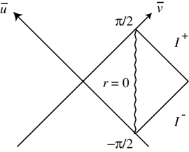
Figure 1: The Penrose diagram in the local patch.

The above causal structures can be checked by drawing the resulting Penrose diagram. The new null coordinates

$$\tan\bar{u}=-e^{-u},\quad\tan\bar{v}=e^{v},\quad\mbox{where }|\bar{u}|<\pi/2,|\bar{v}|<\pi/2$$ (67)

transforms the metric into

$$ds_{2}^{2}=-f^{2}\sec^{2}\bar{u}\sec^{2}\bar{v}d\bar{u}d\bar{v}.$$ (68)

When $f^{2}>0$, the Penrose diagram then looks like Fig. 1 in the local patch.

References

- [1] C. V. Johnson, A. W. Peet and J. Polchinski, “Gauge theory and the excision of repulson singularities,” Phys. Rev. D61 (2000) 086001 [arXiv:hep-th/9911161].
- [2] A. Buchel, A. W. Peet and J. Polchinski, “Gauge dual and noncommutative extension of an supergravity solution,” Phys. Rev. D 63 (2001) 044009 [arXiv:hep-th/0008076].
- [3] N. Evans, C. V. Johnson and M. Petrini, “The enhançon and gauge theory/gravity RG flows,” JHEP 0010 (2000) 022 [arXiv:hep-th/0008081].
- [4] M. Bertolini, P. Di Vecchia, M. Frau, A. Lerda, R. Marotta and I. Pesando, “Fractional D-branes and their gauge duals,” JHEP 0102 (2001) 014 [arXiv:hep-th/0011077].
- [5] J. Polchinski, “ gauge-gravity duals,” Int. J. Mod. Phys. A 16 (2001) 707 [arXiv:hep-th/0011193].
- [6] M. Frau, A. Liccardo and R. Musto, “The geometry of fractional branes,” Nucl. Phys. B 602 (2001) 39 [arXiv:hep-th/0012035].
- [7] P. Merlatti, “The enhançon mechanism for fractional branes,” arXiv:hep-th/0108016.
- [8] J. Polchinski and M. J. Strassler, “The string dual of a confining four-dimensional gauge theory,” arXiv:hep-th/0003136.
- [9] R. C. Myers and O. Tafjord, “Superstars and giant gravitons,” arXiv:hep-th/0109127.
- [10] I. R. Klebanov and A. A. Tseytlin, “Gravity duals of supersymmetric SU(N) SU(N+M) gauge theories,” Nucl. Phys. B 578 (2000) 123 [arXiv:hep-th/0002159].
- [11] I. R. Klebanov and M. J. Strassler, “Supergravity and a confining gauge theory: duality cascades and SB-resolution of naked singularities,” JHEP 0008 (2000) 052 [arXiv:hep-th/0007191].
- [12] J. Maldacena and C. Nunez, “Supergravity description of field theories on curved manifolds and a no-go theorem,” Int. J. Mod. Phys. A 16 (2001) 822 [arXiv:hep-th/0007018].
- [13] L. A. Pando Zayas and A. A. Tseytlin, “3-branes on resolved conifold,” JHEP 0011 (2000) 028 [arXiv:hep-th/0010088].
- [14] M. Cvetic, H. Lu and C. N. Pope, “Brane resolution through transgression,” Nucl. Phys. B 600 (2001) 103 [arXiv:hep-th/0011023].
- [15] F. Cachazo, K. Intriligator and C. Vafa, “A large duality via a geometric transition,” Nucl. Phys. B 603 (2001) 3 [arXiv:hep-th/0103067].
- [16] J. D. Edelstein, K. Oh and R. Tatar, “Orientifold, geometric transition and large duality for SO/Sp gauge theories,” JHEP 0105 (2001) 009 [arXiv:hep-th/0104037].
- [17] M. Atiyah and E. Witten, “M-theory dynamics on a manifold of holonomy,” arXiv:hep-th/0107177.
- [18] P. Kraus, F. Larsen and S. P. Trivedi, “The Coulomb branch of gauge theory from rotating branes,” JHEP 9903 (1999) 003 [arXiv:hep-th/9811120].
- [19] D. Z. Freedman, S. S. Gubser, K. Pilch and N. P. Warner, “Continuous distributions of D3-branes and gauged supergravity,” JHEP 0007 (2000) 038 [arXiv:hep-th/9906194].
- [20] A. Brandhuber and K. Sfetsos, “Wilson loops from multicentre and rotating branes, mass gaps and phase structure in gauge theories,” Adv. Theor. Math. Phys. 3 (1999) 851 [arXiv:hep-th/9906201].
- [21] R. Kallosh, T. Mohaupt and M. Shmakova, “Excision of singularities by stringy domain walls,” arXiv:hep-th/0010271.
- [22] A. Adams, J. Polchinski and E. Silverstein, “Don’t panic! Closed string tachyons in ALE space-times,” arXiv:hep-th/0108075.
- [23] M. Natsuume, “The singularity problem in string theory,” gr-qc/0108059.
- [24] G. T. Horowitz and R. Myers, “The value of singularities,” Gen. Rel. Grav. 27 (1995) 915 [arXiv:gr-qc/9503062].
- [25] C. V. Johnson, R. C. Myers, A. W. Peet and S. F. Ross, “The enhançon and the consistency of excision,” Phys. Rev. D 64 (2001) 106001 [arXiv:hep-th/0105077].
- [26] C. V. Johnson and R. C. Myers, “The enhançon, black holes, and the second law,” Phys. Rev. D 64 (2001) 106002 [arXiv:hep-th/0105159].
- [27] N. R. Constable, “The entropy of 4D black holes and the enhancon,” Phys. Rev. D 64 (2001) 104004 [arXiv:hep-th/0106038].
- [28] K. Maeda, T. Torii, M. Narita and S. Yahikozawa, “The stability of the shell of D2-D6 branes in a supergravity solution,” arXiv:hep-th/0107060.
- [29] M. Wijnholt and S. Zhukov, “Inside an enhançon: monopoles and dual Yang-Mills Theory,” arXiv:hep-th/0110109.
- [30] M. Bershadsky, C. Vafa and V. Sadov, “D-branes and topological field theories,” Nucl. Phys. B 463 (1996) 420 [arXiv:hep-th/9511222].
- [31] M. B. Green, J. A. Harvey and G. W. Moore, “I-brane inflow and anomalous couplings on D-branes,” Class. Quant. Grav. 14 (1997) 47 [arXiv:hep-th/9605033].
- [32] K. Dasgupta, D. P. Jatkar and S. Mukhi, “Gravitational couplings and orientifolds,” Nucl. Phys. B 523 (1998) 465 [arXiv:hep-th/9707224].
- [33] C. P. Bachas, P. Bain and M. B. Green, “Curvature terms in D-brane actions and their M-theory origin,” JHEP 9905 (1999) 011 [arXiv:hep-th/9903210].
- [34] K. Behrndt, “About a class of exact string backgrounds,” Nucl. Phys. B 455 (1995) 188 [arXiv:hep-th/9506106].
- [35] R. Kallosh and A. Linde, “Exact supersymmetric massive and massless white holes,” Phys. Rev. D 52 (1995) 7137 [arXiv:hep-th/9507022].
- [36] M. Cvetic and D. Youm, “Singular BPS saturated states and enhanced symmetries of four-dimensional supersymmetric string vacua,” Phys. Lett. B 359 (1995) 87 [arXiv:hep-th/9507160].
- [37] C. V. Johnson, “Enhançons, fuzzy spheres and multi-monopoles,” Phys. Rev. D 63 (2001) 065004 [arXiv:hep-th/0004068].
- [38] G. T. Horowitz and A. A. Tseytlin, “On exact solutions and singularities in string theory,” Phys. Rev. D 50 (1994) 5204 [arXiv:hep-th/9406067].
- [39] G. T. Horowitz and A. A. Tseytlin, “Extremal black holes as exact string solutions,” Phys. Rev. Lett. 73 (1994) 3351 [arXiv:hep-th/9408040].
- [40] G. T. Horowitz and A. A. Tseytlin, “A New class of exact solutions in string theory,” Phys. Rev. D 51 (1995) 2896 [arXiv:hep-th/9409021].
- [41] A. A. Tseytlin, “On singularities of spherically symmetric backgrounds in string theory,” Phys. Lett. B363 (1995) 223 [arXiv:hep-th/9509050].
- [42] E. Bergshoeff, B. Janssen and T. Ortin, “Kaluza-Klein monopoles and gauged sigma-models,” Phys. Lett. B 410 (1997) 131 [arXiv:hep-th/9706117].
- [43] B. Janssen, “A T-duality approach to the gravitational wave and the Kaluza-Klein monopole,” Fortsch. Phys. 47 (1999) 201.
- [44] E. Bergshoeff, Y. Lozano and T. Ortin, “Massive branes,” Nucl. Phys. B 518 (1998) 363 [arXiv:hep-th/9712115].
- [45] E. Bergshoeff, E. Eyras and Y. Lozano, “The massive Kaluza-Klein monopole,” Phys. Lett. B 430 (1998) 77 [arXiv:hep-th/9802199].
- [46] E. Eyras, B. Janssen and Y. Lozano, “5-branes, KK-monopoles and T-duality,” Nucl. Phys. B 531 (1998) 275 [arXiv:hep-th/9806169].
- [47] M. Krogh, “S-duality and tensionless 5-branes in compactified heterotic string theory,” JHEP 9912 (1999) 018 [arXiv:hep-th/9911084].
- [48] A. Sen, “Kaluza-Klein dyons in string theory,” Phys. Rev. Lett. 79 (1997) 1619 [arXiv:hep-th/9705212].
- [49] F. J. Tipler, C. J. S. Clarke, and G. F. R. Ellis, “Singularities and horizons - a review article,” in General relativity and gravitation: one hundred years after the birth of Albert Einstein, edited by A. Held (Plenum, New York, 1980).
- [50] G. T. Horowitz and A. R. Steif, “Spacetime singularities in string theory,” Phys. Rev. Lett. 64 (1990) 260.
- [51] N. Kaloper, R. C. Myers and H. Roussel, “Wavy strings: black or bright?,” Phys. Rev. D 55 (1997) 7625 [arXiv:hep-th/9612248].
- [52] J. Polchinski, String theory (Cambridge University Press, Cambridge, England, 1998).
- [53] J. P. Gauntlett, J. A. Harvey, M. M. Robinson and D. Waldram, “Scattering of macroscopic heterotic strings,” Nucl. Phys. B 411 (1994) 461 [arXiv:hep-th/9305066].
- [54] C. G. Callan, J. M. Maldacena and A. W. Peet, “Extremal black holes as fundamental strings,” Nucl. Phys. B 475 (1996) 645 [arXiv:hep-th/9510134].
- [55] H. Goldstein, Classical mechanics (Addison-Wesley, Reading, MA, 1980); L. D. Landau, Mechanics (Pergamon, Oxford, 1976).
- [56] C. G. Callan, J. A. Harvey and A. Strominger, “Worldbrane actions for string solitons,” Nucl. Phys. B 367 (1991) 60.
- [57] G. T. Horowitz and H. s. Yang, “Black strings and classical hair,” Phys. Rev. D 55 (1997) 7618 [arXiv:hep-th/9701077].
- [58] C. W. Misner, K. S. Thorne, and J. A. Wheeler, Gravitation (Freeman, San Francisco, 1973).