Brane-Antibrane Inflation in Orbifold and Orientifold Models

Abstract:

We analyse the cosmological implications of brane-antibrane systems in string-theoretic orbifold and orientifold models. In a class of realistic models, consistency conditions require branes and antibranes to be stuck at different fixed points, and so their mutual attraction generates a potential for one of the radii of the underlying torus or the 4D string dilaton. Assuming that all other moduli have been fixed by string effects, we find that this potential leads naturally to a period of cosmic inflation with the radion or dilaton field as the inflaton. The slow-roll conditions are satisfied more generically than if the branes were free to move within the space. The appearance of tachyon fields at certain points in moduli space indicates the onset of phase transitions to different non-BPS brane systems, providing ways of ending inflation and reheating the corresponding observable brane universe. In each case we find relations between the inflationary parameters and the string scale to get the correct spectrum of density perturbations. In some examples the small numbers required as inputs are no smaller than 0.01, and are the same small quantities which are required to explain the gauge hierarchy.

1 Introduction

Recent observations are beginning to redundantly test the standard Big-Bang picture of late-time cosmology, and the success of this theoretical description is determining the values which are required for the various cosmological parameters. The success sharpens the need to understand the puzzling initial conditions of this picture, which are typically cast as various ‘problems’—such as the flatness, horizon and cosmological-constant problems.

Inflationary cosmology [1] represents the potentially cleanest explanation of many of these initial-condition problems—particularly in its hybrid variant [2]—since it recasts the special initial conditions of late-time cosmology as the robust consequences of earlier dynamics which results in the dramatic expansion of the universe. This explanation predicts properties for the temperature fluctuations in the cosmic microwave background (CMB), and quite generically successfully describes the spectrum found by extant observations. There are problems, however, and inflation remains a successful cosmology seeking a convincing theoretical realization. Although considerable latitude exists in model building, since the physics of the relevant scales is largely unknown, fine tuning is generically required in order to obtain sufficient inflation (while also allowing inflation to end at some point) and to describe the small amplitude of the observed temperature fluctuations in the CMB.

It is natural to look to string theory to explain the unnaturally small numbers required by inflation, since it purports to describe the relevant scales, and is arguably our only known consistent description of gravity at the shortest distances. Unfortunately, string realizations of inflation have proven hard to find, partly due to the difficulty in identifying the inflaton from among the plethora of string states, and partly due to the difficulty of obtaining de Sitter solutions to the low-energy effective field equations. Recently, however, a string-based inflationary scenario, based on brane-antibrane attraction and subsequent collision and annihilation, was proposed [3], which circumvents some of these difficulties (see also [4] for related work). The proposal has the following successes:

• The relevant brane-antibrane interaction arises at string tree-level, and so is explicitly calculable once the low-energy spectrum of the model is known.

• Inflation naturally ends once the brane-antibrane separation is of order the string scale, since at this point one of the open-string modes becomes tachyonic, opening up a new direction along which fields may roll. This furnishes a string-theory realization of the hybrid-inflation scenario.

• An explanation is suggested for the dimension of the branes which survive to late times, by attributing these to be the end products of a cascade of earlier brane-antibrane annihilations.

This mechanism provides a geometrical realization of inflation in terms of the position of branes and antibranes. It also hints at new approaches to early-Universe cosmology, in which the initial features of late-time cosmology are understood in terms of the fundamental objects of string theory.

Of course, many questions also remain open within this scenario. Probably the most pointed issue concerns the assumption that the geometric moduli and dilaton field are frozen by some unknown string physics at higher energies (perhaps the string scale). Although it is certainly a logical possibility that these fields are fixed at the string scale without affecting the rest of the low-energy cosmology, no such construction has actually been made.

Next, the brane-antibrane collisions considered in [3] only provided inflation for special initial conditions: parallel branes colliding head-on starting from antipodal points within purely toroidal compactifications. Although some of these special conditions were argued in [3] to arise plausibly from earlier brane evolution, others seem difficult to arrange in this way.

Finally, the known purely toroidal compactifications do not lead to phenomenologically realistic models with chiral matter, and so are not of the most interest from a purely practical perspective of being known to contain vacua which resemble our observed low-energy world.

In this paper we propose an extension of the brane-antibrane inflationary scenario, which extends the analysis of [3] to address the open questions just mentioned. We introduce two new changes in order to do so. First, instead of using the inter-brane separation as inflaton, we now use one of the extra-dimensional moduli for this purpose. Second, we generalize the scenario from toroidal to orbifold compactifications, motivated by the observation that these contain a class of realistic string models. In particular, explicit D-brane models within string theory have been constructed which contain the standard model (or the left-right symmetric model) spectrum among the massless states on the observable brane, including realistic features such as three chiral families, proton stability and gauge coupling unification [5, 6].

We find that brane-antibrane interactions within these models have cosmological interpretations along the lines of ref. [3], but with many improved features. Among these are:

• We find an almost generic occurrence of slow-roll inflation, with the newly-liberated modulus of the extra dimensions as the inflaton;

• We find that the small numbers required by inflationary scenarios may be naturally explained without introducing numbers into the underlying brane theory which are smaller than $\epsilon\sim 0.01$. This happens because the cosmologically relevant quantities arise as large powers of the small parameters of the underlying brane physics. Better yet, the small quantities $\epsilon$ turn out to be precisely the same small quantities which have been used to explain the gauge hierarchy problem [7].

• Inflationary exit occurs because of the intervention of stringy physics, and not due to the violation of the slow-roll conditions for the inflaton. Indeed some of the inflaton potentials we find would not be considered viable if taken on their own, outside of string theory, since they would appear to predict perpetual inflation.

These improvements are suggested by the following interesting feature of the realistic models: consistency conditions (the requirement of tadpole cancellations) force the existence of a number of branes which are trapped at some of the singular fixed-points of the orbifold, with another (different) number of antibranes trapped at other orbifold fixed points.

Since these branes and antibranes are naturally trapped at the fixed points, the separation between them can only be changed by adjusting the size of the extra dimensions. Consequently we must now imagine that this modulus is not fixed, and instead is light enough to play the role of the inflaton field. Notice that the interbrane separation and breathing modes have interchanged their roles compared with ref. [3]—the separation now being fixed and the breathing mode being the inflaton. Our finding that slow-roll inflation becomes generic follows from the change in kinetic energy which is implied by this interchange.

Another interesting consequence of the tadpole-cancellation conditions in these models is the requirement of a mismatch between the number of branes and antibranes, with branes and antibranes localized at different orbifold points. If the extra dimensions shrink due to brane-antibrane attraction, it follows that the endpoint cannot involve complete annihilation, since conservation laws must require the existence of some remnant branes. Once a realistic final state is identified at low energies after inflation, this property may help understand why any branes at all survive into the late universe.

The remaining sections are organized as follows. The next section describes the brane configurations of interest, and identifies their properties which are relevant to inflation. Section 3 then describes the effective four-dimensional theory, and makes contact with standard inflationary phenomenology. Our conclusions are then briefly summarized in section 4. A calculation, which is used en passant, is given in an Appendix.

2 The Underlying String Model

For concreteness we restrict our attention to Type-I, II string configurations in which the six compact dimensions make up an orbifold, which we take to be a product of three 2-dimensional tori whose radii we denote by $r_{i},i=1,2,3$. We keep track of these three radii, and the dilaton, $e^{\phi}$, as the moduli which are of potential cosmological interest at low energies.

2.1 Branes at Orbifold Points

In orientifold and orbifold models there are more types of BPS and non-BPS branes than in toroidal compactifications. In particular there are the so-called fractional branes which are simply branes trapped at one fixed point of the orbifold. Following the realistic orbifold constructions, we populate our spacetime with D9 and D5 branes, and their antibranes, and we take the 5-branes to be fixed at various orbifold points in the extra dimensions. (For some purposes it is convenient to also consider orientifold planes.) $T$-duality relates these configurations to those with D7 and D3 branes.

General tools exist for the construction of such models [8], where the trapping of branes and antibranes at the singular fixed points is required by cancellation of tadpoles at these points. In terms of the effective 4D theory the trapping of the branes is needed in order to have anomaly cancellation, therefore it is clear that otherwise the corresponding string model would be inconsistent.

This class of models has been studied thoroughly during the past few years and they offer a very interesting avenue towards obtaining a realistic model from string theory. In particular it has been shown that models with three families and the standard model gauge group or its left-right generalization can be obtained in this way and supersymmetry is broken by the presence of both branes and antibranes [5, 6], which is realistic if the corresponding string scale is intermediate [7]. Furthermore these models allow the unification of gauge couplings at that scale [5, 9], providing the first explicit string compactifications with gauge-coupling unification and proton stability.

For concreteness, a typical model of this sort we have in mind is a ${\bf Z}_{3}$ orientifold model with 27 fixed points. The standard model lies inside a stack of 3-branes at one of the fixed points, which are themselves immersed inside a stack of 7-branes (which covers 9 of the fixed points). Cancellation of RR tadpoles then requires also two stacks of anti 7-branes, each covering 9 other fixed points, and separated from the 7-branes that contain the standard model. This provides a realization of gravity-mediated supersymmetry breaking with a realistic low-energy spectrum. This picture has a (probably less clear) $T$-dual version in terms of the D5 and D9 branes with Wilson lines [6].

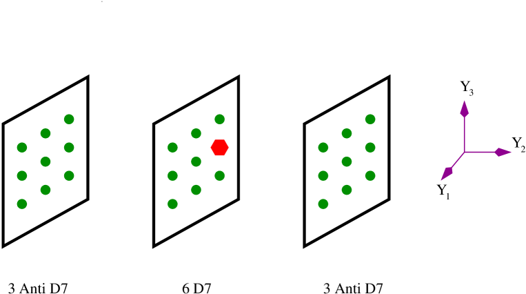
Figure 1: A ‘realistic’ model as in reference [6]. Here we present the 6 extra dimensions in terms of three complex coordinates $Y_{i}$. The standard model is at a stack of D3 branes sitting in one of the 27 fixed points of the ${\bf Z}_{3}$ orbifold, represented here by the red hexagon. The other fixed points are the green dots where other D3 branes may live but the details are not important for us. The standard model 3 branes live inside a stack of 7-branes. There are also anti 7-branes which are trapped at the fixed planes due to tadpole cancellation conditions. The attraction of the branes and antibranes generates a potential for the radius of the torus transverse to the D7-branes similar to what it is considered in the text.

Since the interbrane separation, $y$, is no longer a low-energy degree of freedom, it is frozen within the effective theory. We assume the same to be true of most of the other would-be moduli and the dilaton (more about this later). Most importantly, we do not imagine all of those moduli to be frozen, so at least one of them appears within the low-energy effective theory, and the attractive brane-antibrane potential should be regarded as being a function of that modulus instead of $y$.

2.2 Relevant Approximations

Since we claim our results to be consistent with the low-energy limit of string theory, there are several approximations which we must make. We enunciate these approximations explicitly here, because their failure signals the breakdown of the effective field theory on which our inflationary analysis is based. In later sections we look for situations where these approximations are driven to fail, and interpret this failure as signalling the end of inflation.

From the string point of view the two approximations we make are the low-energy limit, and weak coupling. The first of these is required because we shall work purely within the low-energy field theory, and so require all of the relevant distances—like the extra-dimensional sizes, $r_{i}$, and interbrane separations—to be much larger than the string scale, $M_{s}r\gg 1$. The weak-coupling approximation, $e^{\phi}\ll 1$, is required to the extent that we use string perturbation theory to identify the particle spectrum or to compute interbrane interactions.

Within the low-energy (but higher-dimensional) effective field theory, these approximations typically justify a classical calculation using the linearized field equations. For instance, recalling that $d$ denotes the number of compact dimensions, loop effects in the field theory are controlled by the dimensionless parameter

$${G_{d}\over r^{d+2}}\sim{e^{2\phi}\over(M_{s}r)^{d+2}},$$ (1)

where $G_{d}$ is the higher-dimensional Newton’s constant. The conditions $e^{\phi}\ll 1$ and $M_{s}r\gg 1$ ensure that this parameter is small. Similarly, the approximation of working within near-flat extra-dimensional geometries relies on the neglect of the gravitational (and other) fields for which the various branes act as a source. This neglect is controlled by the dimensionless parameter

$${G_{d}{\cal T}_{p}\over r^{d_{\perp}-2}}\sim{e^{\phi}\,N\over(M_{s}r)^{d_{\perp}-2}},$$ (2)

where $d_{\perp}$ is the number of dimensions transverse to the brane of interest, and we take the $p$-brane tension to be of order ${\cal T}_{p}\sim Ne^{-\phi}M_{s}^{p+1}$, with $N$ denoting the number of coincident branes which source the fields. Unless $N$ is excessively large, this quantity is also small if $e^{\phi}\ll 1$ and $M_{s}r\gg 1$.

Notice that $d_{\perp}-2=d-p+1=(d+2)-(p+1)<d+2$ for all $p>0$, so $M_{s}r\gg 1$ implies $G_{d}{\cal T}_{p}/r^{d_{\perp}-2}\gg G_{d}/r^{d+2}$. It follows that as $r$ decreases it is the nonlinear corrections to the classical field equations which become important before loop effects do. For a fixed $r$, the nonlinear classical effects can always be made important without doing the same for loop effects simply by making $N$ sufficiently large. Indeed, having multiple branes at each point is not an uncommon occurrence within the realistic orbifold models, but even for large $N$ our analysis using the linearized equations applies for sufficiently large $r$.

2.3 Inter-brane Interactions

We now consider how the energetics of a multi-brane configuration depends on the radii, $r_{i}$ and $e^{\phi}$, with an eye to finding those terms which determine how these moduli evolve in the low-energy theory. For widely-separated branes at weak coupling this energetics is dominated by the brane tensions and by the leading inter-brane interactions, which we now describe.

The exchange of bulk states which are approximately massless in the higher-dimensional effective field theory dominates the interactions of widely-separated branes at weak coupling. When the interbrane separation itself is the inflaton [3], these interactions give the leading contribution to the inflaton potential, since this is the leading term in the system energy which depends on the inflaton. This is no longer the case if the inflaton is a modulus, since then the interbrane interaction must also compete with the brane tensions (as we discuss in more detail below).

Consider for simplicity the attractive potential for a parallel $p$-brane/antibrane pair separated by a distance $y$ which is large compared to the string scale $1/M_{s}$. In an infinite transverse space the interaction potential (per unit brane volume) would be:

$$W(y)=-{B\over y^{{d_{\perp}}-2}},$$ (3)

with

$$B={\beta e^{2\phi}\over M_{s}^{2+d}}\,{\cal T}_{p}^{2}\,$$ (4)

where ${d_{\perp}}$ is the number of dimensions perpendicular to the branes: ${d_{\perp}}=d-p+3$ where $d$ is the number of compact extra dimensions.

The constant $\beta$ is a dimensionless number which characterizes the overall strength of the inter-brane force, and depends on the number and types of bulk states which are effectively massless, and so whose exchange generates a power-law potential. For instance, direct D-brane calculation gives the result corresponding to the exchange of the massless states of 10-dimensional supergravity  [10], giving

$$\beta=\pi^{-{d_{\perp}}/2}\Gamma\left[\frac{{d_{\perp}}-2}{2}\right]\,.$$ (5)

The potential of eq. (3) is not directly applicable to a compact manifold like a torus (or orbifold). For instance, for a square torus of size $r$ the periodic boundary conditions imply the potential can be written as the infinite sum of image branes at equivalent lattice points, giving [3]:

$$W({\bf y})\,=\,-\,\sum_{i}\,{B\over|{\bf y}-{\bf y}_{i}|^{{d_{\perp}}-2}}\,,$$ (6)

where $\bf y$ gives the location of the antibrane and the sum is over the location of the infinite image branes located at the lattice points. A similar expression applies for more complicated tori.

In what follows we wish to follow the potential as a function of moduli like $r$, rather than the interbrane separation, $y$. In the present instance this is most easily found by scaling $r$ out of the coordinates, in which case eq. (6) implies

$$W(r)\ =\ -\frac{BG(\xi_{*})}{r^{{d_{\perp}}-2}}$$ (7)

where $B$ are the same constants as before, and $G(\xi)$ is the Green’s function for a massless field on the torus expressed in terms of the rescaled coordinates $\xi^{i}=y^{i}/r$. We imagine $G(\xi)$ to be normalized so that it approaches $1/|\vec{\xi}|^{d_{\perp}-2}$ in the limit that the brane and antibrane approach one another: $\xi\to 0$.

Similar formulae also apply for other combinations of parallel $p$-branes, such as a $D5$ brane and a parallel orientifold 5-plane, $O5$. The only difference in this case would be in the precise value—and sign—taken by $B$. For our purposes this value, and the value of $G(\xi_{*})$, need not concern us, so long as their product is ${\cal O}(1)$ and does not vanish. Ultimately $B$ depends both on the type of branes involved and on the number and types of massless particles whose exchange generates the potential, and generally does not vanish except for supersymmetric BPS-brane configurations. The value for $G(\xi_{*})$ is also nonzero, and is computed explicitly in the Appendix for a simple example of square torus, corresponding to a brane-antibrane configuration on a $Z_{2}$ orbifold, as in Figure (2).

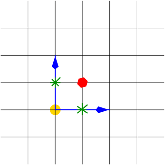
Figure 2: A picture of the ${\bf Z}_{2}$ orbifolds we are considering for cosmological purposes, with branes and antibranes trapped at different fixed points. Of the 4 fixed points shown there the yellow circle represents a stack of branes, the red hexagon a stack of antibranes and the other two fixed points are empty.

Actually $G(\xi)$ also depends on the other moduli of the torus, and leaving it as a free parameter allows us to consider how the interaction energy depends on these variables. We emphasize that a potential like (7) should also apply to the cases of most phenomenological interest, including the ${\bf Z}_{3}$ orbifold of the six dimensional torus discussed earlier.

3 The Effective 4D Theory

We now turn to the effective 4D theory which describes the cosmology of the model. The main assumption on which such a 4D analysis rests is that inflation occurs on scales which are small enough that Kaluza Klein (KK) modes are not excited as inflation proceeds.

There is another, less obvious, condition for the validity of this kind of 4D analysis which we must also impose. Besides working within the 4D theory, we only allow a single field to be rolling during inflation, and this is only justified to the extent that the modulus we choose is the only 4D mode which is excited. In particular, we must assume that other moduli are fixed by physics at higher scales, such as at the string scale. If not, these other moduli could also roll and we would have to re-evaluate whether the universe’s evolution is dominated by the scalar potential rather than the kinetic energies of these other modes. Although string cosmology is likely to involve more moduli than just the single one which we liberate here, we regard our present calculation to be the first (encouraging) step in relaxing the frozen-moduli assumptions that are implicit in the extant string cosmology proposals, including that ref. [3].

With these caveats in mind, we require the 4D effective theory which describes the low-energy dynamics of the brane configuration whose dynamics is of interest. Consider for this purpose the 6-torus described earlier. The brane configuration of interest has two parts. We imagine first having $N_{9}$ $D9$ and $\overline{D9}$ branes, which are stabilized against mutually annihilating by some mechanism. (This might be accomplished, for instance, if there were Wilson lines within the $D9$ but not the $\overline{D9}$, leading to these two 9-branes not carrying precisely opposite values for all conserved charges.) We supplement these with a collection of $N_{5}$ parallel $D5$ branes which are localized at an orbifold point of the four dimensions whose radii are $r_{2}$ and $r_{3}$, and which wrap the two compact $r_{1}$ directions. Parallel to these we also take $N_{5}$ $\overline{D5}$ branes which are located at another orbifold point which is displaced relative to the first in the transverse four dimensions.

3.1 Identifying the 4D Moduli

Although the radii, $r_{i}$, and dilaton, $e^{\phi}$, are moduli in perturbation theory, we imagine that all moduli but one combination of these is fixed by (unknown) physics at scales above the compactification scale. Since the inflation we find in the low-energy theory depends on which combination of moduli is not fixed by this physics—leaving it free to play the role of the inflaton in the low-energy theory—we pause briefly here to motivate the choice we will make.

Since the compactification scales to which we will be led are much larger than the electroweak scale, we expect the physics responsible for stabilizing the moduli to respect (at the very least) $N=1$ 4D supersymmetry in the large dimensions. Consequently, the would-be moduli would naturally be grouped with other scalars into complex fields, to form $N=1$ chiral supermultiplets. The way in which this happens is well understood within weak-coupling string theory [11], and in the present case $r_{i}$ and $e^{\phi}$ combine into the real parts of four (dimensionless) complex scalar fields, $S$ and $T_{i},i=1,2,3$, according to [12]

$$s:={\rm Re}\;S=e^{-\phi}\,M_{s}^{6}\;r_{1}^{2}r_{2}^{2}r_{3}^{2},\qquad t_{i}:={\rm Re}\;T_{i}=e^{-\phi}\,M_{s}^{2}\;r_{i}^{2}.$$ (8)

Notice that the conditions of weak coupling ($e^{\phi}\ll 1$) and large spatial dimensions ($M_{s}\,r_{i}\gg 1$) imply that the moduli satisfy $s,t_{i}\gg 1$.

The simplest way to see that these combinations transform as the real part of a chiral scalar is to recognize that this combination of radii and dilaton is what appears as the coefficient of the tree-level gauge kinetic terms for gauge bosons which propagate on the 9-branes and 5-branes, or on 5-branes which wrap the other four compact directions, if these had been present.

Now comes the main point. All we assume about the dynamics which would fix these moduli is that it occurs well above the effective $N=1$ supersymmetry breaking scale, and so is likely to constrain the entire complex scalars, $S$ and $T_{i}$. Furthermore, since these fields typically represent the gauge couplings of different gauge groups, each of which might get strong at different scales, it is plausible to take the inflaton to be simply one of the four fields, $s$ or $t_{i}$ (as opposed to choosing simply $e^{\phi}$ or one of the $r_{i}$’s, for instance). We shall find in what follows that if this is true, then the resulting 4D effective potentials for the remaining modulus quite naturally give rise to inflation with many attractive features.

3.2 The 4D Modulus Potential

We next compute the low-energy scalar potential, $V$, for the fields $s$ and $t_{i}$ within the effective 4D theory. We shall do so as a function of all four of these fields, in order to explore which might be the best inflaton, keeping in mind that all of the others are to be considered fixed by higher-dimensional dynamics once the inflaton is chosen.

The contributions of the two main sources for the potential at weak coupling are the various brane tensions, and their mutual interactions. Once integrated over the extra dimensions, the tension of a $D9$ or $\overline{D9}$ brane contributes the following to the four-dimensional potential:

$$V_{9}={\cal T}_{9}\;r_{1}^{2}r_{2}^{2}r_{3}^{2},$$ (9)

where the 9-brane tension is ${\cal T}_{9}=\alpha_{9}M_{s}^{10}e^{-\phi}$. Here $\alpha_{9}$ is a dimensionless constant whose precise value is not important for our purposes.

By contrast, the tension of a $D5$ or $\overline{D5}$ brane depends only on the volume of the two compact dimensions which are wrapped by the brane. For branes wrapping the two directions whose volume is $r_{i}^{2}$ we have for the 4D potential:

$$V_{5_{i}}={\cal T}_{5}\;r_{i}^{2},$$ (10)

where the 5-brane tension is ${\cal T}_{5}=\alpha_{5}M_{s}^{6}e^{-\phi}$.

These contributions may be summed to find the result for more complicated brane configurations. For instance for a configuration of $N_{9}$ $D9$-branes (and antibranes), with $N_{5_{i}}$ $D5$-branes (and antibranes ) wrapping the $r_{i}$ directions, we would have:

$$V_{\scriptscriptstyle T}=N_{9}V_{9}+\sum_{i=1}^{3}N_{5_{i}}V_{5_{i}}={N_{9}\,k_{9}\;s}+\sum_{i=1}^{3}N_{5_{i}}\,k_{5_{i}}\;t_{i},$$ (11)

where $k_{5_{i}}$ and $k_{9}$ are $O(1)$ dimensionless numbers. For later purposes we remark that although $k_{5_{i}}$ and $k_{9}$ are generically positive, they can be negative or zero for particular brane configurations. For instance $k_{5_{i}}=0$ for equal numbers of coincident $D5$-branes and orientifold planes ($O5$-branes) wrapping the $r_{i}$ directions, because the positive tensions of the $D5$-branes precisely cancel the negative tensions of the $O5$-branes. In precisely the same way $k_{9}=0$ for the open string, which corresponds to 32 $D9$-branes and a single $O9$ plane.

To eq. (11) should be added the contribution of any relevant inter-brane interactions, $V_{\rm int}$, as obtained by summing the pairwise interactions (such as given by eq. (7)) among the various branes. For example, the 4D dimensional reduction of the interaction between the $N_{5}$ coincident $D5$ branes and the $N_{5}$ coincident (but displaced) $\overline{D5}$ branes would be

$$V_{\rm int}=N_{5}^{2}W(r)\;r_{1}^{2}=\ -\left({N_{5}^{2}k_{\rm int}r_{1}^{2}\over ar_{2}^{2}+br_{3}^{2}}\right)=-\left({N_{5}^{2}k_{\rm int}t_{1}\over at_{2}+bt_{3}}\right)\,,$$ (12)

where $k_{\rm int},a$ and $b$ are dimensionless $O(1)$ numbers which depend on the type of branes involved, and on their relative position in the transverse dimensions.

3.3 Kinetic Terms

The potential just derived cannot be directly used to determine how the modulus evolves within the low-energy theory because the kinetic terms of the moduli and four-dimensional metric are not yet in canonical form. In particular, non-minimal metric-modulus couplings of the form ${\cal L}=F(s,t_{i})\;\sqrt{-g}\,R$ can compete with the scalar potential if the metric is not flat. An analysis of the cosmology must be done after Weyl rescaling the metric to put the Einstein-Hilbert action into standard form.

The kinetic terms for the metric and the moduli are obtained by compactifying the ten-dimensional dilaton and Einstein-Hilbert kinetic terms, which are

$${\cal L}_{10}=M_{s}^{8}\,e^{-2\phi}\sqrt{-{\cal G}}\;{\cal G}^{MN}\left[-\;\frac{1}{2}\,{\cal R}_{MN}+2\,\partial_{M}\phi\partial_{N}\phi+\cdots\right]\,.$$ (13)

For compactifications our interest is in metrics of the form

$${\cal G}_{\scriptscriptstyle MN}=\pmatrix{g_{\mu\nu}(x)&0&0&0\cr 0&r_{1}^{2}(x)\,\delta_{mn}&0&0\cr 0&0&r_{2}^{2}(x)\,\delta_{ab}&0\cr 0&0&0&r_{3}^{2}(x)\,\delta_{uv}\cr},$$ (14)

where none of the internal metrics depend on the noncompact coordinates $x^{\mu}$. The kinetic terms for the $r_{i}$ are found using the result

$${\cal G}^{MN}{\cal R}_{MN}=g^{\mu\nu}R_{\mu\nu}+4\sum_{i=1}^{3}\nabla^{2}\ln r_{i}+2\sum_{i=1}^{3}\partial^{\mu}\ln r_{i}\partial_{\mu}r_{i}+4\sum_{i,j=1}^{3}\partial^{\mu}\ln r_{i}\partial_{\mu}\ln r_{j}\,,$$ (15)

where the covariant derivatives are with respect to the 4D metric, $g_{\mu\nu}$.

By a Weyl rescaling $g_{\mu\nu}\to\lambda\;g_{\mu\nu}$ with $\lambda=M_{p}^{2}e^{2\phi}/(M_{s}^{8}\;r_{1}^{2}r_{2}^{2}r_{3}^{2})$, one can recast the reduced 4D Lagrangian in the standard no-scale form

$${\cal L}_{4}=M_{p}^{2}\sqrt{-g}g^{\mu\nu}\left[-\frac{1}{2}R_{\mu\nu}-\frac{1}{4}\partial_{\mu}\ln s\partial_{\nu}\ln s-\frac{1}{4}\sum_{i=1}^{3}\partial_{\mu}\ln t_{i}\partial_{\nu}\ln t_{i}\right]+\cdots\,,$$ (16)

where $s,t_{i}$ are defined in Eq. (8).

The Einstein-frame scalar potential is obtained from our previous expressions by performing this rescaling. For instance, the potential to which this leads for $N_{9}$ $D9$-branes and antibranes plus $N_{5_{1}}$ parallel $D5$-branes and $\overline{D5}$-branes wrapping the $r_{1}$ dimensions would be

$$V=\lambda^{2}\Bigl{[}V_{\scriptscriptstyle T}+V_{\rm int}+\cdots\Bigr{]}=M_{p}^{4}\left[{k_{9}N_{9}\over t_{1}t_{2}t_{3}}+{N_{5_{1}}\over st_{2}t_{3}}\left(k_{5_{1}}-{k_{\rm int}N_{5_{1}}\over at_{2}+bt_{3}}\right)+\cdots\right]\;.$$

Notice that—provided $N_{5_{1}}$ is $O(1)$—the interaction terms are suppressed compared to the tension terms when $t_{2}$ and $t_{3}$ are large, as would be expected for well-separated branes at weak coupling.

3.4 An Einstein-Jordan Dictionary

Since it can be confusing to identify the important mass scales when passing between Jordan (string) and Einstein frames, we here collect a few relevant expressions. The main scales in the problem are: ($i$) the 4D Planck scale, $M_{p}$, as defined by measurements of the strength of gravitational interactions in the low-energy 4D theory; ($ii$) the string scale, $M_{s}$, as defined, say, by the masses of closed-string states in the bulk; and ($iii$) the Kaluza-Klein scale, $\mu_{\scriptscriptstyle KK_{i}}$, as defined by the masses of KK excitations in the $r_{i}$ dimensions. The expressions for these in both the Jordan and Einstein frames are listed in Table 1, where $M$ is the mass scale that appears in the Jordan, or string, frame and Einstein frame actions.

Mass	Jordan Frame	Einstein Frame
$M_{p}$	$M^{4}e^{-\phi}\,r_{1}r_{2}r_{3}$	$M$
$M_{s}$	$M$	$\left(M^{2}e^{-\phi}r_{1}r_{2}r_{3}\right)^{-1}$
$\mu_{\scriptscriptstyle KK_{i}}$	${2\pi\over r_{i}}$	$\left({2\pi\over r_{i}}\right)\,\left(M^{3}e^{-\phi}r_{1}r_{2}r_{3}\right)^{-1}$

Table 1: The relation between physically-measured masses
and the parameter $M$ in the Jordan and Einstein frames.

From this expression we see that the expressions for all mass ratios are the same in both frames, as must be true for all physical quantities. In particular they are related to the dimensionless quantities $s$ and $t_{i}$ by

$${M_{s}\over M_{p}} = {1\over M^{3}e^{-\phi}r_{1}r_{2}r_{3}}=\left({1\over s\,t_{1}\,t_{2}\,t_{3}}\right)^{1/4}$$

$${\mu_{\scriptscriptstyle KK_{1}}\over M_{s}} = {2\pi\over Mr_{1}}=2\pi\;\left({t_{2}\,t_{3}\over s\,t_{1}}\right)^{1/4},\qquad etc.$$ (17)

4 4D Cosmology

With the Einstein-frame scalar potential we are in a position to investigate the low-energy 4D cosmological implications of the underlying brane dynamics. We imagine therefore a configuration of 9- and 5-branes (and antibranes), with the 5-branes wrapping the three 2-tori which make up the compact six dimensions.

As we have mentioned before we restrict ourselves to the case where we assume that all moduli are fixed by some string-theory effect, with the exception of one which would be the inflaton field. Notice that if we consider the potential as a function of all the fields it runs away to zero string coupling and infinite radii (the decompactification limit). This is somewhat counterintuitive given the fact that the branes and antibranes might be expected to attract one other, and it would seem natural to think that they would make the transverse dimensions contract rather than expand. This is a subtlety related to the fact that one must draw such conclusions working within the Einstein frame rather than the Jordan frame. This situation changes very much if some of the moduli are frozen as we will now see.

4.1 The Generic Situation

Suppose $x=s$ or $t_{i}$ denotes the one modulus which is not fixed by the higher-energy physics, and so which plays the role of the inflaton. Then, considering only the tension terms in the Einstein-frame scalar potential, we see that the inflaton potential quite generically takes the following form:

$$V(X)\ =\kappa_{0}+{\kappa_{1}\over x}+\cdots=\kappa_{0}+\kappa_{1}e^{-\sqrt{2}X/M_{p}}+\cdots\,,$$ (18)

where $\kappa_{0}$ and $\kappa_{1}$ are constants. The ellipses here denote interaction terms and any others which fall off more quickly for large values of $x$. $X$ is the canonically-normalized field, which is related to $x$ by $x=\exp(\sqrt{2}X/M_{p})$.

In this section our goal is to summarize what these constants must satisfy in order for this potential to exhibit slow-roll inflation.

Slow-Roll Conditions: Using standard definitions [14]

$$\epsilon={M_{p}^{2}\over 2}\left({V^{\prime}\over V}\right)^{2}\,,\qquad\qquad\eta=M_{p}^{2}\,{V^{\prime\prime}\over V}\,,$$ (19)

where the primes denote derivatives with respect to $X$, we find

$$\epsilon\simeq\frac{\kappa_{1}^{2}}{\kappa_{0}^{2}}\ e^{-2\sqrt{2}X/M_{p}}=\frac{\kappa_{1}^{2}}{\kappa_{0}^{2}x^{2}}\,,\qquad\qquad\eta\simeq\frac{2{\kappa_{1}}}{\kappa_{0}}\ e^{-\sqrt{2}X/M_{p}}=\frac{2{\kappa_{1}}}{\kappa_{0}x}\,,$$ (20)

provided $\kappa_{0}\gg\kappa_{1}/x$.

The 4D stress energy is potential dominated as long as the slow-roll conditions ($\epsilon\ll 1,|\eta|\ll 1$) are satisfied, which is the case provided only that $X$ is sufficiently large: $X\gg M_{p}$. In terms of the original moduli we see that the slow roll is equivalent to the requirement $x\gg 1$, which we have already seen follows as a consequence of the use of the weak-coupling, low-energy field-theory limit of string theory. We see in this way that slow rolling is generic to all values of the moduli which are large enough to allow the weak-coupling, field-theory limit.

Since the energy density during this slow-rolling era is dominated by $\kappa_{0}$, we see that inflation requires $\kappa_{0}>0$.

Inflationary Exit: From the perspective of the four-dimensional theory, inflation ends as soon as the slow-roll conditions are violated. For instance, if $\kappa_{1}<0$, then the scalar potential drives $X$ to smaller values, eventually leading to an exit from the slow-roll regime.

In our string-based picture this end of the slow roll is a sufficient, but not a necessary condition for inflationary exit. This is because inflation could also end if the approximations which permit the 4D field-theory analysis should fail. This could happen, for instance, if any of the $r_{i}$ should fall below the string scale, or if the string coupling were to become strong.

Interestingly, we shall find that this second way of ending inflation allows eq. (18) to provide a realization of inflation, even when $\kappa_{1}>0$. This is quite remarkable, given that potentials of this form would not normally be considered to be good for inflationary purposes because the slow roll appears never to end. After all, in this case the potential leads $X$ to increase, which puts it even deeper into the slow-roll regime.

This is another example where knowing the underlying string physics provides significant new insight. In the string case, having $X$ grow typically requires some of the $r_{i}$ and/or $e^{\phi}$ to shrink, thereby automatically driving the system beyond the validity of our approximations, through the introduction of new string degrees of freedom, or of strong coupling effects. Without the knowledge of how $X$ relates to the more fundamental quantities, $r_{i}$ and $e^{\phi}$, we would be blind to the possible breakdown of the effective description, with the subsequent potential for an exit from inflation.

Sufficient Inflation: The number of $e$-foldings during inflation must satisfy [14]

$$N_{e}=\int_{X_{h}}^{X_{end}}dX\frac{V}{M_{p}^{2}V^{\prime}}\,\simeq 60-\log\left({10^{16}\;\hbox{GeV}\over V^{1/4}_{\rm inf}}\right),$$ (21)

where $X_{h}$ is the field value at horizon exit and $X=X_{end}$ denotes the field value when inflation ends. $V_{\rm inf}$ denotes the (constant) value taken by the scalar potential during inflation, which for simplicity we also assume to be the energy density after reheating.

Substituting the potential of eq. (18), this gives:

$$x_{h}-x_{end}=-\;{2\kappa_{1}N_{e}\over\kappa_{0}}=-\;{2\kappa_{1}\over\kappa_{0}}\left[60-\log\left({10^{16}\;\hbox{GeV}\over\kappa_{0}^{1/4}}\right)\right]\,,$$ (22)

which is to be regarded as determining the value for $x_{h}$ at horizon exit.

Density Fluctuations: Fine tuning typically enters an inflationary scenario once it attempts to explain the amplitude of the density perturbations when they re-enter the horizon, as they are observed in the present-day cosmic microwave background (CMB). The amplitude of these primordial density fluctuations may be written as follows:

$$\delta_{H}\sim{1\over 5\,\sqrt{3}\,\pi}\,\left({V^{3/2}\over M_{p}^{3}\,V^{\prime}}\right)\simeq{1\over 5\,\sqrt{6}\,\pi}\,\left({\kappa_{0}^{3/2}x_{h}\over M_{p}^{2}\kappa_{1}}\right)\,,$$ (23)

where $x_{h}$ again denotes the value of the relevant modulus, $x$, at horizon exit. This agrees with the size of the observed temperature fluctuations of the CMB if $\delta_{H}=1.9\times 10^{-5}$ [15].

The spectral index of the fluctuations is:

$$n-1=-6\epsilon_{h}+2\eta_{h}\simeq 2\eta_{h}\simeq\frac{4{\kappa_{1}}}{\kappa_{0}x_{h}}\,$$ (24)

where the subscript $h$ again denotes evaluation at horizon exit. According to eq. (24), the sign of $n-1$ is determined by the sign of $\kappa_{1}$. Notice that the equation also simplifies if $x_{h}\gg x_{end}$, which is possible when $\kappa_{1}<0$, since in this case $n-1$ can be written purely in terms of $N_{e}$ as follows: $n-1=-2/N_{e}$.

We next consider two situations in turn, depending on whether the role of the inflaton is played by the modulus $s$ or $t_{1}$.

4.2 $s$ – Inflation

Imagine first that all three $t_{i}$ are fixed by higher-energy string physics, leaving only $x=s$ as the inflaton, and consider a configuration of $N_{9}$ 9-branes (and antibranes) with $N_{5}$ 5-branes and antibranes wrapping only the two $r_{1}$ directions. The constants $\kappa_{0}$ and $\kappa_{1}$ in this case are given by

$$\kappa_{0}={k_{9}N_{9}M_{p}^{4}\over t_{1}t_{2}t_{3}}\qquad\hbox{and}\qquad\kappa_{1}={M_{p}^{4}\over t_{2}t_{3}}\;\left[k_{5}N_{5}-{k_{\rm int}N_{5}^{2}\over at_{2}+bt_{3}}\right].$$ (25)

Clearly, positive brane tension requires $\kappa_{0}>0$, but $\kappa_{1}$ can have either sign depending on the relative size of the two terms in the square brackets.

Some care is required to handle the case where $\kappa_{1}$ is negative. If $\kappa_{1}<0$ is accomplished by taking $N_{5}$ large, then the approximation of using only single graviton (and dilaton etc.) exchange to compute the interaction can break down, since a full calculation of the metric (including the backreaction due to the branes) of the transverse space may be required. An alternative way to achieve negative $\kappa_{1}$ without this problem might be to place a coincident $D5-O5$ pair at one orbifold point, with a coincident $\overline{D5}-\overline{O5}$ parallel to it, but at a different orbifold point. In this case cancellation of $D5$ and $O5$ tensions makes $k_{5}\simeq 0$, allowing the attractive interaction to dominate without the necessity of having $N_{5}$ be large.

Since the prospects for inflation depend on the sign of $\kappa_{1}$, we now consider both signs in turn.

4.2.1 $\kappa_{1}>0$

For this case $s$ is driven during inflation to larger values. Having $s$ grow with the $t_{i}$ fixed corresponds to having all of the $r_{i}$ grow with their ratios, $r_{i}/r_{j}$, fixed, as well as having $e^{\phi}$ grow so that $e^{-\phi}r_{i}^{2}$ does not change. Although the $r_{i}$ never get driven down to the string scale, we nevertheless are forced beyond the validity of our approximations by the onset of strong string coupling when $e^{\phi}=O(1)$. Here is an example where inflation ends despite having the inflaton be driven deeper and deeper into the slow-roll regime.

The slow-roll parameter becomes for this case:

$$\eta\simeq{2\kappa_{1}\over\kappa_{0}s}\;,$$ (26)

where, keeping in mind eq. (25), we have

$${\kappa_{1}\over\kappa_{0}}={t_{1}\over k_{9}N_{9}}\;\left[k_{5}N_{5}-{k_{\rm int}N_{5}^{2}\over at_{2}+bt_{3}}\right],$$ (27)

and so $\kappa_{1}/\kappa_{0}\propto t_{1}\gg 1$ if all other constants are $O(1)$. As advertised, a slow roll is easy to obtain since $\eta\sim t_{1}/s=1/(M_{s}^{2}r_{2}^{2}r_{3}^{2})$, which is always much smaller than one given that $M_{s}r_{i}\gg 1$.

To see how much fine-tuning is required within this scenario, imagine we begin the inflationary evolution with all radii equal, $r_{1}=r_{2}=r_{3}=r_{0}$, and with $e^{-\phi_{0}}\sim M_{s}r_{0}\gg 1$. In this case the time-independent moduli are $t_{i}=e^{-\phi_{0}}(M_{s}r_{0})^{2}\sim e^{-3\phi_{0}}$, and we have initially $s_{0}=e^{-\phi_{0}}(M_{s}r_{0})^{6}\sim e^{-7\phi_{0}}\gg t_{i0}\gg 1$.

Since $\kappa_{1}>0$, $s$ increases and inflation continues until $e^{\phi}$ grows to $e^{\phi_{end}}\sim 1$, at which point we have $(r_{i\;end}/r_{0})^{2}\sim e^{\phi_{end}}/e^{\phi_{0}}\sim e^{-\phi_{0}}$, so $(M_{s}r_{i\;end})^{2}\sim e^{-\phi_{0}}(M_{s}r_{0})^{2}\sim e^{-3\phi_{0}}$. This means that the final value for $s$ is $s_{end}=e^{-\phi_{end}}\prod_{i=1}^{3}(M_{s}r_{i\;end})^{2}\sim e^{-9\phi_{0}}\gg s_{0}\gg 1$. With these choices the string scale (in Planck units) at the end of inflation becomes—c.f. eq. (3.4)—$(M_{s}/M_{p})_{end}=(s_{end}t_{1}t_{2}t_{3})^{-1/4}\sim e^{9\phi_{0}/2}$. The inflationary energy scale is similarly, $\kappa_{0}^{1/4}/M_{p}=[k_{9}N_{9}/(t_{1}t_{2}t_{3})]^{1/4}\sim(k_{9}N_{9})^{1/4}e^{9\phi_{0}/4}$.

If we drop the interaction term, involving $k_{\rm int}$, compared with the tension terms, then the total number of $e$-foldings which the noncompact dimensions undergo during the evolution from $s_{0}$ to $s_{end}$ is

$$N_{\rm tot}\sim{s_{end}\kappa_{0}\over\kappa_{1}}\sim{k_{9}N_{9}\over k_{5}N_{5}}\;\left({s_{end}\over t_{1}}\right)\sim{k_{9}N_{9}\over k_{5}N_{5}}\;e^{-6\phi_{0}},$$ (28)

which is larger than 60, provided only that $k_{5}N_{5}<k_{9}N_{9}e^{-6\phi_{0}}/60$.

Notice that the compact dimensions need not expand by anywhere near as much as the noncompact, inflating dimensions do. For instance, for the choices $k_{5}N_{5}\sim k_{9}N_{9}$ and $e^{-\phi_{0}}\sim 100$ the compact dimensions expand only by a factor $r_{i\;end}/r_{0}\sim 10$ as the noncompact dimensions expand by $N_{\rm tot}\sim 10^{12}$ $e$-foldings.

The amplitude of primordial density fluctuations is:

$$\delta_{H}\simeq{1\over 5\,\sqrt{6}\,\pi}\,{\kappa_{0}^{3/2}s_{h}\over M_{p}^{2}\kappa_{1}}\sim{(k_{9}N_{9})^{3/2}\over k_{5}N_{5}5\,\sqrt{6}\,\pi}\left[{s_{h}\over t_{1}^{3/2}(t_{2}t_{3})^{1/2}}\right]\,.$$ (29)

where $s_{h}$ denotes the value of $s$ at horizon exit, whose value we now must determine.

There are two cases to consider. First, imagine that horizon exit occurs very close to the end of inflation, $s_{h}\sim s_{end}\sim e^{-9\phi_{0}}$, as would happen if $N_{\rm tot}\gg 60$. Together with $t_{i}\sim e^{-3\phi_{0}}$, this gives $s_{h}/[t_{1}^{3/2}(t_{2}t_{3})^{1/2}]\sim e^{-3\phi_{0}/2}$. We see the condition $\delta_{H}=1.9\times 10^{-5}$ becomes

$${(k_{9}N_{9})^{3/2}\over k_{5}N_{5}}\;e^{-3\phi_{0}/2}\sim 7\times 10^{-4}\,.$$ (30)

Since $e^{-\phi_{0}}\gg 1$ we see immediately that this scenario requires $N_{5}$ to be unacceptably large. For instance, if we take $k_{5}=k_{9}=1$, $e^{-\phi_{0}}\sim 100$ and $N_{9}=2$ (one brane and one antibrane), then eq. (30) requires $N_{5}\simeq 4\times 10^{6}$. Since with this choice we have $N_{5}\sim t_{2},t_{3}$ we see that the approximation of keeping only linearized fields is starting to break down.

Alternatively, suppose $N_{\rm tot}\sim 60$, and so $s_{h}\sim s_{0}\sim e^{-7\phi_{0}}$. In this case we have $s_{h}/[t_{1}^{3/2}(t_{2}t_{3})^{1/2}]\sim e^{\phi_{0}/2}$, so the condition $\delta_{H}=1.9\times 10^{-5}$ becomes

$${(k_{9}N_{9})^{3/2}\over k_{5}N_{5}}\;e^{\phi_{0}/2}\sim 7\times 10^{-4}\,.$$ (31)

A representative choice which satisfies these conditions, while (just) remaining within the slow-roll regime is $N_{9}=2$, $e^{-\phi_{0}}\simeq 6$ and $N_{5}\simeq 1600$. With these choices we also have $r_{i\;end}/r_{0}\sim\sqrt{6}$, $(M_{s}/M_{p})_{end}\sim 3\times 10^{-4}$ and $\kappa_{0}^{1/4}/M_{p}\sim 0.02$. Since these choices imply $N_{5}\gg t_{2},t_{3}$ we again see that $N_{5}$ is unacceptably large.

4.2.2 $\kappa_{1}<0$

In this case the scalar potential drives $s$ to smaller values. Since the $t_{i}$ are regarded as being fixed during this evolution, we see that we must have all of the $r_{i}$ shrinking, with their ratios $r_{i}/r_{j}$ fixed. At the same time $e^{\phi}$ also shrinks in such as way as to keep $e^{-\phi}r_{i}^{2}$ constant. This means that the evolution is towards weaker string coupling with a smaller extra-dimensional radius. Once $M_{s}r_{i}=O(1)$ we leave the domain of validity of our 4D analysis, and string physics becomes relevant.

The evolution to small $r_{i}$ provides a natural stringy realization of hybrid inflation [2], in the same spirit as proposed in refs. [3, 17]. Unlike the situation in ref. [3], we do not (yet) have a known string instability on which to base the subsequent post-inflationary evolution, although we mention some possibilities in the next section.

For more precise estimates, we use again the scenario where all radii start with sizes which are of order $M_{s}r_{0}\sim e^{-\phi_{0}}$. It follows that $t_{i}\sim e^{-3\phi_{0}}$ and the initial value for $s$ is $s_{0}\sim e^{-7\phi_{0}}$. Since $\kappa_{1}<0$, $s$ decreases from this point and inflation continues until $M_{s}r_{i\;end}=O(1)$. At this point we have $(r_{i\;end}/r_{0})^{2}\sim e^{2\phi_{0}}$ and so $e^{\phi_{end}}\sim(r_{i\;end}/r_{0})^{2}\;e^{\phi_{0}}\sim e^{3\phi_{0}}$. The final value for $s$ in this case is $s_{end}=e^{-\phi_{end}}\prod_{i=1}^{3}(M_{s}r_{i\;end})^{2}\sim e^{-3\phi_{0}}\ll s_{0}$. The post-inflationary string scale (in Planck units) becomes in this case $M_{s}/M_{p}\sim e^{3\phi_{0}}$.

Again using eq. (26), and dropping the 5-brane tension relative to the interaction term (as might be appropriate for the $D5-O5$ configuration described earlier) gives

$$N_{\rm tot}\simeq\left|{s_{0}\kappa_{0}\over\kappa_{1}}\right|\simeq{k_{9}N_{9}\over k_{\rm int}N_{5}^{2}}\;\left({s_{0}(at_{2}+bt_{3})\over t_{1}}\right)\sim{k_{9}N_{9}\over k_{\rm int}N_{5}^{2}}\;e^{-7\phi_{0}},$$ (32)

which is again naturally very large.

Neglecting the 5-brane tensions compared to their attractive interactions, the amplitude of primordial density fluctuations are

$$\delta_{H}\sim{(k_{9}N_{9})^{3/2}\over k_{\rm int}N_{5}^{2}5\,\sqrt{6}\,\pi}\left[{s_{h}(at_{2}+bt_{3})\over t_{1}^{3/2}(t_{2}t_{3})^{1/2}}\right]\,,$$ (33)

where again we must determine the value for $s_{h}$. Assuming for the moment $N_{\rm tot}\gg 60$, then $s_{h}\sim s_{end}\sim e^{-3\phi_{0}}$, so we find the condition $\delta_{H}=1.9\times 10^{-5}$ implies

$${(k_{9}N_{9})^{3/2}\over k_{\rm int}N_{5}^{2}}\;e^{3\phi_{0}/2}\sim 7\times 10^{-4}\,.$$ (34)

An attractive choice which gives the correct size for $\delta_{H}$ is $k_{9}\sim k_{\rm int}\sim 1$, $N_{9}=2$ (one brane/antibrane pair), $N_{5}=4$ (one $D5-O5$ and one $\overline{D5}-\overline{O5}$ pair) and $e^{-\phi_{0}}\sim 100$. Since this gives $N_{\rm tot}\sim 5\times 10^{13}$ we have an a posteriori justification for assuming $N_{\rm tot}\gg 60$. These choices also imply $r_{0}/r_{i\;end}\sim e^{-\phi_{0}}\sim 100$, the string scale after inflation is $M_{s\;end}\sim e^{3\phi_{0}}M_{p}\sim 10^{12}$ GeV and $\kappa_{0}^{1/4}=M_{p}/(t_{1}t_{2}t_{3})^{1/4}\sim e^{9\phi_{0}/4}M_{p}\sim 10^{14}$ GeV.

The spectral index for these fluctuations satisfies $n<1$, with

$$|n-1|\simeq 2\eta_{h}\simeq{4k_{\rm int}N_{5}^{2}\over k_{9}N_{9}}\;\left({t_{1}\over s_{h}(at_{2}+bt_{3})}\right)\sim{4k_{\rm int}N_{5}^{2}\over k_{9}N_{9}}\;e^{3\phi_{0}}\sim 3\times 10^{-5},$$ (35)

which is well within the experimental limits [16].

It is intriguing that this successful choice uses the same numbers as does a natural brane-based solution to the hierarchy problem [7].

4.3 $t_{1}$ – Inflation

A second obvious alternative is to use one of the $t_{i}$’s—say $t_{1}$—as the inflaton, taking advantage of its absence in the 5-brane tension. In this case, if we ignore the interbrane interaction term, for a collection of 5-branes and antibranes wrapping only the $r_{1}$ directions we have an Einstein-frame potential of the form of eq. (18), but with

$$\kappa_{0}={k_{5}N_{5}M_{p}^{4}\over st_{2}t_{3}}\qquad\hbox{and}\qquad\kappa_{1}={k_{9}N_{9}M_{p}^{4}\over t_{2}t_{3}}\,.$$ (36)

This potential is of less interest for inflation, because the condition $s/t_{1}=M_{s}^{4}r_{2}^{2}r_{3}^{2}\gg 1$ makes difficult the possibility of obtaining a slow roll, which requires a small value for

$$\eta\simeq{2\kappa_{1}\over\kappa_{0}t_{1}}\simeq{2k_{9}N_{9}\over k_{5}N_{5}}\;\left({s\over t_{1}}\right).$$ (37)

This can only be small enough if $k_{5}N_{5}/k_{9}N_{9}\gg s/t_{1}$, and so again requires an enormous number of 5-branes compared to 9-branes.

Rather than pursuing this possibility, we instead imagine working with the open string—which has 32 $D9$ branes and one $O9$ brane, and so has $k_{9}=0$—and with 5-branes which wrap more than one 2-torus. In what follows we take $N_{5_{1}}$ 5-branes and antibranes to wrap the $r_{1}$ directions and $N_{5_{2}}$ of them to wrap the $r_{2}$ directions. In this case the tension terms in the Einstein-frame scalar potential again have the form of eq. (18), but with

$$\kappa_{0}={k_{5_{1}}N_{5_{1}}M_{p}^{4}\over st_{2}t_{3}}\qquad\hbox{and}\qquad\kappa_{1}={k_{5_{2}}N_{5_{2}}M_{p}^{4}\over st_{3}}\,.$$ (38)

In this case the slow-roll parameter becomes

$$\eta\simeq{2\kappa_{1}\over\kappa_{0}t_{1}}\simeq{2k_{5_{2}}N_{5_{2}}\over k_{5_{1}}N_{5_{1}}}\;\left({t_{2}\over t_{1}}\right).$$ (39)

which can be small even if $N_{5_{1}}\sim N_{5_{2}}$ provided $t_{1}/t_{2}=(r_{1}/r_{2})^{2}\gg 1$.

For illustrative purposes, we consider the case $\kappa_{1}>0$, although more detailed exploration of other possibilities is clearly of interest. With this choice, we expect the evolution to be towards large values for $t_{1}$, driving us deeper into the slow-roll regime. Since $t_{2},t_{3}$ and $s$ are held fixed by assumption, this requires $r_{1}$ to grow while $e^{\phi}$, $r_{2}$ and $r_{3}$ shrink, with the quantities $r_{2}^{2}/e^{\phi}$, $r_{3}^{2}/e^{\phi}$, and $e^{\phi}r_{1}^{2}$ all fixed. Notice that these last conditions require that the products $r_{1}r_{2}$ and $r_{1}r_{3}$ also do not change. Inflation then ends once $r_{2}$ and/or $r_{3}$ get driven down to the string scale. This is a particularly intriguing scenario, since it allows a hierarchy to develop between the sizes of various internal dimensions while the noncompact dimensions inflate.

The number of $e$-foldings after horizon exit becomes

$$N_{e}\simeq{\kappa_{0}\over 2\kappa_{1}}\;(t_{1\;end}-t_{1\;h})\simeq{k_{5_{1}}N_{5_{1}}\over 2k_{5_{2}}N_{5_{2}}}\;\left({t_{1\;end}-t_{1\;h}\over t_{2}}\right),$$ (40)

so the modulus at horizon exit, $t_{1\;h}$, is determined by

$${t_{1\;end}-t_{1\;h}\over t_{2}}\simeq{2k_{5_{2}}N_{5_{2}}\over k_{5_{1}}N_{5_{1}}}\left[60-\log\left({10^{16}\;\hbox{GeV}\over\kappa_{0}^{1/4}}\right)\right]\,.$$ (41)

Consider again the scenario wherein inflation begins with all radii equal, $r_{1}=r_{2}=r_{3}=r_{0}$, and with a very modest hierarchy of scales and couplings $e^{-\phi_{0}}\sim M_{s}r_{0}\gg 1$. In this case the time-independent moduli are $t_{2}=t_{3}=e^{-\phi_{0}}(M_{s}r_{0})^{2}\sim e^{-3\phi_{0}}$ and $s=e^{-\phi_{0}}(M_{s}r_{0})^{6}\sim e^{-7\phi_{0}}$, and we have initially $t_{1\;0}=e^{-\phi_{0}}(M_{s}r_{0})^{2}\sim e^{-3\phi_{0}}$.

After inflation ends, $M_{s}r_{2\;end}=M_{s}r_{3\;end}=1$, and so $r_{2\;end}/r_{0}\sim e^{\phi_{0}}$. It then follows that $e^{\phi_{end}}=(r_{2\;end}/r_{0})^{2}\,e^{\phi_{0}}\sim e^{3\phi_{0}}$ and $r_{1\;end}/r_{0}=r_{0}/r_{2\;end}\sim e^{-\phi_{0}}$. Clearly, then, $M_{s}r_{1\;end}=e^{-2\phi_{0}}$ and so $t_{1\;end}=e^{-\phi_{end}}(M_{s}r_{1\;end})^{2}\sim e^{-7\phi_{0}}$.

In terms of these quantities, the string scale at the end of inflation becomes $(M_{s}/M_{p})_{end}=(st_{1\;end}t_{2}t_{3})^{-1/4}\sim e^{5\phi_{0}}$, which is the TeV scale if $e^{-\phi_{0}}\sim 2000$ and is the intermediate scale if $e^{-\phi_{0}}\sim 40$. Notice that since $(\mu_{\scriptscriptstyle KK_{1}}/M_{s})_{end}\sim 2\pi\;e^{2\phi_{0}}$, for $e^{-\phi_{0}}\sim 2000$ we have the intriguing values $M_{s}\sim 1$ TeV and $\mu_{\scriptscriptstyle KK_{1}}\sim 2$ MeV. Although this is not as low as is obtained in the ADD scenario [18] (they are not inconsistent because $e^{\phi_{end}}\ll 1$) it points to potentially rich low-energy phenomena.

The amplitude of primordial density fluctuations is:

$$\delta_{H}\simeq{1\over 5\,\sqrt{6}\,\pi}\,{\kappa_{0}^{3/2}t_{1\;h}\over M_{p}^{2}\kappa_{1}}\sim{(k_{5_{1}}N_{5_{1}})^{3/2}\over k_{5_{2}}N_{5_{2}}5\,\sqrt{6}\,\pi}\left[{t_{1\;h}\over t_{2}^{3/2}(st_{3})^{1/2}}\right]\,,$$ (42)

so the condition $\delta_{H}=1.9\times 10^{-5}$ gives

$${(k_{5_{1}}N_{5_{1}})^{3/2}\over k_{5_{2}}N_{5_{2}}}\;e^{\omega\phi_{0}}\sim 7\times 10^{-4}\,.$$ (43)

Here $\omega=13/2$ if we take horizon exit to occur for $t_{1\;h}\sim t_{1\;0}\sim e^{-3\phi_{0}}$. If, on the other hand, horizon exit occurs towards the end of inflation, $t_{1\;h}\sim t_{1\;end}\sim e^{-7\phi_{0}}$ then $\omega=5/2$.

With the numbers we shall choose below $N_{\rm tot}\sim N_{e}\sim 60$ and so we take $t_{1\;h}\sim t_{1\;0}\ll t_{1\;end}$. With this choice we have

$$N_{e}\sim 60\sim{k_{5_{1}}N_{5_{1}}\over 2k_{5_{2}}N_{5_{2}}}\;e^{-4\phi_{0}}\,,$$ (44)

and $\omega=13/2$ in eq. (43).

A choice which satisfies these conditions would be $k_{5_{1}}\sim k_{5_{2}}\sim 1$, $N_{5_{1}}=N_{5_{2}}=2$ and $e^{-\phi_{0}}\sim 3$, for which $r_{1\;end}/r_{0}\sim e^{-\phi_{0}}\sim 3$, $(M_{s}/M_{p})_{end}\sim e^{5\phi_{0}}\sim 4\times 10^{-3}$ and $\kappa_{0}^{1/4}/M_{p}=(st_{2}t_{3})^{1/4}\sim e^{13\phi_{0}/4}\sim 0.03$.

The spectral index obtained in this case is positive (since $\kappa_{1}>0$) but is too large, for much the same reasons as for $s$-inflation with $\kappa_{1}>0$. We have

$$n-1\simeq 2\eta_{h}\simeq{4k_{5_{2}}N_{5_{2}}\over k_{5_{1}}N_{5_{1}}}\;\left({t_{2}\over t_{1\;0}}\right)\sim{4k_{5_{2}}N_{5_{2}}\over k_{5_{1}}N_{5_{1}}}\,,$$ (45)

which is not small because $t_{1\;0}\sim t_{2}$ and $N_{5_{1}}\sim N_{5_{2}}$.

If instead we assume horizon exit occurs for $t_{1\;h}\sim t_{1\;end}$, then the spectral index is still positive (since $\kappa_{1}>0$) but now has size

$$n-1\simeq{4k_{5_{2}}N_{5_{2}}\over k_{5_{1}}N_{5_{1}}}\;\left({t_{2}\over t_{1\;end}}\right)\sim{4k_{5_{2}}N_{5_{2}}\over k_{5_{1}}N_{5_{1}}}\,e^{4\phi_{0}}.$$ (46)

An attractive choice of parameters in this case takes $k_{5_{1}}N_{5_{1}}=k_{5_{2}}N_{5_{2}}=2$ and $e^{-\phi_{0}}\sim 20$, which implies the string scale before and after inflation is given by $(M_{s})_{0}\sim e^{4\phi_{0}}M_{p}\sim 10^{12}$ GeV and $(M_{s})_{end}\sim e^{5\phi_{0}}M_{p}\sim 10^{11}$ GeV. The spectral index is now well within the experimental limits.

Once again, we obtain sufficient inflation and a correct amplitude of primordial fluctuations without dialing in unreasonably small parameters into the model.

4.4 Tachyonic Phase Transitions and Inflationary Exit

Brane realizations of inflation provide an extremely natural way to end inflation, provided that inflation ends with the breakdown of the low-energy field-theory approximation. In this case an enormous number of string states become relevant, and can dramatically change the cosmological evolution, providing a very elegant realization of hybrid inflation [2].

Ref. [3] provided the first explicit example of this mechanism using a known string instability when branes and antibranes approach one another. The instability is due to the fact that at a critical interbrane separation an open string state, with an endpoint on each of the branes, becomes tachyonic. Physically, this instability corresponds to the mutual annihilation of the brane and antibrane, as has emerged from recent studies of tachyon condensation in string theory following the original ideas of [19].

In the present situation, there are also tachyonic states appearing at critical distances, once $M_{s}r\sim 1$. However the physics of the corresponding instability is very different, as might be expected from the observation that the numbers of initial branes and antibranes are typically not equal in realistic models. At the critical radius the tachyon field which develops corresponds to a direction in field space which does not lead to the closed string vacuum, but to another non-BPS brane configuration.

The precise configuration to which the system evolves depends on the details of the orbifold model and on how many dimensions are being shrunk. For instance in representative examples [20, 21, 22] (see also [23]), if the brane and antibrane approach one another by having only one direction shrink, then at the critical radius $r=r_{c}$ the charge and the tensions of the combined brane-antibrane pair agree precisely with those of a single non BPS brane of one dimension higher—usually referred to as a truncated brane—wrapped around this direction. Since the tension of this truncated brane decreases with the size of the dimension that is shrinking this is a natural decay mode for the brane-antibrane pair. So we can say that for $r>r_{c}$ energetics prefer the brane-antibrane pair but for $r<r_{c}$ it is the single non-BPS brane of one extra dimension which is stable. For instance a pair of D0-$\overline{\rm{D0}}$ branes on a contracting circle decays to a single non-BPS D1 brane in type IIA string theory.

If two of the dimensions shrink then the $p$-brane/antibrane decays into a $(p+2)$ brane-antibrane pair wrapping around the two shrinking dimensions, and so on. Notice that the fate of a 7-brane/antibrane pair after the shrinking of the overall size of the extra dimensions decreases, is to decay into a pair of 9-brane/antibranes, which do not annihilate with each other because one of the branes carries a non trivial Wilson line. The final result is that there are different regions of parameter space where different brane-antibrane pairs or non-BPS branes are stable. The detailed study of the regions of stability and the full spectrum of BPS and non-BPS products depends very much on the model.

5 Discussion

It is indeed striking that the models we consider can have such promising cosmological features, including the much more generic occurrence of inflation, with the extra bonus that they are based on string configurations which are phenomenologically interesting.

We have found that slow-roll inflation becomes generic within the low-energy field theory limit of string theory if the inflaton is the radius of the compactified dimensions, whose shrinking is driven by the tension and/or mutual attraction of various branes and antibranes which are localized at fixed points. The generic satisfaction of the slow-roll conditions which we find is in sharp contrast to what obtains for the same interaction potential if the putative inflaton is the interbrane separation in an internal space of fixed size.

We have also found configurations where the small inflationary parameters which control the size of primordial density fluctuations and the total amount of inflation are understood without introducing by hand any numbers smaller than $0.01$. Even better, the models to which we are led in this way are very similar to the intermediate-scale string models [7], which use these same $O(0.01)$ numbers to explain other small parameters (like the gauge hierarchy, $M_{w}/M_{p}$, neutrino masses, etc).

The inflationary period very naturally ends as the size of the contracting space reaches string sizes, at which point tachyonic instabilities are known to arise, leading to the generation of new brane configurations. This provides a new string-theory realization of the hybrid inflation scenario. Furthermore, for some moduli inflation ends in this way despite the fact that the inflaton itself appears to remain deep within the slow-roll regime. In this way string theory can resurrect low-energy potentials which would otherwise have been discarded as not providing an inflationary exit.

Some remarks are in order at this point concerning the consistency between our inflationary cosmology and the well-known difficulties obtaining de Sitter space as a solution to the supergravity field equations [24] (and so, by extension, to the low-energy limit of string theory). The main point here is that the no-go results are based on specific properties of the matter stress energy, such as having a negative scalar potential, which are satisfied by supergravity theories. These properties are simply not satisfied by the potential energy which we find to drive inflation.

Our potential need not satisfy these properties, despite arising within a supersymmetric theory, because the branes themselves break supersymmetry. Consequently, the low-energy theory of fluctuations about the brane background only realizes supersymmetry nonlinearly, having a low-energy particle content which need not fill out linearly-realized supermultiplets for all of the supersymmetries. This observation suggests a way to interpret the no-go results. They may be thought to indicate that the scale of inflationary physics should be below the supersymmetry-breaking scale, within the effective theory within which parts of particle supermultiplets have been integrated out.

Even though the string-related phase transitions are not as well studied as are the bulk brane-antibrane annihilations into the closed-string vacuum, we can see what the differences might mean for cosmology. First, since the minimum of the potential is not the closed-string vacuum we may foresee that there is no risk that all branes and antibranes completely annihilate, and so there may no longer be a ‘branegenesis’ problem, in which no branes one which we might live survive into later epochs.

Next, to the extent that the final state will be a system of branes, with a realistic spectrum of low-energy matter localized on one of them, one might hope that the reheat energy would be efficiently channelled into observable modes, and not frittered away into unwanted bulk modes. If so, this would help with the brane version of the cosmological moduli problem.

The precise amount of reheating which obtains depends on the energy liberated by the transition, which is the difference between the energy of the original brane pair and that of the final state. It is clearly well worth determining this energy in detail within a specific model.

We can say that the orbifold and orientifold models are richer than the corresponding toroidal models for brane anti-brane cosmology. Besides the attraction of stacks of fractional branes trapped at fixed points that we have been discussing, there can be ‘bulk’ branes as in the toroidal case that can collide and reproduce the features of [3], (including the possibility of collisions between stacks of $N$ branes colliding with stacks of $M$ antibranes with the resulting $|N-M|$ branes surviving and absorbing part of the reheating energy). Alternatively, there may be collisions of stacks of bulk branes with fractional branes that may happen in a way which does not ruin the tadpole cancellation [5, 6], leaving again the remaining branes trapped at singularities, with chiral matter—including the standard model—absorbing part of the reheating temperature.

Although the scenario we propose here improves on many features of the scenario of ref. [3], there is clearly still lots of room to do better. We may include the effects of velocity dependence on the potential as in [25]. More importantly, even though we have relaxed the assumption of freezing one of the moduli, we have not done the same for the other toroidal moduli or the dilaton.

One way to improve our treatment would be to provide an explicit construction of a mechanism for stabilizing these moduli. Of course this is an old problem in string theory, and we have not yet been successful in finding such a mechanism. As mentioned in the text we may have the hope that nonperturbative effects can provide a potential for the moduli that correspond to the gauge coupling on each of the branes. Recently there has been some progress in stabilizing precisely the dilaton field (although not so with the radius field) in terms of Ramond-Ramond fluxes [26] or some string non-perturbative effect (for recent discussions see for instance [27]). In the RR fluxes case we may need fluxes of more than one RR field to combine with our potential and fix the dilaton without changing the rest of our conclusions (the problem reduces to the one of finding a dS solution from fluxes). Addressing this issue in explicit models in a concrete way would be required in order to promote our model into a definitive example of inflation within realistic string theory.

It would also be interesting to perform a similar analysis to the other class of realistic type II models based on intersecting branes [28]. Even though these do not include anti-branes, they are non supersymmetric and tend to have a tachyon in the spectrum which can naturally realize the hybrid inflation scenario. For a recent effort in this direction see [29]. Similar discussions have also appeared in [30]. Although much work remains to be done, we find the successes of the present scenario very encouraging.

Appendix A Calculation of $G(\xi_{*})$ on a square torus

A calculation of the potential as a function of $r$ requires an evaluation of the massless bulk-state propagator, $G(\xi)$, at the antipodal point of the torus: $\xi^{i}=\xi_{*}^{i}=1/2$ (using coordinates for which $0\leq\xi^{i}\leq 1$). It turns out that expression (6) is not the most convenient place to begin for this calculation. It is not convenient because the sum in (6) diverges, with distant images appearing to dominate the value of the potential. Although this divergence does not complicate calculating the shape of the potential as a function of $\xi$, it does preclude the simple calculation of its value at $\xi=\xi_{*}$.

Since this divergence arises at large distances it has an infrared origin. To see this consider the direct mode-function representation of the propagator:

$$G(\xi-\xi^{\prime})\ =\ {\sum_{n}}^{\prime}\frac{u_{n}(\xi)u^{*}_{n}(\xi^{\prime})}{\lambda_{n}}$$ (47)

where $u_{n}(\xi)$ are the eigenfunctions of $\nabla^{2}$ for the torus (sines and cosines) and $\lambda_{n}=-(2\pi)^{2}(n_{1}^{2}+n_{2}^{2}+\cdots+n_{d_{\perp}}^{2})$ is the corresponding eigenvalue, where $n_{k},k=1,\dots,d_{\perp}$ are integers. The prime on the sum indicates that it does not include the zero mode $n_{1}=n_{2}=\cdots=n_{d_{\perp}}=0$.

Unlike for the infinite-volume continuum, the exclusion of the zero mode is crucial in order to construct $G(\xi)$ on the torus. It is precisely the inclusion of the zero-momentum modes in each term of the sum in eq. (6) which causes the problem with its convergence.

To evaluate $G(\xi)$ it is simpler to directly perform the mode sum in eq. (47). This is most simply done after first rewriting $1/\lambda_{n}=\int_{0}^{\infty}ds\;e^{\lambda_{n}s}$ (keeping in mind $\lambda_{n}<0$), after which the sums factorize into sums of the form:

$$\sum_{n}e^{-an^{2}+ibn}=\vartheta_{3}\left({b\over 2},e^{-a}\right),$$ (48)

where $\vartheta_{3}(u,q)$ is the Jacobi $\vartheta$-function, and we follow the conventions of ref. [31]. In particular $\vartheta_{3}\left(u,e^{-x}\right)$ has the asymptotic behaviors

$$\vartheta_{3}\left(u,e^{-x}\right) = 1+{\cal O}\left(e^{-x}\right),\qquad\qquad\hbox{as }\quad x\to\infty$$

$$\vartheta_{3}\left(u,e^{-x}\right) = e^{u^{2}/x}\;\sqrt{{\pi\over x}}\;\left[1+{\cal O}\left(e^{-1/x}\right)\right],\qquad\qquad\hbox{as }\quad x\to 0.$$ (49)

Combining these expressions we find the following integral representation of $G(\xi)$:

$$G(\xi)=\int_{0}^{\infty}ds\left[\prod_{k=1}^{d_{\perp}}\vartheta_{3}\left(u_{k},q\right)-1\right],$$ (50)

where $u_{k}=\pi\xi^{k}$ lies in the interval $(0,\pi)$ and $q=\exp[-4\pi^{2}s]$. This expression clearly converges for any $\xi\neq 0$, by virtue of the limiting forms, eqs. (A).

Specializing to the antipodal point $\xi_{*}^{k}=1/2$ gives $u_{k}=\pi/2$ for all $k=1,\dots,d_{\perp}$, and so

$$G(\xi_{*})=\int_{0}^{\infty}ds\left\{\left[\vartheta_{3}\left({\pi\over 2},q\right)\right]^{d_{\perp}}-1\right\}=\int_{0}^{\infty}ds\left\{\left[\vartheta_{4}\left(0,q\right)\right]^{d_{\perp}}-1\right\}.$$ (51)

This expression is easily evaluated numerically, giving

$$G(\xi_{*}) = 0.01595,\quad\quad\hbox{for }\quad d_{\perp}=3,$$

$$G(\xi_{*}) = 0.01756,\quad\quad\hbox{for }\quad d_{\perp}=4,$$ (52)

$$G(\xi_{*}) = 0.01883,\quad\quad\hbox{for }\quad d_{\perp}=5,$$

$$G(\xi_{*}) = 0.01989,\quad\quad\hbox{for }\quad d_{\perp}=6,.$$

References

-
[1]
A. H. Guth, The inflationary universe: a possible solution to
the horizon and flatness problems,
Phys. Rev. D 23 (1981) 347;
A. D. Linde, A new inflationary universe scenario: a possible solution of the horizon, flatness, homogeneity, isotropy and primordial monopole problems, Phys. Lett. B 108 (1982) 389;
A. Albrecht and P. J. Steinhardt, Cosmology for grand unified theories with radiatively induced symmetry breaking, Phys. Rev. Lett. 48 (1982) 1220. - [2] A. Linde, Hybrid inflation, Phys. Rev. D 49 (1994) 748 [astro-ph/9307002].
- [3] C. P. Burgess, M. Majumdar, D. Nolte, F. Quevedo, G. Rajesh and R.-J. Zhang, The inflationary brane-antibrane universe, J. High Energy Phys. 07 (2001) 047 [hep-th/0105204].
- [4] S. H. Alexander, Inflation from D - anti-D brane annihilation, Phys. Rev. D 65, 023507 (2002) [hep-th/0105032]; G. R. Dvali, Q. Shafi and S. Solganik, D-brane inflation, [hep-th/0105203].
- [5] G. Aldazabal, L. E. Ibanez and F. Quevedo, Standard-like models with broken supersymmetry from type I string vacua, J. High Energy Phys. 0001 (2000) 031 [hep-th/9909172]; A D-brane alternative to the MSSM, J. High Energy Phys. 0002 (2000) 015 [hep-ph/0001083]. D. Bailin, G. V. Kraniotis and A. Love, Supersymmetric standard models on D-branes, Phys. Lett. B 502, 209 (2001) [hep-th/0011289].
- [6] G. Aldazabal, L. E. Ibanez, F. Quevedo and A. M. Uranga, D-branes at singularities: A bottom-up approach to the string embedding of the standard model, J. High Energy Phys. 0008 (2000) 002 [hep-th/0005067].
- [7] K. Benakli, Phenomenology of low quantum gravity scale models, Phys. Rev. D 60, 104002 (1999) [hep-ph/9809582]. C. P. Burgess, L. E. Ibanez and F. Quevedo, Strings at the intermediate scale or is the Fermi scale dual to the Planck scale? Phys. Lett. B 447, 257 (1999) [hep-ph/9810535].
- [8] I. Antoniadis, E. Dudas and A. Sagnotti, Brane supersymmetry breaking, Phys. Lett. B 464 (1999) 38 [hep-th/9908023]; G. Aldazabal and A. M. Uranga, Tachyon-free non-supersymmetric type IIB orientifolds via brane-antibrane systems, J. High Energy Phys. 9910 (1999) 024 [hep-th/9908072].
- [9] D. M. Ghilencea, A note on two-loop effects in the DMSSM, [hep-ph/0110008].
- [10] J. Polchinski, String Theory, Cambridge University Press (1998).
- [11] E. Witten,“Dimensional Reduction Of Superstring Models,” Phys. Lett. B 155, 151 (1985); C P. Burgess, A. Font and F. Quevedo, Low-Energy Effective Action For The Superstring, Nucl. Phys. B 272, 661 (1986).
- [12] G. Aldazabal, A. Font, L. E. Ibáñez and G. Violero, Nucl. Phys. B 536, 29 (1998) [hep-th/9804026]; L. E. Ibáñez, C. Munoz and S. Rigolin, Aspects of type I string phenomenology, Nucl. Phys. B 553, 43 (1999) [hep-ph/9812397].
- [13] E. D. Stewart, Inflation, supergravity and superstrings, Phys. Rev. D 51 (1995) 6847 [hep-ph/9405389].
- [14] For reviews, see, A. Linde, Particle Physics and Inflationary Cosmology, Harwood Academic Publishers (1990); E. W. Kolb and M. S. Turner, The Early Universe, Addison-Wesley (1990); A. R. Liddle and D. H. Lyth, Cosmological Inflation and Large-Scale Structure, Cambridge University Press (2000).
- [15] G. F. Smoot et al., Structure in the COBE DMR first year maps, Astrophys. J. 396 (1992) L1; C. L. Bennett et al., 4-year COBE DMR cosmic microwave background observations: maps and basic results, Astrophys. J. 464 (1996) L1 [astro-ph/9601067].
- [16] C. B. Netterfield et al., A measurement by BOOMERANG of multiple peaks in the angular power spectrum of the cosmic microwave background, [astro-ph/0104460]; C. Pryke et al., Cosmological parameter extraction from the first season of observations with DASI, [astro-ph/0104490]; R. Stompor et al., Cosmological implications of the MAXIMA-I high resolution cosmic microwave background anisotropy measurement, [astro-ph/0105062].
- [17] G. Dvali and S. H. H. Tye, Brane inflation, Phys. Lett. B 450 (1999) 72 [hep-ph/9812483].
-
[18]
J. Lykken,
Weak scale superstrings, Phys. Rev. D 54 (1996) 3693 [hep-th/9603133];
N. Arkani-Hamed, S. Dimopoulos and G. Dvali, The hierarchy problem and new dimensions at a millimeter, Phys. Lett. B 429 (1998) 263 [hep-ph/9803315];
I. Antoniadis, N. Arkani-Hamed, S. Dimopoulos and G. Dvali, New dimensions at a millimeter to a Fermi and superstrings at a TeV, Phys. Lett. B 436 (1998) 257 [hep-ph/9804398]. - [19] A. Sen, Stable non-BPS bound states of BPS D-branes, J. High Energy Phys. 9808 (1998) 010 [hep-th/9805019]; Tachyon condensation on the brane-antibrane system, J. High Energy Phys. 9808 (1998) 012 [hep-th/9805170].
- [20] J. Majumder and A. Sen, Non-BPS D-branes on a Calabi-Yau orbifold, J. High Energy Phys. 0009 (2000) 047 [hep-th/0007158]; Vortex pair creation on brane-antibrane pair via marginal deformation, J. High Energy Phys. 0006 (2000) 010 [hep-th/0003124].
- [21] C. Angelantonj, R. Blumenhagen and M. R. Gaberdiel, Asymmetric orientifolds, brane supersymmetry breaking and non-BPS branes, Nucl. Phys. B 589 (2000) 545 [hep-th/0006033]; R. Rabadan and A. M. Uranga, Type IIB orientifolds without untwisted tadpoles, and non-BPS D-branes, J. High Energy Phys. 0101 (2001) 029 [hep-th/0009135].
- [22] A. Sen, BPS D-branes on non-supersymmetric cycles, J. High Energy Phys. 9812 (1998) 021 [hep-th/9812031].
- [23] N. Quiroz and B. Stefanski, Dirichlet branes on orientifolds, [hep-th/0110041]; see also, E. Eyras and S. Panda, Non-BPS branes in a type I orbifold, J. High Energy Phys. 0105 (2001) 056 [hep-th/0009224].
- [24] G.W. Gibbons, Aspects of Supergravity Theories, in Supersymmetry, Supergravity and related Topics,eds. F. del Aguila, J.A. de Azcárraga and L.E. Ibáñez (World Scientific 1985); J. Maldacena and C. Nuñez, Supergravity description of field theories on curved manifolds and a no go theorem, Int. J. Mod. Phys. A 16, 822 (2001) [hep-th/0007018].
- [25] G. Shiu and S. H. Tye, Some aspects of brane inflation, Phys. Lett. B 516, 4 (2001) [hep-th/0106274].
- [26] S. B. Giddings, S. Kachru and J. Polchinski, Hierarchies from fluxes in string compactifications, [hep-th/0105097] E. Silverstein, (A)dS backgrounds from asymmetric orientifolds, [hep-th/0106209].
- [27] M. Dine and Y. Shirman, Remarks on the racetrack scheme, Phys. Rev. D 63, 046005 (2001) [hep-th/9906246]; A. Font, M. Klein and F. Quevedo, The dilaton potential from N = 1*, Nucl. Phys. B 605, 319 (2001) [hep-th/0101186]; S. A. Abel and G. Servant, Dilaton stabilization in effective type I string models, Nucl. Phys. B 597, 3 (2001) [hep-th/0009089].
- [28] R. Blumenhagen, L. Goerlich, B. Kors and D. Lüst, Noncommutative compactifications of type I strings on tori with magnetic background flux, JHEP 0010, 006 (2000) [hep-th/0007024]. G. Aldazabal, S. Franco, L. E. Ibáñez, R. Rabadán and A. M. Uranga, Intersecting brane worlds, J. High Energy Phys. 0102 (2001) 047 [hep-ph/0011132]; D = 4 chiral string compactifications from intersecting branes, hep-th/0011073; L. E. Ibáñez, F. Marchesano and R. Rabadán, Getting just the standard model at intersecting branes, [hep-th/0105155]. D. Bailin, G. V. Kraniotis and A. Love, Standard-like models from intersecting D4-branes, [hep-th/0108131]; R. Blumenhagen, B. Kors, D. Lüst and T. Ott, The standard model from stable intersecting brane world orbifolds, [hep-th/0107138]; M. Cvetic, G. Shiu and A. M. Uranga, Three-family supersymmetric standard like models from intersecting brane worlds, [hep-th/0107143]; D. Cremades, L. E. Ibáñez and F. Marchesano, SUSY Quivers, Intersecting Branes and the Modest Hierarchy Problem, [hep-th/0201205].
- [29] J. Garcia-Bellido, R. Rabadán and F. Zamora, Inflationary scenarios from branes at angles, JHEP 0201, 036 (2002) [hep-th/0112147].
- [30] C. Herdeiro, S. Hirano and R. Kallosh, String theory and hybrid inflation / acceleration, JHEP 0112, 027 (2001) [hep-th/0110271].
- [31] E. T. Whittaker and G. N. Watson, A course of modern analysis, Cambridge University Press (1902).