Non-Abelian Wilson Surfaces

Abstract:

A definition of non-abelian genus zero open Wilson surfaces is proposed. The ambiguity in surface-ordering is compensated by the gauge transformations.

1 Introduction

A higher dimensional generalization of the non-abelian Wilson line is not known. Only recently the notion of a connection on a non-abelian 1-gerbe was introduced in the work of Breen and Messing [2].

A motivation for defining the Non-abelian Wilson Surfaces comes from the string theory. NWS are relevant to six dimensional theories on the world volumes of coincident five branes [3].

The main problem in defining NWS is the lack of a natural order on a 2-dimensional surface. A naive guess for the NWS is

$$P~{}{\rm exp}\left(\int_{\Sigma}B\right),$$ (1)

where $B$ is a non-abelian 2-form. The choice of a surface-ordering $P$ involves a time-slicing of the 2-surface $\Sigma$. A no-go theorem of Teitelboim [4] states that no such a choice is compatible with the reparametrization invariance.

Let us recall the notion of a connection on a non-abelian 1-gerbe [2]. A connection on a principal bundle (0-gerbe) can be thought of as follows. Let $x_{0}$ and $x_{1}$ be two infinitesimally close points. The fibers $S_{x_{0}}$ and $S_{x_{1}}$ over these points are sets and the connection is a function

$$f_{01}:S_{x_{1}}\rightarrow S_{x_{0}}.$$ (2)

The connection on a non-abelian 1-gerbe is defined by analogy with the 0-gerbe case [2]. The fibers are categories $C_{x_{0}}$ and $C_{x_{1}}$, and the connection is a functor

$$\varepsilon_{01}:C_{x_{1}}\rightarrow C_{x_{0}}.$$ (3)

Let $x_{0}$, $x_{1}$ and $x_{2}$ be three infinitesimally close points. A diagram of functors and natural transformations is shown in figure 1. Let ${\rm Aut}(G)$ be the group of automorphisms of a non-abelian group $G$. Let Lie$(G)$ be the Lie algebra of $G$. It is shown in [2] that 2-arrow $K$, 1-arrow $\kappa$ and 1-arrow $\varepsilon$ in the diagram correspond to a Lie($G$)-valued 2-form $B$, a Lie(${\rm Aut}(G)$)-valued 2-form $\nu$ and a Lie(${\rm Aut}(G)$)-valued 1-form $\mu$ respectively.

The paper is organized as follows. In section 2 a definition of NWS is proposed. Section 3 is devoted to gauge transformations. Some comments are listed in section 4.

Figure 1: $\varepsilon_{ij}$ is a Cartesian functor from the fibered category $p_{j}^{*}P$ to $p_{i}^{*}P$, $\kappa$ is a Cartesian functor from $p_{0}^{*}P$ to $p_{0}^{*}P$, and $K$ is a 2-arrow from $\kappa\circ\varepsilon_{02}$ to $\varepsilon_{01}\circ\varepsilon_{12}$.

2 Definition

We interpret the infinitesimal 2-simplex in figure 1 as a transmuted form of an infinitesimal Wilson surface expressed in the language of category theory. The fibered category in the formulation of [2] can be thought of as an ‘internal symmetry space’ of a non-abelian string. Let $\Sigma$ be a 2-dimensional surface with the disk topology. Let $C$ be a clockwise oriented boundary of $\Sigma$ and $P$ a marked point on it (see figure 2). We associate group elements

$$W[\Sigma,C,P]\in G$$

and

$$V[\Sigma,C,P]\in{\rm Aut}(G)$$

with the data $(\Sigma,C,P)$. We write $W[\Sigma]$ and $V[\Sigma]$ when the omitted arguments are obvious from the context. With an open curve $C$ we associate an element of ${\rm Aut}(G)$:

$$M[C]\in{\rm Aut}(G).$$ (4)

Let $C=C_{2}\circ C_{1}$ be a composition of curves $C_{2}$ and $C_{1}$. We assume

$$M[C]=M[C_{2}\circ C_{1}]=M[C_{2}]M[C_{1}].$$ (5)

We now propose an equation relating $M[C]$, $W[\Sigma,C]$ and $V[\Sigma,C]$. For a group element $g\in G$ we denote by $i_{g}$ the inner automorphism

$$i_{g}(h)=ghg^{-1},~{}~{}~{}~{}\forall h\in G.$$ (6)

The conjectural equation reads

$$M[C]=i_{W[\Sigma]}V[\Sigma].$$ (7)

An infinitesimal version of this equation was first derived in [2] from the requirement that $K$ in figure 1 is a natural transformation. We regard eq. (7) as a fundamental equation relating bulk and boundary of the non-abelian string world-sheet.

Eq.(7) can be used to find a composition rule for two NWS. Consider the 2-surfaces in figure 2. The identity

$$i_{W[\Sigma_{2}\circ\Sigma_{1},P_{1}]}V[\Sigma_{2}\circ\Sigma_{1}] = M[C\circ C_{4}\circ C_{3}]$$ (8)

$$= M[C]M[C_{4}\circ C_{5}^{-1}]M[C^{-1}]M[C\circ C_{5}\circ C_{3}]$$

$$= M[C]i_{W[\Sigma_{2},P_{2}]}V[\Sigma_{2},P_{2}]M[C^{-1}]i_{W[\Sigma_{1},P_{1}]}V[\Sigma_{1},P_{1}]$$

suggests the following composition rule for Wilson surfaces:

$$W[\Sigma_{2}\circ\Sigma_{1}]=M[C](W[\Sigma_{2}])M[C]V[\Sigma_{2}]M[C^{-1}](W[\Sigma_{1}]),$$

$$V[\Sigma_{2}\circ\Sigma_{1}]=M[C]V[\Sigma_{2}]M[C^{-1}]V[\Sigma_{1}].$$ (9)

An infinitesimal version of eq. (9) appeared implicitly in the category-theoretic definition of the curvature in [2].

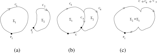
Figure 2: Composition of surfaces with the disk topology. (a) Surfaces $\Sigma_{i}$ with the marked points $P_{i}$ and the clockwise oriented boundaries $C_{i}$. (b) Surfaces are joined along the common boundary segment $C_{5}$. (c) The resulting surface $\Sigma_{2}\circ\Sigma_{1}$ with the marked point $P_{1}$ and the clockwise oriented boundary $C\circ C_{4}\circ C_{3}$.

Eq.(9) can be understood as follows. When the curve $C$ is absent, i.e. when the marked points of $\Sigma_{1}$ and $\Sigma_{2}$ coincide, eq. (9) simplifies to

$$W[\Sigma_{2}\circ\Sigma_{1}]=W[\Sigma_{2}]V[\Sigma_{2}](W[\Sigma_{1}]),$$

$$V[\Sigma_{2}\circ\Sigma_{1}]=V[\Sigma_{2}]V[\Sigma_{1}].$$ (10)

Thus when the marked points of the two surfaces coincide, the Wilson surfaces are composed as in eq. (10). If we think of $V[\Sigma,P]$ as an operator which acts on the objects with the marked point $P$ and assume that only the objects with the same marked points can be multiplied, then the meaning of eq. (9) becomes clear. The role of $M[C]$ in eq. (9) is to transform the objects with the marked point $P_{2}$ to the objects with the marked point $P_{1}$.

Figure 3: $\Sigma_{3}\circ(\Sigma_{2}\circ\Sigma_{1})\neq\Sigma_{2}\circ(\Sigma_{3}\circ\Sigma_{1})$

Composition of three or more surfaces is in general ambiguous. Consider figure 3. Using the composition rule (9) it can be shown that

$$W[\Sigma_{3}\circ(\Sigma_{2}\circ\Sigma_{1})]\neq W[\Sigma_{2}\circ(\Sigma_{3}\circ\Sigma_{1})],$$

$$V[\Sigma_{3}\circ(\Sigma_{2}\circ\Sigma_{1})]\neq V[\Sigma_{2}\circ(\Sigma_{3}\circ\Sigma_{1})].$$ (11)

Given

$$V[\delta\Sigma]\approx 1+v[P]\equiv 1+v_{\mu\nu}[P]\sigma^{\mu\nu}$$ (12)

for an infinitesimal surface $\delta\Sigma$ with the area element $\sigma^{\mu\nu}$, we want to find $V[\Sigma]$ for a finite-size surface $\Sigma$. This can be done using a trick similar to the one used in the context of the non-abelian Stokes formula [5]. Consider the contour $C^{\prime}$ in figure 4. From the relation

$$M[C^{\prime}]=M[C_{P}^{-1}]M[\delta C]M[C_{P}]M[C]$$ (13)

and eq. (7) one finds

$$V[\Sigma^{\prime}]=M[C_{P}^{-1}]V^{-1}[\delta\Sigma]M[C_{P}]V[\Sigma].$$ (14)

Thus we have

$$\delta V[\Sigma]=M[C_{P}^{-1}]v[P]M[C_{P}]V[\Sigma].$$ (15)

A solution of this equation involves a choice of ordering and it is given by

$$V[\Sigma]={\hat{P}}_{\tau}\exp\left(\int_{\Sigma}M[C_{P}^{-1}]v[P]M[C_{P}]\right),$$ (16)

where ${\hat{P}}_{\tau}$ is the ordering in $\tau$ and the curve $C_{P}$ is defined in figure 5. Note that the expression eq. (16) depends on the parametrization $x^{\mu}=x^{\mu}(\sigma,\tau)$ of the surface $\Sigma$. For example a boundary-preserving reparametrization will change $C_{P}$ to a $C^{\prime}_{P}$ (see figure 5). Thus $V[\Sigma]$ and $W[\Sigma]$ depend on the parametrization of $\Sigma$:

$$V=V[\Sigma,x^{\mu}(\sigma,\tau)],~{}~{}~{}W=W[\Sigma,x^{\mu}(\sigma,\tau)].$$ (17)

In section 3 we will see that if $(\sigma,\tau)$ and $({\tilde{\sigma}},{\tilde{\tau}})$ are two different parametrizations of a surface $\Sigma$, then

$$(V[\Sigma,x^{\mu}(\sigma,\tau)],W[\Sigma,x^{\mu}(\sigma,\tau)])$$

and

$$(V[\Sigma,x^{\mu}({\tilde{\sigma}},{\tilde{\tau}})],W[\Sigma,x^{\mu}({\tilde{\sigma}},{\tilde{\tau}})])$$

are related by the gauge transformation. In other words, the non-abelian internal symmetry and the reparametrization symmetry mix.

Figure 4: Contour $C^{\prime}=C_{P}^{-1}\circ\delta C\circ C_{P}\circ C$.

3 Gauge transformations

In this section we introduce the gauge transformations which compensate the ambiguity in the composition of NWS. Suppose that a surface $\Sigma$ is composed out of three or more smaller surfaces. Let $(W[\Sigma],V[\Sigma])$ and $({\tilde{W}}[\Sigma],{\tilde{V}}[\Sigma])$ correspond to two different compositions resulting in the surface $\Sigma$. We have

$$M[C]=i_{W[\Sigma]}V[\Sigma]=i_{{\tilde{W}}[\Sigma]}{\tilde{V}}[\Sigma].$$ (18)

Since $W$ and ${\tilde{W}}$ are elements of a group $G$, there is a group element $R[\Sigma]\in G$ such that

$${\tilde{W}}[\Sigma]=W[\Sigma](R[\Sigma])^{-1}.$$ (19)

Let us decompose $W$ and ${\tilde{W}}$ into the abelian and non-abelian factors:

$$W=W_{\scriptstyle{\rm ab}}\cdot W_{\scriptstyle{\rm nonab}},~{}~{}~{}~{}~{}{\tilde{W}}={\tilde{W}}_{\scriptstyle{\rm ab}}\cdot{\tilde{W}}_{\scriptstyle{\rm nonab}}.$$ (20)

It is clear that the ambiguity in the composition does not affect the abelian part. Thus we have

$${\tilde{W}}_{\scriptstyle{\rm ab}}[\Sigma]=W_{\scriptstyle{\rm ab}}[\Sigma].$$ (21)

Combining this equation with eq. (19) we find

$${\tilde{W}}_{\scriptstyle{\rm nonab}}[\Sigma]=W_{\scriptstyle{\rm nonab}}[\Sigma](R[\Sigma])^{-1}.$$ (22)

We propose that eq. (21) and eq. (22) define the gauge transformation of $W$. In order for this gauge transformation of $W$ to be compatible with eq. (18), $V$ should transform as

$${\tilde{V}}[\Sigma]=i_{R[\Sigma]}V[\Sigma].$$ (23)

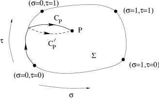
Figure 5: A parametrized surface $\Sigma$. The path $C_{P}$ consists of two segments: the first segment $(\sigma=0={\rm const.},\tau)$ is from $\tau=0$ to $\tau$ and the second segment $(\sigma,\tau={\rm const.})$ is from $\sigma=0$ to $\sigma$.

It can be checked that the gauge transformations (21–23) are compatible with the composition rule (9) provided that the composition rule for $R$ is the same as that of $W$, namely

$$R[\Sigma_{2}\circ\Sigma_{1}]=M[C](R[\Sigma_{2}])M[C]V[\Sigma_{2}]M[C^{-1}](R[\Sigma_{1}]).$$ (24)

More generally, consider a surface $\Sigma$ divided into $n$ smaller surfaces $\Sigma_{1},\ldots,\Sigma_{n}$. Let $C$ be the boundary of $\Sigma$. Repeating the reasoning leading to eq. (9) we have

$$M[C]=M[{\cal C}_{1}]i_{W[\Sigma_{1}]}V[\Sigma_{1}]M[{\cal C}_{2}]i_{W[\Sigma_{2}]}V[\Sigma_{2}]M[{\cal C}_{3}]\cdots$$ (25)

for some curves ${\cal C}_{1},{\cal C}_{2},\ldots$. From this equation we find

$$W[\Sigma]=M[{\cal C}_{1}](W[\Sigma_{1}])M[{\cal C}_{1}]V[\Sigma_{1}]M[{\cal C}_{2}](W[\Sigma_{2}])\ldots,$$

$$V[\Sigma]=M[{\cal C}_{1}]V[\Sigma_{1}]M[{\cal C}_{2}]V[\Sigma_{2}]M[{\cal C}_{3}]\ldots.$$ (26)

It is easy to see that the gauge transformations (21– 23) are compatible with eq. (26) provided that $R[\Sigma]$ is composed out of $R[\Sigma_{i}]$ as follows:

$$R[\Sigma]=M[{\cal C}_{1}](R[\Sigma_{1}])M[{\cal C}_{1}]V[\Sigma_{1}]M[{\cal C}_{2}](R[\Sigma_{2}])\ldots.$$ (27)

Thus $R$ should be composed by the rule of composition of $W$.

We now introduce new gauge transformations. These are the transformations of $M$, $V$ and $W$ compatible with eq. (7).

Let $\Lambda[P]$ be an ${\rm Aut}(G)$-valued function of point $P$. Let $C$ be a directed path from $P_{1}$ to $P_{2}$. The gauge transformation of $M[C]$ reads

$${\tilde{M}}[C]=\Lambda[P_{2}]M[C]\Lambda[P_{1}]^{-1}.$$ (28)

When $P_{1}=P_{2}=P$ this equation becomes

$${\tilde{M}}[C]=\Lambda[P]M[C]\Lambda[P]^{-1}.$$ (29)

From this equation and

$${\tilde{M}}[C]=i_{\tilde{W}}{\tilde{V}}$$ (30)

one finds

$$i_{W}V=\Lambda^{-1}i_{\tilde{W}}{\tilde{V}}\Lambda=i_{\Lambda^{-1}({\tilde{W}})}\Lambda^{-1}{\tilde{V}}\Lambda.$$ (31)

Thus we propose the gauge transformations:

$${\tilde{V}}[\Sigma,P]=\Lambda[P]V[\Sigma,P]\Lambda[P]^{-1},$$

$${\tilde{W}}[\Sigma,P]=\Lambda[P](W[\Sigma,P]).$$ (32)

We now consider a new gauge transformation which is a finite generalization of the infinitesimal transformation considered in [2]. The transformation reads

$${\tilde{M}}[C]=i_{{\cal Z}[C]}M[C],$$ (33)

where ${\cal Z}[C]$ is a $G$-valued functional of $C$. The composition rule for ${\cal Z}$ can be inferred from the following chain of equations:

$$i_{{\cal Z}[C_{2}\circ C_{1}]}M[C_{2}\circ C_{1}] = {\tilde{M}}[C_{2}\circ C_{1}]$$ (34)

$$= {\tilde{M}}[C_{2}]{\tilde{M}}[C_{1}]$$

$$= i_{{\cal Z}[C_{2}]}M[C_{2}]i_{{\cal Z}[C_{1}]}M[C_{1}]$$

$$= i_{{\cal Z}[C_{2}]}i_{M[C_{2}]({\cal Z}[C_{1}])}M[C_{2}\circ C_{1}].$$

This equation suggests the following composition rule for ${\cal Z}$:

$${\cal Z}[C_{2}\circ C_{1}]={\cal Z}[C_{2}]M[C_{2}]({\cal Z}[C_{1}]).$$ (35)

If a Lie($G$)-valued 1-form $\zeta$ is given, ${\cal Z}[C]$ for an open path $C$ can be constructed as follows. Let us divide $C$ into $n$ small subpaths as in figure 6(a). Applying eq. (35) we find

$${\cal Z}[C] = {\cal Z}[C_{n}]\cdot M[C_{n}](Z[C_{n-1}])\cdot M[C_{n}\circ C_{n-1}]({\cal Z}[C_{n-2}])\cdots$$ (36)

$$~{}~{}M[C_{n}\circ C_{n-1}\cdots C_{2}]({\cal Z}[C_{1}])$$

$$\approx (1+\zeta_{\mu}[P_{n}]dx^{\mu})(1+M[C_{n}](\zeta_{\mu}[P_{n-1}])dx^{\mu})\cdots$$

$$~{}~{}(1+M[C_{n}\circ C_{n-1}\cdots C_{2}](\zeta_{\mu}[P_{1}])dx^{\mu}).$$

In the large $n$ limit we thus find

$${\cal Z}[C]={\hat{P}}~{}{\rm exp}\left(\int_{C}M[C^{\prime\prime}](\zeta_{\mu}[P])dx^{\mu}\right),$$ (37)

where $C^{\prime\prime}$ and $P$ are as in figure 6(b), and ${\hat{P}}$ is the path ordering operator.

Figure 6: (a) The path $C$ is divided into $n$ small subpaths: $C=C_{n}\circ C_{n-1}\cdots\circ C_{1}$. (b) The point $P$ divides $C=C^{\prime\prime}\circ C^{\prime}$.

A choice of transformation of $V$ and $W$ compatible with eq. (7) and eq. (33) is

$${\tilde{V}}[\Sigma,C]=V[\Sigma,C],$$

$${\tilde{W}}[\Sigma,C]={\cal Z}[C]W[\Sigma,C].$$ (38)

Infinitesimal versions of these transformations agree with the transformations that can be derived from [2]. Let us consider an infinitesimal surface $\delta\Sigma$ with the area element $\sigma^{\mu\nu}$. Assume that $M[C]\in{\rm Aut}(G)$ is an inner automorphism given by

$$M[C](g) = {\hat{P}}{\rm exp}\left(\int_{C}\mu\right)~{}g~{}{\hat{P}}{\rm exp}\left(-\int_{C}\mu\right)$$ (39)

$$= {\hat{P}}{\rm exp}\left(\int_{C}\mu_{\scriptstyle{\rm adjoint}}\right)(g),~{}~{}~{}~{}~{}\forall g\in G,$$

where $\mu$ is a Lie($G$)-valued 1-form. From eq. (38) and

$$W[\delta\Sigma]\approx 1+B_{\mu\nu}\sigma^{\mu\nu},$$ (40)

one can find the transformation of the 2-form $B$:

$${\tilde{B}}=B+d\zeta-{1\over 2}[\zeta,\zeta]-[\mu,\zeta].$$ (41)

The transformation of $B$ corresponding to eqs.(21,22) reads

$${\tilde{B}}_{\scriptstyle{\rm ab}}=B_{\scriptstyle{\rm ab}},~{}~{}~{}~{}{\tilde{B}}_{\scriptstyle{\rm nonab}}=B_{\scriptstyle{\rm nonab}}-\rho,$$ (42)

where $\rho$ is a Lie($G$)-valued 2-form defined in

$$R[\delta\Sigma]\approx 1+\rho_{\mu\nu}\sigma^{\mu\nu}.$$ (43)

Eq.(42) agrees with the transformations that can be derived from [2].

Unlike the gauge transformations (21–23, 32), the transformation (38) is not compatible with the composition rule (9). To find the correct transformation, ${\cal Z}[C]$ in eq. (38) should be ‘smeared’ over the surface $\Sigma$. We give an explicit formula for the gauge transformation of $V[\Sigma]$. It reads

$${\tilde{V}}[\Sigma]={\hat{P}}_{\tau}\exp\left(\int_{\Sigma}i_{{\cal Z}[C_{P}]}M[C_{P}]v[P]M[C_{P}^{-1}]i_{{\cal Z}[C_{P}]^{-1}}\right).$$ (44)

4 Comments

$\bullet$ We found three kinds of gauge transformations of $M$, $V$ and $W$. These are $\Lambda[P]$-transformations (28,32), $R[\Sigma]$-transformations (21–23) and ${\cal Z}[C]$-transformations (33,38). Eq.(38) is valid only for infinitesimal surfaces and should be replaced by a ‘smeared’ version eq. (44).

$\bullet$ The ambiguity in surface-ordering necessitates the introduction of gauge transformations which compensate the ambiguity. Locally this amounts to the transformation eq. (42). The number of gauge degrees of freedom present in a NWS is enormous. Thus NWS may be relevant to a topological string theory describing topological sectors of the non-abelian string of [3].

$\bullet$ Infinitesimal version of eq. (9) can be derived from the composition rule for the natural transformation $K$ in figure 1.

$\bullet$ We defined NWS on a local trivial patch. To define NWS globally one should cover the manifold with an atlas $\{U_{\alpha}\}$ and introduce $W_{\alpha},V_{\alpha},M_{\alpha}$ for each patch $U_{\alpha}$. As usual the quantities on the overlaps $U_{\alpha\beta}=U_{\alpha}\cap U_{\beta}$ are related by the gauge transformations. An analysis of global issues will be carried out elsewhere.

$\bullet$ We defined NWS with the disk topology. A generalization to higher-genus surfaces will be discussed elsewhere.

Note added

After submitting the original version of this paper to hep-th, the work [6] was brought to our attention. In [6] an equation similar to eq. (16) was taken as a definition of Wilson surface. The case considered in [6] corresponds, in our notation, to the $C$-independent $M[C]$. The surface-ordering ambiguities are absent in this case. For a list of miscellaneous work on non-abelian 2-form theories, see [7].

Acknowledgments

This work was supported by the DOE under grant No. DE-FG03-92ER40701, by the Research Foundation under NSF grant PHY-9722101 and by CRDF Award RP1-2108.