Abstract

We discuss different dualities of QHE in the framework of the noncommutative Chern-Simons theory. First, we consider the Morita or T-duality transformation on the torus which maps the abelian noncommutative CS description of QHE on the torus into the nonabelian commutative description on the dual torus. It is argued that the Ruijsenaars integrable many-body system provides the description of the QHE with finite amount of electrons on the torus. The new IIB brane picture for the QHE is suggested and applied to Jain and generalized hierarchies. This picture naturally links 2d $\sigma$-model and 3d CS description of the QHE. All duality transformations are identified in the brane setup and can be related with the mirror symmetry and S duality. We suggest a brane interpretation of the plateu transition in IQHE in which a critical point is naturally described by $SL(2,R)$ WZW model.

1 Introduction

Non-commutative field theories (see [1] for a review and references therein)are with us since some time and they owe their raison d’être to a variety of reasons. The most recent one is string theory [2] which in a particular region of parameter space produces non-commutative field theory in very much the same way as the lowest Landau level starts to produce non-commuting coordinates in a very strong magnetic field. This phenomenon was studied in the thirties by Moyal, Peierls and many others in the setting of an additional periodic potential.

Another way of producing non commutative gauge theory occurred in the phenomenon of transmutation of internal (color) to external (space time) degrees of freedom. This was popular in the early eighties and went by the name of twisted Eguchi-Kawai models [3]. The idea was to have a sequence of conventional SU(N) gauge theories with twisted boundary conditions on a finite lattice (or even one point lattice) and to produce a NC theory on a large lattice.

The interaction between the photons in the NC theory vanishes linearly in the momenta, when they are small with respect to the NC scale $\mu$ in contrast to the ordinary YM coupling. On the other hand one can express the free energy of the NC theory in a periodic box of size $L$.L is supposed to be larger, by an integer factor N, with respect to the NC scale. Then, to all orders in perturbation theory, the free energy of NCU(1) equals the free energy of conventional SU(N) gauge theory in a twisted box. The size of this box is small with respect to the NC scale. And the coupling of the NC theory rescales by this same factor $N$. This is the simplest form of Morita duality [5].

Another raison d’être of NCU(1) theory was its connection with large N theory. In fact Gonzalez-Arroyo et al [4] showed for fixed cut-off that the non-planar sector is suppressed in the limit of infinitely large NC length scale $\mu^{-1}$, whereas the planar sector is identical. Only for exceptional momenta the non-planar sector can survive.

When the parameter of noncommutativity is rational one can map the noncommutative gauge theories to the commutative gauge theories with twisted boundary conditions. Under the Morita duality transformation in d dimensions the topological numbers of the bundles, namely the rank, flux and the Pontryagin number are transformed under SO(d,d,Z) action. The noncommutativity parameter $\theta$ gets mapped into the twist in the dual commutative YM theory. There exists an explicit mapping of the gauge fields under this transformations [9].

It was also recognized recently that noncommutative Chern-Simons theory provides the appropriate language for the description of the FQHE [6]. The particle density and the filling factor get mapped into the noncommutativity parameter and the coefficient in front of the CS action. Generalization of the picture for a finite amount of electrons having the finite extent on the plane was found in [7]. It appears that the corresponding regularized model is equivalent to the rational Calogero model with the oscillatory potential. Actually the relation between Calogero type models and FQHE was known for a while [8] however it was not exploited so far.

Therefore the natural question is if there exists a formulation of FQHE in terms of the twisted commutative gauge theory. The natural candidate for the commutative gauge description of the FQHE is commutative CS action considered in [10]. In this paper we will show how such commutative description can be formulated providing the realization of the Morita equivalence in the context of FQHE. This issue has been briefly discussed in [11]. In what follows we will consider models with a finite number of electrons since precisely in this case Morita duality can be formulated in a very explicit way. First, we consider the FQHE on the disc and map it into the model on the cylinder described by the trigonometric Calogero (Sutherland) model using the dualities known in the context of the integrable many body systems [12]. Then we use the YM formulation of the trigonometric Calogero model [13] to clarify the version of Morita equivalence in this case.

It is the degenerate case of a more general situation when the FQHE is defined on the torus and therefore there is a finite number of electrons from the very beginning. The equivalent many-body system is now the relativistic trigonometric Ruijsenaars model which is known to allow a description as a commutative CS theory on the dual torus [14]. In this case Morita duality is quite transparent.

The NCCS description of FQHE yields the IIA brane realization of the corresponding theory [15, 16] via the configuration of D0, D2 and D6(D8) branes. In the context of D branes Morita duality is nothing but T duality transformation. Therefore we shall match the brane interpretation of FQHE with the T dual realizations via the gauge theories. On the other hand we shall exploit the brane realizations of the integrable systems known in the context of SUSY gauge theories (see [17] for a review and references therein). In this paper we suggest new IIB type description for the FQHE in terms of D1, D3, and 5 branes based on the known realization of the CS term in IIB type theory [18]. We develop the IIB brane picture for Jain and generalized hierarchies.

Besides the T duality transformation mapping between two equivalent description of the given QH system there are additional duality which are consistent with RG flows between the members of the whole FQHE family. These duality transformations constitute the infinite discrete group $\Gamma_{U}(2)$ and impose the restriction on the $\beta$ function in the theory. Using the IIB picture we identify all basic transforms from the duality group in the brane terms. Moreover we conjecture the brane interpretation of the RG transitions between the plateaux as the motion of D3 branes in the five branes web. This conjecture appears to be in the rough agreement with the existence of the critical point between two plateaux.

Let us emphasize that we have branes of different dimensions involved in our configuration. Therefore any physical phenomena concerning the Quantum Hall system looks differently from the point of view of the gauge theories defined on the worldvolumes of D1, D3 or (p,q) 5 branes. Namely, from D1’s point of view one deals with the $\sigma$ model on the complicated manifold determined by the brane configuration. From the point of view of the theory on D3’s we will consider the pure Chern-Simons theory or Maxwell Lagrangian with CS term. Finally, theory defined on the five branes provides the d=6 or d=5 theory where some defects, for instance monopole like configurations, are represented by D1 and D3 branes.

The paper is organized as follows. In Section 2 we describe the realization of the FQHE on the disc in terms of the commutative YM on the cylinder with inserted Wilson line. In Section 3 we consider the Morita dual description of FQHE on the torus using the formulation of the model with the finite amount of electrons in terms of the Ruijsenaars integrable many-body system. In Section 4 we consider duality transformations relevant to the RG behavior of the FQHE systems and compare them with the dualities known in the context of the Calogero-Ruijsenaars type models. Section 5 is devoted to the new IIB brane picture which is applied for the Jain and generalized hierarchies. In Section 6 we identify transformations from the duality group $\Gamma_{0}(2)$ of the RG flows as well as the particle-hole symmetry in the brane terms. The picture of RG flows between the two plateaux in the brane terms is conjectured. Section 7 contains some conclusions and speculations.

2 U(1) NCCS and YM on the cylinder

2.1 The Chern-Simons matrix model

The starting point of our considerations is the realization of U(1) NCCS theory via infinite matrixes $X_{a}$ [6]

$$S=\int dtBTr\{\epsilon_{ab}(\dot{X_{a}}+i[A_{0},X_{a}])X_{b}+2\theta A_{0}\}$$ (1)

where the trace over the Hilbert space substitutes the integration over the noncommutative plane in the matrix formulation. The averaged density of electrons is

$$\rho=\frac{2\pi}{\theta}$$ (2)

The coefficient in front of the CS action is related to the filling fraction $\nu$ as follows

$$k=\frac{B\theta}{4\pi}=\frac{1}{4\nu}$$ (3)

The action enjoys gauge invariance and the Gauss law constraint supports the noncommutativity of the coordinates

$$[X_{1},X_{2}]=i\theta$$ (4)

To consider the model with a finite number of electrons it was suggested to use the finite gauged matrix model [22]

$$S=\int dtBTr\{\epsilon_{ab}(\dot{X_{a}}+i[A_{0},X_{a}])X_{b}+2\theta A_{0}-BX_{a}^{2}\}+\Psi^{+}(i\dot{\Psi}-A_{0}\Psi)$$ (5)

where coordinates are represented now by $N\times N$ matrixes. The additional fields $\Psi$ which are necessary to be introduced take care of the boundary of the droplet and transform in the fundamental of the gauge group U(N). The density of the electrons in the model $\rho=\frac{N}{\pi R^{2}}$ coincides with the infinite case since the radius of the droplet is of order $\sqrt{N\theta}$.The excitations of the finite model perfectly match the excitations known in the FQHE [23].

It can be shown that after the resolution of the Gauss law constraint the matrix model becomes equivalent to the rational Calogero model

$$H=\sum_{n=1}^{N}(1/2p_{n}^{2}+1/2B^{2}X_{n}^{2})+\sum_{n\neq m}\frac{\nu^{-2}}{(x_{n}-x_{m})^{2}}$$ (6)

The positions of the Calogero particles are the eigenvalues of $X_{1}$ while momenta can be identified with the diagonal elements of $X_{2}$. Since the Hamiltonian of the Calogero model coincides with the potential in the matrix model the states map between the two models. In what follows we shall use the mapping to the many-body systems to formulate the commutative gauge theory.

2.2 Mapping to the trigonometric Calogero model

To get the link with the gauge theory let us describe at the first step the map of the model above into the Sutherland model with the Hamiltonian representing a system of indistinguishable particles on a circle $S^{1}_{R}$ of the radius $R$, interacting with the pair-wise potential [21]

$$U_{suth}(q)={{{\xi}^{2}}\over{4R^{2}{\sin}^{2}({{q}\over{2R}})}}$$ (7)

This is a simple example of the dualities between the pairs of the integrable many-body systems [12] which can be effectively described in terms of the Hamiltonian reduction procedure.

From the Hamiltonian point of view the system has the phase space:

$$M_{suth}=[T^{*}\bigl{(}S^{1}_{R}\bigr{)}^{N}]/{S}_{N}$$ (8)

where $S_{N}$ is the $N$-th order symmetric group. The coordinates in the phase space will be denoted as $(p_{i},q_{i})$ where $q_{i}$ is the angular coordinate on the circle $S^{1}_{R}$ and $p_{i}$ is the corresponding momentum. The Hamiltonian of the many-body system $H_{suth}$ has the natural form:

$$H_{suth}=\sum_{i=1}^{N}{{p_{i}^{2}}\over{2}}+\sum_{i\neq j}U_{suth}(q_{i}-q_{j})$$ (9)

which is a well-known Sutherland model (see [20] for the review on the Calogero-Sutherland models).

We shall present now the explicit map between the Sutherland model and the Hamiltonian (6) providing the description of the FQHE on the disc. The phase space of the rational model is

$$M_{cal}=[T^{*}{R}^{N}]/{S}_{N}$$ (10)

Hereafter we will extensively use the group like description of the Calogero type models. The most effective approach appears to be the Hamiltonian reduction procedure.

Recall how the Hamiltonian reduction gives rise to the systems discussed. The main idea behind the construction is to realize the (classical) motion due to the Hamiltonians as a projection of the simple motion on a somewhat larger phase space. In the Sutherland case one starts with the symplectic manifold $X_{suth}=T^{*}G\times{C}^{N}$ where $G=U(N)$ with the canonical Liouville form

$$\Omega_{suth}=iTr\delta(p\wedge\delta gg^{-1})+{1\over{2i}}\delta v^{+}\wedge\delta v$$ (11)

Here $p$ represents the cotangent vector to the group $G$. We think of it as of the Hermitian matrix. The manifold $X_{suth}$ is acted on by $G$ by conjugation on the $T^{*}G$ factor and in a standard way on $C^{N}$. The action is Hamiltonian with the moment map:

$$\mu_{suth}=p-g^{-1}pg-v\otimes v^{+}$$ (12)

One performs the reduction at the level of the moment map and takes its quotient by $G$. Explicitly, one solves the equation

$$p-g^{-1}pg-v\otimes v^{+}=-\xi 1$$ (13)

up to the $G$-action. The way to do it is to fix a gauge

$$g={\exp}({i\over{R}}diag(q_{1},\ldots,q_{N}))$$

and then solve for $p$ and $v$. One has:

$$v_{i}={\sqrt{\xi}},\quad p_{ij}=Rp_{i}\delta_{ij}+{\xi}{{1-{\delta}_{ij}}\over{e^{{i(q_{i}-q_{j})}\over{R}}-1}}$$

As a result one gets the reduced phase space:

$$M_{suth}=[T^{*}(S^{1})^{N}]/S_{N}$$ (14)

with the canonical symplectic structure

$$\Omega_{suth}^{red}=\sum_{i}\delta p_{i}\wedge\delta q_{i}$$

The complete set of functionally independent integrals is given by:

$$H_{suth}^{(k)}={1\over{R^{k+1}}}Trp^{k+1},\qquad k=0,\dots,N-1$$ (15)

The unreduced phase space of the rational Calogero system has the form $X_{cal}=T^{*}g\times C^{N}$ where $g=LieU(N)$. The group acts on this manifold and upon the reduction on the level of the moment map one obtains the reduced phase space mentioned above.The set of independent Hamiltonians in the rational model amounts from

$$H^{k+1}=Tr(ZZ^{+})^{k+1}$$ (16)

where $Z=P+iQ,(P,Q)\in LieU(N)$.

The symplectic map between two models looks as follows. First, elements from $C^{N}$ get unchanged, coupling constants in two models coincide while the map sends Z to the polar decomposition

$$Z=\sqrt{Bp}g$$ (17)

where p is supposed to be hermitian matrix with the non-negative eigenvalues. The frequency of the oscillator in the rational model gets mapped into the radius in the Sutherland model

$$B=R^{-1}$$ (18)

and the quadratic Hamiltonian of the Calogero model is mapped to the total momentum of the Sutherland model. Higher hamiltonians are mapped as well, for instance quadratic Hamiltonian of the Sutherland model is mapped in the quartic Hamiltonian in the Calogero system. This correspondence survives at the quantum level and the spectrum of the Hamiltonian of the Calogero model exactly coincides with the spectrum of the total momentum in the Sutherland model.

2.3 Sutherland system from 2D YM theory

Let us show how the Lagrangian formulation of the Sutherland systems amounts from the YM theory on the cylinder [13]. Consider the central extension of the loop algebra ${\cal L}G$, where $G$ is a semisimple Lie algebra. We take the cotangent bundle to the algebra as a bare phase space, namely $(A,k;\phi,c)$, where $\phi$ - $G$ - valued scalar field , $c$ - the central element , $A$ - the gauge field on the circle and $k$ - is dual to $c$. A natural symplectic structure is defined as follows

$$\Omega=\int Tr(\delta\phi\wedge\delta A)+\delta c\wedge\delta{\kappa}$$ (19)

while the adjoint and coadjoint action of the loop group ${\cal L}G$ on $\hat{g}$ and ${\hat{g}}^{*}$ reads

$$(\phi(\varphi),c)\rightarrow(g(\varphi)\phi(\varphi)g(\varphi)^{-1},\int Tr(-\phi g^{-1}{\partial_{\varphi}}g)+c)$$ (20)

$$(A,{\kappa})\rightarrow(gAg^{-1}+{\kappa}g{\partial_{\varphi}}g^{-1},{\kappa})$$ (21)

This action clearly preserves the symplectic structure and thus defines a moment map

$$\mu:T^{*}{\hat{g}}\rightarrow{\hat{g}}^{*},$$

which takes $(\phi,c;A,{\kappa})$ to $({\kappa}d\phi+[A,\phi],0)$.

Let us remind that the choice of the level of the moment map has a simple physical meaning - in the theory of the angular momentum just the sector of the Hilbert space is fixed. In the gauge theory one selects the gauge invariant states. It is natural to consider an element $J$ from $g^{*}$, which has the maximal stabilizer different from the whole $G$. It is easy to show that the representative of the coadjoint orbit of this element has the following form

$$J_{\nu}={\nu}\sum_{\alpha\in\Delta_{+}}(e_{\alpha}+e_{-\alpha}),$$ (22)

where $\nu$ is some real number, $e_{\pm\alpha}$ are the elements of nilpotent subalgebras $n_{\pm}\subset g$, corresponding to the roots $\alpha$, and ${\Delta}_{+}$ is the set of positive roots. Let us denote the orbit of $J_{\nu}$ as ${\cal O}_{\nu}$. When quantizing ${\cal O}_{\nu}$ we get a $R_{\nu}$ representation of $G$. For generic $J\in g^{*}$ denote as $G_{J}$ the stabilizer $J$ of the orbit ${\cal O}_{J}$, that is ${\cal O}_{J}=G/G_{J}$. Therefore the proper orbit in the affine case ${\cal O}_{\nu}$

$$\mu=({\cal J}[{\mu}],0):{\cal J}[{\mu}]({\varphi})=\delta({\varphi})J_{\nu}$$ (23)

is finite dimensional.

To perform a reduction one has to resolve the moment map which has the meaning of a Gauss law in the affine case

$${\kappa}\partial_{\varphi}\phi+[A,\phi]=J_{\mu}({\varphi})=\delta({\varphi})J_{\nu}.$$ (24)

It is useful to resolve the constraint in the following manner. First, we use the generic gauge transformation $\tilde{g}({\varphi})$ to make $A$ to be a Cartan subalgebra valued one form $D$. We are left with the freedom to use the constant gauge transformations which do not affect $D$. Actually the choice of $D$ is not unique and is parameterized by the conjugacy classes of monodromy $\exp(\frac{2\pi}{\kappa}D)\in{\bf T}\subset G$. Let us fix the conjugacy class denoting as ${\sf i}x_{i}$ the elements of the matrix $D=iX$. Let us decompose the $g$ - valued function $\phi$ on the $S^{1}$ on Cartan $P(\varphi)\in t$ and nilpotent ${\phi}_{\pm}({\varphi})\in n_{\pm}$ components. Let ${\phi}_{\alpha}=<{\phi},e_{\alpha}>$, then (24) reads:

$${\kappa}\partial_{\varphi}P=\delta({\varphi})[J_{\nu}^{g}]_{\gamma}$$ (25)

$${\kappa}\partial_{\varphi}{\phi}_{\alpha}+<D,{\phi}_{\alpha}>=\delta({\varphi}){[J_{\nu}^{g}]}_{\alpha},\\$$ (26)

where $J_{\nu}^{\tilde{g}}$ - $Ad_{{\tilde{g}}(0)}^{*}(J_{\nu})$, $[J]_{\gamma}$ denotes the Cartan part of $J$ and $[J]_{\alpha}=<J,e_{\alpha}>$.

From (25) one gets $D=constant$ and $[J_{\nu}^{g}]_{\gamma}=0$. Therefore we can twist back $J^{g}_{\nu}$ to $J_{\nu}$ . Moreover, (26) implies, that (if $\varphi\neq 0$ ) can be presented ${\phi}_{\alpha}({\varphi})$ in the following form:

$${\phi}_{\alpha}({\varphi})=\exp(-\frac{\varphi}{\kappa}<D,{\alpha}>)\times M_{\alpha},$$ (27)

where $M_{\alpha}$ is locally constant element in $g$. It is evident that $M_{\alpha}$ jumps, when ${\varphi}$ goes through $0$. The jump is equal to

$$[\exp(-\frac{2\pi}{\kappa}<D,{\alpha}>)-1]\times M_{\alpha}=[J^{g}_{\nu}]_{\alpha}.$$ (28)

Finally the physical degrees of freedom are $\exp(-\frac{2\pi i}{\kappa}X)$ and $P$ with the symplectic structure

$$\omega=\frac{1}{2\pi i}Tr(\delta P\wedge\delta X)$$ (29)

and

$${\phi}_{\alpha}({\varphi})={\xi}\frac{\exp(-\frac{i\varphi}{\kappa}<X,{\alpha}>)}{\exp(-\frac{2\pi i}{\kappa}<X,{\alpha}>)-1}.$$

Collecting together the term yielding the Poisson structure moment map with the lagrangian multiplier $A_{0}$ and the second Casimir

$${\cal H}_{2}=\frac{1}{4\pi}\int_{S^{1}}d{\varphi}<{\phi},{\phi}>,$$ (30)

we immediately recognize the 2d YM theory in the hamiltonian formulation with the additional Wilson line included. On the reduced manifold we obtain the Sutherland system with the hamiltonian

$$H_{2}=-\frac{1}{2}TrP^{2}+\sum_{\alpha\in\Delta_{+}}\frac{{\xi}^{2}}{sin^{2}<X,{\alpha}>},$$ (31)

where $\Delta_{+}$ denotes the positive roots of the group $g$. For instance for $G=SU(N)$ we get the hamiltonian with the pairwise interaction

$$V_{ij}^{A}=\frac{\xi^{2}}{sin^{2}(x_{i}-x_{j})}$$

Summarizing: in this Section we presented the two step map of U(1) NCCS theory on the disc into the commutative SU(N) YM theory on the cylinder with inserted Wilson line yielding the degenerate version of the Morita duality. One should not be confused that $D=3$ CS theory is related to $D=2$ YM theory on the cylinder. The point is that YM theory on the cylinder can be derived from the G/G gauge $\sigma$ model or equivalently CS theory in the limit of large level k. On the other hand since one of the radii of the torus where CS is defined on is $R\propto k^{-1}$ the limit of large k corresponds to the theory in one dimension less. This will be more clear in the next section where the relation to the Ruijsenaars model will be discussed.

3 Ruijsenaars model and NCCS theory on the torus

In this section we will generalize the Sutherland model to the so called trigonometric Ruijsenaars model and will argue that this model provides the finite dimensional counterpart for the FQHE on the torus. Naively on the torus both momenta and coordinates have to be periodic and precisely Ruijsenaars model yields the appropriate phase space. It will be shown that this dynamical system has the moduli space of the flat connections on the torus with one marked point as phase space and the relation coming from the fundamental group gets mapped into the noncommutativity relation between coordinates on the dual torus. The rank of the gauge group G will coincide with the number of electrons in the FQHE.

In the Hamiltonian reduction approach we start with the cotangent bundle to the loop group [14] $\hat{G}$. $(g:S^{1}\rightarrow G,c\in U(1);A\in\Omega^{1}(S^{1})\otimes g^{*},{\kappa}\in{\bf R})$. The group acts as

$$g\rightarrow hgh^{-1},\;A\rightarrow hAh^{-1}+{\kappa}h{\partial}h^{-1}$$

The generalization of the Gauss law is

$$\mu(g,c;A,\kappa)=(gAg^{-1}+{\kappa}g{\partial}g^{-1}-A,0).$$ (32)

The level of the moment map looks as follows

$$\mu(g,c;A,{\kappa})={\sf i}\nu(\frac{1}{N}Id-e\otimes e^{+})\delta(\varphi).$$ (33)

As before, a general gauge transformation can be used to reduce $A$ to the diagonal form $D$ modulo the affine Weyl group action.

The moment map now becomes

$$gDg^{-1}+{\kappa}gdg^{-1}-D={\sf i}\nu(\frac{1}{N}Id-f\otimes f^{+})\delta(\varphi)$$ (34)

where $f$ - vector with the unit norm $<f,f>=1$. $f\in{\bf R}^{N}$,

$$g=\exp(\frac{\varphi}{\kappa}D)G(\varphi)\exp(-\frac{\varphi}{\kappa}D);\partial_{\varphi}G=-\frac{J}{\kappa}G\delta(\varphi),$$

where $J={\sf i}\xi(\frac{1}{N}Id-f\otimes f^{+})$. It is useful to introduce the monodromy of the connection $D$: $Z=\exp(-\frac{2\pi}{\kappa}D)=diag(z_{1},\dots,z_{N})$, $\prod_{i}z_{i}=1$, $z_{i}=\exp(\frac{2{\pi}iq_{i}}{\kappa})$ with the boundary condition:

$${\tilde{G}}^{-1}Z{\tilde{G}}=\exp(\frac{2\pi J}{\kappa})Z$$ (35)

${\tilde{G}}=G(+0)$.

The solution to the equation can be written in terms of the characteristic polynomial $P(z)$ of the matrix $Z$, ;

$$P(z)=\prod_{i}(z-z_{i}).$$

Let

$$Q^{\pm}(z)=\frac{P({\lambda}^{\pm 1}z)-P(z)}{({\lambda}^{\pm N}-1)zP^{\prime}(z)},$$

where $\lambda=e^{\frac{2\pi i\nu}{N\kappa}}$ .Then if $\lambda\to 1$, rational functions $Q^{\pm}(z)$ tend to $\frac{1}{N}$. In this notations $\tilde{G}$ looks as:

$${\tilde{G}}_{ij}=-\lambda^{-\frac{N-1}{2}}\frac{{\lambda}^{-N}-1}{{\lambda}^{-1}z_{i}-z_{j}}e^{i\theta_{i}}(Q^{+}(z_{i})Q^{-}(z_{j}))^{1/2}$$ (36)

$$=e^{i\theta_{i}-\frac{\pi i}{\kappa}(q_{i}+q_{j})}\frac{sin(\frac{\pi\nu}{\kappa})}{sin(\frac{\pi(q_{ij}-\frac{\nu}{N}}{\kappa})}\prod_{k\neq i,l\neq j}\frac{sin(\frac{\pi{q_{ik}+\frac{\nu}{N}}}{\kappa})}{sin(\frac{{\pi}q_{ik}}{\kappa})}\frac{sin(\frac{{\pi}{q_{il}-\frac{\nu}{N}}}{\kappa})}{sin(\frac{{\pi}q_{il}}{\kappa})}$$

where $\theta_{i}$ can be identified with the momenta of particles with coordinates $q_{i}$. the reduced symplectic structure is $\sim\sum_{i}d\theta_{i}\wedge dq_{i}$.

The natural gauge invariant Hamiltonian is

$$H_{\chi}=\int d{\varphi}{\chi}(g).$$

$$H_{\pm}=\sum_{i}(e^{i\theta_{i}}{\pm}e^{-i\theta_{i}})\prod_{j\neq i}f(q_{ij})$$ (37)

with the function $f(q)$:

$$f^{2}(q)=[1-\frac{sin^{2}({\pi}{\nu}/{\kappa}N)}{sin^{2}({\pi}q/{\kappa})}],$$

which yields the Ruijsenaars model , while in the limit $\kappa\to\infty$ we return back to the Sutherland one.

To fix the corresponding gauge theory we take $\int pdq$ and add the moment map equation as a constraint. The resulting action is nothing but the action of the $G/G$ sigma model with the Wilson line included [14]. The equivalent representation involves Chern-Simons theory on $X=I\times T^{2}$ with the action:

$$S_{CS}=\frac{i{\kappa}}{4\pi}\int_{X}Tr(A\wedge dA+\frac{2}{3}A\wedge A\wedge A).$$ (38)

The phase space now is the moduli space of the flat connections on the torus with the marked point where the peculiar coadjoint orbit is inserted. The latter modifies the path integral as

$$DA<v_{1}|T_{R}(P\exp\int A)|v_{2}>\exp(-S_{CS}(A)).$$

The monodromy around the marked point $U$ is specified by the highest weight $\hat{h}$ of the representation $R_{\nu}$ as $U=\exp(\frac{2\pi{\sf i}}{{\kappa}+N}\mbox{diag}({\hat{h}}_{i}))$.

Let $g_{A},g_{B}$ be the monodromies around the cycles on $T^{2}$, and $g_{C}$ the monodromy around the marked point.Then the monodromy condition on $T^{2}$ is:

$$g_{A}g_{B}g_{A}^{-1}g_{B}^{-1}=g_{C}$$

This relation becomes the condition of the noncommutativity of the coordinates on the dual torus. It can be considered as generalization of the noncommutativity relation previously discussed in the FQHE context on the disc and on the cylinder.

The natural gauge invariant Hamiltonian $cos(\frac{2\pi{\sf i}}{{\kappa}+N}{\partial}_{q})$ amounts to the difference operator with the spectrum $e^{2{\pi}{\sf i}nq}$

$$E_{n}=cos(\frac{2\pi n}{{\kappa}+N}).$$

The spectrum reads

$$\sum_{i}E_{n_{i}},$$

where we use the invariance $E_{n}=E_{n+{\kappa}+N}$ and symmetry:

$$({\kappa}+N)>n_{N}>\dots>n_{i}>\dots>n_{1}\geq 0$$ (39)

$$\sum_{i}n_{i}<({\kappa}+N)$$ (40)

It would be important to compare the excitation spectra in the Ruijsenaars model and the FQHE on the torus.

Now we are ready to formulate the Morita duality in the context of FQHE. Morita duality acts on the gauge bundle on the torus as SO(2,2,Z) transformation [5]. Generically it maps the nonabelian gauge field on the noncommutative torus $T^{2}_{\theta}$ to the abelian or nonabelian field on the dual torus $T^{2}_{\tilde{\theta}}$. The parameters of noncommutativity are related by the SO(2,2,Z) transformation

$$\tilde{\theta}=\frac{a+b\theta}{c-d\theta}$$ (41)

The rank of the gauge group as well as the flux $\int F=m$ get transformed under the duality and we shall be interested in the transformation which brings the abelian noncommutative bundle to the twisted nonabelian one. Note that the Morita duality is nothing but the T duality transform in the stringy context.

Under the duality transformation the rank and the flux get interchanged therefore starting with U(1) noncommutative theory we end with U(N) twisted abelian bundle on the dual torus where N is the number of electrons. It is necessary to check what happens with the level k in the CS action. It was shown in [11] that the effective level in CS action doesn’t change under the Morita transformation. Using this fact and the consideration above we conclude that two T dual descriptions of FQHE fit perfectly.

4 Duality in FQHE and in Calogero type systems

4.1 Dualities in FQHE

In this section we discuss the dualities known in the context of the Quantum Hall Effect and compare them with the dualities in the Calogero-Ruijsenaars type model as well with dualities in the context of supersymmetric gauge theories. In the previous section we considered the Morita duality which is the T duality transformation. It can be used in a given QH system and corresponds to two equivalent descriptions of this particular system.

The key difference with the T duality transformation which can be applied to a given system is that other dualities can be naturally applied to the whole bundle of the QHE systems over the parameter space. More exactly these symmetries can be considered as the symmetries of the RG flows between the FQHE platoeaux. To formulate these symmetries qualitatively it was suggested that the discrete group acts on the complexified conductivity [24]

$$\sigma=\sigma_{xy}+i\sigma_{xx}$$ (42)

The basic transformations which yield the duality group are the Landau level addition (L);

$$\sigma_{xy}(\nu+1)\rightarrow\sigma_{xy}(\nu)+1\qquad\sigma_{xx}(\nu+1)\rightarrow\sigma_{xx}(\nu)$$ (43)

the flux attachment transformation(F);

$$\sigma^{-1}_{xy}(\frac{\nu}{2\nu+1})\rightarrow\sigma^{-1}_{xy}(\nu)+2\qquad\sigma_{xx}(\frac{\nu}{2\nu+1})\rightarrow\sigma_{xx}(\nu)$$ (44)

and the particle-hole transformation

$$\sigma_{xy}(1-\nu)\rightarrow 1-\sigma_{xy}(\nu)\qquad\sigma_{xx}(1-\nu)\rightarrow\sigma_{xx}(\nu).$$ (45)

On the plateaux these transformations can be expressed purely in terms of the filling factors since there $\sigma_{xx}=0$. The powers of the transformations L and F amount to the discrete group of the infinite order $\Gamma_{U}(2)$. It also appeared that the particle-hole symmetry which is the outer automorphism of the $\Gamma_{U}(2)$ group amounts to the additional constraints on the structure of the RG flows [25]. The typical parameter of the RG flow could be the external magnetic field.

Using the different elements from the duality group one could generate arbitrary QH state from some fixed one. For instance, starting from $\sigma=1$ one could obtain the integer QH states with $\sigma=m$ by the transformation $L^{m-1}$, the Laughlin states $\sigma=\frac{1}{2m+1}$ by the action of $F^{m}$ and the Jain states $\sigma=\frac{p}{2mp+1}$ by the action $F^{m}L^{p-1}$.

Many properties of the QHE system just follows from the consistency of the RG flows with the duality group. For instance the semi-circle law [26], universality of the transition conductivities as well as selection rules for the transitions between plateaux [27] follow from the duality property. The universal critical points which map to themselves under the duality group are predicted. These points are located at $2\sigma_{crit}=1+i$ and their images under the duality group. The duality group, for instance, predicts that the transition between Hall plateaux with the fractions $p_{1}/q_{1}$ and $p_{2}/q_{2}$ is possible only if

$$|p_{1}q_{2}-p_{2}q_{1}|=1.$$

The discrete group provides some prediction concerning the complex $\beta$ function of the theory. It can be proven [30] that the $\beta$ function of the theory introduced in [28] should obey the following equation

$$\beta(\gamma(\sigma),\gamma(\bar{\sigma}))=\frac{\beta(\sigma,\bar{\sigma})}{(c\sigma+d)^{2}}$$ (46)

where

$$\gamma(\sigma)=\frac{a\sigma+b}{c\sigma+d}$$ (47)

with even c and $ad-bc=1$. It is also known that in the weak coupling regime the $\beta$ function behaves as

$$\frac{d\sigma}{dlogL}=-\frac{i}{2\pi Im\sigma}+higher\ loops+instanton\ contribution$$ (48)

Let us discuss now the analogies with the duality group known in the context of SUSY YM theories. First, in our opinion the analogy with N=2 SUSY theories sometimes mentioned in the literature is incorrect. The point is that the N=2 SUSY YM, contrary to FQHE, enjoys the huge moduli space therefore we could connect the nontrivial RG flows along the moduli space with the duality group in a given theory. The coordinate on the moduli space provides some RG scale and one could investigate the dependence on this coordinate.

The proper SUSY system to compare with is the N=1 theory which has no moduli space unless the fundamental matter is introduced. This theory similar to the QHE case has all loop contributions to the $\beta$ function nevertheless at least perturbatively it can be calculated exactly [32]. As for the duality group the relevant duality is the one of the RG flows between the theories with the different $N_{c},N_{f}$. The famous Seiberg duality [31] between the $SU(N_{c})$ theory with $N_{f}$ flavors and $SU(N_{f}-N_{c})$ with $N_{f}$ flavors and additional superpotential is the most elaborated example. The mirror symmetry is its d=3 counterpart. We will return to this analogy when the IIB brane picture for FQHE will be considered.

4.2 On dualities in Calogero type systems

Since the Calogero system describes the FQHE for a finite number of electrons it is reasonable to look for the map between the duality known in Calogero context to the one in FQHE. The first symmetry to be discussed is the mapping of the Calogero coupling constant $\nu$ to $\nu^{-1}$ [33]. Since the coupling constant $\nu$ in the noncommutative U(N) CS formulation is $N/k$ where N is the rank of the gauge group and k is the level, the duality is the version of rank-level duality. It can be also treated as a version of 3d mirror transformation [34].

To discuss the duality property let us proceed as follows. Let us represent the trigonometric Calogero Hamiltonian in terms of the creation-annihilation operators

$$H=\sum_{n}((1-\nu)na_{n}^{+}a_{n}+\nu Na_{n}^{+}a_{n})+\sum_{mn}(\nu a_{m}^{+}a_{n}^{+}a_{n+m}+a_{m+n}^{+}a_{m}^{+}a_{n})$$ (49)

To get the dual picture introduce new variables $\nu b_{n}^{+}=-a_{n}^{+}$ and $b_{n}=-\nu a_{n}$. The Hamiltonian in terms of the new variables is identical to the previous one upon $\nu$ gets substituted by $\nu^{-1}$ and N by -$\nu N$. The duality actually maps quasiparticles to quasiholes in the spectrum of excitations. The mapping of the coupling constant reflects the fact that the k quasiparticles have the opposite flux to the k$\nu$ quasiholes.

One more duality has a rather simple manifestation. At the quantum level the Calogero Hamiltonian depends only on the product g(1-g) where the Calogero coupling was identified with the inversed filling factor. Therefore the evident duality $g\rightarrow 1-g$ corresponds the transformation $\nu^{-1}\rightarrow 1-\nu^{-1}$.

It is known that the Calogero-Toda type systems also are relevant for the exact Seiberg-Witten solution to N=2 theory (see [17] and the references therein). Namely the periodical Toda lattice governs the nonperturbative dynamics in the pure N=2 SUSY gauge theory while the elliptic Calogero system provides the exact solution to the N=2 theory with the massive adjoint hypermultiplet. However as we have mentioned above the analogy with N=1 theories is more relevant. The relation of Calogero system to N=1 theory looks as follows. Now only the static configurations of the integrable many-body systems are relevant and they are mapped to the vacuum states of N=1 theories. One more remark is in order here. The point is that the coupling constant g of Calogero system (actually its Toda limit) can be identified with $\Lambda_{QCD}$ scale. From this point of view the duality $g\rightarrow g^{-1}$ is mapped into the relation $\Lambda_{QCD}\rightarrow\Lambda^{-1}_{QCD}$. The situation strongly resembles the relation between the nonperturbative scales in the Seiberg dual electric-magnetic pair

$$\Lambda_{el}\Lambda_{magn}=const.$$

The similarities between the RG behavior of the N=1 SUSY theories and FQHE and the role playing the Calogero type systems for both of them could provide the additional insights on the problem. Although the theories are essentially different they could manifest similar universality classes with respect to the RG flows. This relation also implies the existence of the many-body system counterpart of the S-duality known in SYM context. This problem was questioned in [12] where it was shown that S duality acts on the spectral curve of the integrable system as the modular transformation. Therefore from this point of view it is necessary to recognize the spectral curve of the corresponding integrable system in the FQHE. However since we have discussed only trigonometric models the whole machinery of S duality can not be used here. Nevertheless in what follows we have found some interpretation of S-duality transformations in the IIB brane picture and the brane interpretation of the RG will be conjectured.

5 Brane picture

5.1 IIA picture

Let us turn to the brane description of FQHE. Below we briefly review the IIA picture for the Quantum Hall system considered in [15, 16, 19].

IIA picture for FQHE according to [15, 16] looks as follows. In the picture of Susskind et.al. one considers the D2 brane in the background of k D6 branes to get the filling factor $\nu=k^{-1}$. The WZ terms in the D2 brane amount to the CS action at the level k on D2 worldvolume. Therefore the natural gauge theory on the D2 worldvolume is the Chern-Simons-Maxwell one. Since in d=3 the YM coupling constant is dimensionful it can be removed by the appropriate scaling limit. The noncommutativity in the remaining CS action follows from the D0 branes. Electrons are represented by the ends of the strings connecting D6 branes and the D2 brane.

A more elaborate picture was obtained in [16] where the system of D2 and D8 branes is considered in the massive IIA theory in the constant B field background. The CS term is induced on D2 branes due to the D8 branes. The point is that in the massive IIA theory in the NS B field background the RR rank-two field is generated as well and plays the role of the magnetic field. In the B field the nontrivial density of D6 branes on k D8 branes $\rho_{6}\propto kB$ is induced as well as density of D0 $\rho_{0}\propto NB$ on N D2 branes. The filling fraction in this case is $\nu=Nk^{-1}$. Now electrons are represented by D0 branes while the ends of the strings connecting D2 and D6 branes play the role of quasiparticles. It is known that in the massive IIA theory a fundamental string ending on any D brane carries 1/k units of the D0 charge which is consistent with QHE picture.

Let us explain how the Morita or T duality looks in IIA brane picture. Following [16] we consider one D2 brane wrapped around the torus, N D0 branes localized on the torus and representing the electrons and D8 branes generating the Chern-Simons term $k_{nc}$ on D2 worldvolume. According to the general rules the noncommutativity can be read off from the brane picture

$$\frac{\theta}{Vol}=\frac{N_{D2}}{N_{D0}}$$ (50)

and fits perfectly with identification as the inverse density of electrons. Since in this description we consider the gauge theory on the single D2 worldvolume the theory is abelian.

After the T duality transformation along the torus D2 and D0 get interchanged and we obtain the nonabelian U(N) theory on the dual torus with the unit D0 charge. Now dimensionless $\theta$ is integer and has to be treated as the twist. Finally the T duality transformation applied to D8 branes amounts to D6 branes and the corresponding strings connecting D6 and D2 branes induce $k_{c}$ on worldvolume of N D2 branes.

There was an attempt to recognize the Jain and generalized hierarchies in the IIA picture [19]. In the Jain hierarchy the effective pinning of flux to the electrons corresponds to the bound state of the D0 branes on D2 brane with 2m fundamental strings. Such composites renormalize the magnetic field and the resulting picture for the composite objects corresponds to the integer QHE. The second integer p corresponds to the number of D2 branes since it provides the rank of the group. More general hierarchies involve more general configuration of D6 branes.

5.2 IIB picture

Let us suggest a new IIB interpretation of brane configuration for FQHE. The key point we are going to exploit is the IIB interpretation of CS term [18]. To this aim consider the system of N D3 branes with worldvolume coordinates $(0126)$ stretched between NS5 brane with coordinates $(012345)$ and a (p,q) 5 brane with the same worldvolume coordinates. Note that both types of 5 branes can be derived from the M5 brane in M theory assuming the torus topology for two coordinates, say $x_{2},x_{10}$. In the IIB case NS5 branes amount from M5 brane with $(012345)$ worldvolume while (p,q) branes amount from the M5 brane wrapping $x_{2}$ coordinate q times and $x_{10}$ coordinate p times. It is also known that D3 branes come from the M2 branes in M theory picture. We shall assume that D3 branes are stretched between 5 branes separated by a distance $L_{6}$ in $x_{6}$ coordinate. The YM coupling constant in the gauge theory on D3 branes is defined as

$$\frac{1}{g_{YM}^{2}}=\frac{L_{6}}{g_{s}}$$ (51)

where $g_{s}$ is the string coupling constant.

Recall now the generation of CS term in such brane configuration [18] The effective action in the gauge theory involves the interaction term

$$\int a(x)F\wedge F$$ (52)

for the axion field $a(x)$. The arguments concerning the point-like instantons imply that the different values of the axion field on the 5 branes yield the Chern-Simons term in the gauge theory on D3 branes at the level k=p/q.

Another possible explanation of the appearance of CS term comes from the consideration of the boundary conditions for D3 brane

$$\partial_{\mu}A_{6}-\partial_{6}A_{\mu}=0\qquad x_{6}=0$$

$$\partial_{\mu}A_{6}-\partial_{6}A_{\mu}+\epsilon_{\mu\nu\lambda}\frac{g_{4}^{2}p}{4\pi q}\partial_{\nu}A_{\lambda}=0\qquad x_{6}=L$$

These boundary conditions arise when one takes the variation of the action. If we write down the d=4 YM action in three-dimensional terms and take the variation over $A_{\mu}$ the arising surface terms

$$\int d^{3}x\delta A_{\mu}(\partial_{6}A_{\mu}-\partial_{\mu}A_{6})$$ (53)

have to be compensated. This aim can be achieved by adding the CS term whose variation exactly compensate the boundary term coming from the YM action. In what follows we shall assume that the standard YM term is small due to the closeness of five branes.

Let us emphasize that in the Quantum Hall system there are no natural moduli spaces therefore we should forbid them by the brane configuration. The induced CS term decreases the amount of SUSY therefore D3 branes or M2 branes in M theory picture can take only finite number of positions corresponding to the finite number of the ground states. Therefore the dangerous Coulomb branch is absent.

To make the CS theory noncommutative let us assume that there are D1 branes melting along D3 brane and hence producing the space noncommutativity. The noncommutative parameter for N=1 is the inverse density $\rho$ of D1 branes $\theta=\rho^{-1}$. Note that we assume that D1,s are extended in $x_{6}$ direction therefore they represent particles in 2+1 theory whose masses are proportional to the distance between 5 branes. Since noncommutativity can be identified with the inverse electron density $\theta=\rho_{e}^{-1}$ we have to identify electrons with D1 branes. The quasiparticles and quasiholes correspond to the fundamental strings between D3 brane and (p,q) brane with different orientations. Since the fundamental string can not end on NS5 there are no such additional states.

Let us now discuss the choice of 5 branes which provide the different filling factors in QH system. The general formulae for the CS level for a pair of (p,q) 5 branes [18] looks as follows

$$k=\frac{p_{1}q_{2}-p_{2}q_{1}}{q_{1}q_{2}}$$ (54)

It is clear that the simplest nontrivial choice involves the NS5 and (2m+1,1) 5 brane and amounts to the level $k=2m+1$ corresponding to Laughlin state with filling fraction $\nu=1/(2m+1)$ ( see Fig.1 b)

However this realization of the Laughlin state is not unique. It can be derived if the additional “flavors” are added to the configuration discussed above. To this aim we can add m additional semiinfinite D3 branes extended along $x_{6}$ coordinate or m additional D5 branes with worldvolumes $(012789)$. Such additional branes usually represent the matter in the fundamental in the gauge theories on the D brane worldvolumes. Consider now NS5 brane, (1,1) 5 brane and m additional massive flavors (see Fig.1 a). Then assuming that the additional matter in fundamental is heavy the desired renormalized CS level corresponding to the Laughlin state could be derived after the matter is integrated out. It is this picture that will be generalized to the Jain hierarchy case.

Figure 1: Two IIB brane realizations of Laughlin states with $\nu=\frac{1}{2m+1}$ with (Fig.1 a) and without (Fig.1b) auxiliary fermions

Let us briefly comment on the T duality transform which maps IIA into IIB picture. Assume that we perform T duality transform along the coordinate which is effectively compact. Remind that IIA picture involves D0,D2 and D6 branes. After T duality transform our IIB picture amounts just to this brane content and D1 branes in D3 branes get transformed into D0 branes in D2 branes. NS5 branes get unchanged under T duality while (p,q)5 branes amount into D6 branes.

One more remark is in order. The IIB picture is adequate to reproduce the phase transition in level k recently found in [35]. Namely it was shown that SUSY in the theory with the mass gap is spontaneously broken at $k<N/2$ in N=1 SUSY case and $k<N$ in $N=2$ SUSY case. Since our brane configuration presumably respects N=2 SUSY we could expect that something happens with the stability of the brane configuration and therefore with the ground state of QH system at the corresponding filling factors. On the other hand we know from [6] that the filling fraction is just the ratio of the rank to the level so the phase transition in CS theory happens when we go through the $\nu=1$ state.

5.3 Jain hierarchy and IIB brane picture

Let us turn now to the IIB brane description of the Jain hierarchy. We will try to recognize the “response model” from [36] in the brane terms. The Jain hierarchy is fixed by two integers m and p which yield the following filling factor

$$\nu=\frac{p}{2mp+1}$$ (55)

The standard interpretation claims that 2m units of the magnetic flux are pined to each electron. The resulting composite fermions feel the effective magnetic field $B_{eff}=b-4\pi m\rho_{e}$. Therefore the effective filling fraction for the composite fermions reads as $\nu_{eff}=\frac{2\pi\rho_{e}}{B_{eff}}=p$ and hence the fractional quantum Hall states for the Jain filling factor can be related with the integer quantum Hall states of the composite fermions.

In [36] it was suggested to interpret the Jain hierarchy as the result of the perturbative renormalization of the integer QHE by the auxiliary heavy fermions. It goes as follows. First one considers the $U(1)^{p}$ effective field theory description with Chern-Simons action

$$S_{cs}(K)=K_{ij}\int d^{3}xA^{i}dA^{j}$$ (56)

where $i,j=1,....,p$. The filling factor is defined by the inversed matrix K

$$\nu=Q^{i}K^{-1}_{ij}Q^{j}$$ (57)

where Q is the charge vector. To get the integer QHE the matrix of CS terms in the $U(1)^{p}$ theory is of the following form

$$K^{0}_{ij}=\delta_{ij}$$ (58)

Let us assume that there are auxiliary heavy fermions interacting with the external magnetic and CS fields and filling m first Landau levels with respect to the external magnetic field. If we integrate out the heavy fermions the CS matrix gets renormalized from the loop correction and acquires the following form

$$K_{ij}=K^{0}_{ij}+2m(1)_{ij}$$ (59)

where $(1)_{ij}$ is the matrix with all unit entries. It is this CS matrix yielding the Jain hierarchy.

The IIB picture for Jain hierarchy looks as follows. Consider p D3 branes stretched between (0,1) and (1,1) 5 branes. There is also nonzero density of D1 branes on D3 branes which make theory noncommutative. This configuration corresponds to the integer QHE effect with filled p Landau levels. Consider now m additional semiinfinite D3 branes on the right from (1,1) 5 brane and far from the stretched D3 branes along the $(x_{4},x_{5})$ coordinates. As usual, the distance along $(x_{4},x_{5})$ coordinates between stretched and semiinfinite D3 branes corresponds to the masses of the latter. Therefore the semiinfinite branes correspond to the adding of the matter in the fundamental with the very large mass. Note that the brane configuration implies that auxiliary fermions fill m Landau levels. If we integrate out semiinfinite D3 branes the CS level gets renormalized and we just arrive at the effective Jain picture (see Fig. 1 a) In principle the auxiliary fundamentals could be also represented by m D5 branes localized in $x_{6}$ instead of the semiinfinite D3 branes. However the latter picture is more suggestive for a further generalization to more generic hierarchies.

Figure 2: Brane configuration for Jain (Fig.2a) and generalized (Fig.2b) hierarchies

5.4 Quiver brane models and the generalized hierarchies

The brane configuration suggested for an Jain hierarchy implies the immediate generalization. Let us consider the IIB brane configuration relevant for the generalized hierarchy. Our starting point is the quiver type brane configuration which involves some number of $(p_{i},q_{i})$ 5 branes located at points $x_{6i}$ and $m_{i}$ D3 branes stretched between i-th and (i+1)-th 5 branes. There are also D1 branes inside D3 branes representing the electrons. Therefore the gauge theory on the worldvolume of D3 branes has the gauge group $\prod SU(m_{i})$ with bifundamental matter which corresponds to the fundamental string with ends on different stacks of D3 branes (see Fig. 1b). Once again the nontrivial density of D1’s on D3 branes is implied. This configuration is the generalization of our picture for the Jain hierarchy. The levels of CS terms induced in $SU(m_{i})$ factors are

$$k_{i}=\frac{p_{i}q_{i+1}-p_{i+1}q_{i}}{q_{i}q_{i+1}}$$ (60)

Let us suggest the following generalized mechanism of the condensation similar to the discussed above for the Jain case. The matrix $K$ is given by the same formula as before

$$K_{ij}=K^{0}_{ij}+2\nu_{1}(1)_{ij}$$ (61)

where the matrix $K^{0}_{ij}$ is defined by the charges of the first and the second 5 branes. However the renormalization of the Chern-Simons level is much more involved. At the first step instead of integer filling factor $m$ which we had from $m$ semiinfinite $D3$ branes we now have the filling factor for $m$ finite $D3$ branes stretched between second and third five-branes. This filling factor is determined by its matrix $K^{(1)}$ which has the contribution $K^{(1),0}_{ij}$ amounted from the charges of the second and third 5 branes and the next level renormalization

$$K^{(1)}_{ij}=K^{(1),0}_{ij}+2\nu_{2}(1)_{ij}$$ (62)

At the next step the filling factor for another stack of $D3$ branes between third and fourth five branes will be defined through it own matrix $K^{(3)}$ which in turn is defined through the next one, etc, etc

$$K^{(n)}_{ij}=K^{(n),0}_{ij}+2\nu_{n+1}(1)_{ij}$$ (63)

Therefore the whole filling factor is defined by the set of integers $(p_{i},q_{i},m_{i})$. To have some step by step renormalization some ordering of the bifundamental masses should be imposed.

As an example, consider the simple case when all $K^{(n),0}_{ij}=\delta_{ij}$. This can be easily achieved assuming that only (1,0) and (1,1) 5 branes are involved. One can see that this will lead to the chain fraction

$$\nu=1/\left(1/p+2/\left(1/m+2\left(1/q+....\right)\right)\right)$$ (64)

which can be terminated at some finite level N when we send all 5-branes starting from brane number $N+1$ to infinity.

6 Duality in FQHE and IIB brane picture

6.1 Mirror transformation

Is Section 4.1 we have recalled that there are three natural transformations relevant for the duality group in FQHE. Hence let us discuss now how these transformations could be recognized in IIB picture. First, consider the motion of 5 branes which has the Seiberg duality between two N=1 SUSY gauge theories in the IR as the four dimensional counterpart. We will argue that this motion corresponds to the particle-hole transformation of the FQHE. Let us start with the simplest situation with two two $(p_{1}.q_{1})$ and $(p_{2},q_{2})$ 5 branes located differently along $x_{6}$ coordinate and N D3 branes stretched between them.

Consider the interchange of the 5 branes. It was argued in [18] that after this transformation the number of D3 branes becomes $|p_{1}q_{2}-p_{2}q_{1}|-N$. Due to the brane motion the effective filling fraction of the corresponding Quantum Hall systems changes. Indeed, assume for the simplicity that $q_{1}=q_{2}=1$, then before the transition the effective filling factor in $\nu=\frac{N}{p_{1}-p_{2}}$. After the transition the effective level of the CS term does not change, however the rank of the gauge group does. Therefore the new effective filling factor is $\tilde{\nu}=1-\nu$ that is this mirror transform corresponds to the particle-hole transformation.

Let us argue that a similar answer can be derived in the response model for the Jain hierarchy. Assume that we are dealing with (1,0) and (1,1) 5 branes providing the level k=1 for each $U(1)^{k}$ factor (k=1,..,N). There are also m semiinfinite D3 branes or D5 branes representing the auxiliary fermions. When 5 branes are moved through each other just as in Seiberg duality in N=1 D=4 SUSY Yang-Mills theory the dual gauge group SU(m-N) emerges which results in the same transformation of the filling factor.

6.2 S duality and the transitions between plateaux

One more duality natural in the brane setup is the stringy S duality transformation. In IIB picture S duality is the part of the known SL(2,Z) duality group. As we have already have mentioned the natural modular parameter in the Quantum Hall context is the complex conductivity $\sigma$. In the IIB brane picture it is natural to assume that $\sigma_{xx}\propto 1/g^{2}$ and therefore is proportional to the distance between 5 branes along $x_{6}$ coordinate. The picture is actually similar to the IIA brane presentation of the N=1 SUSY theories. Let us recognize the S duality transformations in the brane setup.

Let us start first with the abelian CS theory with m auxiliary fundamentals which correspond to the Laughlin states. S duality maps NS5 brane into D5 brane while (p,q) 5 brane is mapped into (q,-p) 5 brane. If there are no auxiliary fermions (m=0) then S duality amounts to the transformation from the QHE duality group $\nu\rightarrow\frac{1}{\nu}$. When $m\neq 0$ the situation is slightly more involved. The corresponding gauge group appears to be $U(1)^{m-1}\times U(1)$ where the CS level is nonzero only for the last gauge factor. Therefore the Jain hierarchy gets mapped into the generalized hierarchy under S-duality.

The next question concerns taking into account the gauge coupling constant which we have to consider in the full Chern-Simons-Maxwell lagrangian. It was argued in [18] that the natural RS transformation which involves S duality as well as the flip with respect to the three coordinates (789) maps the theory with the CS level k into the dual theory with the level $\tilde{k}=-\frac{1}{k}$ while the coupling constant is mapped into the mass of the dual gauge boson. The partition functions of these theories are proportional to each other therefore we see that the account of the gauge coupling proportional to $\sigma_{xx}$ does not destroy the duality group. Let us note that the same transformation $\tilde{k}=-\frac{1}{k}$ can be obtained in just $2+1$ topologically massive gauge theory also as a mirror transformation and it can be shown how this $2+1$ CS mirror transform is related to $T$ and $S$-dualities in string theory [37]

It is worth to determine clearly the meaning of two remaining basic transformations from the duality group $\Gamma_{U}(2)$, namely the Landau level attachment(L) and the flux attachment(F). In our IIB picture their interpretations are evident;the L transformation just adds(or removes) one stretched D3 brane to the configuration while the F transformation adds (remove) the semiinfinite D3 brane. Let us emphasize that the consistency conditions of such transformations with the RG flows known in FQHE can be expected. Indeed, it is a kind of the consistency condition for the decoupling of the heavy matter standard in the field theory context. When one tries to decouple the heavy matter the dynamically generated scales in the theory have to be changed due to the change of the $\beta$ function in the theory.

Another issue which could be questioned in terms of the IIB brane picture is the transition between plateaux. The corresponding RG flows certainly involve the gauge coupling constant in the gauge theory description. We conjecture that the transition can be described in terms of a web of (p,q) 5 branes. Indeed, there exist web like configurations when the 5 branes change their quantum numbers passing through the junction manifolds. In terms of the gauge theory on D3 branes this means the change of levels of CS terms and therefore of filling fractions. After the junction manifold the emerging D3 brane is tilted between other 5 branes. The process of the motion of D3 brane through the 5 brane web on the other hand can be interpreted as the nontrivial renormalization of the coupling constant.

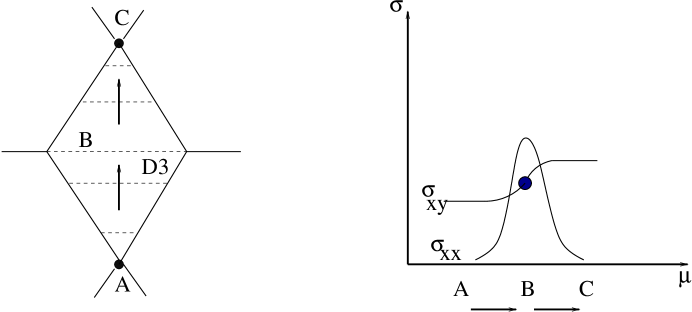
Figure 3: Brane realization of the transition between plateaux. In the position B one gets a conformal field theory

Let us explain the simplest example of such transition a little bit more precise. Suppose that 5 branes are originating in a ”diamond” configuration (see Fig.3).

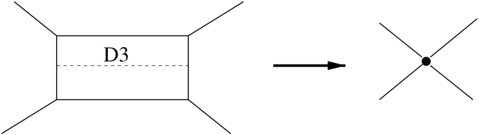
Figure 4: Box made from five-branes with a D3 brane inside.

The crucial point is that is was argued that any intersection of (p,q) 5 branes amounts to the nontrivial superconformal point in d=5 theory on 5 branes [38]. Moreover if the D3 brane is stretched between 5 branes when D3 brane moves to the these intersection points the critical d=3 theories emerge as well. Let us try to exploit this setup to explain the transitions. Our conjecture is formulated as follows. Since the quantum numbers of 5 branes fix the filling factors uniquely we start with position of D3 brane at the down vertex of the diamond. This vertex correspond to the initial fixed point of the QH RG flow at some plateau. It is clear from the conjectured brane geometry that $\sigma_{xx}=0$ at this point in agreement with the QH flows. More accurately to see the nontrivially generated CS level due to the five brane quantum numbers it is necessary to assume that the vertex itself has the internal microscopic structure (see Fig.4)

Then we move D3 brane up interpreting this motion as the RG flow. At some value of $x_{3}$ D3 brane approaches the next critical point corresponding the point of two 5 brane junctions. This critical point geometrically corresponds to $\sigma_{xx}\neq 0$ . This is consistent with the existence of the conformal fixed point at $\sigma_{xx}\neq 0$ between the plateaux. Recently it was argued that this conformal point corresponds to the noncompact SL(2,R) WZW model [39, 40]. Since the group SL(2,R) geometrically is $AdS_{3}$ we would like to ask where this $AdS_{3}$ could come from. Fortunately it can be easily found. Indeed there is nonzero density of D1 branes on D3 branes. On the other hand it is known that N D1 branes at large N creates $AdS_{3}$ geometry needed for the WZW model. This coincidence can be considered as a rough consistency check of our conjecture. Finally D3 brane reaches the upper vertex of the diamond with the other filling factor which can be calculated using the conservation of the 5 brane charges at the junction manifold.

One more evident check follows from the known logarithmic renormalization of $\sigma_{xx}$ which has to be seen in the brane picture geometrically. Namely in analogy with coupling constant renormalization in N=1 SYM theory we have to interprete this running coupling constant as the solution to the Laplace equation with a source, represented by D3 brane in $x_{4},x_{5}$ coordinates. Removing one D3 brane from the vertex we destroy the criticality and it is natural to assume that $\beta$ function comes precisely from this single D3 brane. If this interpretation is true the independence of the weak coupling $\beta$ function on the filling fractions asquires the natural explanation.

Note that the argumentation above was applied to the transitions between the integer Quantum Hall plateaux which are represented by the D3 branes with the finite extent in $x_{6}$ direction. The simplest transition between these plateuax corresponds to removing one D3 brane with some number of D1 branes from the bunch of the remaining branes. Hence, we have indeed the motion of D1 brane in the background of many D1’s providing the $AdS_{3}$ geometry. To consider the generic transitions between FQHE plateaux we have to take into account the motion the semiinfinite D3 branes along the five-brane web. It is still unclear what universality class governs the generic transitions between FQHE plateaux.

7 Discussion

In this paper we discuss several aspects of the realization of the FQHE via noncommutative Chern-Simons theory. First, we generalize the description of the FQHE system with the finite amount of electrons to the topology of the torus. We argued that the corresponding many-body system can be identified with the integrable Ruijsenaars model. Then we interpret two alternative descriptions of the model in terms of commutative and noncommutative gauge theories as the version of Morita duality.

Using the brane description of the many-body system we suggest a new IIB brane picture for the FQHE system which is based on the brane realization of CS terms via (p,q) 5 branes. It is quite transparent and can be easily generalized for the Jain and Haldane hierarchies. Moreover it implies some dualities which partially have counterparts in the FQHE system with finite or infinite number of electrons. In particular S duality as well as mirror symmetry can be identified. A brane realization of the RG flows was conjectured.

Finally one could ask even more general questions concerning the physical meaning of the extra coordinates in the context of the QHE. In SUSY gauge theories these coordinates come from the higher dimensional components of the gauge field which are interpreted as the scalar fields on the brane worldvolume. Naively there is no place for the additional scalar fields in the context of QHE so one should look for another viewpoint.

We can speculate that the additional coordinates actually could be related with the momentum space of the usual four-dimensional theory. Then the corresponding brane picture can be interpreted in terms of the Fermi surfaces similar to the interpetation of the Peierls model in [41]. The set of branes in the momentum space can be treated along this way as the result of the complicated level crossing phenomena which are known to provide the defects of the different codimensions resulting in nontrivial Berry phases. The size of the brane is related to the chemical potential. Let us note that in the “diamond” picture on Fig.3 the coordinate describing the motion in the vertical direction is related to the chemical potential. Brane motion in this direction corresponds to the transition between plateaux which in turn leads to the change in chemical potential. Note that with this interpretation we have no reference whatsoever to the Planck scale.

Let us emphasize once again that there are similarities between the brane descriptions of QHE and N=1 SUSY theories. Both theories manifest the behaviour with the dynamically generated mass gap. In $D=4$ N=1 this mass scale can be seen in the MQCD description geometrically. The same situation we expect in the M theory description of FQHE however to see this more explicitly the additional analysis is required. And most importantly both theories being the low energy ones have nothing to do with the quantum gravity scale and all degrees of quantum gravity scale are decoupled. This is absolutely important for the consisteny of the whole brane approach to the physical theories with a well-defined UV behaviour - obviously QHE as well as QCD are exactly such theories.

Finally let us briefly discuss possible brane description of CS of (quasi)planar superconducting state. It was suggested some time ago that anyon system can be in a superconducting state[42]. The transition to this state is due to emergence of massless mode - a $3D$ photon. The mass of the photon in a topologically massive gauge (Maxwell-CS) theory is proportional to CS coefficient $k$ and in superconducting state bare $k$ is completely cancelled by one-loop correction (actually it happens only at zero temperature, at nonzero $T$ there is still small mass [43]). It will be interesting to have brane realiztion for anyon superconductivity and to find what integrable model it corresponds to . In this brane picture we must have an effect of complete (at $T=0$) or partial (at $T\neq 0$) screeing of CS coupling. It will be also interesting to find brane realization of more complicated superconduction systems, like P-even anyon superconductors [44].

The work of A.G. is supported in part by grants INTAS-00-00334 and CRDF-RP1-2108, IK is supported in part by PPARC rolling grant PPA/G/O/1998/00567, both I.K. and C.K.A. are supported in part by the EC TMR grant HPRN-CT-2000-00152 and a joint CNRS-Royal Society grant.

References

- [1] M. R. Douglas and N. A. Nekrasov, “Noncommutative field theory,” hep-th/0106048.
-
[2]
A. Connes, M. R. Douglas and A. Schwarz,
“Noncommutative geometry and matrix theory: Compactification on tori,”
JHEP 9802 (1998) 003
[hep-th/9711162]
N. Seiberg and E. Witten, “String theory and noncommutative geometry,” JHEP 9909 (1999) 032 [hep-th/9908142]. - [3] A. Gonzalez-Arroyo and M. Okawa, “The Twisted Eguchi-Kawai Model: A Reduced Model For Large N Lattice Gauge Theory,” Phys. Rev. D 27 (1983) 2397.
- [4] A. Gonzalez-Arroyo and C. P. Korthals Altes, “Reduced Model For Large N Continuum Field Theories,” Phys. Lett. B 131 (1983) 396.
-
[5]
A. Schwarz,
“Morita equivalence and duality,”
Nucl. Phys. B 534, 720 (1998)
[hep-th/9805034].
C. Hofman and E. Verlinde, “Gauge bundles and Born-Infeld on the noncommutative torus,” Nucl. Phys. B 547, 157 (1999) [hep-th/9810219].
B. Pioline and A. Schwarz, “Morita equivalence and T-duality (or B versus Theta),” JHEP 9908, 021 (1999) [hep-th/9908019]. - [6] L. Susskind, “The quantum Hall fluid and non-commutative Chern Simons theory,” hep-th/0101029.
-
[7]
A. P. Polychronakos,
“Quantum Hall states as matrix Chern-Simons theory,”
JHEP 0104, 011 (2001)
[hep-th/0103013]
A. P. Polychronakos, “Quantum Hall states on the cylinder as unitary matrix Chern-Simons theory,” JHEP 0106, 070 (2001) [hep-th/0106011]. -
[8]
H. Azuma and S. Iso,
“Explicit relation of quantum hall effect and Calogero-Sutherland model,”
Phys. Lett. B 331, 107 (1994)
[hep-th/9312001].
S. Iso and S. J. Rey, “Collective field theory of the fractional quantum hall edge state and the Calogero-Sutherland model,” Phys. Lett. B 352, 111 (1995) [hep-th/9406192]. -
[9]
J. Ambjorn, Y. M. Makeenko, J. Nishimura and R. J. Szabo,
“Lattice gauge fields and discrete noncommutative Yang-Mills theory,”
JHEP 0005, 023 (2000)
[hep-th/0004147]
K. Saraikin, J.Exp. Theor. Phys. 91 (2000) 653
Z. Guralnik and J. Troost, JHEP 0105 (2001) -
[10]
J.Froehlich, A. Zee,
“Large scale physics of the quantum Hall fluid,”
Nucl. Phys. B 364 (1991) 517.
X. G. Wen and A. Zee, “Classification of Abelian quantum Hall states and matrix formulation of topological fluids,” Phys. Rev. B 46 (1992) 2290. - [11] L. Alvarez-Gaume and J. L. Barbon, “Morita duality and large-N limits,” hep-th/0109176
- [12] V. Fock, A. Gorsky, N. Nekrasov and V. Rubtsov, “Duality in integrable systems and gauge theories,” JHEP 0007, 028 (2000) [hep-th/9906235].
- [13] A. Gorsky and N. Nekrasov, “Hamiltonian systems of Calogero type and two-dimensional Yang-Mills theory,” Nucl. Phys. B 414, 213 (1994) [hep-th/9304047].
- [14] A. Gorsky and N. Nekrasov, “Relativistic Calogero-Moser model as gauged WZW theory,” Nucl. Phys. B 436 (1995) 582 [hep-th/9401017].
-
[15]
J. H. Brodie, L. Susskind and N. Toumbas,
“How Bob Laughlin tamed the giant graviton from Taub-NUT space,”
JHEP 0102, 003 (2001)
[hep-th/0010105].
B. Freivogel, L. Susskind and N. Toumbas, “A two fluid description of the quantum Hall soliton,” hep-th/0108076.
S. S. Gubser and M. Rangamani, “D-brane dynamics and the quantum Hall effect,” JHEP 0105, 041 (2001) [hep-th/0012155]. -
[16]
O. Bergman, Y. Okawa and J. H. Brodie,
“The stringy quantum Hall fluid,”
hep-th/0107178
S. Hellerman and L. Susskind, “Realizing the quantum Hall system in string theory,” hep-th/0107200. - [17] A. Gorsky and A. Mironov, “Integrable many-body systems and gauge theories,” hep-th/0011197.
-
[18]
T. Kitao, K. Ohta and N. Ohta,
“Three-dimensional gauge dynamics from brane configurations with (p,q)-fivebrane,”
Nucl. Phys. B 539, 79 (1999)
[hep-th/9808111]
O. Bergman, A. Hanany, A. Karch and B. Kol, “Branes and supersymmetry breaking in 3D gauge theories,” JHEP 9910, 036 (1999) [hep-th/9908075]. - [19] A. El Rhalami, E. M. Sahraoui and E. H. Saidi, “NC branes and hierarchies in quantum Hall fluids,” hep-th/0108096.
-
[20]
M. A. Olshanetsky and A. M. Perelomov,
“Classical Integrable Finite Dimensional Systems Related To Lie Algebras,”
Phys. Rept. 71 (1981) 313.
M. A. Olshanetsky and A. M. Perelomov, “Quantum Integrable Systems Related To Lie Algebras,” Phys. Rept. 94 (1983) 313. - [21] N. Nekrasov, “On a Duality in Calogero-Moser-Sutherland Systems,” hep-th/970711
- [22] A. P. Polychronakos, “Integrable systems from gauged matrix models,” Phys. Lett. B 266 (1991) 29.
-
[23]
S. Hellerman and M. Van Raamsdonk,
“Quantum Hall physics equals noncommutative field theory,”
hep-th/0103179.
D. Karabali and B. Sakita, “Chern-Simons matrix model: Coherent states and relation to Laughlin wavefunctions,” hep-th/0106016. - [24] S. Kivelson, D-H. Lee and S-C. Zhang, Phys. Rev. B 46, 2223, (1992)
- [25] C.A. Lutken and G.G. Ross, Phys. Rev. B 48, 2500, (1993)
- [26] C. P. Burgess, R. Dib and B. P. Dolan, “Derivation of the Semi-circle Law from the Law of Corresponding States,” arXiv:cond-mat/9911476.
- [27] B. P. Dolan, “Duality and the Modular Group in the Quantum Hall Effect,” J. Phys. A 32 (1999) L243 [cond-mat/9805171].
-
[28]
H. Levine, S. B. Libby and A. M. Pruisken,
“Electron Delocalization By A Magnetic Field In Two-Dimensions,”
Phys. Rev. Lett. 51 (1983) 1915
D.E. Khmel’nitskii, JETP Lett. 38, 552, (1983)
A.M. Pruisken, Phys. Rev. Lett. 61, 1297 (1988) - [29] C. P. Burgess and B. P. Dolan, “Particle-vortex duality and the modular group: Applications to the quantum Hall effect and other 2-D systems,” hep-th/0010246
- [30] C. P. Burgess and C. A. Lutken, “One-dimensional flows in the quantum Hall system,” Nucl. Phys. B 500 (1997) 367 [cond-mat/9611118].
- [31] N. Seiberg, “Electric - magnetic duality in supersymmetric nonAbelian gauge theories,” Nucl. Phys. B 435, 129 (1995) [hep-th/9411149].
- [32] V. A. Novikov, M. A. Shifman, A. I. Vainshtein and V. I. Zakharov, “Exact Gell-Mann-Low Function Of Supersymmetric Yang-Mills Theories From Instanton Calculus,” Nucl. Phys. B 229, 381 (1983).
-
[33]
M. Gaudin, SPhT-92-158
S. Iso, “Anyon basis of c = 1 conformal field theory,” Nucl. Phys. B 443 (1995) 581 [hep-th/9411051]
J. A. Minahan and A. P. Polychronakos, Phys. Rev. B 50 (1994) 4236 [arXiv:hep-th/9404192
Z. N. Ha, “Exact dynamical correlation functions of Calogero-Sutherland model and one-dimensional fractional statistics,” Phys. Rev. Lett. 73 (1994) 1574 - [34] A. Kapustin and M. J. Strassler, “On mirror symmetry in three dimensional Abelian gauge theories,” JHEP 9904 (1999) 021 [hep-th/9902033].
-
[35]
E. Witten,
“Supersymmetric index of three-dimensional gauge theory,”
hep-th/9903005
K. Ohta, “Supersymmetric index and s-rule for type IIB branes,” JHEP 9910, 006 (1999) [hep-th/9908120 - [36] L. Cooper, I. I. Kogan, A. Lopez and R. J. Szabo, “Dual response models for the fractional quantum Hall effect,” Phys. Rev. B 58, 7893 (1998) [cond-mat/9712233]
-
[37]
L. Cooper, I. I. Kogan and R. J. Szabo,
“Mirror maps in Chern-Simons gauge theory,”
Annals Phys. 268, 61 (1998)
[hep-th/9710179].
I. I. Kogan, A. Momen and R. J. Szabo, “Induced dilaton in topologically massive quantum field theory,” JHEP 9812, 013 (1998) [hep-th/9811006]. -
[38]
O. Aharony and A. Hanany,
“Branes, superpotentials and superconformal fixed points,”
Nucl. Phys. B 504 (1997) 239
[hep-th/9704170].
O. Aharony, A. Hanany and B. Kol, “Webs of (p,q) 5-branes, five dimensional field theories and grid diagrams,” JHEP 9801 (1998) 002 [hep-th/9710116]. - [39] M. R. Zirnbauer, “Conformal field theory of the integer quantum Hall plateau transition,” hep-th/9905054.
-
[40]
M. J. Bhaseen, I. I. Kogan, O. A. Solovev, N. Taniguchi and A. M. Tsvelik,
“Towards a Field Theory of the Plateau Transitions in the Integer Quantum Hall Effect,”
Nucl. Phys. B 580 (2000) 688
[cond-mat/9912060]—
I. I. Kogan and A. M. Tsvelik, “Logarithmic operators in the theory of plateau transition,” Mod. Phys. Lett. A 15, 931 (2000) [hep-th/9912143]. - [41] A. Gorsky, “Peierls model and vacuum structure in the N = 2 supersymmetric field theories,” Mod. Phys. Lett. A 12, 719 (1997) [hep-th/9605135].
-
[42]
V. Kalmeyer and R. B. Laughlin,
“Equivalence Of The Resonating Valence
Bond And Fractional Quantum Hall States,”
Phys. Rev. Lett. 59 (1987) 2095
R. B. Laughlin, “Supercondcuting Ground State Of Noninteracting Particles Obeying Fractional Statistics,” Phys. Rev. Lett. 60 (1988) 2677
A. L. Fetter, C. B. Hanna and R. B. Laughlin, “Random Phase Approximation In The Fractional Statistics Gas,” Phys. Rev. B 39 (1989) 9679.
Y. H. Chen, F. Wilczek, E. Witten and B. I. Halperin, “On Anyon Superconductivity,” Int. J. Mod. Phys. B 3 (1989) 1001.
M. Greiter, F. Wilczek and E. Witten, “Hydrodynamic Relations In Superconductivity,” Mod. Phys. Lett. B 3 (1989) 903. - [43] J. D. Lykken, J. Sonnenschein and N. Weiss, “Anyonic Superconductivity,” Phys. Rev. D 42 (1990) 2161.
-
[44]
A. Kovner and B. Rosenstein,
Phys. Rev. B42, 4748 (1990)
N. Dorey and N. E. Mavromatos, Phys. Lett. B 250 (1990) 107
G. W. Semenoff and N. Weiss, Phys. Lett. B 250, 117 (1990). - [45] M. Asorey, F. Falceto and G. Sierra, “Chern-Simons theory and BCS superconductivity,”hep-th/0110266.
- [46] A. Gorsky, N. Nekrasov and V. Rubtsov, “Hilbert schemes, separated variables, and D-branes,” Commun. Math. Phys. 222 (2001) 299 [hep-th/9901089].