LBNL-49078

UCB-PTH-01/40

UFIFT-HEP-01-20

hep-th/0110301

A Worldsheet Description of Large $N_{c}$ Quantum Field Theory

Korkut Bardakci and Charles B. Thorn

Department of Physics, University of California, Berkeley CA 94710 and Theoretical Physics Group, Lawrence Berkeley National Laboratory
University of California, Berkeley CA 94710

The $N_{c}\rightarrow\infty$ limit of a matrix quantum field theory is equivalent to summing only planar Feynman diagrams. The possibility of interpreting this sum as some kind world-sheet theory has been in the air ever since ’t Hooft’s original paper. We establish here just such a world sheet description for a scalar quantum field with interaction term $g{\rm Tr}\phi^{3}/\sqrt{N_{c}}$, and we indicate how the approach might be extended to more general field theories.

1 Introduction

Almost from the beginning of the development of string theory there has been the suspicion that underlying it is a local quantum field theory. The first concrete proposal of such a connection was the fishnet diagram model of Nielsen and Olesen and Sakita and Virasoro [1]. These authors suggested identifying the string worldsheet with very large planar diagrams.

Then ’t Hooft showed how to single out the planar diagrams of an $N_{c}\times N_{c}$ matrix quantum field theory by taking the limit $N_{c}\rightarrow\infty$ [2]. However, the large fishnet diagrams are only a tiny subset of the surviving planar diagrams in this limit, and so it was not at all clear how to interpret the sum of them all as a string worldsheet. Thus there was the suggestion that strong ’t Hooft coupling $\lambda=N_{c}g^{2}$ was really needed to force the dominance of the large fishnet diagrams with a consequent worldsheet interpretation of that double limit [3, 4]. Another version of this idea was given in [5, 6, 7] where large planar diagrams were enhanced by going to a critical ’t Hooft coupling as well as large $N_{c}$. The need for this double limit has also arisen in the more modern version of the string/QFT connection as proposed by Maldacena [8, 9, 10]. Other recent work on worldsheets from large planar diagrams can be found in [11, 12].

But, in addition to his association of planar diagrams with the $N_{c}\rightarrow\infty$ limit, ’t Hooft also hinted at a way to associate a smooth world sheet with each planar diagram, large or small, at least in light-cone gauge [2]. If such a formulation is possible, the sum of the planar diagrams of a quantum field theory can be thought of in the same way as the sum of interacting open string diagrams [13, 14]. We think such a formulation of the sum of all planar diagrams would be an important step toward understanding the string/QFT connection. For example, if properly formulated one might be able to identify a worldsheet order parameter whose expectation would be the string tension. One might then hope to learn a lot about the physics of the emergent string by following the consequences of such a non-vanishing order parameter, even if a complete solution of the dynamics is not available.

In this article we give such an interpretation for the particularly simple case of the planar diagrams of a massless scalar field theory with cubic interactions. We are not concerned here about the intrinsic instability of this theory, because our construction is a reinterpretation of each individual Feynman diagram in terms of a world sheet, i.e. it works order by order in perturbation theory. Thus our real aim is to provide a paradigm for a worldsheet description of the planar diagrams of a wide range of quantum field theories.

We shall use light-cone quantization in our initial construction, although we shall see that the resulting light-cone worldsheet model can be extended to a covariant description. In the context of the light-cone description, one can understand the physics underlying our approach by considering the infinite rest tension limit of string theory, which is supposed to be a quantum field theory. The planar multi-loop diagrams of the string theory should then go over to the planar multi-loop diagrams of the limiting field theory. But the light-cone string treats $p^{+}$ in a very special way. The parameter $\sigma$ marking points on the string is chosen so that the $p^{+}$ density is unity so $p^{+}$ is just the length of the parameter interval $0\leq\sigma\leq p^{+}$. To think more clearly about what this means, it is helpful to discretize $\sigma=lm$, $l=1,\ldots,M$ and hence $p^{+}=Mm$. Then the string is a bound composite system of string bits, each carrying one unit $p^{+}$. If one takes the $T_{0}\rightarrow\infty$ limit of the light-cone multi-loop diagrams discretized in this way, the string is indeed tightly bound in transverse space, but the $p^{+}$ it carries is still uniformly distributed among the bits [15]. From this it is clear what we need to do. We must think of a field quantum carrying $p^{+}=Mm$, not as a single particle with $M$ units of $p^{+}$, but rather as $M$ bits, each with one unit of $p^{+}$.

But this entails introducing transverse coordinates and momenta for each bit. Our construction places these bit degrees of freedom in the bulk of the worldsheet. All but one of these degrees of freedom must be redundant, so we expect that the worldsheet we construct will be “topological” in the sense that all the physics must live on the boundaries. Thus our work has parallels with other studies of topological string theories, see for example [16].

In Section 2 we begin our work by constructing a local world sheet representation of the free scalar propagator on the light-cone. In Section 3 we show how the light-cone worldsheet action we infer can be extended to a covariant one. In Section 4 we extend the construction to include the cubic interactions of ${\rm Tr}\phi^{3}$ matrix field theory and propose a worldsheet path integral which sums all of the planar loop diagrams by coupling the worldsheet variables to an Ising spin system set up on the sites of the world sheet. In Section 5 we give a representation of this Ising spin system in terms of Grassmann integration. This new formulation allows the continuum limit of the coupled Ising system to be taken at least formally. In Section 6 we delve into the issue of giving the fields a mass. In a short section 7 we indulge in some amusing comments on duality between string worldsheets and QFT worldsheets. Finally, in Section 8 we give a list of the many generalizations and potential developments we leave for the future.

2 Free Massless Scalar Field

In this section we shall use light-cone coordinates defined as $x^{\pm}=(x^{0}\pm x^{3})/\sqrt{2}$. The remaining components of $x^{\mu}$ will be distinguished by Latin indices, or as a vector by bold-face type. Thus the four coordinates $x^{\mu}$ will be $(x^{+},x^{-},{\bf x})$ or $(x^{+},x^{-},x^{k})$. We shall similarly use the same conventions for the components of any four vector. Thus the Lorentz invariant scalar product of two four vectors $v,w$ is written $v\cdot w={\bf v}\cdot{\bf w}-v^{+}w^{-}-v^{-}w^{+}$. We shall select $x^{+}$ to be our quantum evolution parameter, and recall that the “energy” conjugate to this time is $p^{-}$. A massless on-shell particle thus has the “energy” $p^{-}={\bf p}^{2}/2p^{+}$.

We begin our discussion with the mixed representation of the propagator of free massless matrix scalar field [2]:

$$\langle\phi_{\alpha}^{\beta}(x^{+})\phi_{\gamma}^{\delta}(0)\rangle\equiv\delta_{\alpha}^{\delta}\delta_{\gamma}^{\beta}\int{dp^{-}\over 2\pi i}e^{-ix^{+}p^{-}}{1\over p^{2}-i\epsilon}=\delta_{\alpha}^{\delta}\delta_{\gamma}^{\beta}{\theta(x^{+})\over 2p^{+}}e^{-ix^{+}{\bf p}^{2}/2p^{+}}\rightarrow\delta_{\alpha}^{\delta}\delta_{\gamma}^{\beta}{\theta(\tau)\over 2p^{+}}e^{-\tau{\bf p}^{2}/2p^{+}},$$ (1)

where we assume $p^{+}>0$. Since we shall consider only planar diagrams in this paper, we shall suppress the color factors $\delta_{\alpha}^{\delta}\delta_{\gamma}^{\beta}$ in the rest of the paper. Note that we have defined imaginary time $\tau=ix^{+}$. We use imaginary $x^{+}$ for convenience to make our integrals damped instead of rapidly oscillating. It is certainly not essential for our purposes. For instance, we shall return to real time when discussing the classical limit. The expression (1) is the starting point for our worldsheet construction.

Based on the analogy of the light-cone string [17], ’t Hooft associated this propagator with a rectangular world sheet of width $p^{+}$ and length $\tau$. The suppressed color factors are associated with spatial boundaries of this rectangle. We shall do the same. The expression for the propagator, however, is not yet associated in any way with local variables on this world sheet.

To facilitate the introduction of such local variables we set up a lattice worldsheet by discretizing $\tau$ and $p^{+}$:

$$\tau=ka,\qquad p^{+}=lm,\qquad{\rm for}\quad k,l=1,2,3,\ldots$$ (2)

Then the scalar propagator becomes

$${\theta(k)\over 2lm}e^{-k(a/m){\bf p}^{2}/2l}$$ (3)

The factor $1/2lm$ is better associated with one of the two vertices to which the line is attached. Here we have a choice between assigning the factors symmetrically by using square roots, or asymmetrically. The asymmetry is natural in light-cone parameterization because all propagation is forward in time. Thus we can, for example, assign the factor to the earlier of the two vertices connected by the line. Then a fission vertex, in which one particle with $p^{+}=Mm$ “decays” to two particles with $p^{+}_{1}=M_{1}m$, $p^{+}_{2}=M_{2}m$ will be assigned the factor $1/4M_{1}M_{2}m^{2}$, whereas a fusion vertex, which is the time-reversal of the fission vertex will be assigned the factor $1/2Mm$. After assigning the prefactors in this way, all propagators are then simple exponentials $e^{-ka{\bf p}^{2}/2lm}$.

Consider a line carrying $M$ units of $p^{+}$. As in [2] it will be convenient to write the total momentum as a difference ${\bf p}\equiv{\bf q}_{M}-{\bf q}_{0}$. For each discrete time step, we notice that one can write

$$\exp\left\{-{a\over m}{({\bf q}_{M}-{\bf q}_{0})^{2}\over 2M}\right\}=M^{d/2}\left({a\over 2\pi m}\right)^{d(M-1)/2}\int d{\bf q}_{1}d{\bf q}_{2}\cdots d{\bf q}_{M-1}e^{-{a}\sum_{i=0}^{M-1}({\bf q}_{i+1}-{\bf q}_{i})^{2}/2m}.$$ (4)

We would like to use this identity to interpret a line carrying $M$ units of $p^{+}$ as $M$ lines, each carrying a single unit of $p^{+}$. At first sight it seems that the factors multiplying the integral obstruct this interpretation. Indeed, there is an essential difference between a single particle state and a multi-particle state, in that the latter has many momenta assigned to it, i.e. the phase space is much larger. The extra particles must be “fictitious” in some appropriate sense. Alternatively, there must be some strong binding force that binds the many particles together to act as a single particle [15]. In this article we choose the former possibility.

To achieve this “fictitiousness”, we introduce a pair of anti-commuting ghost fields $b_{i},c_{i}$ for every two transverse dimensions. Consider then the ghost integrals

$$\int\prod_{i=1}^{M-1}dc_{i}db_{i}\exp\left\{\sum_{i=0}^{M-1}(b_{i+1}-b_{i})(c_{i+1}-c_{i})\right\} = Me^{(b_{M}-b_{0})(c_{M}-c_{0})/M}$$ (5)

$$= M\qquad{\rm for}\quad c_{0}=c_{M}=0,b_{0}=b_{M}=0.$$

To get the required factor of $M$ we adopt the Dirichlet conditions indicated. For simplicity of presentation, let us restrict our attention to the case $d=2$, which is actually the case of most interest (four dimensional space-time). For this case we only require one $b,c$ set of ghosts. Then, we may rewrite the identity of Eq (4)

$$\exp\left\{-{a\over m}{({\bf q}_{M}-{\bf q}_{0})^{2}\over 2M}\right\} =$$ (6)

$$\hskip-85.35826pt\int\prod_{i=1}^{M-1}{dc_{i}db_{i}\over 2\pi}d{\bf q}_{i}\exp\left\{{a\over m}\sum_{j=0}^{M-1}(b_{j+1}-b_{j})(c_{j+1}-c_{j})-{a\over 2m}\sum_{i=0}^{M-1}({\bf q}_{i+1}-{\bf q}_{i})^{2}\right\},$$

where we recall that we have imposed $c_{0}=b_{0}=c_{M}=b_{M}=0$. To build the propagator for $N$ time steps, we merely repeat this construction $N$ times:

$$\exp\left\{-N{a\over m}{({\bf q}_{M}-{\bf q}_{0})^{2}\over 2M}\right\} =$$ (7)

$$\hskip-142.26378pt\int\prod_{j=1}^{N}\prod_{i=1}^{M-1}{dc^{j}_{i}db^{j}_{i}\over 2\pi}d{\bf q}^{j}_{i}\exp\left\{{a\over m}\sum_{j}\sum_{i=0}^{M-1}(b^{j}_{i+1}-b^{j}_{i})(c^{j}_{i+1}-c^{j}_{i})-{a\over 2m}\sum_{j}\sum_{i=0}^{M-1}({\bf q}^{j}_{i+1}-{\bf q}^{j}_{i})^{2}\right\}.$$

The expression (7) implements momentum conservation essentially “by hand”. The momentum propagated ${\bf p}={\bf q}_{M}-{\bf q}_{0}$ is conserved by the imposition of the Dirichlet boundary conditions ${\bf q}_{0,j}={\bf q}_{0}$ and ${\bf q}_{M,j}={\bf q}_{M}$. To incorporate these conditions in the world sheet path integral requires the insertion of delta functions that conserve these boundary values from one time slice to the next. This will be a crucial refinement for the description of multi-loop diagrams. The most economical approach is to retain the Dirichlet boundary condition at one end of the strip, say $i=0$, where we impose ${\bf q}_{0}^{j}={\bf q}_{0}$ but insert momentum conserving delta functions at the other end $i=M$. It is convenient but not necessary to set ${\bf q}_{0}=0$. In fact the particle transition amplitude should have these delta functions explicitly incorporated:

$$T_{fi}=\langle{\bf p}_{f}|e^{-\tau p^{-}}|{\bf p}\rangle = \delta({\bf p}_{f}-{\bf p})e^{-\tau{\bf p}^{2}/2p^{+}}$$

$$\rightarrow \int\prod_{j=1}^{N}d{\bf q}_{M}^{j}\prod_{j=0}^{N}\delta({\bf q}_{M}^{j+1}-{\bf q}_{M}^{j})e^{-a\sum_{j}({\bf q}_{M}^{j}-{\bf q}_{0})^{2}/2p^{+}}$$

$$= \int\prod_{j=1}^{N}d{\bf q}_{M}^{j}\prod_{j=0}^{N}{d{\bf x}_{M}^{j}\over(2\pi)^{d}}e^{-i{\bf x}_{M}^{j}\cdot({\bf q}_{M}^{j+1}-{\bf q}_{M}^{j})}e^{-a\sum_{j}({\bf q}_{M}^{j}-{\bf q}_{0})^{2}/2mM}.$$ (9)

The complete path integral is then reached by inserting (7) for $d=2$.

$$T_{fi} = \int\prod_{j=1}^{N}\prod_{i=1}^{M}{dc^{j}_{i}db^{j}_{i}\over 2\pi}d{\bf q}^{j}_{i}\prod_{j=0}^{N}{d{\bf x}_{M}^{j}\over(2\pi)^{2}}\exp\left\{-i\sum_{j=0}^{N}{\bf x}_{M}^{j}\cdot({\bf q}_{M}^{j+1}-{\bf q}_{M}^{j})\right\}$$ (10)

$$\hskip 0.0pt\exp\left\{{a\over m}\sum_{j}\sum_{i=0}^{M-1}(b^{j}_{i+1}-b^{j}_{i})(c^{j}_{i+1}-c^{j}_{i})-{a\over 2m}\sum_{j}\sum_{i=0}^{M-1}({\bf q}^{j}_{i+1}-{\bf q}^{j}_{i})^{2}\right\}.$$

This completes the worldsheet construction for the propagator for a free scalar field. It is represented by a strip of length $T=(N+1)a$ and width $p^{+}=Mm$. The discretized world-sheet is a rectangular grid. Each site carries a momentum variable ${\bf q}_{i}^{j}$ and a pair of ghost fields $b_{i}^{j},c_{i}^{j}$. In addition the sites at the $i=M$ boundary carry coordinates ${\bf x}_{M}^{j}$. The discretized world sheet action is just the exponent appearing in (10). The total transverse momentum carried by the propagator is the difference of the momenta, ${\bf p}={\bf q}_{M}-{\bf q}_{0}$, at the boundaries of the strip, which are fixed by the Dirichlet conditions imposed by the delta functions. Notice that there are no terms in the bulk action coupling different time slices: the free world sheet dynamics is “constrained” or topological. For the free propagator time slice couplings occur only at the boundaries. When we draw discretized worldsheet diagrams (see Fig. 2), with time flowing up, we shall distinguish the bulk and boundary degrees of freedom by dotted and solid vertical lines respectively. As we shall see, the field theoretic interactions will gradually introduce more time slice couplings, via the insertion of new Dirichlet boundaries (indicated by solid lines) within the worldsheet, order by order in perturbation theory.

In the next section we discuss the continuum path integral in a more general parameterization than light-cone, so that we can expose the Lorentz covariance of the description more clearly. For this purpose it is convenient to write the boundary terms involving the coordinates as a topological bulk expression. We remark here that we can do this even at the discretized level by noting the equality

$$\sum_{j=0}^{N}{\bf x}_{M}^{j}\cdot({\bf q}_{M}^{j+1}-{\bf q}_{M}^{j}) = \sum_{j=1}^{N}\sum_{i=0}^{M-1}\left[({\bf x}_{i+1}^{j}-{\bf x}_{i}^{j})\cdot({\bf q}_{i}^{j+1}-{\bf q}_{i}^{j})-({\bf x}_{i+1}^{j}-{\bf x}_{i+1}^{j-1})\cdot({\bf q}_{i+1}^{j}-{\bf q}_{i}^{j})\right]$$ (11)

$$\hskip 56.9055pt+S_{N}-S^{\prime}_{0},$$

where the last two terms only involve variables at final and initial times $j=N,N+1$ and $j=0,1$ respectively. They therefore do not affect the dynamics described by the free field propagator.

3 Continuum Limit and Lorentz Invariance

3.1 Free Propagator

In this section we give a first discussion of the continuum limit of the world sheet construction for the free propagator. We note that the worldsheet path integral has the formal continuum limit

$$T_{fi} = \int DcDbD{\bf q}D{\bf x}\exp\left\{i\int d\tau d\sigma\left({\bf\dot{x}}\cdot{\bf q}^{\prime}-{\bf x}^{\prime}\cdot{\bf\dot{q}}\right)\right\}\prod_{\sigma,\tau}\delta({\bf x}^{\prime}(\sigma,\tau))$$ (12)

$$\exp\left\{\int_{0}^{T}d\tau\int_{0}^{p^{+}}d\sigma b^{\prime}(\sigma,\tau)c^{\prime}(\sigma,\tau)-{1\over 2}\int_{0}^{T}d\tau\int_{0}^{p^{+}}d\sigma{\bf q}^{\prime}(\sigma,\tau)^{2}\right\}.$$

To interpret this formula more covariantly, we first of all return to real time, $\tau\rightarrow i\tau$, and extend the transverse components of momentum $q^{k}(\sigma,\tau)$ to a four vector $q^{\mu}(\sigma,\tau)$ by introducing $q^{\pm}(\sigma,\tau)$. Then we recognize that we have actually fixed the $\sigma$ parameter so that $q^{+}(\sigma,\tau)=\sigma$ or $q^{+\prime}(\sigma,\tau)=1$. Then we have

$$q^{\prime}\cdot q^{\prime}={\bf q^{\prime}}^{2}-2q^{+\prime}q^{-\prime}={\bf q^{\prime}}^{2}-2q^{-\prime}.$$

The last term in the second exponent of (12) just represents the energy contribution to the action $-\int d\tau p^{-}$. With our identification of momentum components as differences, $p^{-}=q_{1}^{-}-q^{-}_{0}=\int d\sigma q^{-\prime}$, we see that this identification follows in this parameterization from the covariant constraint $q^{\prime}\cdot q^{\prime}=0$. This suggests that we start in a more general parametrization with the action

$$S=\int d\tau\int_{\sigma_{0}(\tau)}^{\sigma_{1}(\tau)}d\sigma\left({\dot{x}}\cdot{q^{\prime}}-{x^{\prime}}\cdot{\dot{q}}-{\lambda\over 2}q^{\prime 2}\right)$$ (13)

where $\lambda$ is a Lagrange multiplier enforcing the constraint $q^{\prime 2}=0$, and we recall that the value of $q^{\mu}$ is fixed at $\sigma=\sigma_{0}(\tau)$.

We notice the invariances of (13). There is invariance under a partial reparametrization under

$$\sigma\rightarrow\sigma(\tau^{\prime},\sigma^{\prime}),\qquad\tau\rightarrow\tau(\tau^{\prime}).$$ (14)

In addition, due to the topological nature of the first term in the action, there is a bulk gauge invariance

$$x^{\mu}(\sigma,\tau)\rightarrow x^{\mu}(\sigma,\tau)+\Lambda^{\mu}(\sigma,\tau),\qquad{\rm with}\quad\Lambda(\sigma_{1},\tau)=0.$$ (15)

The restriction to $\Lambda(\sigma_{1})=0$ is necessary because of the boundary value of ${\bf x}$ appears explicitly in the action.

We would like to point out that it is possible to start with an action invariant under an even larger group, namely, unrestricted reparametrizations:

$$\sigma\rightarrow\sigma(\tau^{\prime},\sigma^{\prime}),\;\;\tau\rightarrow\tau(\tau^{\prime},\sigma^{\prime}).$$ (16)

This is achieved by introducing the usual world sheet metric $g^{\alpha\beta}$ and writing

$$S=\int d\tau\int d\sigma({\dot{x}}\cdot q^{\prime}-x^{\prime}\cdot{\dot{q}}+g^{\alpha\beta}\partial_{\alpha}q\cdot\partial_{\beta}q),$$ (17)

where $\alpha=0$ refers to $\tau$ and $\alpha=1$ to $\sigma$. In addition, we impose the crucial constraint

$$\det(g)=0.$$ (18)

This constraint distinguishes our action from the usual string action. There is no conformal gauge available anymore; instead, one can gauge fix partially by setting all the components of $g^{\alpha\beta}$, with the exception of $g^{11}$ equal to zero. Identifying $g^{11}$ with $-\lambda/2$, the form of the action given by Eq (13) is then recovered, with its residual reparametrization invariance. We will not pursue this more general formulation further in this paper, however, it may provide a better starting point for possible future investigations.

As a check of our proposed action, we now show how to regain the completely gauge fixed action from (13) by exploiting the local symmetries (14,15). First, we fix $\sigma$ reparametrization invariance by choosing $\sigma=q^{+}$. Then the $x^{-\prime}$ term drops out of the action and the equation of motion for $x^{-}$ is simply $p^{+}$ conservation. As in the light-cone string this condition is conveniently implemented by restricting the $\sigma$ parameter range to $\tau$ independent boundaries: $\sigma_{0}=q^{+}_{0}$, $\sigma_{1}=q^{+}_{1}$. After these choices the action reduces to

$$S=\int d\tau\int_{q^{+}_{0}}^{q^{+}_{1}}d\sigma\left({\bf\dot{x}}\cdot{{\bf q}^{\prime}}-{\dot{x}}^{+}q^{-\prime}-{\bf x}^{\prime}\cdot{{\bf\dot{q}}}+x^{+\prime}{\dot{q}}^{-}-{\lambda\over 2}\left({\bf q}^{\prime 2}-2q^{-\prime}\right)\right)$$ (19)

Integrating out $q^{-}$ then gives $\lambda^{\prime}=0$ and $\lambda(\sigma_{1})={\dot{x}}^{+}(\sigma_{1})$, leading to

$$S=\int d\tau\int_{q^{+}_{0}}^{q^{+}_{1}}d\sigma\left({\bf\dot{x}}\cdot{{\bf q}^{\prime}}-{\bf x}^{\prime}\cdot{{\bf\dot{q}}}-{{\dot{x}}^{+}(\sigma_{1},\tau)\over 2}\ {\bf q}^{\prime 2}\right)$$ (20)

The gauge invariance (15) can now be exploited to set ${\bf x}^{\prime}=0$, as a constraint in the path integral. At the same time we are also free to set $x^{+\prime}=0$, since only $x^{+}(\sigma_{1},\tau)$ remains in the action. With $x^{+}$ independent of $\sigma$, we use the $\sigma$ independent $\tau$ reparametrization invariance to choose $x^{+}=\tau$, giving finally

$$S=\int d\tau\left[{\bf\dot{x}}\cdot({\bf q}_{1}(\tau)-{\bf q}_{0})-{1\over 2}\int_{0}^{p^{+}}d\sigma\ {\bf q}^{\prime 2}\right]\rightarrow\int d\tau\left[-{\bf x}\cdot{\bf\dot{q}}_{1}(\tau)-{1\over 2}\int_{0}^{p^{+}}d\sigma\ {\bf q}^{\prime 2}\right]$$ (21)

as desired.

Finally, we discuss Fadeev-Popov ghosts. Since we are able to completely eliminate the $\pm$ components of $x,q$ by our parametrization choice, we have also implicitly eliminated the corresponding ghosts. However, the bulk transverse components remain, and we should retain those gauge fixing ghosts. Since the gauge condition on ${\bf x}$ was ${\bf x}^{\prime}=0$, the corresponding F-P determinant is

$$({\det}_{\rm ND}(i\partial/\partial\sigma))^{d}=({\det}_{\rm ND}(-\partial^{2}/\partial\sigma^{2}))^{d/2}=1.$$

Here the subscript $\rm ND$ indicates mixed Neumann-Dirichlet boundary conditions due to the restrictions (see (15) on the gauge parameter for $x$. To see that this determinant is unity, put $c_{0}=b_{0}=0$ and integrate over $c_{M},b_{M}$ in the first of Eqs. (5).

In contrast, the Parisi-Sourlas ghost factor in (12) is ${\det}_{DD}(-\partial^{2}/\partial\sigma^{2})$ with Dirichlet conditions at both ends. We can identify this factor as a Fadeev-Popov determinant if we interpret the ${\bf q}^{\prime 2}$ term in (12) as a Feynman-style gauge fixing term for the ${\bf q}$ gauge invariance

$${\bf q}(\sigma,\tau)\rightarrow{\bf q}(\sigma,\tau)+{\bf\Lambda}^{\prime}(\sigma,\tau),\qquad{\rm with}\quad{\bf\Lambda}^{\prime}(\sigma_{0},\tau)={\bf\Lambda}^{\prime}(\sigma_{1},\tau)=0,$$ (22)

enjoyed by the topological part of $S$. Here the restriction on ${\bf\Lambda}^{\prime}$ is necessary because ${\bf q}$ satisfies Dirichlet conditions at both ends. The F-P factor for this gauge fixing is the determinant of the same differential operator as in the $x$ case, but this time with Dirichlet conditions at both ends, i.e. precisely the ghost factor shown in (12).

3.2 Interactions

The above discussion dealt exclusively with the free propagator. When interactions are included as in the following section, we must generalize the discussion of covariance to the more general case of a worldsheet with internal solid lines as well as external boundaries. Our starting point is Eq.(13), but with the boundaries unspecified at the moment. When applied to a free propagator, the variables $x$ and $q$ were continuous, except possibly at the boundaries. The generalization to the interacting case is accomplished by allowing $x$ to be discontinuous along various segments of curves (see Fig. 1).

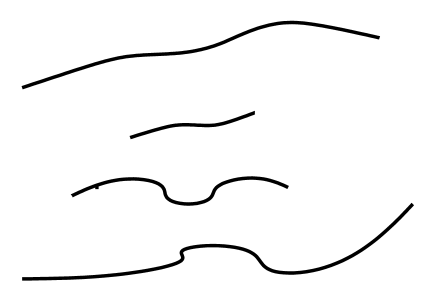
Figure 1: World sheet in a general parameterization: none of the solid lines need be straight.

In contrast, $q$ is restricted to be continuous everywhere. The beginning and the end of the segment is where the interaction takes place, and the functional integral involves a sum over all possible segments and all possible discontinuities. This sum is not well defined till we fix the parameters $\sigma$ and $\tau$, which we will do next. Making use of the $\sigma$ reparametrization invariance (14), we choose $\sigma=q^{+}$, as above. Since $q^{+}$, which is the same as $p^{+}$ with a suitable boundary condition, is conserved, the segments of discontinuity become straight lines, located at various constant values of $\sigma$. Let the nth segment be at $\sigma=\sigma_{n}$, with the end points beginning at $\tau=\tau_{n}^{i}$ and ending at $\tau_{n}^{f}$. The functional integral over the segments then reduces to ordinary integrals over $\sigma_{n}$, $\tau_{n}^{i}$, and $\tau_{n}^{f}$, plus a sum over the number of segments. These then correspond to the solid lines of Fig.(2).

Next we use the gauge invariance (15) to eliminate the variable $x$. It is important to realize that, in contrast to $x$, the gauge parameter $\Lambda$ is continuous everywhere. Therefore, we can gauge away all of $x$, except for its discontinuity across a solid line. Or alternatively, since the term

$$\dot{x}\cdot q^{\prime}-x^{\prime}\cdot\dot{q}=\frac{1}{2}\partial_{\tau}(x\cdot q^{\prime}-q\cdot x^{\prime})-\frac{1}{2}\partial_{\sigma}(x\cdot\dot{q}-q\cdot\dot{x})$$

is an exact differential, it can be integrated out, leaving behind boundary contributions from the solid lines, where x is discontinuous. As a result, S can be rewritten as

$$S=-\frac{1}{2}\int d\tau\int d\sigma\,\lambda\,q^{\prime 2}+\sum_{n}\int d\tau\,y(\sigma_{n},\tau)\cdot\dot{q}(\sigma_{n},\tau),$$ (23)

where $y$ denotes the discontinuity of $x$ across a solid line.

We now investigate the equations of motion resulting from this action , with the gauge choice $\sigma=q^{+}$. The equation obtained by varying $q^{-}$ gives

$$\frac{1}{2}\lambda^{\prime}=\sum_{n}\dot{y}^{+}_{n}\delta(\sigma-\sigma_{n}),$$ (24)

with $y^{+}_{n}=y^{+}(\sigma_{n},\tau)$. This means that $\lambda$ is a constant, except for jumps across the solid lines. We can eliminate these discontinuities with a suitable $\tau$ reparametrization, since we are allowed independent $\tau$ reparametrization in each strip bounded by solid lines. By choosing two different $\tau$ reparametrizations $\tau\rightarrow f(\tau)$, $\lambda\rightarrow\lambda f^{\prime}(\tau)$ across the solid line, the discontinuity in $\lambda$ can be eliminated. As a bonus, this also ensures

$$\dot{y}^{+}_{n}=0$$ (25)

except, of course, at the beginning and the end of the solid lines. Notice that so far only relative $\tau$ reparametrizations across solid lines have been fixed, and an overall reparametrization is still at our disposal. Now (25) means that $\dot{x}^{+}$ has no jumps across solid lines and is therefore independent of $\sigma$, and using the overall $\tau$ reparametrization, we can set $\dot{x}^{+}=1$, or $x^{+}=\tau$. Also, we obtain the condition $q^{\prime 2}=0$ by varying with respect to $\lambda$ as in the case of free propagator.

Next, we will study the equations of motion for ${\bf q}$, the transverse components. These are continuous across the solid lines, and they are $\tau$ independent, by virtue of the equations resulting from varying ${\bf y}$. Varying with respect to ${\bf q}$ gives

$$\lambda\,{\bf q}^{\prime\prime}=\sum_{n}\dot{{\bf q}}\,\delta(\sigma-\sigma_{n}).$$ (26)

Therefore, although ${\bf q}$ is continuous, its derivative with respect to $\sigma$ jumps across a solid line. This equation determines ${\bf q}$ in terms of its values ${\bf q}_{n}$ on the solid lines. For example, in the region between $\sigma_{n-1}$ and $\sigma_{n}$, ${\bf q}$ is given by

$${\bf q}=\frac{1}{\sigma_{n}-\sigma_{n-1}}\left({\bf q}_{n}(\sigma-\sigma_{n-1})+{\bf q}_{n-1}(\sigma_{n}-\sigma)\right).$$ (27)

The mass shell condition $q^{\prime 2}=0$ translates into the equation (recall that $\sigma_{k}=q^{+}_{k}$ by our gauge choice)

$$q^{-\prime}=\frac{1}{2}\left(\frac{{\bf q}_{n}-{\bf q}_{n-1}}{q^{+}_{n}-q^{+}_{n-1}}\right)^{2}=\frac{1}{2}\frac{({\bf p}_{n})^{2}}{(p^{+}_{n})^{2}}$$ (28)

for the $q^{-}$, when $\sigma$ is between $\sigma_{n-1}$ and $\sigma_{n}$. Here we have taken into account that

$${\bf q}_{n}-{\bf q}_{n-1}={\bf p}_{n},$$

where ${\bf p}_{n}$ is the momentum flowing through the strip bounded by the solid lines at $\sigma_{n}$ and $\sigma_{n-1}$.

This equation can be integrated and we get

$$p^{-}=q^{-}_{n}-q^{-}_{0}=\sum_{k=1}^{n}\frac{1}{2}\frac{({\bf p}_{k})^{2}}{p^{+}_{k}}.$$ (29)

Identifying $p^{-}\equiv q^{-}_{n}-q^{-}_{0}$ with the total energy (conjugate to $\tau=x^{+}$) flowing through the strip bounded by the solid lines labeled by $k=0$ and $k=n$, we get the correct result in agreement with the light cone Feynman rules.

4 Cubic Interactions: An Ising Spin system

In this section we show how to include the cubic vertices in the planar diagrams (those surviving the $N_{c}\rightarrow\infty$ limit) of $g{\rm Tr}\phi^{3}/3\sqrt{N_{c}}$ theory using the discretized worldsheet formalism set up in Section 2. Let us first consider a fission vertex, describing a field quantum with momenta ${\bf Q},Mm$ transforming to two field quanta with momenta ${\bf p},lm;({\bf Q}-{\bf p}),(M-l)m$. Before the interaction we have a single propagator treated as in Section 2. After the interaction we have two propagators. According to our previous discussion, we must also assign the extra factor $g/4l(M-l)m^{2}$ to the vertex . The challenge is to bring in the factors $1/l(M-l)$ by a worldsheet local treatment of the fission point.

The key to arranging the correct prefactors is to realize that by simply altering the ghost integral near the interaction point we can force the ghost integral to give unity instead of a factor of $M$ or $l(M-l)$. For example, notice that deleting the $i=M-1$ term in the exponential of (5) has precisely this effect:

$$\int\prod_{i=1}^{M-1}dc_{i}db_{i}\exp\left\{\sum_{i=0}^{M-2}(b_{i+1}-b_{i})(c_{i+1}-c_{i})\right\} = 1.$$ (30)

Note, by the way, that if the first and last terms were deleted the result would be zero:

$$\int\prod_{i=1}^{M-1}dc_{i}db_{i}\exp\left\{\sum_{i=1}^{M-2}(b_{i+1}-b_{i})(c_{i+1}-c_{i})\right\} = 0.$$ (31)

So for the fission vertex, we can choose to delete the corresponding terms on both sides of the interaction point and for the time slice just after the fission, and this will lead to a factor $1/l(M-l)$. By the same token if we delete these terms just after a fusion vertex, we will obtain the factor $1/M$, just as desired. The fission vertex is represented by a time line on which the momentum is constant. That is, the momentum on this line is fixed (Dirichlet condition), but this fixed value is integrated. Similarly, the ghost fields on this line are fixed at zero. For definiteness, let us discuss all of the necessary factors for the vertices in the context of the one loop correction to the propagator, shown in Fig. 2.

Figure 2: One loop correction to the propagator. The momenta on the sites crossed by the solid vertical line are all equal. The tick marks on the four horizontal links just after the interaction points indicate the deleted ghost terms.

Applying the above considerations to this diagram, we have, omitting for compactness the delta functions that implement the Dirichlet conditions on the boundary $i=M$,

$$T^{\rm oneloop}_{fi} = \int\prod_{j=1}^{N}\prod_{i=1}^{M-1}{dc_{i}^{j}db_{i}^{j}\over 2\pi}d^{2}q_{i}^{j}{g^{2}a\over(32\pi^{2}m)}\prod_{j=k+2}^{k+l}\left[\delta({\bf q}_{M_{1}}^{j}-{\bf q}_{M_{1}}^{j-1})2\pi\delta(b_{M_{1}}^{j})\delta(c_{M_{1}}^{j})\right]$$

$$\exp\left\{{a\over m}\sum_{j=1}^{N}\sum_{i=0}^{M-1}(b_{i+1}^{j}-b_{i}^{j})(c_{i+1}^{j}-c_{i}^{j})-{a\over 2m}\sum_{j=1}^{N}\sum_{i=0}^{M-1}({\bf q}_{i+1}^{j}-{\bf q}_{i}^{j})^{2}\right\}$$

$$\hskip-15.0pt\exp\left\{-{a\over m}\left[(b_{M_{1}}^{k+1}-b_{M_{1}-1}^{k+1})(c_{M_{1}}^{k+1}-c_{M_{1}-1}^{k+1})+(b_{M_{1}+1}^{k+1}-b_{M_{1}}^{k+1})(c_{M_{1}+1}^{k+1}-c_{M_{1}}^{k+1})-b_{M_{1}}^{k+1}c_{M_{1}}^{k+1}\right]\right\}$$

$$\exp\left\{-{a\over m}\left[(b_{M_{1}}^{k+l+1}-b_{M_{1}-1}^{k+l+1})(c_{M_{1}}^{k+l+1}-c_{M_{1}-1}^{k+l+1})\right.\right.$$

$$\hskip 85.35826pt\left.\phantom{a\over m}\left.+(b_{M_{1}+1}^{k+l+1}-b_{M_{1}}^{k+l+1})(c_{M_{1}+1}^{k+l+1}-c_{M_{1}}^{k+l+1})-b_{M_{1}}^{k+l+1}c_{M_{1}}^{k+l+1}\right]\right\}$$

The next step is to try to write a formula that systematically sums over all the planar diagrams. This can be first done on the lattice we have constructed. The general planar diagram has an arbitrary number of vertical solid lines. An interior link $j$ of a solid line at $i=M_{1}$ is represented by the product of delta functions

$$\delta({\bf q}_{i}^{j}-{\bf q}_{i}^{j-1})2\pi\delta(b_{i}^{j})\delta(c_{i}^{j})=\int{d{\bf y}_{i}^{j}\over 2\pi}e^{i{\bf y}_{i}^{j}\cdot({\bf q}_{i}^{j}-{\bf q}_{i}^{j-1})}\int d{\bar{c}}_{i}^{j}d{\bar{b}}_{i}^{j}e^{{\bar{b}}_{i}^{j}b_{i}^{j}+{\bar{c}}_{i}^{j}c_{i}^{j}}.$$ (33)

A simple way to supply such factors is to assign an Ising spin $s_{i}^{j}=\pm 1$ to each site of the lattice. We assign $+1$ if the site $(i,j)$ is crossed by a vertical solid line, $-1$ otherwise. Then we can represent both kinds of link, solid line and dotted line by the unified factor

$$\int{d{\bf y}_{i}^{j}\over 2\pi}\int d{\bar{c}}_{i}^{j}d{\bar{b}}_{i}^{j}\exp\left\{[i{\bf y}_{i}^{j}\cdot({\bf q}_{i}^{j}-{\bf q}_{i}^{j-1})+{\bar{b}}_{i}^{j}b_{i}^{j}+{\bar{c}}_{i}^{j}c_{i}^{j}]P_{i}^{j}P_{i}^{j-1}+2\pi{\bar{b}}_{i}^{j}{\bar{c}}_{i}^{j}(1-P_{i}^{j}P_{i}^{j-1})/V\right\},$$ (34)

where we have defined the projector $P_{i}^{j}=(1+s_{i}^{j})/2$ and where $V$ is the volume of transverse space. Associated with the endpoints of each solid line we have to supply the missing link factors. These factors occur when $s_{i}^{j}=-s_{i}^{j-1}$. So in the exponent we multiply the factors by $(1-s_{i}^{j}s_{i}^{j-1})/2$. Our final formula for the sum of all planar diagrams is therefore

$$T_{fi} = \sum_{s_{i}^{j}=\pm 1}\int\prod_{j=1}^{N}\prod_{i=1}^{M-1}{dc_{i}^{j}db_{i}^{j}\over 2\pi}d{\bar{c}}_{i}^{j}d{\bar{b}}_{i}^{j}{d{\bf y}_{i}^{j}d{\bf q}_{i}^{j}\over 2\pi}$$

$$\exp\left\{{a\over m}\sum_{j=1}^{N}\sum_{i=0}^{M-1}\left[{(b_{i+1}^{j}-b_{i}^{j})(c_{i+1}^{j}-c_{i}^{j})}-{1\over 2}({\bf q}_{i+1}^{j}-{\bf q}_{i}^{j})^{2}\right]\right\}$$

$$\exp\left\{\sum_{j=1}^{N}\sum_{i=1}^{M-1}\left\{[i{\bf y}_{i}^{j}\cdot({\bf q}_{i}^{j}-{\bf q}_{i}^{j-1})+{\bar{b}}_{i}^{j}b_{i}^{j}+{\bar{c}}_{i}^{j}c_{i}^{j}]P_{i}^{j}P_{i}^{j-1}+{2\pi\over V}{\bar{b}}_{i}^{j}{\bar{c}}_{i}^{j}(1-P_{i}^{j}P_{i}^{j-1})\right\}\right\}$$

$$\hskip-22.76228pt\exp\left\{-{a\over m}\sum_{j=1}^{N}\sum_{i=1}^{M-1}\left[(b_{i}^{j}-b_{i-1}^{j})(c_{i}^{j}-c_{i-1}^{j})+(b_{i+1}^{j}-b_{i}^{j})(c_{i+1}^{j}-c_{i}^{j})-{g\over 4\pi}\sqrt{a\over 2m}b_{i}^{j}c_{i}^{j}\right]{1-s_{i}^{j}s_{i}^{j-1}\over 2}\right\}$$

The first exponent in this formula is just the action for the free propagator. The second exponent takes care of the delta function insertions required for each solid line. The final exponent removes the appropriate ghost links at the beginning and end of each solid line. Notice that when $g=0$, this exponential forces $T_{fi}$ to vanish unless $s_{i}^{j}=s_{i}^{j-1}$ for all $i,j$, because there would then not be enough ghost factors to saturate the ghost integrals. Thus solid lines are eternal if $g=0$, corresponding to the free field case.

We remark that the expression (4) sums all the planar multiloop corrections to the propagator of the matrix scalar field. The evolving system is therefore in the adjoint representation of the color group. That is, we have tacitly assumed that the only solid lines initially and finally are those at the boundaries of the strip. More general initial and final states are described by allowing more solid lines initially and finally. When the system is in a color singlet state, we must of course include diagrams in which the outer boundaries are identified, i.e.  the diagrams should be drawn on a cylinder, not a strip. In this case, strict periodicity $q(0)=q(p^{+})$ is only possible in the state of zero total transverse momentum.

Finally we comment on the possibility that the sum of planar diagrams (4) might describe some kind of string theory. In finite order in perturbation theory there are only a finite number of temporal links, and the worldsheet theory stays topological. However, the complete sum might describe a condensation of many temporal links, providing a bulk dynamics and a possible string interpretation. In terms of the original Feynman graphs, this would correspond to the dominance of the large fishnet diagrams. Such a condensation would be reflected by a non zero expectation value of $(1-s_{i}^{j}s_{i}^{j-1})$, or in other words an anti-ferromagnetic ordering of the Ising spins. Whether or not this happens in a given quantum field theory is a detailed dynamical issue beyond the scope of this article. However, we hope that the worldsheet description we have developed will be the right framework for settling the matter.

5 Ising spins to Grassmann Integrals: the continuum limit

Eq. (4) sums perturbation theory in the light cone frame, using the path integral approach and lattice regularization. Our goal is to derive the underlying field theory on the world sheet by going to the continuum limit. The spin variables $s_{i}^{j}$ are well suited to the lattice description, but they are not convenient for taking the field theory continuum limit. In this section, we will show how to trade the spin variables for a pair of anti-commuting variables, suitable for the field theory description. Rather than reproduce eq.(4) in detail in this new language, we will first explain the general idea in terms of a simplified version of the model, and then we will proceed directly to the continuum limit. The key idea is the transfer matrix $T^{j+1,j}$, which maps from states at $\tau=mj$ to $\tau=m(j+1)$, so that the $\tau$ evolution of the system can be generated by repeated applications of the transfer matrix. For example, the bosonic part of the transfer matrix at site $i$ with “spin up”, corresponding to eq.(4), neglecting the ghosts, is,

$$T^{j+1,j}=\exp\left(i{\bf y}^{j+1}\cdot({\bf q}^{j+1}-{\bf q}^{j})\right),$$ (36)

where we have also suppressed the index $i$ and integration over ${\bf y}$ and ${\bf q}$ for simplicity. Now we introduce a pair of anticommuting variables $e^{j}$ and $\bar{e}^{j}$ and write the following identities

$$\int d\bar{e}^{j}de^{j}\exp(-\bar{e}^{j}e^{j+1}T^{j+1,j}+\bar{e}^{j}e^{j})\,e^{j} = T^{j+1,j}e^{j+1}$$

$$\int d\bar{e}^{j}de^{j}\exp(-\bar{e}^{j}e^{j+1}T^{j+1,j}+\bar{e}^{j}e^{j})\,1 = 1.$$ (37)

Here, the factor $e^{j}$ represents an initial state at site $j$ with spin up and $1$ an initial state with spin down, and the fermionic integral correctly maps them into the states at site $j+1$, multiplied by the transfer matrix (the transfer matrix for spin down state is unity). Iterating this yields the transfer matrix between the initial and the final states:

$$T_{fi}=\int\prod_{j}d\bar{e}^{j}de^{j}\exp\left(\sum_{j}(-\bar{e}^{j}e^{j+1}T^{j+1,j}+\bar{e}^{j}e{j}\right).$$ (38)

The continuum limit is now easy. As we let the lattice spacing $a\rightarrow 0$

$$e^{j+1}-e^{j}\rightarrow a\dot{e}(\tau),\;T^{j+1,j}\rightarrow 1+i\,a\,H(\tau),$$

and,

$$T_{fi}\rightarrow\int DeD\bar{e}\,\exp\left(\int d\tau(-\bar{e}(\tau)\dot{e}(\tau)-i\bar{e}(\tau)e(\tau)H(\tau))\right),$$ (39)

where differentiation with respect to $\tau$ is designated by a dot. In the case considered above, $H={\bf y}\cdot\dot{{\bf q}}$.

The construction given above does not allow the flipping of the spin. This is because the spin up and spin down states have opposite fermionic gradings, and the transfer matrix, having even grading, cannot connect one state to the other. This problem can be overcome by doubling the number of anticommuting variables. Labeling them by indices 1 and 2, $e_{1,2}$ inserted in the path integral correspond to spin up and spin down states respectively. $T$ is now given by

$$T_{fi} = \int De_{1}D\bar{e}_{1}De_{2}D\bar{e}_{2}\exp\Big{(}\int d\tau(-\bar{e}_{1}\dot{e}_{1}-\bar{e}_{2}\dot{e}_{2}-i\bar{e}_{1}e_{1}H$$ (40)

$$\hskip 28.45274pt+gV\bar{e}_{1}e_{2}+gV\bar{e}_{2}e_{1})\Big{)}.$$

The terms multiplied by the coupling constant g and the interaction vertex $V$ are the spin flipping terms. They correspond to beginning or ending of a solid line, where the interaction takes place.

The model presented above is an oversimplified version of the realistic model, which includes fermionic ghosts and special vertices at the points of interaction, which will be specified later. Adding the ghosts and restoring the index $i$, or rather its continuum version $im\rightarrow\sigma$, which has been suppressed so far, we have

$$T_{fi} = \int D{\bf q}\,D{\bf y}\,Db\,D\bar{b}\,Dc\,D\bar{c}\,De_{1}\,D\bar{e}_{1}\,De_{2}\,D\bar{e}_{2}$$ (41)

$$\times\exp\Big{(}\int d\sigma d\tau\Big{[}-\frac{1}{2}\left({\bf q}^{\prime}\right)^{2}+b^{\prime}c^{\prime}+i\bar{e}_{1}e_{1}({\bf y}\cdot\dot{{\bf q}}+\bar{b}b+\bar{c}c)$$

$$+\bar{e}_{1}\dot{e}_{1}+\bar{e}_{2}\dot{e}_{2}+gV\,\bar{e}_{1}e_{2}+gV\,\bar{e}_{2}e_{1}\Big{]}\Big{)}.$$

It remains to specify the vertex $V$. The lattice version of this vertex is the factor in eq.(4)

$$V^{(i,j)}=\exp\left\{-\frac{a}{m}\left[(b_{i}^{j}-b_{i-1}^{j})(c_{i}^{j}-c_{i-1}^{j})+(b_{i+1}^{j}-b_{i}^{j})(c_{i+1}^{j}-c_{i}^{j})\right]\right\}$$ (42)

to be inserted at the site labeled by $(i,j)$, the start or at the end of a solid line, as shown in the figure. This can be replaced by an equivalent vertex which is more suitable for taking the continuum limit:

$$V^{(i,j)}\rightarrow\exp\left(-\frac{a}{m}(b_{i-1}^{j}c_{i-1}^{j}+b_{i+1}^{j}c_{i+1}^{j})\right).$$ (43)

Before taking the continuum limit, we will expand the exponential in a power series. This series has only four terms,

$$V^{(i,j)}=1-\frac{a}{m}(b_{i-1}^{j}c_{i-1}^{j}+b_{i+1}^{j}c_{i+1}^{j})+\frac{a^{2}}{m^{2}}(b_{i-1}^{j}c_{i-1}^{j}b_{i+1}^{j}c_{i+1}^{j}).$$ (44)

The first term in the series is the classical contribution; namely, the solid lines beginning or ending without any insertions. In the lattice version, the remaining terms were needed to get the correct factors of $p^{+}$ multiplying the propagators. We consider these as quantum corrections to the classical result. To have a sensible continuum limit for the first term, we should scale $g$ as $g=a^{2}g_{1},$ where $g_{1}$ is finite in the limit the lattice spacings $a$ and $m$ go to zero. The second and the third terms are multiplied by the factor $a/m$, which is ambigious in the continuum limit. We will provisionally assign an independent coupling constant $g_{2}$ to these terms. The final term formally vanishes upon identifying the index $i-1$ with $i+1$ in the continuum limit. There remains, however, a residual term if we expand to second order in the lattice spacing $m$. Assigning another coupling constant $g_{3}$ to this term, the last two terms in eq.(40) can now be written as

$$gV(\bar{e}_{1}e_{2}+\bar{e}_{2}e_{1})\rightarrow(\bar{e}_{1}e_{2}+\bar{e}_{2}e_{1})(g_{1}+g_{2}bc+g_{3}b^{\prime}c^{\prime}).$$

This completes the discussion of the continuum world sheet action. It is somewhat formal, since we have not investigated the question of renormalization. For example, Lorentz invariance should imply certain relations between the constants $g_{1}$, $g_{2}$ and $g_{3}$, which can only be uncovered by a careful study of renormalization. We hope to address these questions in the future.

6 Mass Terms

So far we have dealt exclusively with the massless propagator in ${\rm Tr}\phi^{3}$ field theory. Including a mass for the field is not completely trivial, because the mixed representation of the scalar field propagator would acquire the extra factor $e^{-a\mu^{2}/2lm}$, which is not local on the world sheet. On the other hand, we know that in the cubic theory, mass renormalization is unavoidable, so we must at least be able to insert mass counter-terms.

Actually, this latter observation points to one way of introducing mass, because the self energy divergence arises precisely in the short time limit of the virtual loop. Thus we can introduce a mass insertion by a short loop. For example, we could take it to be the $l=1$ case of the loop shown in Fig. 2. This is shown explicitly in Fig. 3.

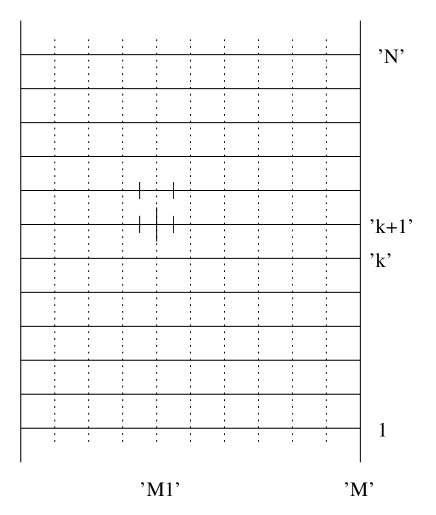
Figure 3: A mass insertion represented as a “short loop”.

Note that a cluster of four ghost links is missing in this diagram, and there are no extra momentum conserving delta functions. Thus the insertion will provide a factor of $1/M^{2}$. If we remember that on a fixed time slice the insertion can be placed on $M-1$ sites, we see that the net factor is $(M-1)/M^{2}\sim 1/M$ for the continuum limit $M\rightarrow\infty$. This is precisely the $M$ dependence required of a perturbative mass insertion: $e^{-a\mu^{2}/2Mm}\sim 1-(a/m)\mu^{2}/2M$. In the Ising spin representation of the sum over diagrams this mass insertion would be multiplied by the Ising spin factors $(1-s_{i}^{j-1})(1+s_{i}^{j})(1-s_{i}^{j+1})/8$:

$${\rm Mass~{}Term} = -{a\over m}\sum_{i,j}\left[(b_{i}^{j}-b_{i-1}^{j})(c_{i}^{j}-c_{i-1}^{j})+(b_{i+1}^{j}-b_{i}^{j})(c_{i+1}^{j}-c_{i}^{j})+\mu\sqrt{a\over 2m}b_{i}^{j}c_{i}^{j}\right.$$ (45)

$$\quad\left.+(b_{i}^{j+1}-b_{i-1}^{j+1})(c_{i}^{j+1}-c_{i-1}^{j+1})+(b_{i+1}^{j+1}-b_{i}^{j+1})(c_{i+1}^{j+1}-c_{i}^{j+1})-\mu\sqrt{a\over 2m}b_{i}^{j+1}c_{i}^{j+1}\right]$$

$$\hskip 113.81102pt\times{(1-s_{i}^{j-1})(1+s_{i}^{j})(1-s_{i}^{j+1})\over 8}.$$

Note that since we want the mass insertion to give a negative prefactor $-\mu^{2}$ we have used opposite signs in the two terms proportional to $\mu$.

If there are several fields with different mass, introducing a mass insertion into the bulk in this way would not be a local procedure since a whole strip must then change its mass simultaneously. Indeed, even if the mass were the same for two fields of different “flavor” it is clear that the flavor information must reside on the boundaries in order for flavor changing transitions to be local on the worldsheet. Thus in this case flavor dependent mass differences must also reside on the boundaries. This is certainly feasible: just use an insertion in which there is only one missing ghost link next to the boundary. This would provide a factor of $1/M$, which is correct, since there are not order $O(M)$ places to insert on a fixed time slice.

7 Dualities

It is interesting and amusing to compare the lattice world sheet we have set up to sum planar QFT with the lattice string formalism set up in [14] to sum planar open-string multi-loop diagrams. The two pictures are dual in almost every conceivable meaning carried by that word.

First of all the lattice string formalism uses transverse coordinates as basic variables while the QFT world sheet uses transverse momentum variables. Secondly, the basic variables satisfy Neumann boundary conditions in the lattice string theory but Dirichlet boundary conditions in the QFT. Thirdly, a loop in the lattice string formalism is described by a row of missing spatial links, whereas a loop on the QFT worldsheet is represented by a row of added temporal links. Finally the role of strong and weak coupling is reversed in the two pictures: at zero coupling every spatial link is present on the string worldsheet, but at zero coupling on the QFT worldsheet no temporal link is present. Conversely, at strong coupling a maximum number of spatial links are missing on the string world sheet, whereas a maximal number of temporal links are present on the QFT worldsheet.

8 Directions for Future Work

In this paper we have concentrated on the task of developing a world sheet description for the simplest possible matrix quantum field theory: a scalar theory with cubic interactions. When we turn to richer theories there are a number of technical problems that emerge in the application of our methods.

Consider first the simple complication of including several types (flavors) of field. If different fields couple to each other, a local worldsheet description requires that the “bits” of the different fields are the same “stuff”. Whatever differences there are must occur at the boundaries. This suggests a Chan-Paton factor approach to flavor as in open string theory.

When we move on to consider fields with spin, life gets more interesting. Do we put the spin variables only on the boundaries or can we give the bits spin degrees of freedom in such a way that the total spin carried by the strip is fixed by boundary values of these variables? At the moment both seem viable possibilities, but we do not delve into them here.

Finally, what about quartic interactions? Our methods obviously work well with cubic vertices, but how can we deal in a worldsheet local way with quartic vertices? One way, but hopefully not the only way, is to represent quartic vertices as a concatenation of a pair of cubic vertices, as was done for example in [12]. If this is to work the intermediate “pseudoparticle” that connects the two cubic vertices should not propagate very long. This can be arranged, for example, by giving the intermediary a huge mass. Such a scheme can be made to work, but we hope a more elegant approach will emerge from future research.

It is a clear challenge to bring all interesting planar quantum field theories into a worldsheet description along the lines proposed in this article. Much work still needs to be done.

Acknowledgments: This work was supported in part by the Department of Energy under Grants No. DE-FG02-97ER-41029 and DE-AC03-76SF00098, and in part by tne National Science Foundation Grant PHY-0098840. Also CBT acknowledges support from the Miller Institute for Basic Research in Science.

References

- [1] H. B. Nielsen and P. Olesen, Phys. Lett. 32B (1970) 203; B. Sakita and M. A. Virasoro, Phys. Rev. Lett. 24 (1970) 1146.
- [2] G. ’t Hooft, Nucl. Phys. B72 (1974) 461.
- [3] C. B. Thorn, Phys. Lett. 70B (1977) 85; Phys. Rev. D17 (1978) 1073.
- [4] K. Bardakci and S. Samuel, Phys. Rev. D16 (1977) 2500.
- [5] E. Brezin and V. A. Kazakov, Phys. Lett. 236B (1990) 144.
- [6] M. R. Douglas and S. H. Shenker, Nucl. Phys. B335 (1990) 635.
- [7] D. J. Gross and A. A. Migdal, Phys. Rev. Lett. 64 (1990) 127; Phys. Rev. Lett. 64 (1990) 717; Nucl. Phys. B340 (1990) 333. Phys. Rev. Lett. 64 (1990) 717.
- [8] J. M. Maldacena, Adv. Theor. Math. Phys. 2 (1998) 231-252, hep-th/9711200.
- [9] S. S. Gubser, I. R. Klebanov, and A. M. Polyakov, Phys. Lett. B428 (1998) 105, hep-th/9802109.
- [10] E. Witten, Adv. Theor. Math. Phys. 2 (1998) 253-291 hep-th/9802150.
- [11] W. Siegel, Int. Journ. of Mod. Phys. A13 (1998) 381.
- [12] K. Bering, J. S. Rozowsky and C. B. Thorn, Phys. Rev. D61 (2000) 045007, hep-th/9909141.
- [13] S. Mandelstam, Nucl. Phys. B64 (1973) 205; Phys. Lett. 46B (1973) 447; Nucl. Phys. B69 (1974) 77; see also his lectures in Unified String Theories, ed. M. Green and D. Gross (World Scientific) 1986.
- [14] R. Giles and C. B. Thorn, Phys. Rev. D16 (1977) 366.
- [15] C. B. Thorn, Phys. Rev. D59 (1999) 025005, hep-th/9807151.
- [16] P. Hořava, ”Topological Strings and QCD in Two Dimensions,” hep-th/9311156; Nucl. Phys.B463(1996),238-286, hep-th/9507060; JHEP 9901(1999)016,1999; hep-th/9811028.
- [17] P. Goddard, J. Goldstone, C. Rebbi, and C. B. Thorn, Nucl. Phys. B56 (1973) 109.