Vacuum Stress Tensor of a Scalar Field
in a Rectangular Waveguide

R.B. $Rodrigues^{a,}$, N.F. $Svaiter^{a,}$ and R.D.M. De $Paola^{b,}$
^aCentro Brasileiro de Pesquisas Fisicas-CBPF

Rua Dr. Xavier Sigaud 150, Rio de Janeiro, RJ, 22290-180, Brazil

^bInstituto de Ciências - Escola Federal de Engenharia de Itajubá

Av. BPS 1303 Pinheirinho, 37500-903, Itajubá, MG - Brazil

Abstract

Using the heat kernel method and the analytic continuation of the zeta function, we calculate the canonical and improved vacuum stress tensors, $\left\langle T_{\mu\nu}(\vec{x})\right\rangle$ and $\left\langle\Theta_{\mu\nu}(\vec{x})\right\rangle$, associated with a massless scalar field confined in the interior of an infinitely long rectangular waveguide. The local depence of the renormalized energy for two special configurations when the total energy is positive and negative are presented using $\left\langle T_{00}(\vec{x})\right\rangle$ and $\left\langle\Theta_{00}(\vec{x})\right\rangle$. From the stress tensors we obtain the local Casimir forces in all walls by introducing a particular external configuration. It is shown that this external configuration cannot give account of the edge divergences of the local forces. The local form of the forces is obtained for three special configurations.

1 Introduction

In a previous paper, the one-loop renormalization of the anisotropic scalar model was performed, assuming that the fields were defined in a d-dimensional Euclidean space where the first $d-1$ coordinates are unbounded, while the last one lies in the interval $[0,L]$ [1]. The authors analysed the vacuum activity of massive scalar fields assuming different boundary conditions on the plates, namely Dirichlet-Dirichlet $(D-D)$ boundary conditions and also Neumann-Neumann $(N-N)$ boundary conditions. They obtained two different results. The first one has been obtained previously by many authors, and is the fact that to renormalize the theory we have to introduce counterterms as surface interactions. The second one is the fact that the tadpole graph for $DD$ and for $NN$ have the same $z$ dependent part in modulus but with opposite signs. This second result has been obtained by DeWitt [2] and also Deutsch and Candelas [3]. In ref.[1], the authors also investigated the relevance of this fact to eliminate the surface divergences.

More than thirty years ago, the local version of the Casimir original problem was performed by Brown and Maclay [4]. They obtained a constant stress-energy tensor due to the cancelation of the electric and magnetic sectors, showing the uniformity of the vacuum of the electromagnetic field for this configuration. The result is due in part to the particular field involved and also to the simplicity of the parallel plane geometry. A similar cancelation can be arranged for the scalar field by computing the improved stress-energy tensor, but in a more complicated rectangular geometry with the presence of edges and corners (e.g. within a rectangular waveguide), we expect an answer strongly non-uniform. The aim of this paper is to generalize part of the results of Fosco and Svaiter [1], introducing edges in the domain where the fields are defined, calculating the renormalized stress-energy tensor of a massless scalar field in an infinitely long rectangular waveguide. As was stressed by Maclay, geometries with corners present special problems with respect to vacuum energy; nevertheless these issues have received little attention in the literature [5]. It is commonly accepted that, the understanding of the renormalization of the stress-energy tensor of quantum fields in the presence of classical boundaries should throw light on the more difficult case, where there is the added complication of local curvature effects [6].

It is well known that there are two quantities which might be expected to correspond to the total renormalized energy of quantum fields [3]. The first one is called the mode sum energy and its definition is

$$\left<E\right>_{ren}^{mode}=\int_{0}^{\infty}d\omega\,\frac{1}{2}\omega[N(\omega)-N_{0}(\omega)],$$ (1)

where $\frac{1}{2}\omega$ is the zero point energy for each mode, $N(\omega)d\omega$ is the number of modes with frequencies between $\omega$ and $\omega+d\omega$ in the presence of boundaries and $N_{0}(\omega)d\omega$ is the corresponding quantity evaluated in empty space. The above equation gives the renormalized sum of the zero point energy for each mode. The second one is the volume integral of the renormalized energy density $\left<E\right>_{ren}^{vol}$ obtained by the Green’s function method [4, 9]. A recent investigation of $\left<E\right>_{ren}^{mode}$ in rectangular geometries was given by Svaiter and colaborators [10, 11]. A seminal paper studying this kind of geometry was made by Ambjorn and Wolfram [12], and more recently Milton and Ng studied the Casimir effect in $(2+1)$ Maxwell-Chern-Simons electrodynamics in a rectangular domain [13]. Since these definitions deal with integrated quantities, surface divergence problems do not appear in the calculations. Although global effects are more accessible to experiments, it is quite important to understand how the global effect is obtained from the local version. This issue has recently been studied by Actor and Bender [7, 8].

In ref. [7] the author studied the use of the zeta function method to find the effective action associated with a scalar field defined in the interior of the infinitely long waveguide, while in ref. [8] the authors use the same method to compute the stress-energy tensor for various rectangular geometries. Using the relation between the local force density and the discontinuity of the stress-energy tensor across the boundaries, they computed the local Casimir forces, which exhibited strong position dependence.

In this paper we are interested in calculating local quantities in the presence of surfaces and edges. As was stressed by Dowker and Kennedy [14] and also Actor and Bender [8], to study the local problem in the infinitely long rectangular waveguide, it is necessary to present the local form of the analytic continuation of the local zeta function in the rectangle. Note that our choice of a rectangular cavity is related to the fact that the modes of the field in this geometric configuration are well known and an exact calculation can be done.

The organization of the paper is the following: In section II a brief review of the zeta function method is presented. In section III we calculate the vacuum expectation value of the canonical and improved stress-energy tensors associated with a massless scalar field using the zeta function method in the infinitely long rectangular waveguide. We also show in section III the relation that exists between the local version and the global version of the Casimir energy for the waveguide. In section IV, we use the results of the previous section to compute the local forces. In order to do this we introduce an external configuration (such that the interior region is the waveguide) for which the components of the stress-tensors are known everywhere. Conclusions are given in section V. In this paper we use $\hbar=c=1$.

2 The canonical and improved stress tensors and the zeta function method

In this section we will describe the basic procedure to compute the renormalized vacuum expectation value of the stress-energy tensor for a real scalar field. Our aproach will be based on the zeta function method.

For a real scalar field defined in a four dimensional spacetime, distorted by static boundaries, we can use the Fourier standard expansion

$$\phi(x)=\sum_{n}\frac{1}{\sqrt{2\omega_{n}}}\left[a_{n}e^{-ix_{0}\omega_{n}}\phi_{n}(\vec{x})+a_{n}^{\dagger}e^{ix_{0}\omega_{n}}\phi_{n}^{*}(\vec{x})\right]\ .$$ (2)

Assuming that the manifold is static, i.e., that it possesses a timelike Killing vector field, it is possible to show that there is a complete set of spatial modes $\left\{\phi_{n}(\vec{x})\right\}$ satisfying a Schrödinger-like equation

$$-\Delta\phi_{n}(\vec{x})=\omega_{n}^{2}\phi_{n}(\vec{x}),$$ (3)

where over these modes we will impose certain boundary conditions. Here we are concerned only with Dirichlet boundary conditions, although the generalization to Neumann boundary conditions is straightfoward. Since the set of modes $\phi_{n}(\vec{x})$ are orthonormal and complete, one then readily verifies that the equal-time canonical commutation relations imply the usual commutation relation between annihilation and creation operators of the quanta of the field.

The main point of interest for us will be the renormalized stress-energy tensor of the scalar field confined in the interior of the rectangular infinitely long waveguide. The canonical and improved stress tensors of a real massless scalar field are given by

$$T_{\mu\nu}(x)=\frac{1}{2}\left[\partial_{\mu}\phi\,\partial_{\nu}\phi+\partial_{\nu}\phi\,\partial_{\mu}\phi-\eta_{\mu\nu}\partial_{\alpha}\phi\partial^{\alpha}\phi\right]$$ (4)

and

$$\Theta_{\mu\nu}(x)=\frac{1}{3}\left[\partial_{\mu}\phi\,\partial_{\nu}\phi+\partial_{\nu}\phi\,\partial_{\mu}\phi-\frac{1}{2}\left(\phi\partial_{\mu}\,\partial_{\nu}\phi+\partial_{\mu}\partial_{\nu}\phi.\phi+\eta_{\mu\nu}\partial_{\alpha}\phi\partial^{\alpha}\phi\right)\right],$$ (5)

where $\eta_{\mu\nu}$ is the Minkowski metric. One way to write the vacuum expectation value of $T_{\mu\nu}(x)$ using eq.(4) is

$$\left\langle T_{\mu\nu}(x)\right\rangle=\lim_{y\rightarrow x}\frac{1}{2}\left[\frac{\partial}{\partial x^{\mu}}\frac{\partial}{\partial y^{\nu}}+\frac{\partial}{\partial x^{\nu}}\frac{\partial}{\partial y^{\mu}}-\eta_{\mu\nu}\frac{\partial}{\partial x^{\alpha}}\frac{\partial}{\partial y_{\alpha}}\right]\left\langle\phi(x)\phi(y)\right\rangle,$$ (6)

where $\left\langle\phi(x)\phi(y)\right\rangle$ is the vacuum expectation value of the product of the fields in two different points. (An equivalent relation exists for $\left<\Theta_{\mu\nu}\right>$.) Using the commutation relations between annihilation and creation operators, the quantity $\left\langle\phi(x)\phi(y)\right\rangle$ in eq.(6), can be written as

$$\left\langle\phi(x)\phi(y)\right\rangle=\sum_{n}\frac{1}{2\omega_{n}}\exp(-i\left(x_{0}-y_{0}\right)\omega_{n})\phi_{n}(\vec{x})\phi_{n}^{*}(\vec{y})\ .$$ (7)

It is clear that $\left\langle T_{\mu\nu}(x)\right\rangle$ can be obtained from the bilocal sum given by eq.(7). The bilocal (spectral) sum in eq.(7) diverges and needs a regularization and renormalization procedure. A convenient method is to set $x_{0}=y_{0}$ and replace $\omega_{n}^{-1}$ in eq.(7) by $\omega_{n}^{-2s}$ with $s$ complex, initially holding for $Re(s)>0$ and sufficiently large to guarantee convergence even for $\vec{x}=\vec{y}$ , followed by analytic continuation in $s$.

Let us work with a compact manifold $M$ with or without boundaries. The diagonal zeta function associated with some elliptic, semi-positive and self-adjoint differential operator $D$ will be defined by $\zeta(s|D)$. Let $\phi_{n}(x)$ and $\lambda_{n}$ be the spectral decomposition of $D$ in a complete normal set of eigenfunctions $\phi_{n}(x)$ with eigenvalues $\lambda_{n}$, i.e.

$$D\phi_{n}(x)=\lambda_{n}\phi_{n}(x)$$ (8)

where $\phi_{n}(x)=\left\langle x|n\right\rangle$. Since the eigenfuctions $\phi_{n}(x)$ form a complete and normal set it is possible to define the generalized zeta operator associated with $D$ as

$$\hat{\zeta}(s|D)=\mu^{2s}\sum_{n}^{\prime}\frac{\left|n\rangle\langle n\right|}{\lambda_{n}^{s}},$$ (9)

where we introduce the parameter $\mu$ with dimensions of mass in order to have a dimensionless quantity raised to a complex power and the prime sign indicates that the zero eigenvalue of $D$ must be ommited. The generalized zeta function associated with the operator $D$ is defined by

$$\zeta(s|D)=\mu^{2s}\int_{M}d\gamma(x)\left\langle x|D^{-s}|x\right\rangle,$$ (10)

where $d\gamma(x)$ is the measure on $M$. We have then to consider the bilocal zeta function

$$\zeta\left(s\mid\vec{x},\vec{y}\right)=\mu^{2s}\sum_{n}\left(\omega_{n}^{2}\right)^{-s}\phi_{n}(\vec{x})\phi_{n}^{*}(\vec{y}),$$ (11)

which has abscissa of convergence $Re(s)=\frac{3}{2}$. Since the modes $\phi_{n}(\vec{x})$ form an orthonormal set then the passage from the local to the more familiar global zeta function is straightforward for $Re(s)>\frac{3}{2}$. This can be done integrating the bilocal zeta function, i.e.

$$\zeta(s)=\mu^{2s}\int d\gamma(x)\,\zeta\left(s\mid\vec{x},\vec{x}\right)=\mu^{2s}\sum_{n}\left(\omega_{n}^{2}\right)^{-s},\quad Re(s)>\frac{3}{2}.$$ (12)

A careful analysis of the analytic extension of the global zeta function associated with some differential operator defined in compact manifold with or without boundaries can be found in ref. [15]. Going back to the local case in the analytic extension of the local zeta function to the whole complex plane (to the region $Re(s)<\frac{3}{2}$), it will appear poles related with the geometry of the manifold. For sake of simplicity we will omit the $\mu$ factor in the following.

The function given by eq.(11) is related to the heat kernel by a Mellin transform

$$\zeta\left(s\mid\vec{x},\vec{y}\right)=\frac{1}{\Gamma(s)}\int_{0}^{\infty}dt\,t^{s-1}K\left(t\mid\vec{x},\vec{y}\right)$$ (13)

where

$$K\left(t\mid\vec{x},\vec{y}\right)=\sum_{n}e^{-t\omega_{n}^{2}}\phi_{n}(\vec{x})\phi_{n}^{*}(\vec{y})$$ (14)

is the heat kernel satisfying the same boundary conditions that we choose to the complete set of modes $\phi_{n}(\vec{x})$. It is possible to express the vacuum expectation value of the canonical stress tensor given by eq.(6) in terms of the modes $\phi_{n}$ and also the frequencies $\omega_{n}$. We have

$$\left\langle T_{00}(x)\right\rangle=\frac{1}{4}\sum_{n}\omega_{n}\left|\phi_{n}\right|^{2}+\frac{1}{4}\sum_{n}\frac{1}{\omega_{n}}\left|\vec{\nabla}\phi_{n}\right|^{2}$$ (15)

and

$$\left\langle T_{ii}(x)\right\rangle=\frac{1}{4}\sum_{n}\omega_{n}\left|\phi_{n}\right|^{2}-\frac{1}{4}\sum_{n}\frac{1}{\omega_{n}}\left|\vec{\nabla}\phi_{n}\right|^{2}+\frac{1}{2}\sum_{n}\frac{1}{\omega_{n}}\left|\partial_{i}\phi_{n}\right|^{2}$$ (16)

$i$ not summed. It is easy to see that for $\phi_{n}$ real and for plane waves

$$\left\langle T_{0i}(x)\right\rangle=0$$ (17)

and finally

$$\left\langle T_{ij}(x)\right\rangle=\frac{1}{4}\sum_{n}\frac{1}{\omega_{n}}\left[\partial_{i}\phi_{n}\partial_{j}\phi_{n}^{*}+\partial_{j}\phi_{n}\partial_{i}\phi_{n}^{*}\right]\quad i\neq j\ .$$ (18)

For the improved stress tensor we have:

$$\left\langle\Theta_{00}(x)\right\rangle=\frac{5}{12}\sum_{n}\omega_{n}\left|\phi_{n}\right|^{2}+\frac{1}{12}\sum_{n}\frac{1}{\omega_{n}}\left|\vec{\nabla}\phi_{n}\right|^{2}$$ (19)

$$\left\langle\Theta_{ii}(x)\right\rangle=\frac{1}{3}\sum_{n}\frac{1}{\omega_{n}}\left|\partial_{i}\phi_{n}\right|^{2}+\frac{1}{12}\sum_{n}\omega_{n}\left|\phi_{n}\right|^{2}-\frac{1}{12}\sum_{n}\frac{1}{\omega_{n}}\left|\vec{\nabla}\phi_{n}\right|^{2}-\frac{1}{12}\sum_{n}\frac{1}{\omega_{n}}\left[\phi_{n}\partial_{i}^{2}\phi_{n}^{*}+\left(\partial_{i}^{2}\phi_{n}\right)\phi_{n}^{*}\right]$$ (20)

$i$ not summed,

$$\left\langle\Theta_{0i}(x)\right\rangle=\left\langle T_{0i}(x)\right\rangle=0\,,$$ (21)

$$\left\langle\Theta_{ij}(x)\right\rangle=\frac{1}{6}\sum_{n}\frac{1}{\omega_{n}}\left[\partial_{i}\phi_{n}\partial_{j}\phi_{n}^{*}+\partial_{j}\phi_{n}\partial_{i}\phi_{n}^{*}\right]-\frac{1}{12}\sum_{n}\frac{1}{\omega_{n}}\left[\phi_{n}\partial_{i}\partial_{j}\phi_{n}^{*}+\left(\partial_{i}\partial_{j}\phi_{n}\right)\phi_{n}^{*}\right]\quad i\neq j\ .$$ (22)

In the next section we will identify the divergences and the finite parts that appear in the vacuum expectation value of the canonical and the improved stress tensors of a real massless scalar field satisfying Dirichlet boundary conditions in all walls of an infinitely long rectangular waveguide.

3 Canonical and improved stress-energy tensor of a massless scalar field confined within a rectangular waveguide

In this section we will apply the local zeta function method to calculate the renormalized vacuum expectation values of the canonical and improved stress-energy tensors of a massless scalar field confined within an infinitely long rectangular waveguide. Let the waveguide be oriented along the $x_{3}$ axis in such a way that the field is defined free in the region

$$\Omega={{\bf x}\equiv(x_{1},x_{2},x_{3}):0<x_{1}<a,\quad 0<x_{2}<b}\subset{\bf R}^{3},$$ (23)

with Dirichlet boundary conditions at $x_{1}=0$ and $x_{1}=a$ and also $x_{2}=0$ and $x_{2}=b$. The spatial modes are given by:

$$\phi_{m_{1},m_{2}}\left(\vec{x}\right)=\left(\frac{4}{ab}\right)^{\frac{1}{2}}\sin\frac{m_{1}\pi x_{1}}{a}\sin\frac{m_{2}\pi x_{2}}{b}\frac{1}{\sqrt{2\pi}}e^{ik_{3}x_{3}},$$ (24)

with $m_{1,2}=1,2,3,...$ and $-\infty<k_{3}<\infty$. The eigenvalues are given by

$$\omega_{n}^{2}=\left(\left(\frac{m_{1}\pi}{a}\right)^{2}+\left(\frac{m_{2}\pi}{b}\right)^{2}+k_{3}^{2}\right),$$ (25)

where $n$ denotes the collective indices $(m_{1},m_{2},k_{3})$. Substituting eq.(24) in eq.(14) the heat-kernel can be written as:

$$K\left(t\mid\vec{x},\vec{y}\right) = \sum_{m}e^{-t\omega_{m}^{2}}\phi_{m}\left(\vec{x}\right)\phi_{m}(\vec{y})$$ (26)

$$= \frac{1}{2\pi}\left(\frac{4}{ab}\right)\int_{-\infty}^{\infty}dk_{3}\sum_{m_{1},m_{2}=1}^{\infty}\exp\left\{-t\left[\left(\frac{m_{1}\pi}{a}\right)^{2}+\left(\frac{m_{2}\pi}{b}\right)^{2}+\left(k_{3}\right)^{2}\right]\right\}$$

$$\times\sin(\frac{m_{1}\pi x_{1}}{a})\sin(\frac{m_{2}\pi x_{2}}{b})\sin(\frac{m_{1}\pi y_{1}}{a})\sin(\frac{m_{2}\pi y_{2}}{b})e^{ik_{3}\left(x_{3}-y_{3}\right)}.$$

The free spacetime part can be integrated imediately:

$$\frac{1}{2\pi}\int dk_{3}\,e^{-t\left(k_{3}\right)^{2}}e^{ik_{3}\left(x_{3}-y_{3}\right)}=\left(4\pi t\right)^{-\frac{1}{2}}\exp\left[-\frac{\left(x_{3}-y_{3}\right)^{2}}{4t}\right],$$ (27)

yielding

$$K\left(t\mid\vec{x},\vec{y}\right) = \frac{4}{ab}\left(4\pi t\right)^{-\frac{1}{2}}\exp\left[-\frac{\left(x_{3}-y_{3}\right)^{2}}{4t}\right]$$ (28)

$$\times\sum_{m_{1}=1}^{\infty}\exp\left[-t\left(\frac{m_{1}\pi}{a}\right)^{2}\right]\sin(\frac{m_{1}\pi x_{1}}{a})\sin(\frac{m_{1}\pi y_{1}}{a})$$

$$\times\sum_{m_{2}=1}^{\infty}\exp\left[-t\left(\frac{m_{2}\pi}{b}\right)^{2}\right]\sin(\frac{m_{2}\pi x_{2}}{b})\sin(\frac{m_{2}\pi y_{2}}{b}).$$

Using trigonometric identities and also the Jacobi $\theta$-function identity

$$\sum_{m=1}^{\infty}\exp(-m^{2}x)\cos(m2\pi h)=-\frac{1}{2}+\sqrt{\frac{\pi}{4x}}\sum_{n=-\infty}^{\infty}\exp\left[-(n+h)^{2}\frac{\pi^{2}}{x}\right]$$ (29)

one finds to the heat-kernel

$$K\left(t\mid\vec{x},\vec{y}\right) = (4\pi t)^{-\frac{3}{2}}\exp\left[-\frac{\left(x_{3}-y_{3}\right)^{2}}{4t}\right]$$ (30)

$$\times\sum_{n_{1}=-\infty}^{\infty}\left\{\exp\left[\frac{-\left[2n_{1}a+(x_{1}-y_{1})\right]^{2}}{4t}\right]-\exp\left[\frac{-\left[2n_{1}a+(x_{1}+y_{1})\right]^{2}}{4t}\right]\right\}$$

$$\times\sum_{n_{2}=-\infty}^{\infty}\left\{\exp\left[\frac{-\left[2n_{2}b+(x_{2}-y_{2})\right]^{2}}{4t}\right]-\exp\left[\frac{-\left[2n_{2}b+(x_{2}+y_{2})\right]^{2}}{4t}\right]\right\}.$$

As we discussed before to find the bilocal zeta function we need to perform the Mellin transform of the heat-kernel given by eq.(30). All terms of eq.(30) can be integrated using [16]

$$\int_{0}^{\infty}dt\,t^{s-\frac{5}{2}}\exp(-\frac{A}{t})=A^{s-\frac{3}{2}}\Gamma(\frac{3}{2}-s).$$ (31)

After a straightforward calculation we have

$$\zeta\left(s\mid\vec{x},\vec{y}\right)=\frac{\Gamma(\frac{3}{2}-s)}{\left(4\pi\right)^{\frac{3}{2}}\Gamma(s)}\sum_{n_{1},n_{2}=-\infty}^{\infty}\left(Z_{1}+Z_{2}+Z_{3}+Z_{4}\right),$$ (32)

where $Z_{j}=Z_{j}(n_{1},n_{2},\vec{x},\vec{y}),\quad j=1,2,3,4$, are given by

$$Z_{1} = \left[\left(n_{1}a+\frac{(x_{1}-y_{1})}{2}\right)^{2}+\left(n_{2}b+\frac{(x_{2}-y_{2})}{2}\right)^{2}+(\frac{x_{3}-y_{3}}{2})^{2}\right]^{s-\frac{3}{2}}$$ (33)

$$Z_{2} = -\left[\left(n_{1}a+\frac{(x_{1}-y_{1})}{2}\right)^{2}+\left(n_{2}b+\frac{(x_{2}+y_{2})}{2}\right)^{2}+(\frac{x_{3}-y_{3}}{2})^{2}\right]^{s-\frac{3}{2}}$$ (34)

$$Z_{3} = -\left[\left(n_{1}a+\frac{(x_{1}+y_{1})}{2}\right)^{2}+\left(n_{2}b+\frac{(x_{2}-y_{2})}{2}\right)^{2}+(\frac{x_{3}-y_{3}}{2})^{2}\right]^{s-\frac{3}{2}}$$ (35)

$$Z_{4} = \left[\left(n_{1}a+\frac{(x_{1}+y_{1})}{2}\right)^{2}+\left(n_{2}b+\frac{(x_{2}+y_{2})}{2}\right)^{2}+(\frac{x_{3}-y_{3}}{2})^{2}\right]^{s-\frac{3}{2}}.$$ (36)

We see that divergences appear in the local zeta function $\zeta(s\mid\vec{x},\vec{y})$ in the limit $\vec{y}\rightarrow\vec{x}.$ We note that $\zeta(s\mid\vec{x},\vec{x})$ has surface divergences when $Re(s)<\frac{3}{2}$ . The term $Z_{2}\left(0,0,\vec{x},\vec{x}\right)=\left(x_{2}\right)^{2s-3}$, for example, diverges when $x_{2}\rightarrow 0$ in this case.

In order to calculate the components of $\left\langle T_{\mu\nu}(\vec{x})\right\rangle$ we have to evaluate the mode sums given by eqs.(15)-(18). One then readily verifies that

$$\sum_{n}\omega_{n}\left|\phi_{n}\right|^{2}=\zeta(s=-\frac{1}{2}\mid\vec{x},\vec{x})=-\frac{1}{16\pi^{2}}F_{0}(\vec{x}),$$ (37)

where the expression for $F_{0}(\vec{x})$ is given by

$$F_{0}(\vec{x}) = \sum_{n_{1},n_{2}=-\infty}^{\infty}\left[(n_{1}a)^{2}+(n_{2}b)^{2}\right]^{-2}+$$ (38)

$$\hskip 28.45274pt-\left[(n_{1}a)^{2}+\left(n_{2}b+x_{2}\right)^{2}\right]^{-2}+$$

$$\hskip 28.45274pt-\left[\left(n_{1}a+x_{1}\right)^{2}+\left(n_{2}b\right)^{2}\right]^{-2}+$$

$$\hskip 28.45274pt+\left[\left(n_{1}a+x_{1}\right)^{2}+\left(n_{2}b+x_{2}\right)^{2}\right]^{-2}.$$

The other terms that we need are given by:

$$\sum_{n}\frac{1}{\omega_{n}}|\partial_{i}\phi_{n}|^{2}=\lim_{\vec{y}\rightarrow\vec{x}}\frac{\partial}{\partial x^{i}}\frac{\partial}{\partial y^{i}}\zeta(s=\frac{1}{2}\mid\vec{x},\vec{y}).$$ (39)

Substituting eq.(32) in eq.(39) for $i=1,$ we have:

$$\sum_{n}\frac{1}{\omega_{n}}\left|\partial_{1}\phi_{n}\right|^{2}=-\frac{1}{4\pi^{2}}D_{1}(\vec{x})+\frac{1}{16\pi^{2}}F_{1}(\vec{x}),$$ (40)

where the functions $D_{1}(\vec{x})$ and F${}_{1}\left(\vec{x}\right)$ are defined by

$$D_{1}(\vec{x}) = \sum_{n_{1},n_{2}=-\infty}^{\infty}\left[(n_{1}a)^{2}+(n_{2}b)^{2}\right]^{-3}\left[n_{1}a\right]^{2}$$ (41)

$$\hskip 28.45274pt-\left[(n_{1}a)^{2}+\left(n_{2}b+x_{2}\right)^{2}\right]^{-3}\left[n_{1}a\right]^{2}+$$

$$\hskip 28.45274pt+\left[\left(n_{1}a+x_{1}\right)^{2}+\left(n_{2}b\right)^{2}\right]^{-3}\left[n_{1}a+x_{1}\right]^{2}+$$

$$\hskip 28.45274pt-\left[\left(n_{1}a+x_{1}\right)^{2}+\left(n_{2}b+x_{2}\right)^{2}\right]^{-3}\left[n_{1}a+x_{1}\right]^{2}$$

and

$$F_{1}(\vec{x}) = \sum_{n_{1},n_{2}=-\infty}^{\infty}\left[(n_{1}a)^{2}+(n_{2}b)^{2}\right]^{-2}+$$ (42)

$$\hskip 28.45274pt-\left[(n_{1}a)^{2}+\left(n_{2}b+x_{2}\right)^{2}\right]^{-2}+$$

$$\hskip 28.45274pt+\left[\left(n_{1}a+x_{1}\right)^{2}+\left(n_{2}b\right)^{2}\right]^{-2}+$$

$$\hskip 28.45274pt-\left[\left(n_{1}a+x_{1}\right)^{2}+\left(n_{2}b+x_{2}\right)^{2}\right]^{-2}.$$

For $i=2$,

$$\sum_{n}\frac{1}{\omega_{n}}\left|\partial_{2}\phi_{n}\right|^{2}=-\frac{1}{4\pi^{2}}D_{2}(\vec{x})+\frac{1}{16\pi^{2}}F_{2}(\vec{x}),$$ (43)

where the functions $D_{2}(\vec{x})$ and $F_{2}(\vec{x})$ are defined by

$$D_{2}(\vec{x}) = \sum_{n_{1},n_{2}=-\infty}^{\infty}\left[(n_{1}a)^{2}+(n_{2}b)^{2}\right]^{-3}\left[n_{2}b\right]^{2}$$ (44)

$$\hskip 28.45274pt+\left[(n_{1}a)^{2}+\left(n_{2}b+x_{2}\right)^{2}\right]^{-3}\left[n_{2}b+x_{2}\right]^{2}+$$

$$\hskip 28.45274pt-\left[\left(n_{1}a+x_{1}\right)^{2}+\left(n_{2}b\right)^{2}\right]^{-3}\left[n_{2}b\right]^{2}+$$

$$\hskip 28.45274pt-\left[\left(n_{1}a+x_{1}\right)^{2}+\left(n_{2}b+x_{2}\right)^{2}\right]^{-3}\left[n_{2}b+x_{2}\right]^{2}$$

and

$$F_{2}(\vec{x}) = \sum_{n_{1},n_{2}=-\infty}^{\infty}\left[(n_{1}a)^{2}+(n_{2}b)^{2}\right]^{-2}+$$ (45)

$$\hskip 28.45274pt+\left[(n_{1}a)^{2}+\left(n_{2}b+x_{2}\right)^{2}\right]^{-2}+$$

$$\hskip 28.45274pt-\left[\left(n_{1}a+x_{1}\right)^{2}+\left(n_{2}b\right)^{2}\right]^{-2}+$$

$$\hskip 28.45274pt-\left[\left(n_{1}a+x_{1}\right)^{2}+\left(n_{2}b+x_{2}\right)^{2}\right]^{-2}.$$

For $i=3$

$$\sum_{n}\frac{1}{\omega_{n}}\left|\partial_{3}\phi_{n}\right|^{2}=\frac{1}{16\pi^{2}}F_{0}(\vec{x}).$$ (46)

We still need to calculate

$$\sum_{n}\frac{1}{\omega_{n}}\partial_{i}\phi_{n}\partial_{j}\phi_{n}^{*}=\lim_{\vec{y}\rightarrow\vec{x}}\frac{\partial}{\partial x^{i}}\frac{\partial}{\partial y^{i}}\zeta(s=\frac{1}{2}\mid\vec{x},\vec{y}).$$ (47)

For i=2 and j=1, we have

$$\sum_{n}\frac{1}{\omega_{n}}\partial_{2}\phi_{n}\partial_{1}\phi_{n}^{*}=\sum_{n}\frac{1}{\omega_{n}}\partial_{1}\phi_{n}\partial_{2}\phi_{n}^{*}=-\frac{F_{21}(\vec{x})}{4\pi^{2}}\,,$$ (48)

where the function $F_{21}(\vec{x})$ is defined by

$$F_{21}(\vec{x}) = \sum_{n_{1},n_{2}=-\infty}^{\infty}\left[(n_{1}a)^{2}+(n_{2}b)^{2}\right]^{-3}\left[n_{2}b\right]\left[n_{1}a\right]+$$ (49)

$$\hskip 28.45274pt-\left[\left(n_{2}b+x_{2}\right)^{2}+\left(n_{1}a\right)^{2}\right]^{-3}\left[n_{2}b+x_{2}\right]\left[n_{1}a\right]+$$

$$\hskip 28.45274pt+\left[\left(n_{1}a+x_{1}\right)^{2}+\left(n_{2}b\right)^{2}\right]^{-3}\left[n_{1}a+x_{1}\right]\left[n_{2}b\right]+$$

$$\hskip 28.45274pt-\left[\left(n_{1}a+x_{1}\right)^{2}+\left(n_{2}b+x_{2}\right)^{2}\right]^{-3}\left[n_{1}a+x_{1}\right]\left[n_{2}b+x_{2}\right]$$

$$= -\sum_{n_{1},n_{2}=-\infty}^{\infty}\left[\left(n_{1}a+x_{1}\right)^{2}+\left(n_{2}b+x_{2}\right)^{2}\right]^{-3}\left[n_{1}a+x_{1}\right]\left[n_{2}b+x_{2}\right],$$

because the first three summands are odd in one index.

For i=3 and j=1 and for i=3 and j=2, we have

$$\sum_{n}\frac{1}{\omega_{n}}\partial_{3}\phi_{n}\partial_{1}\phi_{n}^{*}=\sum_{n}\frac{1}{\omega_{n}}\partial_{3}\phi_{n}\partial_{2}\phi_{n}^{*}=0.$$ (50)

To obtain the components of the improved stress tensor we need to calculate

$$\sum_{n}\frac{1}{\omega_{n}}\phi_{n}\partial_{i}^{2}\phi_{n}^{*}=\sum_{n}\frac{1}{\omega_{n}}\left(\partial_{i}^{2}\phi_{n}\right)\phi_{n}^{*}=\lim_{\vec{y}\rightarrow\vec{x}}\left(\frac{\partial}{\partial y^{i}}\right)^{2}\zeta(s=\frac{1}{2}\mid\vec{x},\vec{y}).$$ (51)

For $i=1$

$$\sum_{n}\frac{1}{\omega_{n}}\phi_{n}\partial_{1}^{2}\phi_{n}^{*}=\frac{1}{4\pi^{2}}D_{11}(\vec{x})-\frac{1}{16\pi^{2}}F_{0}(\vec{x})\,,$$ (52)

where the function $D_{11}(\vec{x})$ is defined by

$$D_{11}(\vec{x}) = \sum_{n_{1},n_{2}=-\infty}^{\infty}\{\left[(n_{1}a)^{2}+(n_{2}b)^{2}\right]^{-3}\left[n_{1}a\right]^{2}$$ (53)

$$\hskip 28.45274pt-\left[(n_{1}a)^{2}+\left(n_{2}b+x_{2}\right)^{2}\right]^{-3}\left[n_{1}a\right]^{2}+$$

$$\hskip 28.45274pt-\left[\left(n_{1}a+x_{1}\right)^{2}+\left(n_{2}b\right)^{2}\right]^{-3}\left[n_{1}a+x_{1}\right]^{2}+$$

$$\hskip 28.45274pt+\left[\left(n_{1}a+x_{1}\right)^{2}+\left(n_{2}b+x_{2}\right)^{2}\right]^{-3}\left[n_{1}a+x_{1}\right]^{2}\}.$$

For $i=2$

$$\sum_{n}\frac{1}{\omega_{n}}\phi_{n}\partial_{2}^{2}\phi_{n}^{*}=\frac{1}{4\pi^{2}}D_{22}(\vec{x})-\frac{1}{16\pi^{2}}F_{0}(\vec{x}),$$ (54)

where the function $D_{22}(\vec{x})$ can be obtained from $D_{11}(\vec{x})$ with the change $x_{1}\leftrightarrow x_{2}$ and $n_{1}a\leftrightarrow n_{2}b$. For $i=3$

$$\sum_{n}\frac{1}{\omega_{n}}\phi_{n}\partial_{3}^{2}\phi_{n}^{*}=-\frac{1}{16\pi^{2}}F_{0}(\vec{x}).$$ (55)

Finally

$$\sum_{n}\frac{1}{\omega_{n}}\phi_{n}\partial_{i}\partial_{j}\phi_{n}^{*}=\lim_{\vec{y}\rightarrow\vec{x}}\frac{\partial}{\partial y^{i}}\frac{\partial}{\partial y^{j}}\zeta(s=\frac{1}{2}\mid\vec{x},\vec{y}).$$ (56)

For $i=1$ and $j=2$

$$\sum_{n}\frac{1}{\omega_{n}}\phi_{n}\partial_{1}\partial_{2}\phi_{n}^{*}=\sum_{n}\frac{1}{\omega_{n}}\phi_{n}\partial_{2}\partial_{1}\phi_{n}^{*}=-\frac{F_{12}(\vec{x})}{4\pi^{2}}.$$ (57)

Substituting the results of eqs.(37), (40), (43), (46), (48) and (50) in eqs. (15-18), we obtain:

$$\left\langle T_{00}(\vec{x})\right\rangle = -\frac{1}{16\pi^{2}}\left(D_{1}(\vec{x})+D_{2}(\vec{x})\right)+\frac{1}{64\pi^{2}}\left(F_{1}(\vec{x})+F_{2}(\vec{x})\right)$$ (58)

$$= \left\langle T_{00}(\vec{x})\right\rangle_{B}+\left\langle T_{00}(\vec{x})\right\rangle_{F},$$

where B and F mean the boundary divergent and finite part respectively. In explicit form:

$$\left\langle T_{00}(\vec{x})\right\rangle_{B} = \frac{1}{32\pi^{2}}\{\left[\left(x_{1}\right)^{2}+\left(x_{2}\right)^{2}\right]^{-2}+\left[\left(a-x_{1}\right)^{2}+\left(b-x_{2}\right)^{2}\right]^{-2}+$$ (59)

$$\hskip 28.45274pt+\left[\left(x_{1}\right)^{2}+\left(b-x_{2}\right)^{2}\right]^{-2}+\left[\left(a-x_{1}\right)^{2}+\left(x_{2}\right)^{2}\right]^{-2}\}+$$

$$-\frac{1}{16\pi^{2}}\{\left[x_{2}\right]^{-4}+\left[b-x_{2}\right]^{-4}+\left[x_{1}\right]^{-4}+\left[a-x_{1}\right]^{-4}\},$$

$$\left\langle T_{00}(\vec{x})\right\rangle_{F} = -\frac{1}{32\pi^{2}}\left(\right.\sum_{\left(n_{1},n_{2}\right)\neq\left(0,0\right)}\left[(n_{1}a)^{2}+(n_{2}b)^{2}\right]^{-2}+$$ (60)

$$-\sum_{\left(n_{1},n_{2}\right)\neq\left(0,0\right),\left(-1,-1\right),(0,-1),(-1,0)}\left[\left(n_{1}a+x_{1}\right)^{2}+\left(n_{2}b+x_{2}\right)^{2}\right]^{-2}+$$

$$+2\sum_{\left(n_{1},n_{2}\right)\neq\left(0,0\right),\left(0,-1\right)}\left[(n_{1}a)^{2}+\left(n_{2}b+x_{2}\right)^{2}\right]^{-3}([n_{2}b+x_{2}]^{2}-\left[n_{1}a\right]^{2})+$$

$$+2\sum_{\left(n_{1},n_{2}\right)\neq\left(0,0\right),\left(-1,0\right)}\left[\left(n_{1}a+x_{1}\right)^{2}+\left(n_{2}b\right)^{2}\right]^{-3}(\left[n_{1}a+x_{1}\right]^{2}-\left[n_{2}b\right]^{2})\left.\right).$$

The restriction in the first sum above accounts for the exclusion of the free space divergent term. We see that $\left\langle T_{00}(\vec{x})\right\rangle_{B}$ diverges in all walls, i.e., $x_{1}=0,a$ and $x_{2}=0,b$ and in all edges, $\left(x_{1},x_{2}\right)=\left(0,0\right)$,$\left(a,0\right)$,$\left(0,b\right)$,$\left(a,b\right)$ of the waveguide. The other components are:

$$\left\langle T_{11}(\vec{x})\right\rangle=-\frac{1}{32\pi^{2}}F_{0}(\vec{x})-\frac{1}{16\pi^{2}}\left(D_{1}(\vec{x})-D_{2}(\vec{x})\right)+\frac{1}{64\pi^{2}}\left(F_{1}(\vec{x})-F_{2}(\vec{x})\right)$$ (61)

$$\left\langle T_{22}(\vec{x})\right\rangle=-\frac{1}{32\pi^{2}}F_{0}(\vec{x})+\frac{1}{16\pi^{2}}\left(D_{1}(\vec{x})-D_{2}(\vec{x})\right)-\frac{1}{64\pi^{2}}\left(F_{1}(\vec{x})-F_{2}(\vec{x})\right)$$ (62)

$$\left\langle T_{33}(\vec{x})\right\rangle=-\left\langle T_{00}(\vec{x})\right\rangle$$ (63)

$$\left\langle T_{12}(\vec{x})\right\rangle=\left\langle T_{21}(\vec{x})\right\rangle=-\frac{1}{8\pi^{2}}F_{12}(\vec{x})$$ (64)

$$\left\langle T_{23}(\vec{x})\right\rangle=\left\langle T_{32}(\vec{x})\right\rangle=\left\langle T_{31}(\vec{x})\right\rangle=\left\langle T_{13}(\vec{x})\right\rangle=\left\langle T_{0i}(\vec{x})\right\rangle=\left\langle T_{i0}(\vec{x})\right\rangle=0.$$ (65)

It can be verified by writing these quantities explicitly that all the non-zero components have boundary divergences in all walls and all edges also. As has been remarked previously by many authors the divergences that appear in some components of the vacuum expectation value of the stress tensor are related with the unphysical boundary conditions imposed on the field. We can understand why the renormalized stress tensor becomes infinite on the boundary. This is related with the uncertainty relation between the field and the canonical conjugate momentum associated with the field [17, 18, 19].

For the improved stress tensor we have

$$\left\langle\Theta_{00}(\vec{x})\right\rangle = -\frac{1}{48\pi^{2}}F_{0}(\vec{x})-\frac{1}{48\pi^{2}}\left(D_{1}(\vec{x})+D_{2}(\vec{x})\right)+\frac{1}{192\pi^{2}}\left(F_{1}(\vec{x})+F_{2}(\vec{x})\right)$$ (66)

$$= \frac{1}{3}\left<T_{00}(\vec{x})\right>-\frac{1}{48\pi^{2}}F_{0}(\vec{x})$$

$$= \left\langle\Theta_{00}(\vec{x})\right\rangle_{B}+\left\langle\Theta_{00}(\vec{x})\right\rangle_{F}.$$

Explicitly:

$$\left\langle\Theta_{00}(\vec{x})\right\rangle_{B} = -\frac{1}{96\pi^{2}}\{\left[\left(x_{1}\right)^{2}+\left(x_{2}\right)^{2}\right]^{-2}+\left[\left(a-x_{1}\right)^{2}+\left(b-x_{2}\right)^{2}\right]^{-2}+$$ (67)

$$\hskip 28.45274pt+\left[\left(x_{1}\right)^{2}+\left(b-x_{2}\right)^{2}\right]^{-2}+\left[\left(a-x_{1}\right)^{2}+\left(x_{2}\right)^{2}\right]^{-2}\}$$

$$\left\langle\Theta_{00}(\vec{x})\right\rangle_{F} = -\frac{1}{32\pi^{2}}\sum\left[(n_{1}a)^{2}+(n_{2}b)^{2}\right]^{-2}-\frac{1}{96\pi^{2}}\sum\left[(n_{1}a+x_{1})^{2}+(n_{2}b+x_{2})^{2}\right]^{-2}$$

$$+ \frac{1}{24\pi^{2}}\left(\sum(n_{2}b)^{2}\left[(n_{1}a+x_{1})^{2}+(n_{2}b)^{2}\right]^{-3}+\sum(n_{1}a)^{2}\left[(n_{1}a)^{2}+(n_{2}b+x_{2})^{2}\right]^{-3}\right).$$

We have to exclude: in the first sum the term $(n_{1},n_{2})=(0,0)$, in the second sum the terms $(n_{1},n_{2})=(0,0),(-1,-1),(-1,0),(0,-1)$.

We see that $\left\langle\Theta_{00}(\vec{x})\right\rangle$ has no wall divergences but only edge ones, as pointed in [7, 8]. Although we cannot associate a curvature length to the edges, they seem to have a similar behaviour, since the divergences associated with them still remain even for the conformally coupled scalar field. The other components are:

$$\left\langle\Theta_{11}(\vec{x})\right\rangle=-\frac{1}{16\pi^{2}}D_{1}(\vec{x})+\frac{1}{48\pi^{2}}D_{2}(\vec{x})-\frac{1}{24\pi^{2}}D_{11}(\vec{x})+\frac{1}{64\pi^{2}}F_{1}(\vec{x})-\frac{1}{192\pi^{2}}F_{2}(\vec{x})$$ (69)

$$\left\langle\Theta_{22}(\vec{x})\right\rangle=-\frac{1}{16\pi^{2}}D_{2}(\vec{x})+\frac{1}{48\pi^{2}}D_{1}(\vec{x})-\frac{1}{24\pi^{2}}D_{22}(\vec{x})+\frac{1}{64\pi^{2}}F_{2}(\vec{x})-\frac{1}{192\pi^{2}}F_{1}(\vec{x})$$ (70)

$$\left\langle\Theta_{33}(\vec{x})\right\rangle=-\left\langle\Theta_{00}(\vec{x})\right\rangle$$ (71)

$$\left\langle\Theta_{12}(\vec{x})\right\rangle=\left\langle\Theta_{21}(\vec{x})\right\rangle=-\frac{1}{24\pi^{2}}F_{12}(\vec{x})$$ (72)

$$\left\langle\Theta_{23}(\vec{x})\right\rangle=\left\langle\Theta_{32}(\vec{x})\right\rangle=\left\langle\Theta_{31}(\vec{x})\right\rangle=\left\langle\Theta_{13}(\vec{x})\right\rangle=\left\langle\Theta_{0i}(\vec{x})\right\rangle=\left\langle\Theta_{i0}(\vec{x})\right\rangle=0.$$ (73)

Again, by writing these quantities explicitly, it is easy to see that all non-zero components of the improved stress tensor are free of wall divergences but have edge divergences.

We are now interested in comparing the local calculation of the energy density $\left<T_{00}(\vec{x})\right>$ with the more familiar global one. In this way, let us now calculate the global energy inside the waveguide by integrating the energy density $\left<T_{00}(\vec{x})\right>$ given by eq.(58) over the cavity, $0\leq x_{1}\leq a,0\leq x_{2}\leq b$. Despite the fact that a closed form of the double sums in $\left<T_{00}(\vec{x})\right>$ are presently not known, it is possible to calculate its integrals over the spatial region of the waveguide. We shall devide this total energy by the area of the cross-section of the waveguide $a\times b$, and it is usually refered to also as energy density, although this comes from an integrated quantity per unit area and is not actually a density in the sense of a local quantity, this one legitimately represented by $\left<T_{00}(\vec{x})\right>$. We shall assume, for the global computation, that the field exists only inside the cavity.

Clearly the following expression:

$$\int_{0}^{a}dx_{1}\int_{0}^{b}dx_{2}\left<T_{00}(\vec{x})\right>=\int\int_{cavity}\left<T_{00}(\vec{x})\right>=\int\int_{cavity}\left<T_{00}(\vec{x})\right>_{B}+\int\int_{cavity}\left<T_{00}(\vec{x})\right>_{F}$$ (74)

diverges because of the first term: $\left<T_{00}(\vec{x})\right>_{B}$ is divergent on the walls and edges. So let us treat the second term, in which $\left<T_{00}(\vec{x})\right>_{F}$ is given by eq.(60) and is finite. The integral of the first term of eq.(60) gives:

$$-\frac{ab}{32\pi^{2}}Z(2|a,b),$$ (75)

where, in the notation of [7]

$$Z(2|a,b)=\sum_{(n_{1},n_{2})\neq(0,0)}\left[(n_{1}a)^{2}+(n_{2}b)^{2}\right]^{-2}.$$ (76)

Again following the notation of [7], the integral of the second term of eq.(60) is given by:

$$\frac{1}{32\pi^{2}}\int_{0}^{a}dx_{1}\int_{0}^{b}dx_{2}\,\,\zeta_{F}(2|x_{1},x_{2}) = \frac{1}{32\pi^{2}}\int_{ext}\zeta_{B}(2|x_{1},x_{2})=$$ (77)

$$= \frac{1}{8\pi^{2}}\left[\int_{a}^{\infty}\int_{b}^{\infty}+\int_{a}^{\infty}\int_{0}^{b}+\int_{0}^{a}\int_{b}^{\infty}\right]\,dxdy\frac{1}{(x^{2}+y^{2})^{2}},$$

where

$$\zeta_{F}(2|x_{1},x_{2})=\sum_{(n_{1},n_{2})\neq(0,0)(0,-1)(-1,0)(-1,-1)}\left[(n_{1}a+x_{1})^{2}+(n_{2}b+x_{2})^{2}\right]^{-2}$$ (78)

and the right-hand side is each one of the divergent edge terms integrated over the appropriate quadrant outside the cavity, i.e., away of the points where they diverge, and thus eq.(77) is also a finite contribution (see [7] for further explanations).

The integration of the third (and fourth) term of eq.(60) is not difficult:

$$-\frac{1}{16\pi^{2}}\int_{0}^{a}dx_{1}\int_{0}^{b}dx_{2}\sum_{(n_{1},n_{2})\neq(0,0)(0,-1)}\left[(n_{1}a)^{2}+(n_{2}b+x_{2})^{2}\right]^{-3}\left[(n_{2}b+x_{2})^{2}-(n_{1}a)^{2}\right]=$$

$$=-\frac{1}{16\pi^{2}}\int_{0}^{a}dx_{1}\int_{0}^{b}dx_{2}\left(\sum_{n_{2}\neq 0,-1}\frac{1}{(n_{2}b+x_{2})^{4}}+\right.$$

$$\left.\hskip 113.81102pt+\sum_{n_{2}=-\infty,n_{1}\neq 0}^{\infty}\left[(n_{1}a)^{2}+(n_{2}b+x_{2})^{2}\right]^{-3}\left[(n_{2}b+x_{2})^{2}-(n_{1}a)^{2}\right]\right).$$ (79)

The first integral above was also calculated in [7]:

$$-\frac{1}{16\pi^{2}}\int_{0}^{a}dx_{1}\int_{0}^{b}dx_{2}\,\,\sum_{n_{2}\neq 0,-1}\frac{1}{(n_{2}b+x_{2})^{4}}=-\frac{a}{16\pi^{2}}\int_{ext}\zeta_{B}(2|0,x_{2}),$$ (80)

where

$$\int_{ext}\zeta_{B}(2|0,x_{2})=\int_{b}^{\infty}dx_{2}\,\,\frac{1}{x_{2}^{4}}+\int_{-\infty}^{0}dx_{2}\,\,\frac{1}{(b-x_{2})^{4}}$$ (81)

is also finite. The other term gives

$$-\frac{1}{16\pi^{2}}\int_{0}^{a}dx_{1}\int_{0}^{b}dx_{2}\sum_{n_{2}=-\infty,n_{1}\neq 0}^{\infty}\left[(n_{1}a)^{2}+(n_{2}b+x_{2})^{2}\right]^{-3}\left[(n_{2}b+x_{2})^{2}-(n_{1}a)^{2}\right] =$$ (82)

$$=-\frac{a}{4\pi^{2}}\sum_{n=1}^{\infty}\int_{0}^{\infty}dy\,\,\frac{y^{2}-(na)^{2}}{\left[y^{2}+(na)^{2}\right]^{3}}$$

$$=+\frac{1}{32\pi a^{2}}\,\,\zeta(3),$$

where

$$\zeta(s)=\sum_{n=1}^{\infty}n^{-s}$$

is the usual Riemann zeta function, and use has been made of the integral [16]

$$\int_{0}^{\infty}dx\,\,\frac{x^{\mu-1}}{\left[1+\beta x\right]^{\nu}}=\beta^{-\mu}\,\,\frac{\Gamma(\mu)\Gamma(\nu-\mu)}{\Gamma(\nu)},\hskip 56.9055pt\left|\arg\beta\right|<\pi;\,\,\Re\nu>\Re\mu>0.$$

Gathering all previous results we have that:

$$\int\int_{cavity}\left<T_{00}(\vec{x})\right>_{F}=-\frac{ab}{32\pi^{2}}Z(2|a,b)+\frac{1}{32\pi}\zeta(3)\left(\frac{1}{a^{2}}+\frac{1}{b^{2}}\right)+\int_{ext}\left<T_{00}(\vec{x})\right>_{B},$$ (83)

where

$$\int_{ext}\left<T_{00}(\vec{x})\right>_{B}=-\frac{1}{16\pi^{2}}\left(a\int_{ext}\zeta_{B}(2|0,x_{2})+b\int_{ext}\zeta_{B}(2|x_{1},0)\right)+\frac{1}{32\pi^{2}}\int_{ext}\zeta_{B}(2|x_{1},x_{2})$$ (84)

is finite, because it is the sum of each of the wall and edge divergent terms integrated outside the cavity, i.e., far from the spatial points where they diverge. Eq.(83) can be written as:

$$\frac{1}{ab}\int\int_{cavity}\left<T_{00}(\vec{x})\right>_{F}=E_{C}(a,b)+\frac{1}{ab}\int_{ext}\left<T_{00}(\vec{x})\right>_{B},$$ (85)

where $E_{C}(a,b)$ is the global Casimir energy divided by the cross-section area $a\times b$ for the waveguide, in agreement with [7] (in fact, Actor’s definition of $V_{eff}$ is twice the usual one). We can add the same infinite term

$$\int\int_{cavity}\left<T_{00}(\vec{x})\right>_{B}$$

to both sides of the equation above, obtaining:

$$\frac{1}{ab}\int\int_{cavity}\left<T_{00}(\vec{x})\right>\,=\,\,E_{C}(a,b)\,+\,\frac{1}{ab}\int_{all\,\,space}\left<T_{00}(\vec{x})\right>_{B},$$ (86)

where the last integral above is an infinite constant independent of the cavity dimensions $a,b$. In global calculations one usually discards this infinite constant because it does not give rise to forces. Discarding this infinite constant, one obtains from the expression above the total Casimir energy per unit area inside the waveguide with Dirichlet boundary conditions in all walls. It can be shown that the improved stress-tensor yields the same Casimir energy per unit area $E_{C}(a,b)$:

$$\frac{1}{ab}\int\int_{cavity}\left<\Theta_{00}(\vec{x})\right>\,=\,\,E_{C}(a,b)\,+\,\frac{1}{ab}\int_{all\,\,space}\left<\Theta_{00}(\vec{x})\right>_{B}.$$ (87)

It is known that the sign of the global Casimir energy is dependent on the relative size of $a$ and $b$. For example, for the square waveguide $a=b$ a positive value for $E_{C}(a,b)$ is found. Because this is a symmetric configuration, an equal total outward force appears acting on each of the four walls, which tends to make the cavity expand.

An important lesson that we learn from eq.(85) is that the integral inside the waveguide of the finite part of $\left<T_{00}(\vec{x})\right>$ does not yield directly the total energy $E_{C}(a,b)$, but this one plus the constant:

$$C(a,b) = \frac{1}{ab}\int_{ext}\left<T_{00}(\vec{x})\right>_{B}=$$ (88)

$$=-\frac{1}{24\pi^{2}}\left[\frac{1}{a^{4}}+\frac{1}{b^{4}}-\frac{3}{4a^{2}b^{2}}-\frac{3\arctan(b/a)}{4a^{3}b}-\frac{3\arctan(a/b)}{4ab^{3}}\right].$$

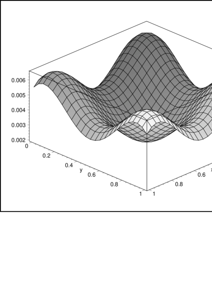
Figure 1: Renormalized local energy density of the minimally coupled scalar field in the interior of the square waveguide.

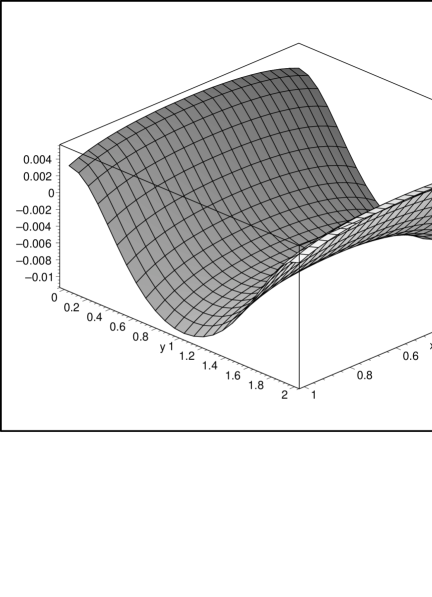
Figure 3: Renormalized local energy density of the minimally coupled scalar field for the $b=2a$ waveguide.

Dowker and Kennedy [14] have evaluated the total energy of the conformally coupled scalar field in the interior of the waveguide for two special configurations. For the square $a=b$, they showed that it assumes a positive value. When $b=2a$ the energy decreases, assuming a negative value. Figures (1) and (2) show the form of $\left\langle T_{00}(\vec{x})\right\rangle_{F}$ and $\left\langle\Theta_{00}(\vec{x})\right\rangle_{F}$ for the square waveguide, assuming $a=b=1$. They present a minimal value in the middle of the waveguide and assume only positive values, which produces a positive value. From the integral of this density one should subtract the constant $C(1,1)$ in order to obtain the total Casimir energy per unit area of the square waveguide. As the value of $b$ increases (for $a=1$), these local quantities acquire negative values in some space points, making the total energy decrease. Figures (3) and (4) show the local energy density in the case $b=2a$. In this case the contribution of the negative part of the local energy dominates and since one still has to subtract $C(1,2)$ from the integral of this energy density, one obtains a negative total energy per unit area.

4 Local forces

In this section we will calculate the local Casimir force density that acts on the walls of the waveguide. To do this we will use the relation between the local force density and the discontinuity of the stress tensor across the walls. Although we don’t know the modes outside the waveguide (because the external mode problem for the waveguide is unsolved), we can introduce an external structure where the modes of the field are known [8], in such a way that the interior region is the interior of the waveguide. One way to do this is connecting two parallel infinite Dirichlet planes by two strips. In this configuration, we know the modes in all regions and the stress tensor can be calculated anywhere. Let us position two parallel infinite Dirichlet planes at $x_{1}=0$ and $x_{1}=a$ and connect these planes by two strips, positioned at $x_{2}=0$ and $x_{2}=b$. The interior region of this configuration is just the waveguide. In the regions $x_{1}>a$ and $x_{1}<0$ there are no contributions from the stress tensor to forces that act in the two infinite planes ($\left<T_{11}(\vec{x})\right>_{ext}=0$). In the regions $0<x_{1}<a,\ x_{2}>b$ and $0<x_{1}<a,\ x_{2}<0,$ the components of the stress tensor have a nonzero contribution to the forces that act on the strips. In these regions the stress tensor has already been calculated in [8]. For completeness, we present the relevant component here, i.e., $\left<T_{22}\left(\vec{x}\right)\right>_{ext}$:

$$\left<T_{22}\left(\vec{x}\right)\right>_{ext} = \frac{1}{32\pi^{2}}\sum_{n=-\infty}^{\infty}\left((na)^{-4}+2(na+x_{1})^{-4}\right.$$ (89)

$$\hskip 28.45274pt\left.-3\left[(na+x_{1})^{2}+x_{2}^{2}\right]^{-2}+4x_{2}^{-4}\left[1+\left(\frac{na+x_{1}}{x_{2}}\right)^{2}\right]^{3}\right).$$

The equation above will serve to compute the local Casimir force that acts on the strip at $x_{2}=0$ (a similar one exists for the strip at $x_{2}=b$). We note that the edge divergences above at $(x_{1},x_{2})=(0,0),(a,0)$ will not be canceled, when we come to calculate the local force, by those of the interior of the waveguide that appear in eq.(62). Nevertheless neither the equation above nor eq.(62) present wall divergences as $x_{2}\rightarrow 0$. Thus the local Casimir force at the strip at $x_{2}=0$ diverges only at the edges, but not on the strip.

We note also that the components $\left<T_{21}\left(\vec{x}\right)\right>_{ext}$ and $\left<T_{12}\left(\vec{x}\right)\right>_{ext}$ vanish on the walls. To obtain the local forces, we use the local force density that acts on the point $\vec{x}$ and is given by $f_{i}\left(\vec{x}\right)=-\partial_{j}T_{ij}\left(\vec{x}\right).$ Thus the local force per unit area on the boundary plane at $x_{1}=0$ is:

$$\frac{F(x_{2})}{A} = \lim_{\varepsilon\rightarrow 0}\left[\left<T_{11}\left(x_{1}=-\varepsilon\right)\right>-\left<T_{11}\left(x_{1}=\varepsilon\right)\right>\right]$$ (90)

$$= \frac{1}{32\pi^{2}}\sum_{n_{1},n_{2}=-\infty}^{\infty}\left(\right.4\left[(n_{1}a)^{2}+(n_{2}b)^{2}\right]^{-3}\left[n_{1}a\right]^{2}+$$

$$\hskip 28.45274pt-4\left[(n_{1}a)^{2}+\left(n_{2}b+x_{2}\right)^{2}\right]^{-3}\left[n_{1}a\right]^{2}+$$

$$\hskip 28.45274pt-\left[(n_{1}a)^{2}+(n_{2}b)^{2}\right]^{-2}+\left[(n_{1}a)^{2}+\left(n_{2}b+x_{2}\right)^{2}\right]^{-2}\left.\right),$$

in the positive $x_{1}-$direction, and an equal but opposite force acts in the plate at $x_{1}=a$. (We have to exclude the term $(n_{1}=n_{2}=0)$ in the third and fourth sums and the term $(n_{1}=0,n_{2}=-1)$ in the fourth sum. The last two exclusions accounts for the renormalization of the edge divergences.)

The force on the wall parallel to the plane at $x_{2}=0$ is given by

$$\frac{F(x_{1})}{A} = \lim_{\varepsilon\rightarrow 0}\left[\left\langle T_{22}\left(x_{2}=-\varepsilon\right)\right\rangle-\left\langle T_{22}\left(x_{2}=\varepsilon\right)\right\rangle\right]$$ (91)

$$= \frac{1}{32\pi^{2}}\sum_{n=-\infty}^{\infty}\{\left(an\right)^{-4}-\left(an+x_{1}\right)^{-4}\}+$$

$$-\frac{1}{32\pi^{2}}\sum_{n_{1},n_{2}=-\infty}^{\infty}\left(\right.-4\left[(n_{1}a)^{2}+(n_{2}b)^{2}\right]^{-3}\left[n_{2}b\right]^{2}+$$

$$\hskip 28.45274pt+4\left[\left(n_{1}a+x_{1}\right)^{2}+(n_{2}b)^{2}\right]^{-3}\left[n_{2}b\right]^{2}+$$

$$\hskip 28.45274pt+\left[(n_{1}a)^{2}+(n_{2}b)^{2}\right]^{-2}-\left[\left(n_{1}a+x_{1}\right)^{2}+\left(n_{2}b\right)^{2}\right]^{-2}\left.\right)$$

$$= \frac{1}{32\pi^{2}}\sum_{n_{1},n_{2}=-\infty}^{\infty}\left(4\left[(n_{1}a)^{2}+(n_{2}b)^{2}\right]^{-3}\left[n_{2}b\right]^{2}-4\left[\left(n_{1}a+x_{1}\right)^{2}+(n_{2}b)^{2}\right]^{-3}\left[n_{2}b\right]^{2}\right)+$$

$$+\frac{1}{16\pi^{2}}\sum_{n_{1}=-\infty}^{\infty}\sum_{n_{2}=1}^{\infty}\left(-\left[(n_{1}a)^{2}+(n_{2}b)^{2}\right]^{-2}+\left[\left(n_{1}a+x_{1}\right)^{2}+\left(n_{2}b\right)^{2}\right]^{-2}\right).$$

An equal but opposite force acts on the wall at $x_{2}=b.$ (The edge divergences of eq.(89) do not cancel those of eq.(62), as we have stressed; nevertheless these were discarded when calculating the local force above, and thus they do not appear.)

Let us analyse how the local forces calculated above depend on the relative sizes of the waveguide. Figure (5) shows the dependence on $x_{2}$ of the finite part of the local force that acts on the wall parallel to the plane $x_{1}=0$. It assumes only negative values and thus it is a repulsive force, in agreement with global calculations. The modulus of the force has a minimum in the middle of the wall and two maxima near the edges. Figure (6) shows the depence on $x_{1}$ of the force on the wall parallel to the plane $x_{2}=0$. It is an attractive force but with only one maximum in the middle of the wall. Although the global computation for the square waveguide gives a repulsive force in all walls, our attractive result is due to the external structure.

Figures (7) and (8) show the forces that act on the walls at $x_{1}=0$ and $x_{2}=0$ when $b=2a$. The local force at $x_{1}=0$ assumes only positive values which makes it an attractive force, as we expect by approaching the parallel plate configuration, but still highly non-uniform. The force at $x_{2}=0$ assumes only positive values and it is very small in comparison with the previous force. As $b$ grows, this force vanishes and the force at $x_{1}=0$ behaves like the uniform Casimir force in the parallel plate configuration as figure (9) shows.

5 Conclusions

In this paper we obtained the canonical and the improved stress-energy tensors of a massless scalar field in the interior of an infinitely long waveguide. The result found is strongly position dependent as expected. Although the global Casimir effect is related to experiments where we measure the force between macroscopic surfaces, the local properties of the vacuum field fluctuations can in principle be observed by measuring the energy level shift of an atom interacting with the electromagnetic field. In the case of the local problem, surface and edge divergences appear related with the uncertainty principle. In order to compute the local forces we introduced an external configuration for which it is possible to solve the eigenmode problem. We have shown that the particular external configuration that we chose was not able to eliminate the wall and edge divergences of the interior of the waveguide. In order to eliminate them two possible ways are to take into account the real properties of the material, i.e., imperfect conductivity at high frequencies, or else make a quantum mechanical treatment of the boundary conditions, as was done by Ford and Svaiter [19]. An alternative method of calculation (using a modified version of the Green’s function method) to find the renormalized stress-energy tensor associated with the scalar field defined in the interior of an infinitely long waveguide is under investigation by the authors.

We have also shown that the integral inside the cavity of the local result gives the known values for the global calculations, although the integral of the finite part of $\left<T_{00}(\vec{x})\right>$ gives the total Casimir energy plus a constant dependent on the waveguide sizes $C(a,b)$.

6 Acknowlegement

This paper is supported by the Conselho Nacional de Desenvolvimento Cientifico e Tecnológico do Brasil (CNPq), and by Fundação de Amparo à Pesquisa do Estado de Minas Gerais (FAPEMIG).

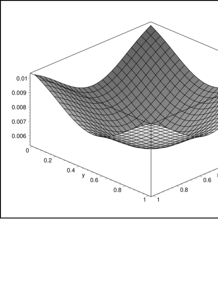
Figure 2: Renormalized local energy density of the conformally coupled scalar field in the interior of the square waveguide.

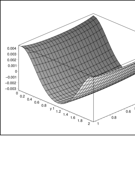
Figure 4: Renormalized local energy density of the conformally coupled scalar field for the $b=2a$ waveguide.

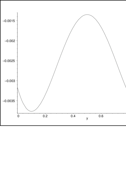
Figure 5: Renormalized local force density that acts on $x_{1}=0$ wall for the square waveguide.

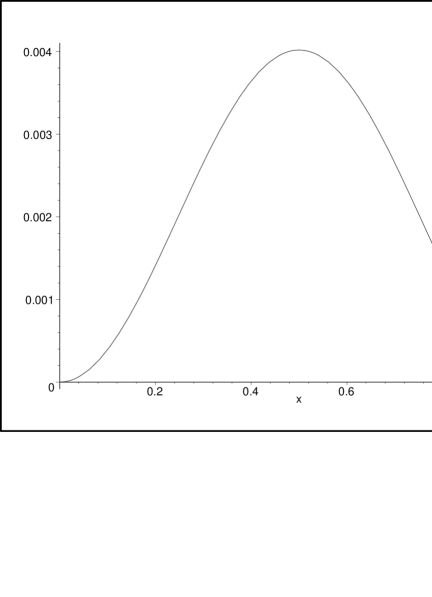
Figure 6: Local force density that acts on $x_{2}=0$ wall for the square waveguide.

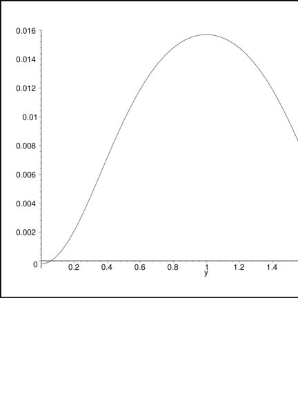
Figure 7: Renormalized local force density that acts on $x_{1}=0$ wall for the $b=2a$ waveguide.

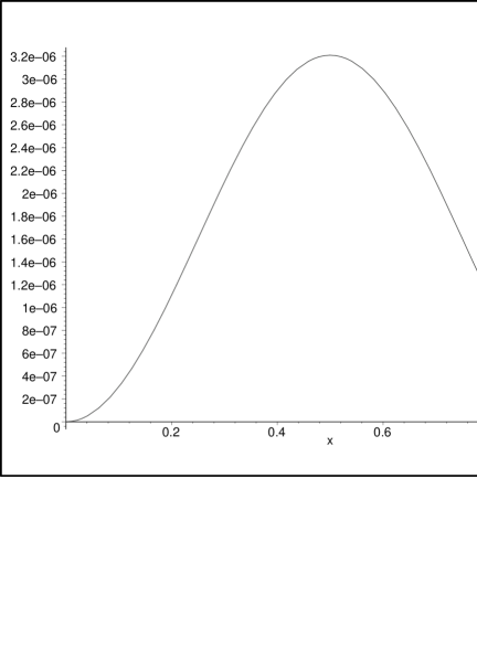
Figure 8: Local force density that acts on $x_{2}=0$ wall for the $b=2a$ waveguide.

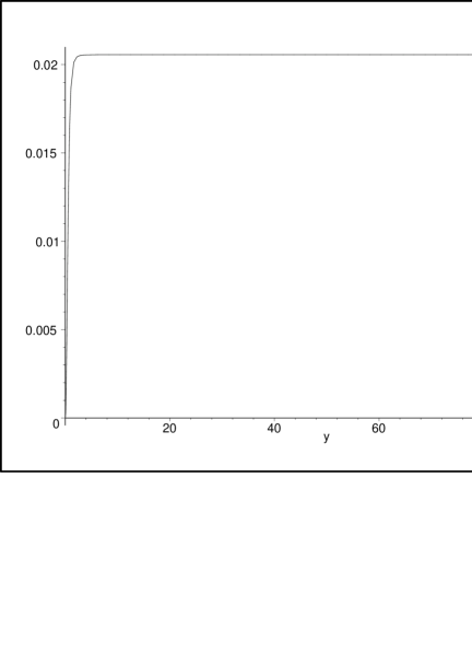
Figure 9: Renormalized uniform force density that acts on $x_{1}=0$ wall when $b>>a$.

References

• [1] C.D. Fosco and N.F. Svaiter, CBPF pre-print NF-052/99, hep-th 9910068; Proceedings of Second International School of Field Theory and Gravitation, Vitoria, Brasil (2000).
• [2] B.S. DeWitt, Phys. Rep. 19, 259 (1975).
• [3] D. Deutsch and P. Candelas, Phys. Rev. D20, 3063 (1979).
• [4] L.H. Brown and G.J. Maclay, Phys. Rev. 184, 1272 (1976).
• [5] G.J. Maclay, Phys.Rev.A61, 052110 (2000).
• [6] B.S. Kay, Phys. Rev. D20, 3052 (1979).
• [7] A.A. Actor, Ann. Phys. 230, 303 (1994); Fortschr. Phys. 43, 141 (1995).
• [8] A.A. Actor and I. Bender, Fortschr. Phys. 44, 281 (1996).
• [9] W. Lukosz, Z. Phys. 258, 99 (1973).
• [10] F. Caruso, N.P. Neto, B.F. Svaiter and N.F. Svaiter, Phys. Rev. D43, 1300 (1991).
• [11] N.F. Svaiter and B.F. Svaiter, J.Math.Phys. 32, 175 (1991); J. Phys. A25, 979 (1992).
• [12] J. Ambjorn and S. Wolfram, Ann. Phys. 147, 1 (1983).
• [13] K.A. Milton and Y. Jack Ng, Phys. Rev. D42, 2875 (1990).
• [14] J.S. Dowker and G. Kennedy, J. Phys. A11, 895 (1978).
• [15] B.F. Svaiter and N.F. Svaiter, J. Math. Phys. 35, 1840 (1994).
• [16] I.S. Gradshteyn and I.M. Ryzhik, in Table of Integrals and Products, edited by A. Jeffrey (Academic, New York, 1980).
• [17] K. Olaussen and F. Ravndal, Nucl. Phys. B192, 237 (1981).
• [18] K. Symanzik, Nucl. Phys. B190, 1 (1980).
• [19] L.H. Ford and N.F. Svaiter, Phys. Rev. D58, 065007-1, (1998).
Refer to caption