Holomorphic potentials for graded D-branes

Abstract:

We discuss gauge-fixing, propagators and effective potentials for topological A-brane composites in Calabi-Yau compactifications. This allows for the construction of a holomorphic potential describing the low-energy dynamics of such systems, which generalizes the superpotentials known from the ungraded case. Upon using results of homotopy algebra, we show that the string field and low energy descriptions of the moduli space agree, and that the deformations of such backgrounds are described by a certain extended version of ‘off-shell Massey products’ associated with flat graded superbundles. As examples, we consider a class of graded D-brane pairs of unit relative grade. Upon computing the holomorphic potential, we study their moduli space of composites. In particular, we give a general proof that such pairs can form acyclic condensates, and, for a particular case, show that another branch of their moduli space describes condensation of a two-form.

1 Introduction

Calabi-Yau compactifications of type II strings in the presence of D-branes form an interesting class of superstring vacua in four dimensions, with rich potential applications for string phenomenology. Such compactifications have recently attracted a great deal of attention [1, 2, 3, 4, 5, 6, 3, 7, 8, 9]. While compactifications in the presence of one brane are at least conceptually well-understood, the situation is rather different for backgrounds containing more general D-brane configurations, whose systematic study has begun only recently. One of the central problems in the subject is the issue of D-brane composites, i.e. bound states of various D-branes resulting upon condensation of spacetime fields associated with boundary condition changing sectors [1, 2, 10, 11]. The basic process of this type (namely tachyon condensation) is known to lead to a wealth of D-brane composites, whose systematic analysis is rather involved.

Perhaps the most powerful approach to this subject has been proposed in [1]. The strategy is to separate the problem into a ‘topological step’ (described by the associated twisted models [12, 13, 14]), which allows one to classify all composites resulting from condensation of space-time fields associated with open string chiral primaries, and a condition [1, 9], whose role is to identify those composites which are stable under decay.

In view of this description, a better understanding of D-brane condensates requires a detailed study of their topological avatars. While the spectrum of topological composites is by now relatively well-established (being described by objects of certain categories naturally associated with the closed string background), rather little is currently known about another basic aspect, namely their moduli space.

The purpose of this paper is to initiate the study of such moduli spaces. The approach we propose will be based on a particularly explicit formulation of D-brane dynamics which describes the formation of such composites within the framework of topological string field theory [15, 16, 17, 19, 20]. This description results from the basic observation of [21, 22] that topological D-branes of a Calabi-Yau compactification are graded objects. The models of [17, 19, 20] are based on a certain extension of the topological field theories of open A/B strings [14], which is devised to take into account the novel data provided by the D-brane grades. This can be formulated as a ‘graded Chern-Simons field theory’, a version of Chern-Simons theory based on a graded superbundle.

A preliminary study of these models was carried out in [16, 17, 19], which gave arguments relating their moduli spaces to certain enhanced triangulated categories naturally associated with the problem. It was also argued in [19] that the moduli space of such theories can be viewed as a certain ‘extended’ version of the moduli space of ungraded D-branes. In this description, ‘nonstandard’ directions in the extended moduli space correspond to condensation processes, and nonstandard moduli points are associated with topological brane composites. Hence one may study such points with usual field-theoretic tools. Moreover, it was showed in [20] that graded Chern-Simons theories are consistent as classical BV systems, and thus form a good starting point for a quantum analysis.

From a mathematical perspective, the moduli spaces discussed in [19, 20] correspond to a deformation problem, whose local description is of Maurer-Cartan type. Since the resulting deformations may be obstructed, a detailed analysis of the moduli space requires a systematic study of obstructions.

In fact, obstructed deformations are also common in ungraded D-brane systems. A method of dealing with obstructions (as they apply to the ungraded case) was proposed in [24], where it was shown that the correct moduli space can be described in terms of a certain potential for the massless modes . This potential, which is extremely natural from a string field-theoretic point of view, coincides with the D-brane superpotentials of [4] (see also [6]). Moreover, the potential is intimately related to certain constructions of modern deformation theory [25, 26, 27, 28] (see also [29]), which were used to establish the main result of [24]. One advantage of this approach is that it allows for a description of the moduli space which does not involve differential equations –and thus is often more effective from a computational point of view. As explained for example in [26, 27], this is intimately connected with standard constructions of Kuranishi theory [30].

Since the definition of the potential given in [24] is purely field-theoretic in nature, one expects that it extends to the graded theories of [19, 20, 17]. In this paper, we show that this is indeed the case. In particular, we shall build a holomorphic potential which is a natural extension of the brane superpotentials of [24] to the case of graded D-branes. Moreover, the arguments of [24] can be adapted to this situation in order to show that the holomorphic potential we construct provides an equivalent description of the moduli space. This allows us to determine the moduli space of topological composites for a particular class of graded D-brane pairs of unit relative grade.

The present paper is organized as follows. In Section 2, we discuss some basic aspects of the theories under study. The models we consider describe arbitrary collections of topological D-branes wrapping a given special Lagrangian cycle of a Calabi-Yau threefold compactification, and provide a description of chiral primary dynamics. After reviewing the origin and structure of such theories, we discuss their gauge symmetries and moduli spaces. We also construct a certain conjugation operator and characterize the associated zero modes in terms of Hodge theory. Section 3 considers the example of D-brane pairs with unit relative grade. Upon using the methods of Section 2, we analyze harmonic modes of such a system. This leads to a completely general discussion of acyclic composites, which extends certain results of [20]. We also give a preliminary analysis of the relevant moduli spaces. In Section 4, we consider the partition function of our models and give a physical definition of a holomorphic potential for virtual deformations (a.k.a. massless, or harmonic modes). Upon using a straightforward extension of the gauge-fixing condition employed in [24], we discuss the tree-level expansion of the potential around a classical solution and the algebraic structure of scattering products. Applying results of modern deformation theory, we show that the moduli space can be described locally as a quotient of the critical set of the potential through the action of certain symmetries. This generalizes the results of [24] to the case of graded D-branes. The results of this section assume consistency of our gauge-fixing procedure. A general proof of this statement, which requires the Batalin-Vilkovisky formalism, turns out to be quite technical and will be given in a companion paper [32]. The main results of that analysis are summarized in Subsection 4.2. Section 5 considers the application of our methods to graded D-brane pairs (of unit relative grade) on a three-torus. For the singly-wrapped case, we compute the holomorphic potential and its symmetry group, and give a local description of the moduli space. We also make a few observation about the multiply-wrapped case. Section 6 presents our conclusions and a few directions for further research. Appendix A contains some technical details, while Appendix B gives an alternate (but equivalent) construction of the tree-level approximation to the holomorphic potential.

2 Structure of the string field theory

Consider a special Lagrangian 3-cycle $L$ of a Calabi-Yau threefold $X$. Throughout this paper, we assume that $L$ is connected. We shall be interested in systems of graded topological D-branes (of different grades) wrapping this cycle. As argued in [19], such systems are described (in the large radius limit) by a string field theory which is a graded form of Chern-Simons field theory. To formulate this, we first review the ‘BPS grade’ of [5, 1, 2, 9] and its relation with a choice of orientation of the cycle [19].

2.1 The BPS grade

Let $\Omega$ be the holomorphic 3-form of $X$, normalized such that $\frac{\omega^{3}}{3!}=\frac{i}{8}\Omega\wedge{\overline{\Omega}}$. In this case, $\Omega$ is determined up to a phase, which we fix for what follows. Recall that a Lagrangian cycle $L$ is special Lagrangian (this description follows from Proposition 2.11 of [18]) if there exists a complex number $\lambda$ of unit modulus such that:

$$Im(\lambda\Omega)|_{L}=0~{}~{}.$$ (2.1)

This condition determines $\lambda$ up to a sign ambiguity ($\lambda\rightarrow-\lambda$), so that only the complex quantity $\lambda^{2}$ is naturally defined by the (unoriented) cycle $L$. Given a choice for $\lambda$, the real 3-form $\lambda\Omega|_{L}$ is nondegenerate and thus induces an orientation ${\cal O}_{\lambda}$ of $L$. When endowed with this orientation, $L$ is a calibrated submanifold of $X$ with respect to the calibration given by $Re(\lambda\Omega)$. In particular, one has:

$$Re(\lambda\Omega)|_{L}=\lambda\Omega|_{L}=vol_{L,{\cal O}_{\lambda}}~{}~{},$$ (2.2)

where $vol_{L,{\cal O}_{\lambda}}$ is the volume form on $L$ induced by the Calabi-Yau metric of $X$ and the orientation ${\cal O}_{\lambda}$. We have $\int_{L,{\cal O}_{L}}\Omega=\frac{\beta}{\lambda}$, where $\beta=vol(L)=|\int_{L}\Omega|>0$ is a positive number. Hence:

$$\lambda^{-1}=\frac{\int_{L,{\cal O}_{\lambda}}\Omega}{|\int_{L}\Omega|}\Leftrightarrow\lambda_{\cal O}^{-1}=\frac{\int_{L,{\cal O}}\Omega}{|\int_{L}\Omega|}~{}~{},$$ (2.3)

which shows how an orientation ${\cal O}$ of $L$ determines $\lambda$.

Following [2, 9], we define the BPS grade of the oriented cycle $(L,{\cal O})$ via:

$$\phi_{L,{\cal O}}=\frac{1}{\pi}{\rm arg}\int_{L,{\cal O}}\Omega=\frac{1}{\pi}{\rm Im}\log\int_{L,{\cal O}}\Omega~{}~{}.$$ (2.4)

Note that $\phi_{L,{\cal O}}$ only depends on the homology class $[L,{\cal O}]$ of the oriented cycle $(L,{\cal O})$ (the pushforward of its fundamental class through the inclusion map). With this definition, we have:

$$\lambda_{\cal O}=e^{-i\pi\phi_{L,{\cal O}}}\Rightarrow\lambda^{2}=e^{-2i\pi\phi_{L,{\cal O}}}~{}~{}.$$ (2.5)

It is clear that $\phi_{L,{\cal O}}$ is determined by $(L,{\cal O})$ only up to a shift by $2$. Moreover:

$$\phi_{L,-{\cal O}}=\phi_{L,{\cal O}}+1~{}~{}(mod~{}2)~{}~{}.$$ (2.6)

Note that there exists a ‘fundamental’ choice of grading, namely $\phi\in[0,1)$. This induces the ‘fundamental orientation’ ${\cal O}_{0}$ for which $Im(\lambda^{-1}_{{\cal O}_{0}})>0$.

It can be argued in various ways that a consistent description of D-brane systems forbids one from restricting $\phi$ to a fundamental domain (of length two). The basic picture is as follows. Following the approach of [34, 15], we are given a closed conformal field theory (parameterized by the complex and Kahler structure of $X$), whose moduli space ${\cal Q}$ can be described as a product between the complex structure moduli space of $X$ and that of its mirror. For any point in this moduli space (i.e. for a fixed closed CFT background), we are interested in the category of all D-branes compatible with this bulk CFT; in the language of [34, 15], this is the category of open-closed extensions of the bulk theory. Invariance of our physical description requires that this category ${\cal C}$ be well-defined at every point in ${\cal Q}$. In general, a given D-brane cannot be deformed to an object which is stable throughout this moduli space; moreover, monodromies around the discriminant loci will act nontrivially on the category ${\cal C}$. The requirement of a well-defined theory implies that the monodromy group be represented through ‘autoequivalences’ (in an appropriate sense) of ${\cal C}$. This condition must hold both at the topological level (i.e. if ${\cal C}$ consists of all topological D-branes compatible with the bulk theory) and at the level of stable BPS branes. Restricting to the topological D-brane category, it is clear that such monodromies will shift the grade of various objects outside of any fundamental domain, which is why one must consider all branches of (2.4). The monodromy action should be viewed as a group of discrete gauge-invariances of the topological D-brane theory.

Using such monodromy actions (for example, monodromy around a large complex structure point of $X$, with the Kahler parameters kept close to large radius), one can generally produce objects of ${\cal C}$ based on the cycle $L$, but whose grades are shifted by $2n$ for any $n\in\hbox{\mybb Z}$; we shall call such objects the ‘shifts’ of $L$. As argued in [15, 16], the full category of topological D-branes must in fact be enlarged to the collection of all topological brane composites, which result by considering all condensation processes of spacetime-fields associated with topological boundary condition changing operators. A monodromy-invariant description requires that we consider condensates between an object and its shifts. In this paper, we are interested in the sector of topological string field theory which describes the formation of such condensates.

Given a special Lagrangian cycle $L$, let us thus consider the collection of all its shifts $L[2n]$ (with $n\in\hbox{\mybb Z}$). Since changing the orientation of $L$ is related (modulo a change in GSO projections) to passing from a brane to its antibrane, and in view of relation (2.6), one must in fact also consider shifts $L[2n+1]$ by odd integers. Hence a complete description of D-branes wrapping $L$ must consider all integral shifts of $L$. For any such brane $L[n]$, one also specifies a background given by a flat connection $A_{n}$ in a complex vector bundle $E_{n}$ over $L$. Since we work with the topological model, there is no need to impose (anti) hermicity conditions on $A_{n}$ (we shall allow the string field action to be complex ). Given this data, it was argued in [19] that the topological string field theory of the D-brane collection $(L[n],A_{n})$ is a ‘graded Chern-Simons model’, which we now explain.

2.2 Ingredients of the topological model

Given a collection of graded branes (of different grades $n$) wrapping $L$, we form the total bundle ${\bf E}=\oplus_{n}{E_{n}}$, endowed with the ℤ-grading induced by $n$. As argued in [19], the presence of D-brane grades which differ by integers shifts the assignment of worldsheet $U(1)$ charge in the various boundary condition changing sectors. The result is that the charge of states of strings stretching from $E_{m}$ to $E_{n}$ is shifted by $n-m$. Since such states localize [14] on differential forms on $L$, valued in $Hom(E_{m},E_{n})$, the worldsheet charge induces a grading $|.|$ on the space of $End({\bf E})$-valued forms:

$$|u|=rku+\Delta(u)~{}~{},$$ (2.7)

where $\Delta(u)=n-m$ if $u\in\Omega^{*}(L,Hom(E_{m},E_{n}))$. In geometric terms, we are interested in sections $u$ of the bundle:

$${\cal V}=\Lambda^{*}(T^{*}L)\otimes End({\bf E})~{}~{},~{}~{}$$ (2.8)

endowed with the grading ${\cal V}=\oplus_{t}{{\cal V}^{t}}$, where:

$${\cal V}^{t}=\oplus_{\tiny\begin{array}[]{c}k,m,n\\ k+n-m=t\end{array}}{\Lambda^{k}(T^{*}L)\otimes Hom(E_{m},E_{n})}~{}~{}.$$ (2.9)

The space ${\cal H}=\Gamma({\cal V})$ of such sections is the total boundary space of [19], and can be interpreted as the collection of all open string states of the system. It is endowed with the grading ${\cal H}^{k}=\Gamma({\cal V}^{k})$.

The second ingredient of [19] is the so-called total boundary product, which is defined through:

$$u\bullet v=(-1)^{\Delta(u)rkv}u\wedge v~{}~{},$$ (2.10)

where the wedge product on the right hand side includes composition of morphisms in $End({\bf E})$. As discussed in [19] that this product is associative (albeit not commutative, in general). It also admits the identity endomorphism $1$ of ${\bf E}$ as a neutral element:

$$1\bullet u=u\bullet 1=u~{}~{}.$$ (2.11)

Moreover, the product is compatible with the grading on ${\cal H}$:

$$|u\bullet v|=|u|+|v|~{}~{}$$ (2.12)

(note that $|1|=0$), and thus endows this space with a structure of graded associative algebra.

The third ingredient arises by noticing that ${\bf E}$ is endowed with a flat structure, the direct sum of flat structures on the bundles $E_{n}$. This can be described by the direct sum connection $A^{(0)}=\oplus_{n}{A_{n}}$. The flat connection $A^{(0)}$ determines a nilpotent differential $d$ on ${\cal H}$, the de Rham differential coupled to the connection induced by $A^{(0)}$ on $End({\bf E})$. This operator acts as a degree one derivation of the boundary product:

$$|du|=|u|+1~{}~{},~{}~{}d(u\bullet v)=(du)\bullet v+(-1)^{|u|}u\bullet(dv)~{}~{}.$$ (2.13)

Endowed with the product $\bullet$ and this differential, ${\cal H}$ becomes a differential graded associative algebra (dGA).

The final ingredient of [19] is a bilinear form on ${\cal H}$ induced by the graded trace on the bundle $End({\bf E})$. The latter is defined through:

$$str(u)=\sum_{n}{(-1)^{n}tr(u_{nn})}~{}~{},~{}~{}{\rm for}~{}~{}u=\oplus_{m,n}{u_{mn}}~{}~{},$$ (2.14)

with $u_{mn}\in\Omega^{*}(L,Hom(E_{m},E_{n}))$. This associates a form with complex coefficients to every $End({\bf E})$-valued form on $L$. The bilinear form:

$$\langle u,v\rangle:=\int_{L}{str(u\bullet v)}~{}~{}$$ (2.15)

is non-degenerate and has the properties:

$$\langle u,v\rangle=(-1)^{|u||v|}\langle v,u\rangle~{}~{}$$

$$\langle du,v\rangle+(-1)^{|u|}\langle u,dv\rangle=0~{}~{}$$ (2.16)

$$\langle u\bullet v,w\rangle=\langle u,v\bullet w\rangle~{}~{}.$$

In words, it is a graded-symmetric, invariant bilinear form on the differential graded algebra $({\cal H},d,\bullet)$. In (2.15) and in all other integrals over $L$, we assume that the special Lagrangian cycle has been endowed with its ‘fundamental’ orientation ${|calO}_{0}$ (see [19] and Subsection 2.1).

2.3 The action

The string field theory of [19, 20] is described by the action:

$$S(\phi)=Re\int_{L}{str\left[\frac{1}{2}\phi\bullet d\phi+\frac{1}{3}\phi\bullet\phi\bullet\phi\right]}=\frac{1}{2}\langle\phi,d\phi\rangle+\frac{1}{3}\langle\phi,\phi\bullet\phi\rangle~{}~{}~{}~{},$$ (2.17)

which is defined on the degree one component

$${\cal H}^{1}=\{\phi\in{\cal H}||\phi|=1\}=\Gamma(\oplus_{k+n-m=1}{\Lambda^{k}(T^{*}L)\otimes Hom(E_{m},E_{n})})$$ (2.18)

of the total boundary space. This action defines a ‘graded Chern-Simons field theory’, which is related to, but not identical with, the super-Chern-Simons field theory considered in [33, 23]. The physics described by (2.17) is considerably more complicated than that of usual or super-Chern-Simons theories.

2.4 Gauge symmetries

The theory (2.17) is invariant with respect to a gauge group which can be described as follows. Since the boundary product is compatible with the degree $|.|$, it follows that the subspace ${\cal H}^{0}=\Gamma(\oplus_{k+n-m=0}{\Lambda^{k}(T^{*}L)\otimes Hom(E_{m},E_{n})})$ of charge zero elements of ${\cal H}$ forms a subalgebra of the total boundary algebra $({\cal H},\bullet)$. Since $|1|=0$, this subalgebra has a unit. It follows that the set:

$${\cal G}=\{g\in{\cal H}^{0}|{\rm~{}exists~{}}~{}g^{-1}\in{\cal H}^{0}~{}{\rm~{}such~{}that~{}}~{}g\bullet g^{-1}=g^{-1}\bullet g=1\}~{}~{}$$ (2.19)

of invertible elements of $({\cal H}^{0},\bullet)$ forms a group with respect to the boundary multiplication. Its adjoint action:

$$u\rightarrow Ad_{g}(u):=g\bullet u\bullet g^{-1}~{}~{},~{}~{}{\rm~{}for~{}}~{}~{}u\in{\cal H}~{}~{},~{}~{}g\in{\cal G}$$ (2.20)

on the total boundary space preserves the worldsheet degree $|.|$, and in particular induces an action on the subspace ${\cal H}^{1}$ of degree one states.

If $g$ is close to the identity, then one can use the exponential parameterization:

$$g=e^{\alpha}_{\bullet}:=\sum_{k\geq 0}{\frac{1}{k!}\alpha^{\bullet k}}~{}~{},$$ (2.21)

where $\alpha^{\bullet k}$ stands for $k$-th iteration of the $\bullet$-product of $\alpha$ with itself (and we define $\alpha^{\bullet 0}:=1$). In particular, the Lie algebra of ${\cal G}$ can be described as follows. For any two elements $u,v$ of ${\cal H}$, we define their graded commutator by:

$$[u,v]_{\bullet}:=u\bullet v-(-1)^{|u||v|}v\bullet u~{}~{}.$$ (2.22)

This bracket is graded antisymmetric:

$$[u,v]_{\bullet}=-(-1)^{|u||v|}[v,u]_{\bullet}$$ (2.23)

and satisfies the graded Jacobi identity:

$$[[u,v]_{\bullet},w]_{\bullet}+(-1)^{|u|(|v|+|w|)}[[v,w]_{\bullet},u]_{\bullet}+(-1)^{|w|(|u|+|v|)}[[w,u]_{\bullet},v]_{\bullet}=0~{}~{},$$ (2.24)

as well as the relation:

$$d[u,v]_{\bullet}=[du,v]_{\bullet}+(-1)^{|u|}[u,dv]_{\bullet}~{}~{},$$ (2.25)

thereby making ${\cal H}$ into a differential graded Lie algebra (dGLA). The subspace ${\cal H}^{0}$ of degree zero elements is closed under the bracket, and forms a usual Lie algebra with respect to the induced operation, which on degree zero elements coincides with the standard commutator:

$$[\alpha,\beta]_{\bullet}=\alpha\bullet\beta-\beta\bullet\alpha~{}~{}{\rm~{}~{}for~{}~{}}~{}~{}\alpha,\beta\in{\cal H}^{0}~{}~{}.$$ (2.26)

It is clear that $({\cal H}^{0},[.,]_{\bullet})$ coincides with the Lie algebra of the gauge group ${\cal G}$. Differentiating (2.20) shows that this algebra acts on ${\cal H}$ through its adjoint representation:

$$u\rightarrow ad_{\alpha}(u):=[\alpha,u]_{\bullet}~{}~{}.$$ (2.27)

By analogy with usual Chern-Simons theory, we consider the gauge transformations:

$$\phi\rightarrow\phi^{g}=g\bullet\phi\bullet g^{-1}+g\bullet dg^{-1}~{}~{}.$$ (2.28)

Upon using the derivation property of $d$, the identity $g\bullet g^{-1}=g^{-1}\bullet g=1$ implies:

$$dg^{-1}=-g^{-1}\bullet(dg)\bullet g^{-1}~{}~{}.$$ (2.29)

Combining this identity with the invariance properties of the bilinear form, one can check that the action (2.17) transforms as follows under (2.28):

$$S(\phi)\rightarrow S(\phi^{g})=S(\phi)+\Delta(g)~{}~{},$$ (2.30)

where:

$$\Delta(g)=\frac{1}{6}\int_{L}{str(g^{-1}\bullet dg\bullet g^{-1}\bullet dg\bullet g^{-1}\bullet dg)}~{}~{}.$$ (2.31)

For infinitesimal $\alpha$, the gauge transformations (2.28) become:

$$\phi\rightarrow\phi+\delta_{\alpha}\phi~{}~{},$$ (2.32)

with $\delta_{\alpha}\phi=-d\alpha-[\phi,\alpha]_{\bullet}$, and one can directly check the relation:

$$\delta_{\alpha}\delta_{\beta}\phi-\delta_{\beta}\delta_{\alpha}\phi=\delta_{[\alpha,\beta]_{\bullet}}\phi~{}~{},$$ (2.33)

i.e. the gauge algebra closes off shell. For an infinitesimal transformation (2.32), one has $g^{-1}\bullet dg=d\alpha+O(\alpha^{2})$ and thus the quantity $\Delta(g)$ vanishes to third order in $\alpha$:

$$\Delta(g)=\frac{1}{6}\int_{L}{str(d\alpha\bullet d\alpha\bullet d\alpha)}+O(\alpha^{4})=\frac{1}{6}\int_{L}{dstr(\alpha\bullet d\alpha\bullet d\alpha)}+O(\alpha^{4})=O(\alpha^{4})~{}~{}.$$ (2.34)

This implies:

$$\frac{d}{dt}S(\phi^{e^{t\alpha}_{\bullet}})=0\Rightarrow S(\phi^{e^{t\alpha}_{\bullet}})=S(\phi)~{}~{}{\rm~{}for~{}}~{}~{}\alpha\in{\cal H}^{0}~{}~{}.$$ (2.35)

Taking $t=1$ shows that the action 2.17 is invariant under small gauge transformations, which we define as those gauge transformations which can be written in the exponential form (2.21).

We finally note that the adjoint action (2.28) of a ‘small’ element $g$ can be written as:

$$Ad_{e^{\alpha}_{\bullet}}=e^{ad_{\alpha}}~{}~{},$$ (2.36)

where the right hand side is the formal exponential of $ad_{\alpha}$ viewed as a linear operator in the vector space ${\cal H}$. Moreover, the gauge group action (2.28) takes the form:

$$\phi\rightarrow\phi^{e^{\alpha}_{\bullet}}=e^{ad_{\alpha}}\phi-\frac{e^{ad_{\alpha}}-1}{ad_{\alpha}}d\alpha~{}~{},$$ (2.37)

where the fraction in the last term is formally defined by its power series expansion (better, by functional calculus). This recovers the formulation used in [24].

The ungraded case

Since our description of the gauge group may seem unfamiliar, let us consider what it becomes in the ungraded case. This corresponds to ${\bf E}=E_{0}$, i.e. a single ungraded D-brane wrapping $L$. In this situation, (2.17) reduces to the usual Chern-Simons theory coupled to the bundle $E_{0}$ (and expanded around the background flat connection $A_{0}$). The degree zero component of the total boundary algebra is ${\cal H}^{0}=\Gamma(End(E_{0}))$, the space of endomorphisms of the bundle $E_{0}$; this is endowed with the multiplication given by usual fiberwise composition of morphisms:

$$\alpha\bullet\beta=\alpha\circ\beta~{}~{}.$$ (2.38)

The units of this algebra form the standard gauge group ${\cal G}=\Gamma(Aut(E_{0}))$ of automorphisms of $E_{0}$. Our presentation of ${\cal G}$ in the graded case is the generalization of this description.

2.5 The classical moduli space and its interpretation

The critical points of (2.17) are solutions to the equation:

$$\frac{\delta S}{\delta\phi}=0\Longleftrightarrow d\phi+\frac{1}{2}[\phi,\phi]_{\bullet}=0~{}~{},$$ (2.39)

with $\phi$ an element of ${\cal H}^{1}$ (note that $\frac{1}{2}[\phi,\phi]_{\bullet}=\phi\bullet\phi$ for a degree one element $\phi$). The equation of motion (2.39) is invariant under the gauge group action (2.28) (with $g$ an arbitrary gauge transformation, small or large). The moduli space ${\cal M}$ results upon dividing the space of solutions through this gauge group action. The Maurer-Cartan condition (2.39) describes deformations of the reference connection $A^{(0)}$ into a ‘flat superconnection $A$ of total degree one’ (in the sense of [35]). Hence ${\cal M}$ is the moduli space of such superconnections, defined on the graded bundle ${\bf E}$. The original background $A^{(0)}$ corresponds to a ‘diagonal’ superconnection, constructed as a direct sum of flat connections on the bundles $E_{n}$.

The adjoint and gauge-group actions (2.20,2.28) preserve the degree $|.|$. The total grading of the bundle ${\cal V}$ is a gauge-invariant concept, and the collection ${\cal S}$ of flat degree one superconnections is well-defined. The gauge-group action (2.28) preserves ${\cal S}$, and the moduli space ${\cal M}$ can be defined geometrically as the quotient ${\cal M}={\cal S}/{\cal G}$. A reference point is only necessary when writing the Maurer-Cartan equation (2.39). In physical terms, a reference superconnection appears because we use a background-dependent formulation of the string field theory.

In general, ${\cal M}$ is a rather complicated object, which depends on the topology of $L$ and on the structure of the graded superbundle ${\bf E}$. It is clear that this moduli space can have singularities or fail to be compact, and that a global study requires some careful analysis in the manner familiar from the usual theory of flat connections.

Following [15, 16] and [19], we recall the D-brane interpretation of ${\cal M}$. As argued in those papers, an off-diagonal background corresponds to condensation of the spacetime fields associated with the combination of boundary condition changing operators described by the string field $\phi$. This process leads to the formation of D-brane composites, thus altering the brane interpretation of the background. The main observation is that an off-diagonal background violates the original decomposition of the total boundary space into the sectors $\Gamma(\Lambda^{*}(T^{*}L)\otimes Hom(E_{m},E_{n}))$, and thus alters the D-brane content of the theory. When expanded around the new background, the string field action has the same form (2.17) (up to addition of an irrelevant constant), but with a shifted differential:

$$d\rightarrow d_{\phi}~{}~{},~{}~{}d_{\phi}u=du+[\phi,u]_{\bullet}~{}~{}.$$ (2.40)

As explained in [15, 16], the new D-brane content can be identified by studying certain decomposition properties of the shifted differential, together with the boundary product and bilinear form. This can be discussed systematically in the language of category theory [15, 16].

2.6 Virtual dimensions and obstructions

The linearization of (2.39) and (2.28) is specified by:

$$d\phi=0~{}~{},~{}~{}\phi\equiv\phi-d\alpha~{}~{}.$$ (2.41)

Thus first order deformations are in one to one correspondence with elements of the cohomology group $H_{d}^{1}({\cal H}):={\rm ker}(d:{\cal H}^{1}\rightarrow{\cal H}^{2})/{\rm im}(d:{\cal H}^{0}\rightarrow{\cal H}^{1})$. This gives the virtual dimension:

$$vdim_{A}{\cal M}:=h_{1}~{}~{},$$ (2.42)

where $h_{k}$ denotes the dimension of $H^{k}_{d_{A}}({\cal H})$. The approximation (2.41) need of course not suffice, and typically some infinitesimal deformations will be obstructed. Such obstructions lift some directions in $H^{1}_{d}({\cal H})$, leading to a moduli space of dimension smaller than (2.42).

As in [24], our approach to obstructions will be to construct a function $W$ (the holomorphic potential of Section 4), which is defined on the space $H^{1}_{d_{A}}({\cal H})$ of virtual deformations (the ‘virtual tangent space’ to ${\cal M}$ at $A$) and whose critical set gives a local description of the true moduli space after dividing out through some effective symmetries. From this perspective, the potential $W$ is a tool for dealing with obstructions in a systematic manner.

2.7 Harmonic analysis of linearized zero modes

It is convenient to describe the space of virtual deformations through harmonic analysis. In this subsection, we develop the ingredients of such a description, which will be useful in later sections.

2.7.1 The Hermitian scalar product and conjugation operator

Let us pick a Riemannian metric $g$ on the three-manifold $L$ and Hermitian metrics on each of the bundles $E_{n}$, which induce a Hermitian metric on the direct sum ${\bf E}=\oplus_{n}E_{n}$. These metrics (which are arbitrarily chosen) will be kept fixed for what follows (the physics will be independent of all choices).

We first consider the Hermitian conjugation operator $\dagger$ on sections of the bundle $End({\bf E})$. This is involutive and antilinear, and inverts the grading $\Delta$:

$$(f^{\dagger})^{\dagger}=f~{}~{},~{}~{}(\lambda f)^{\dagger}={\overline{\lambda}}f^{\dagger}~{}~{},~{}~{}\Delta(f^{\dagger})=-\Delta(f)~{}~{},$$ (2.43)

for $f\in\Gamma(End({\bf E}))$ and $\lambda$ a complex-valued function on $L$. We also note the properties:

$$str(f^{\dagger})=\overline{str(f)}~{}~{}{\rm~{}and~{}}~{}~{}(f\circ g)^{\dagger}=g^{\dagger}\circ f^{\dagger}~{}~{}.$$ (2.44)

On the space $\Omega^{*}(L)$ of complex-valued forms, we have the complex linear Hodge operator $*$, which is involutive and satisfies:

$$rk(*\omega)=3-rk\omega~{}~{},$$ (2.45)

with $\omega\in\Omega^{*}(L)$. If $(.,.)$ is the metric induced on $\Omega^{*}(L)$ by the Riemannian metric on $L$, then $*$ has the defining property:

$$(*\omega)\wedge\eta=(\omega,\eta)vol_{g}~{}~{},$$ (2.46)

where $vol_{g}$ is the volume form on $L$ induced by $g$. Since $(\omega,\eta)=(\eta,\omega)$, this implies the identity:

$$(*\omega)\wedge\eta=(*\eta)\wedge\omega~{}~{}.$$ (2.47)

Viewing ${\bf E}$ as a usual vector bundle (by forgetting the grading), we have a Hermitian scalar product:

$$h(u,v)=\int_{L}{tr(*u^{\dagger}\wedge v)}~{}~{},~{}~{}u,v\in{\cal H}~{}~{},$$ (2.48)

which takes the following form on decomposable elements $u=\omega\otimes f$ and $v=\eta\otimes g$:

$$h(u,v)=\int_{L}{tr(f^{\dagger}\circ g)(*{\overline{\omega}}\wedge\eta)}~{}~{}.$$ (2.49)

Following [24], we look for an antilinear operator $c$ on ${\cal H}$ with the property:

$$h(u,v)=\langle cu,v\rangle=\int_{L}{str[(cu)\bullet v]}~{}~{}.$$ (2.50)

Since the bilinear form is non-degenerate, this condition determines $c$ uniquely. Upon considering decomposable elements, it is not hard to check that:

$$c(\omega\otimes f)=(-1)^{n+\Delta(f)(1+rk\omega)}(*{\overline{\omega}})\otimes f^{\dagger}~{}~{},~{}~{}{\rm~{}for~{}}~{}~{}\omega\in\Omega^{*}(L)~{}~{}{\rm~{}and~{}}~{}~{}f\in Hom(E_{m},E_{n})~{}~{}.$$ (2.51)

Note the sign factor $(-1)^{n}$ (which depends on the grade of the image of $f$). This is necessary in order to convert the trace in the definition of $h$ to the graded trace appearing in relation (2.50). The operator $c$ satisfies:

$$|cu|=3-|u|~{}~{}.$$ (2.52)

It is also easy to see that $c$ is involutive (i.e. $c^{2}=id$). The Hermitian metric and conjugation operator satisfy all requirements of the abstract framework discussed in [24].

2.7.2 The deformed Laplacian and harmonic modes

For a linear operator $B$ on ${\cal H}$, we let $B^{\dagger}$ denote its Hermitian conjugate with respect to $h$. As shown in [24], the properties of $c$ imply:

$$d^{\dagger}u=(-1)^{|u|}cdcu~{}~{}{\rm~{}and~{}}~{}~{}\langle d^{\dagger}u,v\rangle=(-1)^{|u|}\langle u,d^{\dagger}v\rangle~{}~{}.$$ (2.53)

We also note that $|d^{\dagger}u|=|u|-1$. Let us consider the ‘deformed Laplacian’:

$$\Delta:=d^{\dagger}d+dd^{\dagger}~{}~{},$$ (2.54)

which is a Hermitian, degree zero, elliptic differential operator of order two on ${\cal H}=\Gamma({\cal V})$:

$$|\Delta u|=|u|~{}~{},~{}~{}\Delta^{\dagger}=\Delta~{}~{}.$$ (2.55)

Observation

Given an element $\Phi\in{\cal H}$, such that $|\Phi|$ is odd, consider the operator:

$$A_{\Phi}u:=[\Phi,u]_{\bullet}~{}~{}.$$ (2.56)

It is clear that $A_{\Phi}$ acts as an odd graded derivation of the total boundary product $\bullet$. It is also easy to check (upon using invariance of the bilinear form) that $A_{\Phi}$ acts as derivation of $\langle.,.\rangle$:

$$\langle A_{\Phi}u,v\rangle+(-1)^{|u|}\langle u,A_{\Phi}v\rangle=0~{}~{}.$$ (2.57)

Upon combining this with the definition of $h$ and the property $c^{2}=id$, one obtains that the Hermitian conjugate of $A$ with respect to $h$ has the form:

$$A_{\Phi}^{\dagger}u=(-1)^{|u|}cA_{\Phi}cu~{}~{}.$$ (2.58)

In particular, if $\phi\in{\cal H}^{1}$ is a shift of the background satisfying the equations of motion $d\phi+\phi\bullet\phi=0$, then the shifted differential $d_{\phi}=d+[\phi,\cdot]_{\bullet}=d+A_{\phi}$ is again a degree one derivation of the boundary algebra $({\cal H},\bullet)$, whose Hermitian conjugate has the form:

$$d_{\phi}^{\dagger}u=d^{\dagger}u+A^{\dagger}_{\phi}u=d^{\dagger}u+(-1)^{|u|}c[\phi,cu]=(-1)^{|u|}cd_{\phi}cu~{}~{}.$$ (2.59)

This shows invariance of our formalism with respect to shifts of the string vacuum. In particular, all statements of this section apply to backgrounds $A$ which need not be diagonal.

2.7.3 Hodge decomposition, invertibility properties and dualities on cohomology

As in [24], we consider the Hodge decomposition ${\cal H}=Imd\oplus Imd^{\dagger}\oplus K$, where:

$$K=kerd\cap kerd^{\dagger}=ker\Delta~{}~{} ~{}~{}{\cal H}=K\oplus imd\oplus imd^{\dagger}~{}~{},$$ , (2.60)

$$kerd=K\oplus imd~{}~{}~{}~{}~{}~{}~{}~{}~{}~{}~{}~{}~{}~{} ~{}~{}kerd^{\dagger}=K\oplus imd^{\dagger},$$ , (2.61)

and the propagator $U=\frac{1}{d}\pi_{d}=d^{\dagger}\frac{1}{H}(\pi_{d}+\pi_{d^{\dagger}})=d^{\dagger}\frac{1}{H}\pi_{d}=\frac{1}{H}d^{\dagger}$ (with $H=d^{\dagger}d+dd^{\dagger}$) associated to the gauge $d^{\dagger}\phi=0$, where $\pi_{d}$ and $\pi_{d^{\dagger}}$ are the orthogonal projectors on $imd$ and $imd^{\dagger}$. Physical states of our string field theory correspond to elements of $K^{1}$ (the subspace of degree one states lying in $K$):

$$H^{1}_{d}({\cal H})\approx K^{1}~{}~{}.$$ (2.62)

This isomorphism depends on the choice of metrics on $L$ and ${\bf E}$.

The restriction of $d$ to the orthogonal complement of its kernel maps $(kerd)^{\perp}=imd^{\dagger}$ onto $imd$. This gives a bijection $d:imd^{\dagger}\stackrel{{\scriptstyle\approx}}{{\rightarrow}}imd$. Since $c$ maps $imd$ into $imd^{\dagger}$ and viceversa, it follows that $cd$ and $dc$ give automorphisms of the subspaces $imd^{\dagger}$ and $imd$, respectively. We also note that $c$ preserves the subspace $K$, and intertwines its components according to:

$$c(K^{j})=K^{3-j}~{}~{}.$$ (2.63)

In particular, $c$ induces an isomorphism between $H^{j}_{d}({\cal H})$ and $H^{3-j}_{d}({\cal H})$, which we will loosely call ‘Poincare duality’ (even though it is an isomorphism between two cohomology groups, rather than between homology and cohomology). On the other hand, the non-degenerate bilinear form $\langle.,.\rangle$ gives canonical (and metric-independent) isomorphisms:

$$H^{3-j}_{d}({\cal H})\approx H^{j}_{d}({\cal H})^{*}~{}~{}.$$ (2.64)

The isomorphism induced by $c$ results from this upon composing with the identification induced by $h$ between $H^{j}_{d}({\cal H})$ and its dual.

3 Example: Topological D-brane pairs of unit relative grade in a scalar background

Consider a D-brane pair $(a,b)$ such that $\phi_{a}:=0$ and $\phi_{b}=1$. In this case, the underlying graded bundle is ${\bf E}=E_{a}\oplus E_{b}$, where $E_{a}$ and $E_{b}$ are the flat bundles underlying the D-branes. Throughout this section, we assume that the flat connections $A_{a}$ and $A_{b}$ are unitary with respect to some choice of Hermitian metrics on $E_{a}$ and $E_{b}$, which we shall use in order to build the metric $h$ on ${\cal H}$. This assumption will be necessary for to arrive at a particularly simple form of the deformed Laplacian.

The space ${\cal H}^{k}$ of degree $k$ elements in ${\cal H}$ is the space of sections of the bundle ${\cal V}^{k}=\Lambda^{k}(T^{*}L)\otimes End(E_{a})\oplus\Lambda^{k}(T^{*}L)\otimes End(E_{b})\oplus\Lambda^{k-1}(T^{*}L)\otimes Hom(E_{a},E_{b})\oplus\Lambda^{k+1}(T^{*}L)\otimes Hom(E_{b},E_{a})$. Its elements can be arranged as a matrix of bundle-valued forms:

$$u=\left[\begin{array}[]{cc}u_{k}&u_{k+1}\\ u_{k-1}&{\hat{u}}_{k}\end{array}\right]~{}~{},~{}~{}{\rm for}~{}~{}|u|=k~{}~{},$$ (3.65)

where the subscript denotes form rank and the bundle components of $u_{k}=u_{aa},{\hat{u}}_{k}=u_{bb},u_{k+1}=u_{ba}$ and $u_{k-1}=u_{ab}$ are morphisms from $E_{a}$ to $E_{a}$, $E_{b}$ to $E_{b}$, $E_{b}$ to $E_{a}$ and $E_{a}$ to $E_{b}$ respectively. With this convention, the boundary product agrees with matrix multiplication:

$$(u\bullet v)_{\alpha\beta}=u_{\alpha\gamma}\bullet v_{\gamma\beta}~{}~{}$$ (3.66)

for all $\alpha,\beta\in\{a,b\}$.

We are interested in backgrounds of the form:

$$\phi=\left[\begin{array}[]{cc}0&0\\ \phi_{0}&0\end{array}\right]~{}~{},~{}~{}|\phi|=1~{}~{},$$ (3.67)

where $\phi_{0}$ is a zero-form valued in the bundle $Hom(E_{a},E_{b})$. In this case, the equations of motion $d\phi+\phi\bullet\phi=0$ reduce to $d\phi_{0}=0$, which means that $\phi_{0}$ is a covariantly-constant section of $Hom(E_{a},E_{b})$. Such backgrounds were also considered in [20], where we discussed acyclic composite formation under some (rather stringent) topological assumptions. In this section, we generalize that result by removing all such restrictions, and study other aspects of this system.

3.1 The deformed Laplacian

Let us find the Laplacian $\Delta_{\phi}=d_{\phi}d^{\dagger}_{\phi}+d^{\dagger}_{\phi}d_{\phi}$ in the background (3.67). It turns out that this operator has a particularly simple form for our class of backgrounds. To describe this, we define a graded anticommutator through:

$$\{u,v\}_{\bullet}=u\bullet v+(-1)^{|u||v|}v\bullet u~{}~{}{\rm~{}for~{}}u,v\in{\cal H}~{}~{}.$$ (3.68)

This quantity, which differs from the graded commutator $[u,v]_{\bullet}=u\bullet v-(-1)^{|u||v|}v\bullet u$ by the middle sign factor, has the graded symmetry property:

$$\{u,v\}_{\bullet}=(-1)^{|u||v|}\{v,u\}_{\bullet}~{}~{}.$$ (3.69)

It is shown in Appendix A that the deformed Laplacian can be written as :

$$\Delta_{\phi}u=\Delta u+\{[\phi,\phi^{\dagger}]_{\bullet},u\}_{\bullet}~{}~{},$$ (3.70)

where $\phi^{\dagger}=\left[\begin{array}[]{cc}0&\phi_{0}^{\dagger}\\ 0&0\end{array}\right]$ is the Hermitian conjugate of $\phi$. Note that $|\phi^{\dagger}|=-1$ and:

$$[\phi,\phi^{\dagger}]_{\bullet} = \phi\bullet\phi^{\dagger}+\phi^{\dagger}\bullet\phi=\phi\circ\phi^{\dagger}+\phi^{\dagger}\circ\phi=\{\phi,\phi^{\dagger}\}~{}~{},$$ (3.71)

$$\{[\phi,\phi^{\dagger}]_{\bullet},u\}_{\bullet} = [\phi,\phi^{\dagger}]_{\bullet}\bullet u+u\bullet[\phi,\phi^{\dagger}]_{\bullet}=\{\phi,\phi^{\dagger}\}\circ u+u\circ\{\phi,\phi^{\dagger}\}~{}~{},$$

where $\circ$ denotes composition of fiber morphisms and $\{.,.\}$ is the usual anticommutator taken with respect to this composition. Consider the operator $A_{\phi}u:=[\phi,u]_{\bullet}$. Then it is shown in Appendix A that $A_{\phi}^{\dagger}u=\{\phi^{\dagger},u\}_{\bullet}$. It follows that the last term of (3.70) has the form:

$$\{[\phi,\phi^{\dagger}]_{\bullet},u\}_{\bullet}=(A^{\dagger}_{\phi}A_{\phi}+A_{\phi}A_{\phi}^{\dagger})~{}u~{}~{},$$ (3.72)

and thus $\Delta_{\phi}$ is a sum of three non-negative operators:

$$\Delta_{\phi}=\Delta+A^{\dagger}_{\phi}A_{\phi}+A_{\phi}A_{\phi}^{\dagger}~{}~{}.$$ (3.73)

Upon noticing that $[\phi,\phi^{\dagger}]_{\bullet}=\left[\begin{array}[]{cc}\phi_{0}^{\dagger}\circ\phi_{0}&0\\ 0&\phi_{0}\circ\phi_{0}^{\dagger}\end{array}\right]$, we use (3.70) to obtain the component form:

$$\Delta_{\phi}u=\left[\begin{array}[]{cc}\Delta u_{k}+u_{k}\circ\phi_{0}^{\dagger}\circ\phi_{0}+\phi_{0}^{\dagger}\circ\phi_{0}\circ u_{k}&\Delta u_{k+1}+u_{k+1}\circ\phi_{0}\circ\phi_{0}^{\dagger}+\phi_{0}^{\dagger}\circ\phi_{0}\circ u_{k+1}\\ \Delta u_{k-1}+u_{k-1}\circ\phi_{0}^{\dagger}\circ\phi_{0}+\phi_{0}\circ\phi_{0}^{\dagger}\circ u_{k-1}&\Delta{\hat{u}}_{k}+{\hat{u}}_{k}\circ\phi_{0}\circ\phi_{0}^{\dagger}+\phi_{0}\circ\phi_{0}^{\dagger}\circ{\hat{u}}_{k}\end{array}\right]~{}~{},$$ (3.74)

where $u\in{\cal H}^{k}$ is an element of the form (3.65) and $\Delta$ acting on its components stands for the Laplacian on bundle-valued forms, coupled to the flat connection in the appropriate bundle.

3.2 Harmonic states

Let us look for harmonic elements of ${\cal H}$, i.e. solutions to the equation:

$$\Delta_{\phi}u=\Delta u+(A_{\phi}^{\dagger}A_{\phi}+A_{\phi}A^{\dagger}_{\phi})u=0~{}~{}.$$ (3.75)

Since each of the operators $\Delta$, $A_{\phi}^{\dagger}A_{\phi}$ and $A_{\phi}A^{\dagger}_{\phi}$ is non-negative with respect to the Hermitian scalar product $h$, this equation is equivalent with:

$$\Delta u=0~{}~{},~{}~{}A_{\phi}u=0\Leftrightarrow[\phi,u]_{\bullet}=0~{}~{},~{}~{}A^{\dagger}_{\phi}u=0\Leftrightarrow\{\phi^{\dagger},u\}_{\bullet}=0~{}~{}.$$

For an element $u$ of worldsheet degree $|k|$ (equation (3.65)), the last two conditions take the form:

$$u_{k-1}\circ\phi^{\dagger}_{0}=\phi^{\dagger}_{0}\circ u_{k-1}=0~{}~{}$$

$$u_{k+1}\circ\phi_{0}=\phi_{0}\circ u_{k+1}=0~{}~{}$$

$$\phi_{0}\circ u_{k}={\hat{u}}_{k}\circ\phi_{0}~{}~{}$$ (3.76)

$$\phi^{\dagger}_{0}\circ{\hat{u}}_{k}=-u_{k}\circ\phi^{\dagger}_{0}~{}~{}.$$

Let $K(\phi_{0})=ker\phi_{0}$ and $I(\phi_{0})=im\phi_{0}$ be the kernel and image of the bundle morphism $\phi_{0}:E_{a}\rightarrow E_{b}$. $K(\phi_{0})$ and $I(\phi_{0})$ are subbundles of $E_{a}$ and $E_{b}$ respectively. We also consider the orthogonal complement $I^{\perp}(\phi_{0})$ of $I(\phi_{0})$ in $E_{b}$. Note that $ker(\phi_{0}^{\dagger})=I^{\perp}(\phi_{0})$. The condition $d\phi_{0}=0$ can be used to check that that these subbundles are preserved by covariant differentiation. This implies:

$$d\Omega^{*}(L,End(K(\phi_{0}))\subset\Omega^{*+1}(L,End(K(\phi_{0})))~{}~{}$$

$$d\Omega^{*}(L,End(I^{\perp}(\phi_{0}))\subset\Omega^{*+1}(L,End(I^{\perp}(\phi_{0})))~{}~{}$$

$$d\Omega^{*}(L,Hom(K(\phi_{0}),I^{\perp}(\phi_{0}))\subset\Omega^{*+1}(L,Hom(K(\phi_{0}),I^{\perp}(\phi_{0})))~{}~{}$$ (3.77)

$$d\Omega^{*}(L,Hom(I^{\perp}(\phi_{0}),K(\phi_{0}))\subset\Omega^{*+1}(L,Hom(I^{\perp}(\phi_{0}),K(\phi_{0})))~{}~{}.$$

The first two equations in (3.2) amount to the requirement that the fiber components $u_{k+1}$ and $u_{k-1}$ reduce to morphisms between $K(\phi_{0})$ and $I^{\perp}(\phi_{0})$:

$$u_{k-1}\in\Omega^{k-1}(L,Hom(K(\phi_{0}),I^{\perp}(\phi_{0})))~{}~{},~{}~{}u_{k+1}\in\Omega^{k+1}(L,Hom(I^{\perp}(\phi_{0}),K(\phi_{0})))~{}~{}.$$ (3.78)

To solve the last two conditions in (3.2), we multiply them to the left by $\phi_{0}^{\dagger}$ and $\phi_{0}$ respectively and combine the results to obtain:

$$\phi_{0}^{\dagger}\phi_{0}u_{k}+u_{k}\phi_{0}^{\dagger}\phi_{0}=0~{}~{}{\rm and}~{}~{}\phi_{0}\phi^{\dagger}_{0}{\hat{u}}_{k}+{\hat{u}}_{k}\phi_{0}\phi_{0}^{\dagger}=0~{}~{}.$$ (3.79)

Since both $\phi_{0}^{\dagger}\phi_{0}$ and $\phi_{0}\phi_{0}^{\dagger}$ are non-negative operators, and since $ker(\phi_{0}^{\dagger}\phi_{0})=K(\phi_{0})$ and $ker(\phi_{0}\phi_{0}^{\dagger})=ker(\phi_{0}^{\dagger})=I^{\perp}(\phi_{0})$, this is easily seen to imply:

$$u_{k}\in\Omega^{k}(L,End(K(\phi_{0})))~{}~{}{\rm and}~{}~{}{\hat{u}}_{k}\in\Omega^{k}(L,End(I^{\perp}(\phi_{0})))~{}~{}.$$ (3.80)

Equations (3.78) and (3.80) mean that $u$ is a section of the bundle $\Lambda^{*}(T^{*}L)\otimes End(K(\phi_{0})\oplus I^{\perp}(\phi_{0}))$. Finally, the first equation in (3.2) requires that the components $u_{k},{\hat{u}}_{k}$ and $u_{k-1}$, $u_{k+1}$ be harmonic. We conclude that the space of harmonic elements in worldsheet degree $j$ is given by:

$$K^{j}_{\phi}= \Omega^{j}_{harm}(L,End(K(\phi_{0})))\oplus\Omega^{j}_{harm}(L,End(I^{\perp}(\phi_{0})))\oplus~{}~{}$$

$$\Omega^{j-1}_{harm}(L,Hom(K(\phi_{0}),I^{\perp}(\phi_{0})))\oplus\Omega^{j+1}_{harm}(L,Hom(I^{\perp}(\phi_{0}),K(\phi_{0})))~{}~{}.$$

This situation is described in figure 1.

Figure 1: The bundle structure of harmonic states.

3.3 General construction of acyclic composites

A particularly interesting case is $r_{a}=r_{b}$, and $K(\phi_{0})=0$. In this situation, $\phi_{0}$ is a flat isomorphism from $E_{a}$ to $E_{b}$, i.e. an isomorphism of $E_{a}$ and $E_{b}$ as flat vector bundles. Then both $K(\phi_{0})$ and $I^{\perp}(\phi_{0})$ coincide with the zero vector bundle, and thus the space of zero modes $K^{j}_{\phi}$ vanishes for all $j$. It follows that such a background is acyclic, i.e. its worldsheet BRST cohomology $H^{*}_{d_{\phi}}({\cal H})$ vanishes in all degrees. We obtain the following:

Proposition Suppose $E_{a}$ and $E_{b}$ are two flat vector bundles over a closed 3-manifold $L$. If $E_{a}$ and $E_{b}$ are isomorphic as flat bundles, and $\phi_{0}:E_{a}\rightarrow E_{b}$ is a flat isomorphism, then the background $\phi_{0}$ is acyclic.

A similar result was derived in [20] under (much) more restrictive assumptions. The proposition discussed above removes the limitations of the argument of [20]. This result proves that shifting the grade of a topological D-brane by one unit can be viewed as transforming the brane into its ‘topological antibrane’, irrespective of the topology of the cycle $L$. It also proves that topological brane-antibrane pairs of the A-model can annihilate at least in the large radius limit of a Calabi-Yau compactification.

3.4 Count of virtual zero modes

Hodge theory for $d_{\phi}$ gives isomorphisms $H^{j}_{d_{\phi}}({\cal H})=K^{j}$, so that $h_{k}:=dim_{\bf C}H^{j}({\cal H})=dim_{\bf C}K^{j}$. On the other hand, Hodge theory on each of the subbundles involved in (3.2) relates the dimension of the associated space of harmonic forms to the corresponding cohomology. We obtain:

$$h_{k}= h^{k}_{d_{aa}}(L,End(K(\phi_{0})))+h^{k}_{d_{bb}}(L,End(I^{\perp}(\phi_{0})))+~{}~{}$$

$$h^{k-1}_{d_{ab}}(L,Hom(K(\phi_{0}),I^{\perp}(\phi_{0})))+h^{k+1}_{d_{ba}}(L,Hom(I^{\perp}(\phi_{0}),K(\phi_{0})))~{}~{},$$

where we used the fact that the original flat connection $A$ is a direct sum of connections $A_{a}$ and $A_{b}$ in the bundles $E_{a}$ and $E_{b}$, and thus $d$ reduces to the operator $d_{\alpha\beta}$ when restricted to $\Omega^{*}(L,Hom(E_{\alpha},E_{\beta}))$. Here $d_{\alpha\beta}$ is the de Rham differential twisted by the connection induced on $Hom(E_{\alpha},E_{\beta})$ by $A_{\alpha}$ and $A_{\beta}$.

A particularly simple case arises when the flat connections $A_{\alpha}$ are the trivial (i.e. their holonomies are trivial around all one-cycles of $L$). In this case, one obtains:

$$h_{k}=b_{k}(L)[(rkK(\phi_{0}))^{2}+(rkI^{\perp}(\phi_{0}))^{2}]+[b_{k-1}(L)+b_{k+1}(L)]rkK(\phi_{0})rkI^{\perp}(\phi_{0})~{}~{},$$ (3.83)

where $b_{j}(L)$ is the $j$-th Betti number of $L$ (we define $b_{j}(L)$ to be zero unless $j=0\dots 3$). The rank theorem applied to $\phi_{0}$ gives

$$rkI^{\perp}(\phi_{0})=\delta+\Delta r~{}~{},$$ (3.84)

where $\delta=rkK(\phi_{0})$ is the defect of $\phi_{0}$ and $\Delta r:=r_{b}-r_{a}$. Using $b_{0}(L)=1$ and $b_{3-j}(L)=b_{j}(L)$, we obtain $h_{j}=(b_{j-1}(L)+2b_{j}(L)+b_{j+1}(L))\delta(\delta+\Delta r)+b_{j}(L)(\Delta r)^{2}$, i.e.:

$$h_{-1}=h_{4}=\delta(\delta+\Delta r)~{}~{}$$ (3.85)

$$h_{0}=h_{3}=(2+b_{1}(L))h_{-1}+(\Delta r)^{2}~{}~{}$$

$$h_{1}=h_{2}=(1+3b_{1}(L))h_{-1}+b_{1}(L)(\Delta r)^{2}~{}~{}.$$

Note the identities $h_{3-j}=h_{j}$, which follow from ‘Poincare duality’ for $H^{*}_{d_{\phi}}({\cal H})$. In particular, $h_{-1}$ and the virtual dimension $h_{1}$ are strictly increasing functions of $\delta$. Moreover, it is clear that $h_{-1}=h_{4}$ determines $\delta$ uniquely:

$$\delta=\frac{1}{2}[\sqrt{(\Delta r)^{2}+4h_{-1}}-\Delta r]~{}~{}.$$ (3.86)

The defect $\delta$ stratifies the moduli space in the directions accessible by turning on $\phi_{0}$. For the original background, one has $\phi_{0}=0$, so $\delta=r_{a}$ and the virtual dimension $h_{1}=(1+3b_{1}(L))r_{a}r_{b}+b_{1}(L)(\Delta r)^{2}=r_{a}r_{b}+b_{1}(L)(r_{a}^{2}+r_{b}^{2}+r_{a}r_{b})$ are at their maximum values. As we vary $\phi_{0}$, we pass through strata of lower virtual dimension, according to the decreasing rank of its kernel. Since $rkI^{\perp}(\phi_{0})=\delta+\Delta r\geq 0$, the minimal value of $\delta$ is $max(0,-\Delta r)$, for which $h_{-1}$ vanishes and $h_{1}$ attains its minimum, equal to $b_{1}(L)(\Delta r)^{2}$. This gives a total of $1+min(r_{a},r_{b})$ strata, whose virtual dimensions form the histogram in figure 2.

Figure 2: Virtual dimensions of the various strata.

As an example, consider the case $r_{a}=r_{b}:=r$, so $\Delta r=0$ and $\delta\in\{0,...,r\}$. In this case, $h_{1}=(1+3b_{1}(L))\delta^{2}$. For $L$ a rational homology sphere, one has $b_{1}(L)=0$ and $h_{1}=\delta^{2}$. Thus the trivial $\phi_{0}=0$ lies in a component of virtual dimension equal to $r^{2}$, while an invertible $\phi_{0}$ is an isolated background (belongs to a component of vanishing virtual dimension); the latter describes the acyclic composite. For a torus $L=T^{3}$, one has $b_{1}(L)=3$ and $h_{1}=10\delta^{2}$. For $r=1$ (a pair of singly wrapped graded branes), one obtains two strata $\delta=0,1$, of virtual dimensions $0$ and $10$. The first stratum contains a single point, namely the acyclic composite. The second stratum results by condensation of spacetime fields associated with boundary condition changing states. As we shall see in Section 5, the correct picture of this stratum is quite different, due to the obstructed character of some deformations. A similar analysis, though much more complicated, can be given for deformations along $\phi_{2}$.

4 The partition function and the holomorphic potential

4.1 Introduction and physical interpretation

In this section, we give an alternate description of the moduli space ${\cal M}$ in terms of a potential for the ‘low energy modes’ which is invariant under certain symmetries. Since the discussion is somewhat technical, we start with a short explanation of the origin of $W$ and its physical meaning. Many ideas can be traced back to the work of [14].

To study the dynamics of moduli, one fixes a classical vacuum, to be taken as a starting point for the perturbation expansion. Such a vacuum is a degree one flat graded connection $A$ in the graded bundle ${\bf E}$, i.e. a point in the classical moduli space ${\cal M}$. Fixing a vacuum leads to spontaneous symmetry breaking of the gauge group ${\cal G}$ down to the subgroup $G_{A}$ which stabilizes $A$. The quotient ${\cal G}/G_{A}$ acts on $A$, producing its gauge orbit ${\cal O}_{A}$. Fluctuations tangent to this orbit can be viewed as the Goldstone bosons of broken gauge invariance, while those ‘orthogonal’ to it can be divided into massless modes tangent to ${\cal S}$ (which give moduli) and massive modes orthogonal to ${\cal S}$.

Consider the infinitesimal situation. A fluctuation $u\in{\cal H}^{1}$ around $A$ satisfies the classical equations of motion if $d_{A}u=0$, which means that $u$ belongs to the tangent space $T_{A}{\cal S}$. This space can be identified with $(kerd_{A})^{1}=ker(d_{A}:{\cal H}^{1}\rightarrow{\cal H}^{2})$. Infinitesimal gauge transformations $A\rightarrow A-d_{A}\alpha$ (with $\alpha\in{\cal H}^{0}$) stabilize $A$ if and only if:

$$d_{A}\alpha=0~{}~{}.$$ (4.87)

The infinitesimal action is trivial if $\alpha$ belongs to the image of $d_{A}$. Hence the Lie algebra of $G_{A}$ can be identified with the cohomology group $H^{0}_{d_{A}}({\cal H})$ (endowed with the induced Lie bracket, which is well-defined by virtue of the derivation property of $d_{A}$). In particular, $G_{A}$ is a finite-dimensional Lie group. As a vector space, the Lie algebra of ${\cal G}/G_{A}$ can be identified with ${\cal H}^{0}/(kerd_{A})^{0}$. On the other hand, the space $T_{A}{\cal O}_{A}$ of Goldstone modes coincides with $(imd_{A})^{1}:=im(d_{A}:{\cal H}^{0}\rightarrow{\cal H}^{1})$. The space of moduli is given by $(kerd_{A})^{1}/(imd_{A})^{1}=H^{1}_{d_{A}}({\cal H})$, while ‘massive modes’ are described by ${\cal H}^{1}/(kerd_{A})^{1}$ (figure 3).

Figure 3: Massive, harmonic and Goldstone modes. After gauge fixing and integrating out the massive modes, one obtains a potential $W$ for the harmonic modes, whose critical set characterizes the true moduli.

To eliminate the Goldstone modes, one must pick a gauge-fixing condition. We follow [24] by choosing the Lorenz gauge:

$$d_{A}^{\dagger}u=0~{}~{},$$ (4.88)

with $d_{A}^{\dagger}$ defined as in Section 2. Using the Hodge decomposition ${\cal H}=imd_{A}^{\dagger}\oplus imd_{A}\oplus K_{A}$, we can identify the Goldstone modes with $(imd_{A})^{1}$, the moduli with $K^{1}_{A}$ and the ‘massive modes’ with $[(kerd_{A})^{1}]^{\perp}=(imd_{A}^{\dagger})^{1}$. We also identify the underlying vector spaces of the Lie algebras of $G_{A}$ and ${\cal G}/G_{A}$ with $K^{0}$ and $(imd_{A})^{0}$. These identifications need not respect the product structure on ${\cal H}$, and therefore need not respect the Lie structure on ${\cal H}^{0}$ (in particular, the commutator of two elements of $K^{0}$ need not belong to $K^{0}$).

Moreover, the operator $d^{\dagger}_{A}$ need not obey the usual property $d^{\dagger}_{A}Ad_{g}(u)=Ad_{g}(d^{\dagger}_{A}u)$ (for $g\in G_{A}$). Thus, the gauge condition (4.88) may not be invariant with respect to the adjoint action of $G_{A}$. As a result, this action generally mixes massive modes and moduli.

An effective description of moduli is obtained by integrating out all massive modes, which will produce a potential defined on the space $K^{1}$ of linearized deformations. The potential is defined formally as follows. Since the gauge condition (4.88) eliminates the Goldstone modes $imd$, it allows us to restrict to the subspace $(kerd^{\dagger})^{1}=(imd^{\dagger})^{1}\oplus K^{1}$. Upon decomposing $\phi\in(kerd^{\dagger})^{1}$ as:

$$\phi=\phi_{K}\oplus\phi_{M}~{}~{}{\rm with}~{}~{}\phi_{K}\in K^{1}~{}{\rm~{}and~{}}~{}~{}\phi_{M}\in(imd^{\dagger})^{1}~{}~{},$$ (4.89)

we define an all-order potential for the massive modes through:

$$e^{-\frac{i}{\hbar}W_{full}(\phi_{K})}=\int{{\cal D}[\phi_{M}]e^{-\frac{i}{\hbar}S(\phi_{K}\oplus\phi_{M})}}~{}~{}.$$ (4.90)

This equation defines the potential to all loop orders. The potential is nontrivial due to the existence of cubic interactions between harmonic and ‘massive’ modes:

$$S(\phi_{K}\oplus\phi_{M}) = \frac{1}{2}\langle\phi_{M},d\phi_{M}\rangle+\frac{1}{3}\langle\phi_{M},\phi_{M}\bullet\phi_{M}\rangle$$

$$+ \langle\phi_{K},\phi_{M}\bullet\phi_{M}\rangle+\langle\phi_{M},\phi_{K}\bullet\phi_{K}\rangle+{1\over 3}\langle\phi_{K},\phi_{K}\bullet\phi_{K}\rangle~{}~{}.$$

Thus:

$$e^{-\frac{i}{\hbar}W_{full}(\phi_{K})}=e^{-{i\over 3\hbar}\langle\phi_{K},\phi_{K}\bullet\phi_{K}\rangle}\int{{\cal D}[\phi_{M}]e^{-\frac{i}{\hbar}S(\phi_{M})}e^{-\frac{i}{\hbar}\left(\langle\phi_{K},\phi_{M}\bullet\phi_{M}\rangle+\langle\phi_{M},\phi_{K}\bullet\phi_{K}\rangle\right)}}~{}~{},$$ (4.92)

which gives a perturbative series for $W_{full}$ upon expanding the last exponential. This leads to Feynman graphs built out of the vertices and massive propagator depicted in figure 4. If $W$ denotes the tree-level approximation to $W_{full}$, then its expansion has the form discussed in [24].

Figure 4: Physical vertices and propagator for the perturbative expansion of $W$. Dashed lines represent massless modes. Beyond tree level, the perturbation expansion also involves vertices and propagators for ghost and antighosts, which are not shown in the figure.

Since the adjoint action of $G_{A}$ mixes moduli and massive modes, integrating out the later induces certain symmetries of $W$. The precise form of these symmetries can be determined directly from the potential. As in [24], this will give a local description of the moduli space as the quotient of the critical set of $W$ through these symmetries.

4.2 On justifying the Lorenz gauge and the decoupling of ghosts in the tree-level potential

Our discussion of the potential was somewhat naive, since we did not attempt to give a complete treatment of the gauge-fixing procedure; in particular, we did not discuss the ghost/antighost contributions to the gauge-fixed action, and their role in the perturbative expansion of $W$ .

In fact, since the gauge algebra of the theory (2.17) is generally reducible, it is far from clear that the approach outlined above is indeed correct. For a rigorous treatment, one must show that (4.88) is a well-defined gauge-fixing condition, and understand the role of ghosts and antighosts in the perturbative expansion. A complete analysis of this issue requires the Batalin-Vilkovisky formalism and is performed in [32]. There it is showed that:

(1)The gauge-fixing condition defined by (4.88) is consistent, and results from an appropriate gauge-fixing fermion. In particular, the relevant propagators can be determined by the method of [24].

(2)The tree-level potential $W$ receives no ghost/antighost contributions, and can be computed from Feynman diagrams involving only the ingredients shown in figure 4.

These conclusions result from a somewhat technical BV analysis of gauge-fixing, starting with the master action of our systems, which was constructed in [19] and further discussed in [20].

4.3 Expansion of the tree-level potential

The results of [32] assure us that we can use the gauge condition (4.88) and neglect the issue of ghost contributions, as long as we are interested in tree-level diagrams only. Since the algebraic framework of [24] is also satisfied (as showed in Section 2), we can apply the construction of that paper and carry over its results.

As explained in [24], tree-level amplitudes of massless states $u_{1}..u_{n}\in K^{1}$ can be written in the form:

$$\langle\langle u_{1}\dots u_{n}\rangle\rangle^{(n)}_{tree}=\langle u_{1},r_{n-1}(u_{2}\dots u_{n})\rangle~{}~{},$$ (4.93)

where the scattering products $r_{n}:K^{\otimes n}\rightarrow K$ $(n\geq 2)$ are recursively defined as follows:

1. We first define multilinear maps $\lambda_{n}:{\cal H}^{n}\rightarrow{\cal H}$ through $\lambda_{2}=\bullet$ and the recursion relation:

$$\lambda_{n}(u_{1},\dots,u_{n}) = (-1)^{n-1}(U\lambda_{n-1}(u_{1},\dots,u_{n-1}))\bullet u_{n}-(-1)^{n|u_{1}|}u_{1}\bullet(U\lambda_{n-1}(u_{2},\dots,u_{n}))-$$ (4.96)

$$\sum_{\tiny\begin{array}[]{c}k+l=n\\ k,l\geq 2\end{array}}(-1)^{k+(l-1)(|u_{1}|+\dots+|u_{k}|)}(U\lambda_{k}(u_{1},\dots,u_{k}))\bullet(U\lambda_{l}(u_{k+1},\dots,u_{n}))~{}~{},$$

for $u_{1}\dots u_{n}$ in ${\cal H}$.

2. The products $r_{n}$ are then given by:

$$r_{n}(u_{1},\dots,u_{n})=P\lambda_{n}(u_{1},\dots,u_{n})~{}~{},$$ (4.97)

for $u_{1},\dots,u_{n}\in K$. Here $P$ is the orthogonal projector on $K$. The propagator $U$ was defined in Subsection 2.7.3.

This description follows from the tree-level Feynman diagrams associated with the expansion of $W$. Appendix B gives an alternate (but equivalent) justification, which follows from the JWKB approximation. As in [24], the tree-level potential can be expressed as:

$$W[\phi_{K}]=-\sum_{n\geq 3}{\frac{1}{n}(-1)^{n(n-1)/2}\langle\langle\phi,\dots,\phi\rangle\rangle^{(n)}_{tree}}~{}~{},$$ (4.98)

where the massless mode $\phi_{K}$ belongs to $K^{1}=K\cap{\cal H}^{1}$.

As discussed in [24], the products (4.97) define an algebraic structure on ${\cal H}$ known as an $A_{\infty}$ -algebra. Since there is no first order product $r_{1}$, this $A_{\infty}$ algebra is minimal. Moreover, it is quasi-isomorphic with the differential graded algebra $({\cal H},d,\bullet)$, if the later is viewed as an $A_{\infty}$ algebra whose higher products vanish. In particular, changing the metrics on $L$ and $E_{n}$ leads to $A_{\infty}$ products which differ by quasi-isomorphisms; this amounts to a change of variables in the potential $W$. It can also be shown that $r_{n}$ satisfy the cyclicity constraints:

$$\langle u_{1},r_{n}(u_{2}\dots u_{n+1})\rangle=(-1)^{n(|u_{2}|+1)}\langle u_{2},r_{n}(u_{3}\dots u_{n+1},u_{1})\rangle~{}~{}.$$ (4.99)

4.4 An alternate description of the moduli space

As in [24], the algebraic structure obeyed by $r_{n}$ implies that the moduli space ${\cal M}$ of (2.17) is locally isomorphic with a moduli space ${\cal M}_{W}$ constructed from the potential as follows. Consider the critical point condition:

$$\frac{\partial W}{\partial\phi}(\phi)=0\Leftrightarrow\sum_{n\geq 2}{(-1)^{n(n+1)/2}r_{n}(\phi^{\otimes n})}=0~{}~{},$$ (4.100)

which can also be written in the form:

$$\sum_{n\geq 2}{\frac{(-1)^{n(n+1)/2}}{n!}m_{n}(\phi^{\otimes n})}=0~{}~{},$$ (4.101)

upon defining the new products:

$$m_{n}(u_{1}\dots u_{n})=\sum_{\sigma\in S_{n}}{\chi(\sigma,u_{1}\dots u_{n})r_{n}(u_{\sigma(1)}\dots u_{\sigma(n)})}~{}~{},$$ (4.102)

where $\chi(\sigma,u_{1}\dots u_{n})$ is the modified Koszul sign (see [24]). Equation (4.100) and the potential are invariant with respect to infinitesimal symmetries of the form:

$$\phi\rightarrow\phi^{\prime}=\phi+\delta_{\alpha}\phi~{},{\rm~{}with~{}}~{}\delta_{\alpha}\phi=-\sum_{n\geq 2}{\frac{(-1)^{n(n-1)/2}}{(n-1)!}m_{n}(\alpha\otimes\phi^{\otimes n-1})}~{}~{},$$

where $\alpha$ is a degree zero element of $K$. Correspondingly, we define ${\cal M}_{W}$ to be the moduli space of solutions to (4.100), modulo the identifications induced by transformations (4.4). It can be shown that the products (4.102) form an $L_{\infty}$ algebra, the so-called commutator algebra of the $A_{\infty}$ algebra $(r_{n})$. In the formulation (4.101), (4.4), the moduli problem is sometimes known as a ‘homotopy Maurer-Cartan problem’ and was studied for example in [25] and [26]. We refer the reader to [24] for an overview of the relevant results.

Observations

(1) In the case of ungraded A/B branes, the symmetries (4.4) close to a Lie algebra [24]. This follows from the property $d^{\dagger}(\alpha\bullet u)=\alpha\bullet d^{\dagger}u{\rm~{}for~{}}\alpha\in K^{0}{\rm~{}and~{}}u\in{\cal H}$, which holds in those models. In the graded case considered in the present paper, this property need not hold, and the generators of (4.4) may fail to form a Lie algebra. Nonetheless, the definition of ${\cal M}_{W}$ can be formulated geometrically in the language of [25]. Since one may not be able to associate (4.4) with a Lie group action, one cannot always interpret $W$ as a superpotential of a standard supersymmetric gauge theory which would describe the slow dynamics of graded D-branes. This is why we prefer the term ‘holomorphic potential’.

(2)The potential $W$ can be viewed as a holomorphic function defined on $H^{1}_{d_{A}}({\cal H})$. This follows upon choosing a basis $e_{j}$ of the finite-dimensional vector space $K^{1}$, and writing $\phi=\sum_{j=1}^{b}{t_{j}e_{j}}$, where $t_{j}$ are the associated complex coordinates and $b$ is the complex dimension of $K^{1}\approx H^{1}_{d}(End({\bf E}))$. Then $W$ can be written in the form:

$$W(t)=\sum_{s_{1}..s_{b}\geq 0}{w_{s_{1}...s_{b}}t_{1}^{s_{1}}...t_{b}^{s_{b}}}~{}~{},$$ (4.103)

where $w_{s_{1}..s_{b}}$ is given by a sum of expressions involving the value of the product $r_{s_{1}+..+s_{b}}$ on the appropriate collections of basis vectors. Hence $W$ becomes a (formal) power series in the complex coordinates $t_{j}$, and should induce a holomorphic function upon performing the required analysis of convergence. $t_{j}$ can be viewed as local coordinates on the moduli space ${\cal M}$. $W$ is holomorphic since we do not impose an (anti) self-adjointness condition on the string field $\phi$.

5 Application to D-brane pairs on $T^{3}$

Let us consider the case of trivial flat bundles $E_{a}$ and $E_{b}$ on a 3-torus $L$, in a scalar background $\phi_{0}$ (see eq. (3.67)). Upon trivializing $E_{a}$ and $E_{b}$, we can view the components of (3.65) as matrix-valued forms. Then the condition $d\phi_{0}=0$ means that $\phi_{0}$ is a constant matrix. In this subsection, we discuss the holomorphic potential and effective symmetry group in this situation.

5.1 Preparations

For the purpose of gauge-fixing we must pick a metric on $L$, and we choose this to be the flat metric which makes it into an orthogonal torus with coordinates $x^{j}\in[0,2\pi)$:

$$ds^{2}=(dx^{1})^{2}+(dx^{2})^{2}+(dx^{3})^{2}~{}~{}.$$ (5.104)

Harmonic forms on $L$ have constant coefficients in these coordinates:

$$\Omega^{0}_{harm}(L) = \{\omega_{0}|\omega_{0}=ct\}~{}~{},$$

$$\Omega^{1}_{harm}(L) = \{\omega_{1}dx^{1}+\omega_{2}dx^{2}+\omega_{3}dx^{3}|\omega_{j}=ct\}~{}~{},$$

$$\Omega^{2}_{harm}(L) = \{\omega_{12}dx^{1}\wedge dx^{2}+\omega_{23}dx^{2}\wedge dx^{3}+\omega_{31}dx^{3}\wedge dx^{1}|\omega_{ij}=ct\}~{}~{},$$

$$\Omega^{3}_{harm}(L) = \{\omega_{123}dx^{1}\wedge dx^{2}\wedge dx^{3}|\omega_{123}=ct\}~{}~{}.$$ (5.105)

The Hodge operator acts through:

$$*(dx^{i_{1}}\wedge\dots\wedge dx^{i_{k}})=\frac{1}{(3-k)!}\epsilon_{i_{1}\dots i_{3}}dx^{i_{k+1}}\wedge\dots\wedge dx^{i_{3}}~{}~{},$$ (5.106)

so that:

$$*1=dx^{1}\wedge dx^{2}\wedge dx^{3}~{}~{},~{}~{}*(dx^{1}\wedge dx^{2}\wedge dx^{3})=1~{}~{},$$

$$*dx^{1}=dx^{2}\wedge dx^{3}~{}~{},~{}~{}*dx^{2}=dx^{3}\wedge dx^{1}~{}~{},~{}~{}*dx^{3}=dx^{1}\wedge dx^{2}~{}~{},$$ (5.107)

$$*(dx^{1}\wedge dx^{2})=dx^{3}~{}~{},~{}~{}*(dx^{2}\wedge dx^{3})=dx^{1}~{}~{},~{}~{}*(dx^{3}\wedge dx^{1})=dx^{2}~{}~{}.$$

Recall that $*^{2}=id$ in three dimensions.

5.2 General analysis

As discussed above, harmonic elements of worldsheet degree $k$ have the form (3.65), with the various components constrained to belong to the spaces listed in equation (3.2). Since in our case $A_{a}$ and $A_{b}$ are trivial connections, these subspaces decompose as:

$$\Omega^{k}_{d-harm}(L,End(K(\phi_{0})))=\Omega^{k}_{harm}(L)\otimes\Gamma(End(K(\phi_{0})))~{}~{}$$

$$\Omega^{k}_{d-harm}(L,End(I^{\perp}(\phi_{0})))=\Omega^{k}_{harm}(L)\otimes\Gamma(End(I^{\perp}(\phi_{0})))~{}~{}$$ (5.108)

$$\Omega^{k-1}_{d-harm}(L,Hom(K(\phi_{0}),I^{\perp}(\phi_{0})))=\Omega^{k-1}_{harm}\otimes\Gamma(Hom(K(\phi_{0}),I^{\perp}(\phi_{0})))~{}~{}$$

$$\Omega^{k+1}_{d-harm}(L,Hom(I^{\perp}(\phi_{0}),K(\phi_{0})))=\Omega^{k+1}_{harm}\otimes\Gamma(Hom(I^{\perp}(\phi_{0}),K(\phi_{0})))~{}~{}.$$

When combined with knowledge of $\Omega^{k}_{harm}(L)$, this leads to a dramatic simplification. Indeed, it follows from (5.1) that the total space $\Omega^{*}_{harm}(L)$ of harmonic forms on $L$ is closed with respect to the wedge product (i.e. the product of two harmonic forms on the three torus is also harmonic). On the other hand, it is clear that the subbundle $End(K(\phi_{0})\oplus I^{\perp}(\phi_{0}))$ is closed with respect to fiberwise composition. It follows that the space $K^{m}=ker\Delta_{\phi}$ of $d_{\phi}$-harmonic elements of worldsheet degree $m$ is closed with respect to the total boundary product $\bullet$. In particular, given two elements $u,v\in K$, we have $d_{\phi}^{\dagger}(u\bullet v)=0$, and thus $U(u\bullet v)=0$, where $U=\frac{1}{\Delta_{\phi}}d^{\dagger}$ is the propagator of the ‘massive’ modes. This implies that the products $r_{n}$ (with $u_{1}..u_{n}\in K$) of Subsection 4.3 vanish for all $n\geq 3$. Therefore, the potential receives contributions only from its cubic term:

$$W(u)=\frac{1}{3}\langle u,r_{2}(u,u)\rangle=\frac{1}{3}\langle u,u\bullet u\rangle=\frac{1}{3}\int_{L}{str_{End(K(\phi_{0})\oplus I^{\perp}(\phi_{0}))}(u\bullet u\bullet u)}~{}~{},$$ (5.109)

where $grade(K(\phi_{0}))=gradeE_{a}=0$ and $grade(I^{\perp}(\phi_{0}))=gradeE_{b}=1$ in the supertrace.

Moreover, the infinitesimal effective symmetries $\delta_{\alpha}u$ ($\alpha\in K^{0},u\in K^{1}$) reduce to:

$$\delta_{\alpha}u=m_{2}(\alpha\otimes u)=[\alpha,u]_{\bullet}=ad_{\alpha}(u)~{}~{},$$ (5.110)

which integrate to the adjoint action of a group $G$ on the subspace $K^{1}$:

$$u\rightarrow e^{ad_{\alpha}}u~{}~{},~{}~{}{\rm for~{}~{}}\alpha\in K^{0},u\in K^{1}~{}~{}.$$ (5.111)

$G$ is the Lie group whose Lie algebra is $(K^{0},[.,.]_{\bullet})$. It can be described as the group of elements $g\in K^{0}$ which are invertible with respect to the boundary product $\bullet$:

$$G=\{g\in K^{0}|{\rm there~{}exists~{}}g^{-1}\in K^{0}{\rm~{}such~{}that}~{}g\bullet g^{-1}=g^{-1}\bullet g=1\}~{}~{}.$$ (5.112)

The adjoint action (5.111) is then given by:

$$u\rightarrow g\bullet u\bullet g^{-1}~{}~{}.$$ (5.113)

This form of the $G$-action results from the very simple form of Hodge theory on the torus, and of our choice of trivial background connections.

The critical set of (5.109) is described by the equations:

$$\frac{\delta W}{\delta u}=0\Leftrightarrow u\bullet u=0~{}~{},$$ (5.114)

which define a subset ${\cal Z}$ of the space $K^{1}$. The moduli space is locally described by the quotient ${\cal Z}/G$.

To compute $W$ explicitly, we start with the form $u=\left[\begin{array}[]{cc}u_{1}&u_{2}\\ u_{0}&{\hat{u}}_{1}\end{array}\right]$ of degree one harmonic elements. Substituting in (5.109) gives:

$$W(u)=\int_{L}{tr_{End(K(\phi_{0}))}\left[u_{1}^{3}+3u_{1}u_{2}u_{0}\right]}-\int_{L}{tr_{End(I^{\perp}(\phi_{0}))}\left[{\hat{u}}_{1}^{3}+3u_{2}{\hat{u}}_{1}u_{0}\right]}~{}~{},$$ (5.115)

where juxtaposition stands for the wedge product and we used the cyclicity property of the trace.

Using the decompositions (5.2), we write:

$$u_{1} = dx^{1}X_{1}+dx^{2}X_{2}+dx^{3}X_{3}~{}~{}$$

$${\hat{u}}_{1} = dx^{1}Y_{1}+dx^{2}Y_{2}+dx^{3}Y_{3}~{}~{}$$ (5.116)

$$u_{2} = dx^{1}\wedge dx^{2}Z_{12}+dx^{2}\wedge dx^{3}Z_{23}+dx^{3}\wedge dx^{1}Z_{31}~{}~{}$$

$$u_{0} = W~{}~{},$$

where $X_{i},Y_{i},Z_{ij}$ and $W$ are constant sections of the bundles $End(K(\phi_{0}))$, $End(I^{\perp}(\phi_{0}))$, $Hom(I^{\perp}(\phi_{0}),K(\phi_{0}))$ and $Hom(K(\phi_{0}),I^{\perp}(\phi_{0}))$ respectively (since $\phi_{0}$ is constant on $L$, all of these bundles are trivial, and thus $X,Y,Z,W$ can be viewed as constant linear operators). With these notations, the potential (5.115) takes the form:

$$W(u)=(2\pi)^{3}tr_{End(K(\phi_{0}))}\left(X_{1}[X_{2},X_{3}]+W(X_{1}Z_{23}+X_{2}Z_{31}+X_{3}Z_{12})\right)$$

$$-(2\pi)^{3}tr_{End(I^{\perp}(\phi_{0}))}\left(Y_{1}[Y_{2},Y_{3}]+W(Z_{23}Y_{1}+Z_{31}Y_{2}+Z_{12}Y_{3})\right)~{}~{}.$$ (5.117)

while the critical point condition (5.114) reduces to:

$$Z_{12}W+[X_{1},X_{2}]=Z_{23}W+[X_{2},X_{3}]=Z_{31}W+[X_{3},X_{1}]=0~{}~{}$$

$$Z_{12}W+[Y_{1},Y_{2}]=Z_{23}W+[Y_{2},Y_{3}]=Z_{31}W+[Y_{3},Y_{1}]=0~{}~{}$$

$$WX_{1}-Y_{1}W=WX_{2}-Y_{2}W=WX_{3}-Y_{3}W=0~{}~{}$$ (5.118)

$$(X_{1}Z_{23}-Z_{23}Y_{1})+(X_{2}Z_{31}-Z_{31}Y_{2})+(X_{3}Z_{12}-Z_{12}Y_{3})=0~{}~{}.$$

These equations define an algebraic variety ${\cal Z}$, which must be further divided by the action (5.113) to find the moduli space.

5.3 The case of singly-wrapped branes on $T^{3}$

Let us consider the case $r_{a}=r_{b}=1$, with the trivial background $\phi=0$. Then $E_{a}$ and $E_{b}$ are both given by the trivial flat line bundle ${\cal O}_{L}$, and the reference superconnection is the trivial flat connection on ${\bf E}={\cal O}_{L}^{\oplus 2}$. In this case, the component of ${\cal H}$ of worldsheet degree $k$ consists of elements:

$$v=\left[\begin{array}[]{cc}v_{k}&v_{k+1}\\ v_{k-1}&{\hat{v}}_{k}\end{array}\right]~{}~{},$$ (5.119)

where the entries $v_{j}$ are complex-valued forms on $L$. $d_{A}$ is simply a direct sum of de Rham differentials.

5.3.1 The low energy symmetry group

Recall that $G$ is the group of invertible elements of the associative algebra $(K^{0},\bullet)$. Such elements have the form:

$$g=\left[\begin{array}[]{cc}g_{0}&g_{1}\\ 0&{\hat{g}}_{0}\end{array}\right]~{}~{},$$ (5.120)

where $g_{0}$ and ${\hat{g}}_{0}$ are non-vanishing complex constants and $g_{1}$ is a one-form with constant complex coefficients. The group multiplication and inverse are given by:

$$g\bullet g^{\prime}=\left[\begin{array}[]{cc}g_{0}g_{0}^{\prime}&~{}~{}g_{0}g^{\prime}_{1}+{\hat{g}}_{0}^{\prime}g_{1}\\ 0&{\hat{g}}_{0}{\hat{g}}_{0}^{\prime}\end{array}\right]~{}~{},~{}~{}g^{-1}=\left[\begin{array}[]{cc}g_{0}^{-1}&-\frac{1}{g_{0}{\hat{g}}_{0}}g_{1}\\ 0&{\hat{g}}_{0}^{-1}\end{array}\right]~{}~{}.$$ (5.121)

where juxtaposition denotes usual multiplication.

Those elements $g\in G$ which are close to the identity can be parameterized exponentially:

$$g=e^{\alpha}_{\bullet}:=\sum_{n\geq 0}{\frac{1}{n!}\alpha^{\bullet n}}~{}~{},~{}~{}\alpha\in K^{0}~{}~{},$$ (5.122)

where $\alpha=\left[\begin{array}[]{cc}\alpha_{0}&\alpha_{1}\\ 0&{\hat{\alpha}}_{0}\end{array}\right]$, $\alpha^{\bullet 0}:=id$ and $\alpha^{\bullet n}$ stands for the $n$-fold $\bullet$-product of $\alpha$ with itself. The series converges because $K^{0}$ is finite-dimensional.

To compute $e^{\alpha}_{\bullet}$, we first note that:

$$\alpha^{\bullet n}=\left[\begin{array}[]{cc}\alpha_{0}^{n}&(\sum_{\tiny\begin{array}[]{c}i+j=n-1\\ i,j\geq 0\end{array}}{\alpha_{0}^{i}{\hat{\alpha}}_{0}^{j}})\alpha_{1}\\ 0&{\hat{\alpha}}_{0}^{n}\end{array}\right]~{}~{},$$ (5.123)

where juxtaposition stands for usual multiplication. Equation (5.123) follows by a simple induction argument. Upon using this result, we compute:

$$e^{\alpha}_{\bullet}=\left[\begin{array}[]{cc}e^{\alpha_{0}}&S\alpha_{1}\\ 0&e^{{\hat{\alpha}}_{0}}\end{array}\right]~{}~{},$$ (5.124)

where:

$$S:=\sum_{n\geq 1}{\frac{1}{n!}\sum_{\tiny\begin{array}[]{c}i+j=n-1\\ i,j\geq 0\end{array}}{\alpha_{0}^{i}{\hat{\alpha}}_{0}^{j}}}~{}~{}.$$ (5.125)

To simplify this, we define $t:=\frac{\alpha_{0}}{\hat{\alpha}_{0}}$ and (assuming $t\neq 1$) use the identity $\sum_{i=0}^{n-1}{t^{i}}=\frac{~{}1-t^{n}}{1-t}$ to obtain:

$$S=\sum_{n\geq 1}{\frac{{\hat{\alpha}}_{0}^{n}}{n!}\frac{1-t^{n}}{1-t}}=\frac{1}{{\hat{\alpha}}_{0}-\alpha_{0}}\sum_{n\geq 1}{\frac{{\hat{\alpha}}_{0}^{n}-\alpha_{0}^{n}}{n!}}=\frac{e^{\alpha_{0}}-e^{{\hat{\alpha}}_{0}}}{\alpha_{0}-{\hat{\alpha}}_{0}}~{}~{}.$$ (5.126)

The final equality also holds for $\alpha\neq\alpha_{0}$, if the right hand side is interpreted as a limit:

$$S|_{\alpha_{0}={\hat{\alpha}}_{0}}=\lim_{{\hat{\alpha}}_{0}\rightarrow\alpha_{0}}{\frac{e^{\alpha_{0}}-e^{{\hat{\alpha}}_{0}}}{\alpha_{0}-{\hat{\alpha}}_{0}}}=e^{\alpha_{0}}~{}~{}.$$ (5.127)

We conclude that:

$$e^{\alpha}_{\bullet}=\left[\begin{array}[]{cc}e^{\alpha_{0}}&\frac{e^{\alpha_{0}}-e^{{\hat{\alpha}}_{0}}}{\alpha_{0}-{\hat{\alpha}}_{0}}\alpha_{1}\\ 0&e^{{\hat{\alpha}}_{0}}\end{array}\right]~{}~{}.$$ (5.128)

The group $G$ contains an Abelian subgroup $T\approx{\bf C}^{*}\times{\bf C}^{*}$ which consists of elements of the form:

$$g=\left[\begin{array}[]{cc}g_{0}&0\\ 0&{\hat{g}}^{0}\end{array}\right]=\left[\begin{array}[]{cc}e^{\alpha_{0}}&0\\ 0&e^{{\hat{\alpha}}_{0}}\end{array}\right]~{}~{}.$$ (5.129)

On the other hand, elements of the type:

$$g=\left[\begin{array}[]{cc}1&g_{1}\\ 0&1\end{array}\right]=\left[\begin{array}[]{cc}1&\alpha_{1}\\ 0&1\end{array}\right]~{}~{}(g_{1}=\alpha_{1}\in\Omega^{1}_{harm}(L)\approx{\bf C}^{3})~{}~{}$$ (5.130)

form an Abelian normal subgroup $N$ which is isomorphic with the three-dimensional complex translation group $({\bf C}^{3},+)$. The group $G$ can be viewed as a semi-direct product between $T$ and $N$. Note the real form of $G$ is not compact.

Given an element $u=\left[\begin{array}[]{cc}u_{1}&u_{2}\\ u_{0}&{\hat{u}}_{1}\end{array}\right]\in K^{1}$, $G$ acts on it via its adjoint representation:

$$Ad_{g}(u)=g\bullet u\bullet g^{-1}=\left[\begin{array}[]{cc}u_{1}+\frac{u_{0}}{g_{0}}g_{1}&~{}~{}~{}~{}\frac{g_{0}}{{\hat{g}}_{0}}u_{2}+\frac{g_{1}\wedge(u_{1}-{\hat{u}}_{1})}{g_{0}}\\ \frac{{\hat{g}}_{0}}{g_{0}}u_{0}&{\hat{u}}_{1}+\frac{u_{0}}{g_{0}}g_{1}\end{array}\right]~{}~{}.$$ (5.131)

5.3.2 The potential and its critical variety

In the case under consideration, the matrices $X_{i},Y_{i},Z_{ij}$ and $W$ in equation (5.2) reduce to complex constants:

$$X_{i}:=\xi_{i}~{}~{},~{}~{}Y_{i}:=\iota_{i}~{}~{},~{}~{}Z_{ij}:=\zeta_{ij}~{}~{},~{}~{}W=\omega~{}~{}.$$ (5.132)

The holomorphic potential (5.2) becomes:

$$W(u)=(2\pi)^{3}\omega\left[\zeta_{12}(\xi_{3}-\iota_{3})+\zeta_{23}(\xi_{1}-\iota_{1})+\zeta_{31}(\xi_{2}-\iota_{2})\right]~{}~{},$$ (5.133)

while equations (5.2) give:

$$u_{0}u_{2}=0\Leftrightarrow\zeta_{12}\omega=\zeta_{23}\omega=\zeta_{31}\omega=0~{}~{}$$

$$u_{0}(u_{1}-{\hat{u}}_{1})=0\Leftrightarrow\omega(\xi_{1}-\iota_{1})=\omega(\xi_{2}-\iota_{2})=\omega(\xi_{3}-\iota_{3})=0~{}~{}$$ (5.134)

$$u_{2}\wedge(u_{1}-{\hat{u}}_{1})=0\Leftrightarrow\zeta_{12}(\xi_{3}-\iota_{3})+\zeta_{23}(\xi_{1}-\iota_{1})+\zeta_{31}(\xi_{2}-\iota_{2})=0~{}~{}.$$

The variety ${\cal Z}\subset{\bf C}^{10}(\xi_{i},\iota_{i},\zeta_{ij},\omega)$ defined by these conditions has two irreducible components ${\cal Z}_{1}$ and ${\cal Z}_{2}$ described by the equations:

$${\cal Z}_{1}:~{}~{}u_{0}=0\Leftrightarrow\omega=0~{}~{},~{}~{}u_{2}\wedge(u_{1}-{\hat{u}}_{1})=0\Leftrightarrow\zeta_{12}(\xi_{3}-\iota_{3})+\zeta_{23}(\xi_{1}-\iota_{1})+\zeta_{31}(\xi_{2}-\iota_{2})=0~{}~{}.$$

and:

$${\cal Z}_{2}:~{}~{}u_{2}=0\Leftrightarrow\zeta_{ij}=0~{}~{},~{}~{}u_{1}={\hat{u}}_{1}\Leftrightarrow\xi_{i}=\iota_{i}~{}~{}$$

It is clear that ${\cal Z}_{1}$ and ${\cal Z}_{2}$ have complex dimension $8$ and $4$ respectively. These varieties intersect along the 3-dimensional locus:

$${\cal Z}_{3}={\cal Z}_{1}\cap{\cal Z}_{2}:u_{0}=u_{2}=0~{}~{},~{}~{}u_{1}={\hat{u}}_{1}~{}~{},$$ (5.135)

which is parameterized by $\xi_{i}$. In fact, ${\cal Z}_{2}$ is a copy of ${\bf C}^{4}$, while ${\cal Z}_{1}$ is a singular quadric which can be viewed as a fibration over ${\bf C}^{6}$ via the map $\pi:(u_{1},{\hat{u}}_{1},u_{2})\rightarrow(u_{1},{\hat{u}}_{1})$. The generic fiber is a copy of ${\bf C}^{2}$, described by the equation $u_{2}\wedge(u_{1}-{\hat{u}}_{1})=0$ for $u_{1}-{\hat{u}}_{1}\neq 0$. Upon defining $q_{i}:=\xi_{i}-\iota_{i}$ and $\zeta_{i}:=\frac{1}{2}\epsilon_{ijk}\zeta_{jk}$, this condition becomes:

$$\mbox{\boldmath$\zeta$}\cdot{\bf q}=0~{}~{},$$ (5.136)

where $\zeta$ and ${\bf q}$ are complex vectors of components $\zeta_{i}$ and $q_{i}$, and $\cdot$ is the natural complex-bilinear product in ${\bf C}^{3}$ (namely ${\bf q}\cdot{\bf b}=a_{i}b_{i}$). The ${\bf C}^{2}$ fiber degenerates above the discriminant locus $\Delta\subset{\bf C}^{6}$ defined by the equations ${\bf q}=0\Leftrightarrow u_{1}={\hat{u}}_{1}$ (the diagonal in the product ${\bf C}^{6}={\bf C}^{3}(u_{1})\times{\bf C}^{3}({\hat{u}}_{1})$), where it becomes a copy of ${\bf C}^{3}$. The variety ${\cal Z}_{1}$ is singular along the zero section of the resulting ${\bf C}^{3}$-bundle, which coincides with the intersection ${\cal Z}_{3}={\cal Z}_{1}\cap{\cal Z}_{2}$. This intersection is a copy of ${\bf C}^{3}$, sitting above $\Delta$.

5.3.3 The moduli space

Using (5.131), it is easy to check that the adjoint action of $G$ preserves each of the components ${\cal Z}_{1}$ and ${\cal Z}_{2}$, on which it reduces to the forms:

$$Ad_{g}\left[\begin{array}[]{cc}u_{1}&u_{2}\\ 0&{\hat{u}}_{1}\end{array}\right]=\left[\begin{array}[]{cc}u_{1}&~{}~{}~{}\frac{g_{0}}{{\hat{g}}_{0}}u_{2}+\frac{g_{1}\wedge(u_{1}-{\hat{u}}_{1})}{g_{0}}\\ 0&{\hat{u}}_{1}\end{array}\right]~{}~{},{\rm~{}on~{}}~{}~{}{\cal Z}_{1}~{}~{},$$ (5.141)

$$Ad_{g}\left[\begin{array}[]{cc}u_{1}&0\\ u_{0}&u_{1}\end{array}\right]=\left[\begin{array}[]{cc}u_{1}+\frac{u_{0}}{g_{0}}g_{1}&0\\ \frac{{\hat{g}}_{0}}{g_{0}}u_{0}&u_{1}+\frac{u_{0}}{g_{0}}g_{1}\end{array}\right]~{}~{}~{}~{},{\rm~{}on~{}}~{}~{}{\cal Z}_{2}~{}~{},$$ (5.146)

$$Ad_{g}=id~{}~{},{\rm~{}on~{}}~{}~{}{\cal Z}_{3}~{}~{}.$$

The diagonal subgroup $T_{d}:=\{\left[\begin{array}[]{cc}g_{0}&0\\ 0&g_{0}\end{array}\right]|g_{0}\in{\bf C}^{*}\}\subset T$ acts trivially on ${\cal Z}_{2}$, while the action of $G/T_{d}$ is transitive and fixed-point free on ${\cal Z}_{2}-{\cal Z}_{3}$. It follows that the quotient ${\cal M}_{0}$ of ${\cal Z}_{2}-{\cal Z}_{3}$ by $G/T_{d}$ is simply a point, which we denote by $p$:

$${\cal M}_{0}=\{p\}~{}~{}.$$ (5.147)

It is also easy to see that $G$ acts only along the fibers of the fibration ${\cal Z}_{1}\stackrel{{\scriptstyle\pi}}{{\rightarrow}}{\bf C}^{3}(u_{1})\times{\bf C}^{3}({\hat{u}}_{1})$. To understand this action, let $g_{1}=G_{i}dx^{i}$ and consider the complex vector ${\bf g}:=(G_{1},G_{2},G_{3})$. Using the notations in equation (5.136), the group action on a fiber which does not sit above $\Delta$ leaves $u_{1}$ and ${\hat{u}}_{1}$ unchanged, and modifies $\zeta$ (and thus $u_{2}$) according to Figure 5:

$$\mbox{\boldmath$\zeta$}\rightarrow\mbox{\boldmath$\zeta$}^{\prime}=\frac{g_{0}}{{\hat{g}}_{0}}\mbox{\boldmath$\zeta$}+\frac{1}{g_{0}}{\bf g}\times{\bf q}~{}~{}.$$ (5.148)

Figure 5: Action of $G$ along the generic (i.e. ${\bf C}^{2}$) fibers of ${\cal Z}_{1}$. The vector ${\bf g}=(G_{1},G_{2},G_{3})$ is defined by the components $G_{i}$ of the one-form $g_{1}=G_{i}dx^{i}$.

The two-dimensional subgroup $G_{1}$ consisting of elements of the form:

$$g=\left[\begin{array}[]{cc}g_{0}&~{}~{}\alpha q_{1}\\ 0&g_{0}\end{array}\right]~{}~{},g_{0}\in{\bf C}^{*},\alpha\in{\bf C}$$ (5.149)

acts trivially on the ${\bf C}^{2}$-fibers, while $G/G_{1}$ acts transitively. Thus the quotient of ${\cal Z}_{1}-\pi^{-1}(\Delta)$ by $G/G_{1}$ is (topologically) a copy of ${\bf C}^{3}(u_{1})\times{\bf C}^{3}({\hat{u}}_{1})-\Delta$. On the ${\bf C}^{3}$ fibers, the action of $G$ reduces to the standard ${\bf C}^{*}$ action by homotheties (the rescaling $u_{2}\rightarrow\lambda u_{2},\lambda\in{\bf C}^{*}$). Hence the quotient of $\pi^{-1}(\Delta)-{\cal Z}_{3}$ is a $\hbox{\mybb P}^{2}$-bundle above $\Delta$.

Finally, we have ${\cal Z}_{3}\approx\Delta\approx{\bf C}^{3}$, on which $G$ acts trivially. This simply gives a copy of $\Delta$. Putting these pieces together, we obtain a copy ${\cal M}_{1}$ of ${\bf C}^{6}={\bf C}^{3}(u_{1})\times{\bf C}^{3}({\hat{u}}_{1})$, and a $\hbox{\mybb P}^{2}$-fibration over $\Delta$ which we denote by ${\cal M}_{2}$.

Summarizing, the moduli space ${\cal M}$ consists of three components: ${\cal M}_{0}=\{p\}$, ${\cal M}_{1}={\bf C}^{3}(u_{1})\times{\bf C}^{3}({\hat{u}}_{1})$ and ${\cal M}_{2}$, which is a $\hbox{\mybb P}^{2}$-fibration over the diagonal $\Delta$ of ${\cal M}_{1}$. By the discussion above, configurations in ${\cal M}_{1}$ admit representatives of the form $u=\left[\begin{array}[]{cc}u_{1}&0\\ 0&{\hat{u}}_{1}\end{array}\right]$, and thus correspond (up to a gauge transformation) to deformations of the diagonal components of the original background; this generates the moduli space of flat connections $A_{a}$ and $A_{b}$ on the two original D-branes, and corresponds to deforming them independently without condensing boundary condition changing fields. Points of ${\cal M}_{2}$ admit representatives of the form $u=\left[\begin{array}[]{cc}u_{1}&u_{2}\\ 0&u_{1}\end{array}\right]$ (with $u_{2}$ determined up to a rescaling), and correspond to moduli obtained by condensation of the two-form, starting from a diagonal background with equal connections $A_{a}=A_{b}$. The effect of turning on $u_{2}$ is to blow up the diagonal $\Delta$ in the product ${\cal M}_{1}={\bf C}^{3}(u_{1})\times{\bf C}^{3}({\hat{u}}_{1})$ (indeed, $({\cal M}_{1}-\Delta)\cup{\cal M}_{2}$ coincides with the blow-up of ${\cal M}_{1}$ along its diagonal). Finally, configurations associated with ${\cal M}_{0}$ can be gauge-transformed to the form $u=\left[\begin{array}[]{cc}0&0\\ 1&0\end{array}\right]$, and correspond to turning on $u_{0}$. As discussed above, this produces an acyclic composite of the two D-branes, thereby leading to the isolated point $p$ of the moduli space. This situation is described in Figure 6.

Figure 6: The local structure of the moduli space.

5.4 Fine structure of the moduli space for unit defect

Consider the case $r_{a}=r_{b}=n+1$ and $d=1$. In this situation, we can choose bases for the fibers of $E_{a}$ and $E_{b}$ such that $\phi_{0}$ has the form:

$$\phi_{0}=\left[\begin{array}[]{cc}0&0^{T}_{n}\\ 0_{n}&{{1\kern-2.79999pt{\rm l}}}_{n\times n}\end{array}\right]~{}~{},$$ (5.150)

where $0_{n}$ is a column vector with vanishing entries and $0^{T}_{n}$ is its transpose. In this case $K(\phi^{0})$ and $I^{\perp}(\phi_{0})$ are both represented by vectors of the form $\left[\begin{array}[]{c}\xi\\ 0_{n}\end{array}\right]$. Then the matrices $X_{i},Y_{j},Z_{ij}$ and $W$ have the forms:

$$X_{i}=\left[\begin{array}[]{cc}\xi_{i}&0_{n}^{T}\\ 0_{n}&0_{n\times n}\end{array}\right]~{}~{},~{}~{}Y_{i}=\left[\begin{array}[]{cc}\iota_{i}&0_{n}^{T}\\ 0_{n}&0_{n\times n}\end{array}\right]~{}~{},~{}~{}Z_{ij}=\left[\begin{array}[]{cc}\zeta_{ij}&0_{n}^{T}\\ 0_{n}&0_{n\times n}\end{array}\right]~{}~{},~{}~{}W=\left[\begin{array}[]{cc}\omega&0_{n}^{T}\\ 0_{n}&0_{n\times n}\end{array}\right]~{}~{},$$ (5.151)

with $\xi_{i},\iota_{i},\zeta_{ij}$ and $\omega$ some complex constants. Inserting them in equation (5.2) or directly using (5.115) we find that this choice of $\phi_{0}$ can be described equally well using the matrix-valued form

$$u=\left[\begin{array}[]{cc}u_{1}&u_{2}\\ u_{0}&{\hat{u}}_{1}\end{array}\right]\in[\Omega^{*}(L,End(K(\phi_{0})\oplus I^{\perp}(\phi_{0}))]^{1}~{}~{},$$ (5.152)

with:

$$u_{1}=\xi_{i}dx^{i}~{}~{},~{}~{}~{}{\hat{u}}_{1}=\iota_{i}dx^{i}~{}~{},~{}~{}~{}u_{0}=\omega~{}~{}$$

$$u_{2}=\zeta_{12}dx^{1}\wedge dx^{2}+\zeta_{23}dx^{2}\wedge dx^{3}+\zeta_{31}dx^{3}\wedge dx^{1}~{}~{}.$$ (5.153)

This observation reduces the analysis to the case considered in the previous section. Indeed, the holomorphic potential takes the form (5.133) and consequently, the stratum corresponding to $d=1$ in the moduli space of graded D-branes with unit relative grading and equal rank bundles, wrapping special Lagrangian tori has the structure described in Figure 6. Turning on $u_{0}=\omega$ leads to formation of acyclic composites and disappearance of open string states form the theory. This is not unexpected since by turning on $u_{0}$ corresponds to a shift the background to the case of $d=0$ and, as we showed in section 3.3, this leads to acyclic composites.

6 Conclusions

We discussed deformations of systems of graded topological D-branes. Upon considering the associated string field theory, we constructed a physically motivated quantity which generalizes the holomorphic potential of [4, 6, 24] and showed that it leads to an equivalent description of the deformation problem, which is often more efficient from a computational point of view. Upon applying these methods to topological D-brane pairs of unit relative grade, we gave a general proof that scalar condensation in such systems leads to acyclic composites in the case when the underlying flat connections are equivalent. For the case of singly-wrapped branes on 3-tori, we gave an explicit local construction of the moduli space, confirming the existence of a branch parameterized by a two-form. This shows that such condensation processes are not (completely) obstructed at the topological level, and underscores the need for a deeper understanding of their role in the construction of topological D-brane categories and their subcategories of stable D-branes. While our discussion has been limited to the large radius limit of the A-model, it is clear that a similar analysis goes through for the B-model case. In that situation, one obtains a holomorphic potential which allows for an explicit description of deformation problems in the derived category.

The study of deformations of D-brane composites is of crucial importance for the program of [1] and for gaining a better understanding of the extended moduli space of open strings. The point of view adopted in this paper follows the approach of [15, 16, 19] by retreating to the underlying string field theory, which allows for a standard description of deformations in terms of Maurer-Cartan equations. For both the A and B models, it is possible to pass from this description to one in terms of triangulated categories, upon dividing through quasi-isomorphisms (this amounts to keeping only the data which is invariant under infinitesimal canonical transformations in the BV formalism, and is in many ways only a ‘local’ description). The latter point of view does not seem to allow for a direct formulation of the deformation problem. For example, it is not immediately clear how one can define deformations of an object in the derived category of coherent sheaves (the relevant triangulated category for the B-model), which is proposed as a description of B-model topological D-brane physics. One of the major virtues of the string field theory approach is that it allows for an entirely natural formulation of deformations, in a language which is both physically and mathematically well-established. This description can be carried over to the derived category, provided that one endows the latter with the extra datum induced by the $A_{\infty}$ products of Section 4. In fact, it seems that any description of the deformation problem at the derived category level must consider such supplementary input. This vindicates the point of view (advocated in [31]) that the correct object of study is an enhanced version of the derived category, which ‘remembers’ the string field theoretic data. One could as well study the topological string field theory itself.

Appendix A The deformed Laplacian for a D-brane pair in a scalar background

Consider a graded D-brane pair (of unit relative grade) in a scalar background, as in section 3. As in Section 3, we assume that the background flat connections on the bundles $E_{a}$ and $E_{b}$ are unitary with respect to the auxiliary metrics carried by these bundles. With these assumptions, we prove the relation:

$$\Delta_{\phi}u=\Delta u+\{[\phi,\phi^{\dagger}]_{\bullet},u\}_{\bullet}~{}~{},$$ (A.154)

which was used in Section 3.1. We shall prove (A.154) in a three steps:

(1) First, we notice that:

$$c[\phi,u]_{\bullet}=\{cu,\phi^{\dagger}\}_{\bullet}~{}~{},~{}~{}{\rm~{}for~{}all}~{}~{}u\in{\cal H}~{}~{}.$$ (A.155)

This relation follows directly from the definition of $c$ and $\bullet$ and relations such as:

$$~{}*(\phi\bullet u)^{\dagger} = (-1)^{rku}*(\phi\circ u)^{\dagger}=(-1)^{rku}(*u^{\dagger})\circ\phi^{\dagger}=(-1)^{rku}(*u^{\dagger})\bullet\phi^{\dagger}~{}~{}$$

$$~{}*(u\bullet\phi)^{\dagger} = *(u\circ\phi)^{\dagger}=\phi^{\dagger}\circ(*u^{\dagger})=(-1)^{rku+1}\phi^{\dagger}\bullet(*u^{\dagger})~{}~{},$$ (A.156)

which make use of the fact that the only non-vanishing component of $\phi$ is a zero-form.

(2) Using (A.155), we compute:

$$d_{\phi}^{\dagger}u=(-1)^{|u|}cd_{\phi}cu=d^{\dagger}u+(-1)^{|u|}c[\phi,cu]_{\bullet}=d^{\dagger}u+\{\phi^{\dagger},u\}_{\bullet}~{}~{}.$$ (A.157)

In particular, the adjoint of the operator $A_{\phi}u=[\phi,u]_{\bullet}$ is $A_{\phi}^{\dagger}u=\{\phi^{\dagger},u\}_{\bullet}$.

(3) We have:

$$d^{\dagger}_{\phi}d_{\phi}u = d^{\dagger}du+d^{\dagger}[\phi,u]_{\bullet}+\{\phi^{\dagger},du\}_{\bullet}+\{\phi^{\dagger},[\phi,u]_{\bullet}\}_{\bullet}~{}~{}$$

$$d_{\phi}d^{\dagger}_{\phi}u = dd^{\dagger}u+[\phi,d^{\dagger}u]_{\bullet}+d\{\phi^{\dagger},u\}_{\bullet}+[\phi,\{\phi^{\dagger},u\}_{\bullet}]_{\bullet}~{}~{},$$ (A.158)

and:

$$d^{\dagger}[\phi,u]_{\bullet}=-[\phi,d^{\dagger}u]_{\bullet}~{}~{},~{}~{}d\{\phi^{\dagger},u\}_{\bullet}=-\{\phi^{\dagger},du\}_{\bullet}~{}~{}$$ (A.159)

(these relations use the assumption that $A_{a}$ and $A_{b}$ are unitary connections).

Hence adding the two equations in (A) gives:

$$\Delta_{\phi}u=\Delta u+\{\phi^{\dagger},[\phi,u]_{\bullet}\}_{\bullet}+[\phi,\{\phi^{\dagger},u\}_{\bullet}]_{\bullet}=\Delta u+\{[\phi,\phi^{\dagger}]_{\bullet},u\}_{\bullet}~{}~{}.$$ (A.160)

This establishes (3.70).

Appendix B Another approach to the tree level potential

This appendix gives an alternate derivation of the potential of Section 4. This is a textbook exercise [39], but it is instructive to see how the potential arises from standard field theory techniques. There are two equivalent methods for constructing the tree-level potential: the Feynman diagram expansion of Section 4 and the JWKB approximation. Here we describe the second approach.

The gauge fixing condition (4.88) implies that the field $\phi$ belongs to the subspace $(imd_{A}^{\dagger}\oplus K_{A})\cap{\cal H}^{1}$. Since we wish to integrate out modes belonging to $(im\,d_{A}^{\dagger})^{1}$, we split $\phi$ into a “background part” $\phi_{K}\in K_{A}^{1}$ and a “quantum part” $\psi\in(im\,d_{A}^{\dagger})^{1}$. With this decomposition, the classical action (2.17) takes the form:

$$S(\phi)=S(\phi_{K}+\psi)=S_{0}(\psi)+gS_{I}(\phi_{K}+\psi)$$ (B.161)

where $S_{0},S_{I}$ are the quadratic and cubic terms. We have artificially introduced an adiabatic parameter $g$. We will set $g=1$ at the end.

The partition function computes the potential for $\phi_{K}$:

$$Z[\phi_{K}]=\int{\cal D}\psi e^{-{i\over\hbar}(S_{0}(\psi)+gS_{I}(\phi_{K}+\psi))}=e^{-{i\over\hbar}gW_{full}(\phi_{K})}~{}~{}.$$ (B.162)

At this stage one can use the saddle point approximation to express the tree-level part $W$ of $W_{full}$ as the classical action $S$ evaluated on a solution $\phi_{cl}(\phi_{K})=\phi_{K}+\psi_{cl}(\phi_{K})$ to the classical equation of motion $d\phi_{cl}+g\phi_{cl}\bullet\phi_{cl}=0$ which has the property that $\psi_{cl}$ vanishes in the adiabatic limit $g=0$. Given such a solution, one has $\langle\phi_{cl},\phi_{cl}\bullet\phi_{cl}\rangle=-\langle\phi_{cl},d\phi_{cl}\rangle$ (for $g=1$), so that:

$$W(\phi_{K})=S(\phi_{cl})=\frac{1}{6}\langle\phi_{cl},d\phi_{cl}\rangle=\frac{1}{6}\langle\psi_{cl},d\psi_{cl}\rangle~{}~{},$$ (B.163)

where we used invariance of the bilinear form $\langle.,.\rangle$ with respect to the differential $d$ and the fact that $d\phi_{K}=0$. This relation is somewhat inconvenient for the computation of $W$, since its adiabatic expansion will involve a double sum.

To avoid this problem, one can proceed by constructing the quantity:

$$-{i\over\hbar}{\delta\over\delta\phi_{K}}W_{full}(\phi_{K})={1\over gZ[\phi_{K}]}{\delta\over\delta\phi_{K}}Z[\phi_{K}]$$ (B.164)

where we use the convention that the functional derivative of a functional $F[\phi]$ is defined through:

$$\delta F[\phi]=\langle\delta\phi,\frac{\delta F}{\delta\phi}\rangle=\int_{L}{str\left[\delta\phi(x)\bullet\frac{\delta F}{\delta\phi(x)}\right]}~{}~{}.$$ (B.165)

Equation (4.92) gives:

$${\delta\over\delta\phi_{K}}W_{full}(\phi_{K})=P\bigg{(}\phi_{K}\bullet\phi_{K}+\langle\psi\rangle_{\phi_{K}}\bullet\phi_{K}+\phi_{K}\bullet\langle\psi\rangle_{\phi_{K}}+\langle\psi\bullet\psi\rangle_{\phi_{K}}\bigg{)}$$ (B.166)

where the expectation value of a functional $f[\psi(x)]$ in the background $\phi_{K}$ is defined through:

$$\langle f[\psi(x)]\rangle_{\phi_{K}}={1\over Z[\phi_{K}]}\int{\cal D}\psi~{}f[\psi(x)]~{}e^{-{i\over\hbar}(S_{0}(\psi)+gS_{I}(\phi_{K}+\psi))}~{}~{}.$$ (B.167)

and $P$ is the orthogonal projector on $K$, as introduced in Section 4.3.

Equation (B.166) is valid to all loop orders. To isolate the tree level part $W$, we use the saddle point approximation which tells us that the tree-level contribution to $\langle\psi(x)\rangle_{\phi_{K}}$ and $\langle\psi(x)\bullet\psi(x)\rangle_{\phi_{K}}$ is given by the solution $\psi_{cl}$ to the classical equation of motion which vanishes in the limit of vanishing $g$. It is much easier to compute $W$ using this approach than from equation (B.163).

To solve the classical equation of motion, we write $\psi_{cl}$ as a formal power series in $g$:

$$\psi_{cl}=\sum_{n\geq 2}g^{n-1}\psi_{n}(\phi_{K}^{\otimes n})~{}~{}.$$ (B.168)

This is a Taylor expansion, with the adiabatic parameter included explicitly. Since $\psi_{cl}$ is constrained to belong to $imd^{\dagger}$, so are all of its coefficients $\psi_{n}(\phi_{K}^{\otimes n})$. Using expansion (B.168), the first derivative of the tree-level potential takes the form:

$${\delta W\over\delta\phi_{K}} = P\bigg{(}\phi_{K}\bullet\phi_{K}+g(\psi_{2}\bullet\phi_{K}+\phi_{K}\bullet\psi_{2})$$

$$+ \sum_{n\geq 3}g^{n-1}\Big{(}\psi_{n}\bullet\phi_{K}+\phi_{K}\bullet\psi_{n}+\sum_{p+q=n+1}\psi_{p}\bullet\psi_{q}\Big{)}\bigg{)}~{}~{}.$$

Upon substituting (B.168) in the classical field equation $d\psi_{cl}+g(\phi_{K}+\psi_{cl})\bullet(\phi_{K}+\psi_{cl})=0\Leftrightarrow d\psi_{cl}=-g\pi_{d}[(\psi_{K}+\psi_{cl})\bullet(\phi_{K}+\psi_{cl})]$ (recall that $\pi_{d}$ is the projector on $imd$) and matching powers of $g$, we find a recurrence relation for $\psi_{n}:=\psi_{n}(\phi_{K}^{\otimes n})$:

$$d\psi_{2} = -\pi_{d}(\phi_{K}\bullet\phi_{K})~{}~{}$$

$$d\psi_{n} = -\pi_{d}\left(\phi_{K}\bullet\psi_{n-1}+\psi_{n-1}\bullet\phi_{K}+\sum_{l+m=n}\psi_{l}\bullet\psi_{m}\right)~{}~{}{\rm for}~{}~{}n\geq 3~{}~{}.$$ (B.170)

Since $\psi_{n}$ belong to $imd^{\dagger}$, and the restriction $d:imd^{\dagger}\rightarrow imd$ is invertible, these relations can be solved as:

$$\psi_{2} = -\frac{1}{d}\pi_{d}(\phi_{K}\bullet\phi_{K})=-U(\phi_{K}\bullet\phi_{K})~{}~{}$$

$$\psi_{n} = -U\left(\phi_{K}\bullet\psi_{n-1}+\psi_{n-1}\bullet\phi_{K}+\sum_{l+m=n}\psi_{l}\bullet\psi_{m}\right)~{}~{}{\rm for}~{}~{}n\geq 3~{}~{}.$$ (B.171)

As shown in figure 7, this equation can be represented through a sum of tree-level graphs (for convenience, we define $\psi_{1}:=\phi_{K}$).

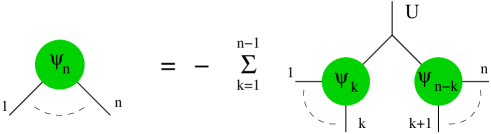
Figure 7: Tree graph expansion of the perturbative solution to the classical field equation.

This graphical representation makes it intuitively clear that the object $\langle\phi_{K},(\psi_{n}\bullet\phi_{K}+\phi_{K}\bullet\psi_{n}+\sum_{p+q=n+1}\psi_{p}\bullet\psi_{q})\rangle$ is the diagonal value of a cyclically symmetric multilinear form, since it is a ‘complete’ sum of tree graphs with $n+1$ external lines. It is possible to justify this claim by direct computation. Instead, we show cyclicity by relating $\psi_{n}$ to the products $\lambda_{n}$ used in reference [24]. To this end, we write:

$$\psi_{n}(\phi_{K}^{\otimes n})=(-1)^{n(n+1)/2}U\lambda_{n}(\phi_{K}^{\otimes n})~{}~{},$$ (B.172)

which brings (B.171) to the form:

$$\lambda_{2} = \phi_{K}\bullet\phi_{K}~{}~{}$$ (B.173)

$${\lambda}_{n} = (-1)^{n-1}\phi_{K}\bullet U{\lambda}_{n-1}+(-1)^{n-1}U{\lambda}_{n-1}\bullet\phi_{K}-\sum_{l+m=n}(-1)^{ml}U{\lambda}_{l}\bullet U{\lambda}_{m}~{}~{}{\rm for}~{}~{}n\geq 3~{}~{},$$

where we denoted $\lambda_{n}(\phi_{K}^{\otimes n})$ by $\lambda_{n}$. This coincides with the recurrence relation of [24], written for the particular case of fields with unit $U(1)$ charge. This redefinition also brings the diagrams of Figure 7 to the Feynman form, since we now have a propagator for each internal line. Equation (B) gives (for $g=1$):

$$\frac{\delta W(\phi_{K})}{\delta\phi_{K}}=-\sum_{n\geq 2}(-1)^{{1\over 2}n(n+1)}P\lambda_{n}(\phi_{K}^{\otimes n})~{}~{}.$$ (B.174)

Using the cyclicity properties of $\lambda_{n}$ discussed in [24] we find:

$$W(\phi_{K})=-\sum_{n\geq 2}{\frac{(-1)^{n(n+1)/2}}{n+1}\langle\phi_{K},\,P\lambda_{n}(\phi_{K}^{\otimes n})\rangle}=-\sum_{n\geq 3}{\frac{(-1)^{n(n-1)/2}}{n}\langle\phi_{K},\,r_{n-1}(\phi_{K}^{\otimes{n-1}})\rangle}~{}~{}.$$ (B.175)

This concludes the derivation of the potential.

References

- [1] M. R. Douglas, D-branes, Categories and N=1 Supersymmetry, hep-th/0011017.
- [2] P. S. Aspinwall, A. Lawrence, Derived Categories and Zero-Brane Stability, hep-th/0104147.
- [3] S. Hellerman, S. Kachru, A. Lawrence, J. McGreevy Linear Sigma Models for Open Strings, hep-th/0109069; S. Hellerman, J. McGreevy, Linear sigma model toolshed for D-brane physics, hep-th/0104100; K. Hori, Linear Models of Supersymmetric D-Branes, hep-th/0012179; K. Hori, A. Iqbal, C. Vafa, D-Branes And Mirror Symmetry, hep-th/0005247.
- [4] I. Brunner, M. R. Douglas, A. Lawrence, C. Romelsberger, D-branes on the Quintic, JHEP 0008 (2000) 015, hep-th/9906200.
- [5] M. R. Douglas, B. Fiol, C. Romelsberger, Stability and BPS branes, hep-th/0002037.
- [6] S. Kachru, S. Katz, A. Lawrence, J. McGreevy, Open string instantons and superpotentials, Phys.Rev. D62 (2000) 026001, hep-th/9912151; Mirror symmetry for open strings, hep-th/0006047.
- [7] M. R. Douglas, B. Fiol, C. Romelsberger, The spectrum of BPS branes on a noncompact Calabi-Yau, hep-th/0003263.
- [8] D. E. Diaconescu, M. Douglas, D-branes on Stringy Calabi-Yau Manifolds, hep-th/0006224.
- [9] P. S. Aspinwall, M. R. Douglas, D-Brane Stability and Monodromy, hep-th/0110071.
- [10] M. Alishahiha, H. Ita, Y. Oz, On Superconnections and the Tachyon Effective Action, hep-th/0012222.
- [11] Y. Oz, T. Pantev, D. Waldram, Brane-Antibrane Systems on Calabi-Yau Spaces, hep-th/0009112.
- [12] E. Witten, Topological sigma models, Commun. Math. Phys. 118 (1988),411.
- [13] E. Witten, Mirror manifolds and topological field theory, Essays on mirror manifolds, 120–158, Internat. Press, Hong Kong, 1992, hep-th/9112056.
- [14] E. Witten,Chern-Simons gauge theory as a string theory, The Floer memorial volume, 637–678, Progr. Math., 133, Birkhauser, Basel, 1995, hep-th/9207094.
- [15] C. I. Lazaroiu, Generalized complexes and string field theory, JHEP 06 (2001) 052.
- [16] C. I. Lazaroiu, Unitarity, D-brane dynamics and D-brane categories, hep-th/0102183.
- [17] D. E. Diaconescu, Enhanced D-Brane Categories from String Field Theory, hep-th/0104200.
- [18] D. Joyce, On counting special Lagrangian homology 3-spheres, hep-th/9907013.
- [19] C. I. Lazaroiu, Graded Lagrangians, exotic topological D-branes and enhanced triangulated categories, JHEP 0106 (2001) 064.
- [20] C. I. Lazaroiu, R. Roiban and D. Vaman, Graded Chern-Simons field theory and graded topological D-branes, hep-th/0107063.
- [21] P. Seidel, Graded Lagrangian submanifolds, Bull. Soc. Math. France 128 (2000), 103-149, math.SG/9903049.
- [22] A. Polishchuk, E. Zaslow, Categorical mirror symmetry: the elliptic curve, math.AG/9801119.
- [23] C. Vafa, Brane/anti-Brane Systems and Supergroup, hep-th/0101218.
- [24] C. I. Lazaroiu, String field theory and brane superpotentials, JHEP 10(2001)018, hep-th/0107162.
- [25] M. Kontsevich, Deformation quantization of Poisson Manifolds, I, mat/9709010.
- [26] S. A. Merkulov, Frobenius infinity invariants of homotopy Gerstenhaber algebras I, math.AG/0001007.
- [27] S. A. Merkulov, -algebra of an unobstructed deformation functor, math.AG/9907031
- [28] S. Barannikov, M. Kontsevich, Frobenius Manifolds and Formality of Lie Algebras of Polyvector Fields, Internat. Math. Res. Notices 4 (1998) 201–215, alg-geom/9710032.
- [29] S. Barannikov, Generalized periods and mirror symmetry in dimensions n¿3 , math.AG/9903124 ; Quantum periods - I. Semi-infinite variations of Hodge structures, math.AG/0006193; Semi-infinite Hodge structures and mirror symmetry for projective spaces, math.AG/0010157; Semi-infinite variations of Hodge structures and integrable hierarchies of KdV type, math.AG/0108148.
- [30] M. Kuranishi, Deformations of compact complex manifolds, Montreal 1971.
- [31] A. Bondal, M. M. Kapranov, Enhanced triangulated categories, Math. USSR Sbornik, vol 70 (1991) no 1, 93.
- [32] C. I. Lazaroiu, R. Roiban, to appear
- [33] J. H. Horne, Skein relations and Wilson loops in Chern-Simons gauge theory, Nucl. Phys. B334 (1990) 669; Bourdeau, E.J. Mlawer, H. Riggs and H.J. Schnitzer, The quasirational fusion structure of Chern-Simons and W-Z-W theories, Nucl. Phys. B372 (1992) 303; L. Rozansky and H. Saleur, Reidemeister torsion, the Alexander polynomial and Chern-Simons theory, J. Geom. Phys. 13 (1994) 105.
- [34] C. I. Lazaroiu, On the structure of open-closed topological field theory in two dimensions, Nucl.Phys. B603 (2001) 497-530, hep-th/0010269
- [35] J. M. Bismut and J. Lott, Flat vector bundles, direct images and higher analytic torsion, J. Amer. Math Soc 8 (1992) 291.
- [36] S. Axelrod, I. M. Singer, Chern-Simons perturbation theory, Proceedings of the XXth International Conference on Differential Geometric Methods in Theoretical Physics, Vol. 1, 2 (New York, 1991), 3–45, World Sci. Publishing, River Edge, NJ, 1992, hep-th/9110056.
- [37] K. Fukaya, Morse homotopy, -category and Floer homologies, in Proceedings of the GARC Workshop on Geometry and Topology, ed. by H. J. Kim, Seoul national University (1994), 1-102; Floer homology, -categories and topological field theory, in Geometry and Physics, Lecture notes in pure and applied mathematics, 184, pp 9-32, Dekker, New York, 1997; Floer homology and Mirror symmetry, I, preprint available at
- [38] K. Fukaya, Y.-G. Oh, H. Ohta, K. Ono, Lagrangian intersection Floer theory - anomaly and obstruction, preprint available at
- [39] W. Siegel, Fields, hep-th/9912205