BPS D3-branes on smooth
ALE manifolds^†
Talk given at the Conference New Trends in Particle Physics

September 2001, Yalta, Ukraina Pietro Fré

Dipartimento di Fisica Teorica, Universitá di Torino, $\&$ INFN - Sezione di Torino

via P. Giuria 1, I-10125 Torino, Italy

In this talk I review the recent construction of a new family of classical BPS solutions of type IIB supergravity describing 3-branes transverse to a 6-dimensional space with topology $\mathbb{R}^{2}\times$ALE. They are characterized by a non-trivial flux of the supergravity 2-forms through the homology $2$-cycles of a generic smooth ALE manifold. These solutions have two Killing spinors and thus preserve $\mathcal{N}=2$ supersymmetry. They are expressed in terms of a quasi harmonic function $H$ (the “warp factor”), whose properties was studied in detail in the case of the simplest ALE, namely the Eguchi-Hanson manifold. The equation for $H$ was identified as an instance of the confluent Heun equation.

PACS: 11.25.Hf

Keywords: 3-brane, ALE, flux

 ^† This work is supported in part by the European Union RTN contracts HPRN-CT-2000-00122 and HPRN-CT-2000-00131.

1 Introduction

After the seminal paper by Maldacena [2], many efforts have been devoted to extend the gauge/gravity correspondence to less supersymmetric and non-conformal cases. In this context considerable attention was recently directed to the study of fractional branes [3]-[16]. These are the natural elementary D-branes occurring whenever string theory is reduced on a (not necessarily compact) orbifold [17], [18]-[21]. Because of their nature they cannot move away from the orbifold apex and thus the dual gauge theory on their world-volume lacks the relevant moduli fields. Generically, this leads to both reduced supersymmetry and non-vanishing $\beta$-functions. Most interesting are the fractional D3-branes, namely the case when the world-volume theory is four-dimensional. In this respect the two most appealing situations are provided by the ${\cal N}=1$ case emerging from singular limits of CY spaces and the $\mathcal{N}=2$ case arising from the singular limit of ALE spaces. Much work was devoted to both.

A common feature of many supergravity solutions representing non-conformal situations is the presence of naked singularities of repulson type [22]. These correspond to IR singularities at the gauge theory level and one expects that they should be resolved or explained by some stringy effect. Although a general recipe does not seem to exist, progress in understanding such an issue was made both for the ${\cal N}=1$ and the $\mathcal{N}=2$ case.

In the present talk I review recent work done in collaboration with other authors [1] where it was found that the bulk solution of type IIB supergravity corresponding to fractional $D3$ can be generalized to the situation where the transverse space to the brane has a smooth regular geometry and the topology of $\mathbb{R}^{2}\,\times\,ALE$ the last factor in this product denoting a resolved Asymptotically Locally Euclidean $4$–manifold. In our solution that is shown to be supersymmetric and hence describe a BPS state of string theory there is a non zero value of the complex type IIB supergravity 3-form in the transverse directions. Note that this is the distinctive feature of fractional D-branes in the singular orbifold theories. Our bulk supergravity solution is a warped solution, but differently from the case of usual branes the warp factor depends on two rather than one radial variables and obeys a complicated partial differential equation. Actually the whole set of IIB equations can be reduced to the solution of such an equation for the warp factor, whose source is essentially dictated by supersymmetry up to an arbitrary analytic function $\gamma(z)$.

Supergravity alone is not sufficient to determine $\gamma(z)$ or the boundary conditions. This arbitrariness implies that our solution describes various deformation or various vacua of ${\cal N}=2$ theories. The case $\gamma(z)=\hbox{const.}$ describes a vanishing three-form flux and corresponds to the well known conformal ${\cal N}=2$ theory with product gauge group $\mathrm{U(N)}\times\mathrm{U(N)}$, hyper-multiplets in the bi–fundamental representation and Fayet-Iliopoulos terms describing the ALE moduli. The new ingredient in the construction of [1] is the following. It was shown how, at the supergravity level, a three-form flux can be turned on consistently with supersymmetry. Consequences of this for the dual gauge theory are the goal of a new investigation that is still ongoing.

2 Bosonic action and field equations of type IIB supergravity

As it is well known, type IIB supergravity does not have any conventional supersymmetric action. However, as it happens for all on-shell supergravity theories, the complete set of field equations can be obtained as consistency conditions from the closure of the supersymmetry transformation algebra [32]. In the case of type IIB supergravity, one was also able [33] to obtain a complete, manifestly $\mathrm{SU(1,1)}$-covariant formulation of the theory based on the rheonomic approach to supergravity theory [34].

The bosonic part of the equations can be formally obtained through variation of the following action :

$$S_{\rm IIB}=\frac{1}{2\kappa^{2}}\Bigg{\{}\int d^{10}x~{}\left[-2\sqrt{-\det g}~{}R\right]-\frac{1}{2}\int\Big{[}d\varphi\wedge\star d\varphi\,+\,{\rm e}^{-\varphi}F_{[3]}^{NS}\wedge\star F_{[3]}^{NS}\,+\,{\rm e}^{2\varphi}\,F_{[1]}^{RR}\wedge\star F_{[1]}^{RR}$$

$$+\,\,{\rm e}^{\varphi}\,{F}_{[3]}^{RR}\wedge\star{F}_{[3]}^{RR}\,+\,\frac{1}{2}\,{F}_{[5]}^{RR}\wedge\star{F}_{[5]}^{RR}\,-\,C_{[4]}\wedge F_{[3]}^{NS}\wedge F_{[3]}^{RR}\Big{]}\Bigg{\}}$$ (2.1)

where:

$$\begin{array}[]{cclcccl}F^{RR}_{[1]}&=&dC_{[0]}&;&F^{NS}_{[3]}&=&dB_{[2]}\\ F^{RR}_{[3]}&=&dC_{[2]}-\,C_{[0]}\,dB_{[2]}&;&F^{RR}_{[5]}&=&dC_{[4]}-{\textstyle\frac{1}{2}}\left(B_{[2]}\wedge dC_{[2]}-C_{[2]}\wedge dB_{[2]}\right)\end{array}$$ (2.2)

It is important to stress though that the action (2.1) is to be considered only a book keeping device since the $4$-form $C_{[4]}$ is not free, its field strength $F_{[5]}^{RR}$ being subject to the on-shell self-duality constraint:

$$F_{[5]}^{RR}=\star F_{[5]}^{RR}$$ (2.3)

¿From the above action the corresponding equations of motion can be obtained:

$$d\star d\varphi-e^{2\varphi}\,F^{RR}_{[1]}\wedge\star F^{RR}_{[1]} = -{\textstyle\frac{1}{2}}\,\left(e^{-\varphi}F^{NS}_{[3]}\wedge\star F^{NS}_{[3]}-e^{\varphi}F^{RR}_{[3]}\wedge\star F^{RR}_{[3]}\right)$$ (2.4)

$$d\left(e^{2\varphi}\star F^{RR}_{[1]}\right) = -e^{\varphi}\,F^{NS}_{[3]}\wedge\star F^{RR}_{[3]}$$ (2.5)

$$d\left(e^{-\varphi}\,\star F_{[3]}^{NS}\right)+e^{\varphi}\,F^{RR}_{[1]}\wedge\star F^{RR}_{[3]} = -F_{[3]}^{RR}\wedge F^{RR}_{[5]}$$ (2.6)

$$d\left(e^{\varphi}\star F_{[3]}^{RR}\right) = -F_{[5]}^{RR}\,\wedge F_{[3]}^{NS}$$ (2.7)

$$d\star F^{RR}_{[5]} = -F^{NS}_{[3]}\,\wedge\,F^{RR}_{[3]}$$ (2.8)

$$-\,2\,R_{{MN}} = \frac{1}{2}\partial_{{M}}\varphi\partial_{{N}}\varphi+\frac{e^{2\varphi}}{2}\partial_{{M}}C_{[0]}\partial_{{N}}C_{[0]}+150{F}_{[5]{M}\cdot\cdot\cdot\cdot}{F}_{[5]{N}}^{\phantom{{M}}\cdot\cdot\cdot\cdot}$$ (2.9)

$$+9\left(e^{-\varphi}F_{[3]{M}\cdot\cdot}^{NS}\,F_{[3]{N}}^{{NS}\phantom{{M}}\cdot\cdot}+e^{\varphi}{F}_{[3]{M}\cdot\cdot}^{RR}{F}_{[3]{N}}^{RR\phantom{{M}}\cdot\cdot}\right)$$

$$-\frac{3}{4}\,g_{{MN}}\,\left(e^{-\varphi}F_{[3]\cdot\cdot\cdot}^{NS}F_{[3]}^{NS\cdot\cdot\cdot}+e^{\varphi}{{F}}_{[3]\cdot\cdot\cdot}^{RR}{F}^{RR\cdot\cdot\cdot}_{[3]}\right)$$

It is not difficult to show, upon suitable identification of the massless superstring fields, that this is the correct set of equations which can be consistently obtained from the manifestly $\mathrm{SU(1,1)}$ covariant formulation of type IIB supergravity [33].

3 $D3$-brane solution with ALE flux

In this section we provide the BPS solution corresponding to a 3-brane transverse to a smooth ALE space, namely we construct type IIB supergravity solutions describing 3 branes on a vacuum $\mathbb{R}^{1,3}\times\mathbb{R}^{2}\times\mathrm{ALE}$. This will be achieved without an analysis of the specific form of the world-volume action of the brane, i.e. of the source term. Our physical assumption will just be that, together with the usual RR 5-form flux, the 3-brane solution has a non-trivial flux of the supergravity 2-form potentials along (one of) the compact two cycle(s) of the blown-up orbifold (this translates into a non-vanishing value of the complex 3-form field strength).

3.1 Solution of the bosonic field equations

We separate the ten coordinates of space-time into the following subsets:

$$x^{M}=\left\{\begin{array}[]{rcll}&x^{\mu}\quad\mu=0,1,2,3&\mbox{coordinates of the 3-brane world volume}\\ &z\;=\;x^{4}+{\rm i}x^{5}&\mbox{complex coordinate of $\mathbb{R}^{2}\sim\mathbb{C}$}\hbox{}\\ &y^{\tau}\quad\tau=6,7,8,9&\mbox{real coordinates of the ALE 4-space }\end{array}\right.$$ (3.1)

and we make the following ansatz for the metric:

$$ds^{2}=H^{-\frac{1}{2}}\left(-\eta_{\mu\nu}dx^{\mu}\,dx^{\nu}\right)+H^{\frac{1}{2}}dzd\bar{z}+H^{\frac{1}{2}}ds^{2}_{ALE}$$ (3.2)

where the warp factor $H=H(z,\bar{z},y)$ depends in principle on all the transverse variables and $ds^{2}_{ALE}=g^{ALE}_{\tau\sigma}dy^{\tau}\,dy^{\sigma}$ is the metric of any ALE space and we denote $M_{6}=\mathbb{R}^{2}\times\mathrm{ALE}$ the six-manifold spanned by $z$, $\bar{z}$ and $y^{\tau}$. Defining ${\mathcal{H}}_{\pm}=\pm 2\,e^{-\varphi/2}F^{NS}_{[3]}+{\rm i}2\,e^{\varphi/2}\,F^{RR}_{[3]}$, eq. (2.8) for the 5-form becomes:

$$d\star F^{RR}_{[5]}={\rm i}\,{\textstyle\frac{1}{8}}\,{\mathcal{H}}_{+}\wedge{\mathcal{H}}_{-}$$ (3.3)

Besides assuming the structure (3.2) we also assume that the two scalar fields, namely the dilaton $\varphi$ and the Ramond-Ramond $0$-form $C_{[0]}$ are constant and vanishing $\varphi=0\,;\,C_{[0]}=0$. This assumption simplifies considerably the equations of motion.

The basic ansatz characterizing our solution and providing its interpretation as a 3-brane with a flux through a homology 2-cycle of the ALE space is given by the following:

$$\begin{array}[]{ccccccc}{\mathcal{H}}_{+}&=&2\,d\gamma_{I}(z,{\bar{z}})\,\wedge\,\omega^{I}&;&{\mathcal{H}}_{-}&=&-2\,d{\bar{\gamma}_{I}}(z,{\bar{z}})\,\wedge\,\omega^{I}\end{array}$$ (3.4)

where $\gamma_{I}(z,{\bar{z}})$ is a complex field depending only on the coordinates $z,\bar{z}$ of $\mathbb{R}^{2}$, while $\omega^{I}$ ($I=1,\dots,k$) constitute a basis for the space of square integrable, anti-self-dual, harmonic forms on the ALE manifold.

As it is well known a smooth ALE manifold, arising from the resolution of a $\mathbb{C}^{2}/\Gamma$ singularity, where $\Gamma\subset\mathrm{SU(2)}$ is a discrete Kleinian group, has Hirzebruch signature:

$$\tau=\left(\#\mbox{of conjugacy classes of $\Gamma$}\right)-1=\mbox{rank of }\,\mathbb{G}(\Gamma)$$ (3.5)

In the above formula $\mathbb{G}(\Gamma)$ is the simply laced Lie algebra corresponding to $\Gamma$ in the ADE classification of Kleinian groups, based on the Mac Kay correspondence [36]. As a result of eq.(3.5) the ALE manifold that is HyperKähler admits a triplet of self-dual $2$-forms that are non-integrable and exactly $\tau$ integrable anti-self-dual harmonic $2$-forms. For these latter one can choose a basis $\omega^{I}$ that is dual to the integral homology basis of $2$-cycles $\Sigma_{I}$ whose intersection matrix is the Cartan matrix $\mathcal{C}$ of $\mathbb{G}(\Gamma)$. Explicitly we can write:

$$\begin{array}[]{ccccccccccc}\int_{\Sigma_{K}}\,\omega^{I}&=&\delta^{I}_{K}&;&\int_{ALE}\omega^{I}\wedge\omega^{J}&=&-\,{\cal C}^{-1\,IJ}&;&\omega^{I}\wedge\omega^{J}&=&-\,\Delta^{IJ}(y)\,\Omega_{ALE}\\ \end{array}$$ (3.6)

where ${\cal C}^{IJ}$ is the Cartan matrix of the corresponding (non-extended) ADE Dynkin diagram and $\Delta^{IJ}(y)$ is a positive definite matrix whose entries are functions of the ALE space coordinates $y$’s. The anti-self-duality of the $\omega^{I}$ guarantees that $\int\omega^{I}\wedge\star\omega^{J}$ is positive definite. If we insert our ansätze into the scalar field equations (2.4, 2.5) we obtain ${\mathcal{H}}_{+}\,\wedge\,\star{\mathcal{H}}_{+}=0$ which in turn implies that $\partial_{z}\gamma_{I}\,\bar{\partial}_{\bar{z}}\gamma_{J}=0$. This equation is solved by choosing $\gamma_{I}$ to be holomorphic: $\bar{\partial}\gamma_{I}=0$ where $\partial=dz\,\frac{\partial}{\partial z}$, ${\bar{\partial}}=d{\bar{z}}\,\frac{\partial}{\partial{\bar{z}}}$. Next we consider the self-dual $5$-form $F_{[5]}^{RR}$ which, because of its definition, must satisfy the following Bianchi identity: $d\,F_{[5]}^{RR}={\rm i}\,{\textstyle\frac{1}{8}}\,{\mathcal{H}}_{+}\,\wedge\,{\mathcal{H}}_{-}$. Our ansatz for $F_{[5]}^{RR}$ is the following: ( $\Omega$ are the volume forms)

$$F_{[5]}^{RR}=\alpha\left(U+\star U\right)\quad;\quad U=d\left(H^{-1}\,\Omega_{\mathbb{R}^{1,3}}\right)$$ (3.7)

where $\alpha$ is a constant to be determined later. By construction $F_{[5]}^{RR}$ is self-dual and its equation of motion is trivially satisfied. What is not guaranteed is that also the $5$–form Bianchi identity is fulfilled. Imposing it, results into a differential equation for the function $H(z,\bar{z},y)$:

$$\left(\square_{\mathbb{R}^{2}}+\square_{ALE}\right)H=-\frac{1}{\alpha}\partial_{z}\gamma_{I}\,\partial_{\bar{z}}{\bar{\gamma}}_{J}\,\Delta^{IJ}(y)$$ (3.8)

This is the main differential equation the entire construction of our sought for 3-brane solution can be reduced to. The parameter $\alpha$ is determined by Einstein’s equation and fixed to $\alpha=1$.

The field equation for the complex three-form, namely eq.s (2.6) and (2.7) reduces to: ${\bar{\partial}}\wedge\partial\gamma_{I}=0\,\Rightarrow\,\square_{\mathbb{R}^{2}}\gamma_{I}=0$. This equation has to be appropriately interpreted. It says that $\gamma_{I}$ are harmonic functions in two-dimensions as the real and imaginary parts of any holomorphic function $\gamma_{I}(z)$ certainly are. The bulk equations do not impose any additional constraint besides this condition of holomorphicity. However, in presence of a boundary action for the $3$ brane, the equation will be modified into:

$$\square_{\mathbb{R}^{2}}\gamma_{I}=j_{I}(z)$$ (3.9)

$j_{I}(z)$ being a source term, typically a delta function. In this case $\gamma_{I}$ is fixed as: $\gamma_{I}(z)=\int\,G_{\mathbb{R}^{2}}(z,z^{\prime})\,j_{I}(z^{\prime})\,dz^{\prime}$ where $G_{\mathbb{R}^{2}}(z,z^{\prime})$ is the Green function of the $\mathbb{R}^{2}$ Laplacian in complex coordinates and turns out to be proportional to $\log z$.

3.2 Proof of bulk supersymmetry

As usual, in order to investigate the supersymmetry properties of the bosonic solution we have found it suffices to consider the supersymmetry transformation of the fermionic fields (the gravitino and the dilatino) and impose that, for a Killing spinor, they vanish identically on the chosen background. By using the formulation of [33], one easily gets:

$$\delta\psi_{M} = \mathcal{D}_{M}\chi+{\textstyle\frac{1}{16}}\,{\rm i}\Gamma^{A_{1}\dots A_{5}}\,F_{A_{1}\dots A_{5}}\,V^{B}_{M}\,\Gamma_{B}\,\chi\,$$

$$+{\textstyle\frac{1}{32}}\left(-\Gamma_{BA_{1}\dots A_{3}}\,V^{B}_{M}+9\Gamma^{A_{1}A_{2}}V^{A_{3}}_{M}\right)\,{\mathcal{H}}_{+|A_{1}A_{2}A_{3}}\,\chi^{\star}$$

$$\delta\,\lambda = -{\rm i}\,{\textstyle\frac{1}{8}}\,\Gamma^{A_{1}A_{2}A_{3}}\,{\mathcal{H}}_{+|A_{1}A_{2}A_{3}}\,\chi$$ (3.10)

where the supersymmetry parameter $\chi$ is a complex ten-dimensional Weyl spinor, $\Gamma_{11}\,\chi=\chi$ and where we have already used the information that on our background the dilaton and the Ramond scalar vanish. To analyze supersymmetry on such a background the appropriate gamma matrix basis $\left(\left\{\Gamma^{A}\,,\,\Gamma^{B}\right\}=\eta^{AB}\right)$ is the following:

$$\Gamma^{A} = \left\{\begin{array}[]{rcl}\Gamma^{a}&=&\gamma^{a}\,\otimes{\bf 1}\\ \Gamma^{i}&=&\gamma_{5}\,\otimes\,\tau^{i}\end{array}\right.$$ (3.13)

where $\left\{\gamma^{a}\,,\,\gamma^{b}\right\}=2\,\eta^{ab}$ , $\gamma_{5}=-{\rm i}\gamma^{0}\gamma^{1}\gamma^{2}\gamma^{3}$, $\left\{\tau^{i}\,,\,\tau^{j}\right\}=2\,\eta^{ij}=-2\,\delta^{ij}$ , $\tau_{\bullet}=-\tau^{4}\tau^{5}\tau^{6}\tau^{7}\tau^{8}\tau^{9}$ are the gamma matrices in Lorentzian four space and on the six dimensional manifold $M_{6}$ respectively. Then the $\tau^{i}$ matrices are further decomposed with respect to the submanifolds $\mathbb{R}^{2}$ and $\mathrm{ALE}$ as it follows:

$$\tau^{i}=\left\{\begin{array}[]{rcl}\tau^{\alpha}&=&{\rm i}\sigma^{\alpha}\,\otimes\,{\bf 1}\\ \tau_{u}&=&{\rm i}\sigma^{3}\,\otimes\,\overline{\gamma}_{u}\end{array}\right.$$ (3.14)

where $\sigma^{\alpha}=\sigma^{1,2}$ and $\sigma^{3}$ are the standard Pauli matrices while $\left\{\overline{\gamma}_{u}\,,\,\overline{\gamma}_{v}\right\}=\delta_{uv}$ are $4\times 4$ hermitian matrices forming an Euclidean realization of the four-dimensional Clifford algebra. Writing the $32$-component spinor $\chi$ as a tensor product:

$$\chi=\varepsilon\,\otimes\,\eta$$ (3.15)

of a $4$-component spinor $\varepsilon$, related to the $3$-brane world volume with an $8$-component spinor $\eta$ related to the transverse manifold $M_{6}$, the transformations of the gravitino and dilatino (3.10) vanish if:

$$\begin{array}[]{lclclcl}\partial_{a}\,\varepsilon=0&;&\gamma_{5}\,\varepsilon=\varepsilon&;&\eta=H^{-1/8}(z,\bar{z},y)\,\theta\,\otimes\,\xi&;&0=\widehat{\mathcal{D}}\xi\\ \overline{\gamma}_{5}\xi_{-}=-\xi_{-}&;&\sigma_{3}\,\theta\,=-\theta&;&0=\partial_{z}\theta&;&0=\partial_{\bar{z}}\theta\end{array}$$ (3.16)

The specific geometric properties of the ALE manifold play at this point an essential role. The integrability condition for covariantly constant spinors $\xi$ is, as usual given by $-{\textstyle\frac{1}{4}}\,R^{uv}\,\overline{\gamma}_{uv}\,\xi=0$ where $R^{uv}\,\overline{\gamma}_{uv}$ is the curvature $2$-form of the ALE manifold. This latter is HyperKähler and as such it has a triplet of covariantly constant self-dual $2$-forms $\Omega^{x}$, $(x=1,2,3)$ whose intrinsic components satisfy the quaternionic algebra. This implies that the holonomy of the manifold is $\mathrm{SU(2)}_{L}$ rather than $\mathrm{SO(4)}=\mathrm{SU(2)_{L}}\times\mathrm{SU(2)_{R}}$ and that the curvature $2$-form is anti-self-dual. This follows from the integrability condition for the covariant constancy of the self-dual HyperKähler $2$-forms. On the other hand, from the Hirzebruch signature $\tau$ of the ALE manifold it follows that there are exactly $\tau$ normalizable anti-self-dual forms $\omega_{I}$. From the trivial gamma matrix identity $\overline{\gamma}_{5}\,\overline{\gamma}_{uv}=-{\textstyle\frac{1}{2}}\,\epsilon_{uvst}\,\overline{\gamma}^{st}$ follows that the two chirality eigenspaces: $\overline{\gamma}_{5}\xi_{\pm}=\pm\xi_{\pm}$ are respectively annihilated by the contraction of $\overline{\gamma}_{uv}$ with any self-dual or anti self-dual $2$-form. Therefore antichiral spinors $\xi=\xi_{-}$ satisfy the integrability condition automatically . Once this condition is fulfilled, the equation $\widehat{D}_{a}\xi=0$ can be integrated yielding two linear independent solutions $\xi_{-}^{1,2}$ that span the irreducible representation $(0,1/2)$ of $\mathrm{SO(4)}$. The other irreducible representation $(1/2,0)$ corresponds to spinors that are not Killing and do not generate supersymmetries preserved by the background. In conclusion we have $2$ Killing spinors generating an $\mathcal{N}=2$ supersymmetry on the world volume. In other words the bosonic background we have constructed corresponds to a BPS state preserving a total of $2\times 4=8$ supercharges.

4 The Eguchi-Hanson case

As showed above, the complete integration of the supergravity field equations is reduced to the solution of a single differential equation, namely eq. (3.8). It is worth to investigate the properties of such an equation, choosing the simplest instance of an ALE manifold, namely the Eguchi-Hanson space [37], which in the ADE classification corresponds to $A_{1}\sim\mathbb{Z}_{2}$. In paper [1] a complete and detailed mathematical analysis of such a case was given. In this talk I summarize the main results of such an analysis. It should be stressed that, whereas the results of the previous sections were entirely based on type IIB supergravity, in what follows we have to make some reasonable assumptions on the nature of the microscopic theory, namely the structure of the source terms needed to fix the boundary conditions.

The Eguchi-Hanson metric has the form:

$$ds^{2}_{EH}=g(r)^{-2}\,dr^{2}+r^{2}\,\left(\sigma_{x}^{2}+\sigma_{y}^{2}\right)+r^{2}\,g(r)^{2}\,\sigma_{z}^{2}\quad;\quad g(r)^{2}=1-\left(\frac{a}{r}\right)^{4}$$ (4.1)

where $r\geq a$, $\theta\in\left[0,\,\pi\right[$ and $\psi$, $\phi\in\left[0,\,2\pi\right[$. The $1$-forms $\sigma^{i}=\left\{\sigma^{x},\,\sigma^{y},\,\sigma^{z}\right\}$ satisfy, by definition the Maurer Cartan equations of $SO(3)$ and are defined on the three sphere.

This space has a unique homology 2-cycle $\Sigma$ located at $r=a$ and spanned by the coordinates $\theta$, $\phi$. The anti-self dual form $\omega$ fulfilling eqs. (3.6) is:

$$\omega = \frac{a^{2}}{2\,\pi}\,d\left(\frac{\sigma_{z}}{r^{2}}\right)$$ (4.2)

The function $\Delta(y)$ defined in (3.6) is explicitly evaluated to be:

$$\Delta(y) = \frac{2\,a^{4}}{\pi^{2}\,r^{8}}$$ (4.3)

The equation for $H$ in the Eguchi-Hanson case can then be easily obtained from the general expression in eq.(3.8). As it is usually the case, we make a spherically symmetric ansatz, compatible with the background at hand: for the case we shall be interested in, the coefficients of the equation for $H$ depend only on the radial coordinates $\rho=\sqrt{z\bar{z}}$ and $r$ on $\mathbb{R}^{2}$ and on the Eguchi-Hanson space respectively, and we can then assume the same property for $H$ to hold and write it as $H(\rho,\,r)$. The equation for $H$ can then be written as:

$$\left(\partial_{4}^{2}+\partial_{5}^{2}\right)\,H+\frac{1}{r^{3}}\partial_{r}\left(r^{3}\,g(r)^{2}\,\partial_{r}H\right) = -\frac{2\,a^{4}}{\pi^{2}\,r^{8}}\,|\partial_{z}\,\gamma|^{2}+{\cal S}(\rho,\,r)$$ (4.4)

where ${\cal S}(\rho,\,r)$ is a source term for the $3$-brane charge for which we also make a spherical ansatz. Differently from the first term on the right hand side, ${\cal S}(\rho,\,r)$ is not deduced from the dynamics in the bulk. In the present analysis its presence should be intended only for the sake of fixing boundary conditions near the cycle.

The best technique to study eq.(4.4) is that of performing a Bessel–Fourier transform. For convenience we choose to study the equation in the Fourier transform $\widetilde{H}(\mu,r)$ of $H(\rho,r)-1$ instead of $H(\rho,r)$. In this way the boundary conditions at infinity: $H(\rho,r)\,\rightarrow\,1$ is automatically implemented if $\widetilde{H}(\mu,r)\,\rightarrow\,0$. The relation between $\widetilde{H}(\mu,r)$ and $H(\rho,r)$ is given by: $\widetilde{H}(\mu,r)=\frac{1}{2\pi}\int_{0}^{\infty}d\rho\,\rho\,J_{0}(\mu\rho)\,\left(H(\rho,r)-1\right)$. The equation for $\widetilde{H}(\mu,\,r)$ has the following form:

$$\left[\frac{1}{r^{3}}\frac{d}{dr}\,\left(r^{3}\,g(r)^{2}\,\frac{d}{dr}\right)-\mu^{2}\,\right]\,\widetilde{H}(\mu,\,r)=J(\mu,\,r)$$ (4.5)

where we have defined the source function: $J(\mu,\,r)\,\equiv\,-\frac{2a^{4}}{\pi^{2}\,r^{8}}\,j(\mu)+S(\mu,\,r)$. The symbol $j(\mu)$ denotes the Fourier transform of $|\partial\gamma(z)|^{2}$ while $S(\mu,\,r)$ is the transform of the source term ${\cal S}(\rho,\,r)$ for the $3$-brane charge.

It is known from the standard theory of differential equations that the general integral $\widetilde{H}(\mu,\,r)$ of eq. (4.5) has the form:

$$\widetilde{H}(\mu,\,r)=\beta_{1}\,u_{1}(\mu,\,r)+\beta_{2}\,u_{2}(\mu,\,r)+u_{n-h}(\mu,\,r)$$ (4.6)

where $u_{1,2}(\mu,\,r)$ are two independent solutions of the homogeneous equation associated with (4.5).

4.1 The $3$-brane charge and the physical boundary conditions

The physical boundary conditions for the $D3$–brane solution are imposed by selecting the asymptotic behaviour of the warp factor $H$ near infinity $r\to\infty$ and near the cycle at $r\to a$. In order to perform such an analysis we just need to consider the two asymptotic limits $r\to\infty$ and $r\to a$ of the Eguchi Hanson metric. As for the limit $r\to\infty$ the limit is clear, the Eguchi Hanson metric approaches the flat metric and this is just what ALE means, namely asymptotically locally Euclidean. The near cycle limit of the same metric metric (4.1) is exposed by performing the following change of variable: $r\rightarrow v=\frac{{\sqrt{r^{4}-a^{4}}}}{2\,r}$. By expanding the metric (4.1) in power series of $v$ at $v=0$ which corresponds to $(r\to a)$, we obtain:

$$ds^{2}_{EH} \simeq_{v\to 0} dv^{2}+v^{2}\,d\psi^{2}+\frac{a^{2}}{4}\,\left(d\theta^{2}\,+\,d\phi^{2}\,\sin^{2}\theta\right)+\mathcal{O}\left(v^{2}\right)$$ (4.7)

showing that near the homology cycle the Eguchi-Hanson metric approximates that of a manifold $\mathbb{R}^{2}\,\times\,\mathrm{S}^{2}$.

Equipped these results, let us now consider the case of a $3$-brane with vanishing 3-form placed either at the origin of $\mathbb{R}^{6}$ in the orbifold case where the transverse space is $M_{6}=\mathbb{R}^{2}\times\mathbb{R}^{4}/\Gamma$ or at the homology cycle $r=a$ in the case where the transverse space is $M_{6}=\mathbb{R}^{2}\times\mathrm{ALE_{EH}}$. Naming $Q$ the charge of such a brane, the expected behavior of the $H$ function near the brane is, in the two cases, the following one:

$$H\simeq\frac{Q}{(x_{4}^{2}+x_{5}^{2}+\dots+x_{9}^{2})^{2}}\quad\mbox{for $\mathbb{R}^{6}$; }\quad H\simeq\frac{Q/{2a^{2}}}{\,(\rho^{2}+v^{2})}\quad\mbox{for $\mathbb{R}^{2}\times$ ALE }$$ (4.8)

The first of eq.s (4.8) is obvious. The second is due to the discussion of the previous section. Near the cycle the Laplacian on $M_{6}$ becomes $\square_{M_{6}}\sim\square_{\mathbb{R}^{4}}+\square_{S^{2}}$ and since $S^{2}$ is a compact, positive curvature manifold there are no zero modes of $\square_{S^{2}}$ except the constant. Therefore the non trivial part of $H$ behaves as a harmonic function on $\mathbb{R}^{4}$, namely the second of eq.s (4.8). The scale factor $1/(a^{2})$ appearing there is understood as follows. If $Q$ is the total charge perceived at infinity, the density of charge on the homology $2$-sphere of radius $\frac{a}{2}$ is: $q=\frac{Q}{a^{2}\pi}$. Hence what appears as charge in the near cycle $\mathbb{R}^{4}$ plane is $q$ rather than $Q$. Finally the $\pi/2$ factor that is needed to match the second with the first of equations (4.8) is just a matter of convenient normalization. Let us now perform the Fourier-Bessel transform of eq.s (4.8). We obtain

$$\frac{1}{2\pi}\,\int_{0}^{\infty}\,J_{0}(\mu\,\rho)\,\rho\,\frac{Q}{(r^{2}+\rho^{2})^{2}}\,d\rho = \frac{Q}{4\pi}\,\frac{\mu}{r}\,K_{1}\left(\mu\,r\right)$$

$$\frac{1}{2\pi}\,\int_{0}^{\infty}\,J_{0}(\mu\,\rho)\,\rho\,\frac{Q}{2a^{2}\,\left(v^{2}+\rho^{2}\right)}d\rho = \frac{Q}{4\pi}\,\frac{1}{a^{2}}\,K_{0}\left(\mu\,v\right)$$ (4.9)

The important conclusion implied by the above analysis is that we have obtained the physically appropriate boundary conditions for the function $\widetilde{H}(\mu,r)$. In both the orbifold or smooth ALE case, in the limits $r\rightarrow 0$ and $r\rightarrow a$ respectively, we have: $\widetilde{H}(\mu,r)\sim\frac{Q}{4\pi}{u}^{div}_{1}(\mu,\,r)+\mbox{reg}$ where $Q$ is the $3$-brane charge and ${u}^{div}_{1}(\mu,\,r)$ denotes the divergent part of that of the two solutions $u_{1,2}(a,\,\mu,\,r)$ of the homogeneous Laplacian equation that is divergent in the limit. This condition, together with the boundary condition at infinity, fixes the coefficients $\beta_{1},\,\beta_{2}$ in eq. (4.6) to be: $\beta_{1}=\frac{Q}{4\pi}\,;\,\beta_{2}=0$. The appropriate source for such boundary conditions is: $S(\mu,\,r)=-\frac{Q}{2\pi}\,\frac{\delta(r-a)}{r^{3}}$. From the physical viewpoint this source term comes from the world-volume action of the $D3$-brane.

4.2 Reduction to the confluent Heun equation

As we have seen in previous sections a convenient approach to the solution of equation (4.4) relies on the partial Fourier transform leading to the new eq. (4.5), for the function $\widetilde{H}(\mu,r)$. In [1] it was shown that complete equation reduces to a confluent form of the Heun equation. This is obtained by parameterizing the radial direction in the Eguchi-Hanson space through the new variable $w=(a^{2}-r^{2})/(2a^{2})$ so that the main differential equation (4.5) can be rewritten in the following form:

$$w^{2}\,\frac{d^{2}\widetilde{H}}{dw^{2}}+w\,P_{1}(w)\,\frac{d\widetilde{H}}{dw}+P_{2}(\mu,\,w)\,\widetilde{H} = \frac{h(\mu)\,w}{(1-w)(1-2w)^{3}}$$

$$\widetilde{H}(\mu,w) \stackrel{{\scriptstyle w\rightarrow-\infty}}{{\longrightarrow}} 0$$ (4.10)

where $P_{1}(w)=\frac{2w-1}{w-1}$, $P_{2}(\mu,\,w)=k\,w\,\left(\frac{2w-1}{w-1}\right)$, $h(\mu)=\frac{1}{2\pi^{2}\,a^{2}}\,j(\mu)$ =$\frac{1}{2\pi^{2}a^{2}}\int_{0}^{\infty}\,\frac{d^{2}x}{(2\pi)^{2}}\,|\partial_{z}\gamma(z)|^{2}\,e^{{\rm i}\vec{p}\cdot\vec{x}}$, $k=\frac{\mu^{2}a^{2}}{4}$. In the source term we omit the part proportional to $S(\mu,\,r)$ since, as just explained its effect amounts to a determination of the relative coefficients of the two independent solutions $u_{1,2}$ of the homogeneous equation.

The power series solution of eq.(4.10) explicitly discussed in [1] is a smooth interpolation between the two asymptotic behaviours of the warp factor that we recall here in complete form. Far away from the cycle we have:

$$\left(\rho,r\gg a\right):\quad H(\rho,\,r)\sim\frac{Q}{(\rho^{2}+r^{2})^{2}}\left(1+\mathrm{log~{}terms}\right)$$ (4.11)

while in the region near the cycle, combining the asymptotic behaviors of the homogeneous and inhomogeneous solutions, we find

$$\left(\matrix{\rho<a\cr r\sim a}\right):\quad H(\rho,\,r)\sim\frac{Q}{2a^{2}}\frac{1}{\rho^{2}+v^{2}}-\frac{1}{2\pi^{2}\,a^{4}}\,K\,\log{\left(\frac{\rho}{\rho_{0}}\right)}^{2}$$ (4.12)

where $K$ is a constant, completely free at the level of the bulk supergravity analysis. The corrections to the above behavior can be systematically deduced from the power series expansion of the solution described in [1]. Looking at eq.(4.12), it is clear that there could be a value of $r,\rho$ for which $H=0$, this being an indication for the presence of a naked singularity of the repulson type [22]. This singularity should be removed, somehow. In most non-conformal $\mathcal{N}=2$ versions of the gauge/gravity correspondence this singularity has been shown to be excised by the so-called enhançon mechanism [24]. This is the case, for instance, of fractional branes on orbifolds, [8], [17]. The value of the enhançon corresponds to $\rho=\rho_{e}$, the scale where the scalar field $\gamma$ vanishes. This in general turns out to be the scale where the dual gauge theory becomes strongly coupled and new light degrees of freedom are expected to become relevant, both at the gauge theory (where instanton effects become important) and at the supergravity level (where tensionless strings occur). For all this analysis to work, it is important that $\rho_{e}$ is bigger than the scale at which the repulson occurs. In fact, when this is the case, the region where supergravity is reliable, namely $\rho>\rho_{e}$, is free of any singularity. In order to see if this happens also in our case and if the cut-off $\rho_{e}$ has in fact the expected meaning, one should have a full control on the world-volume action of the source. However the solution I have presented differs from that of fractional branes on singular space because of the improved behaviour of the warp factor $H$ on the plane $\mathbb{R}^{2}$ where it is non-singular, while the solution of the field $\gamma$, which is responsible for the enhançon mechanism, has essentially the same structure. Hence this bulk solution is reliable, well-defined and singularity free for $\rho>\rho_{e}$ where the leading order near cycle behaviour is well described by the first term in eq. (4.12).

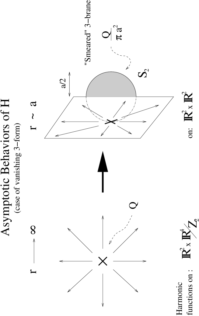
Figure 1:

5 Final considerations on the metric and open problems

Introducing the variable $R=\sqrt{(\rho^{2}+v^{2})}$ that measures the radial coordinate of $\mathbb{R}^{4}$ in units of $q$ we find that near the cycle we have $H\sim q/R^{2}$, yielding

$$ds^{2}\sim\frac{R}{\sqrt{q}}(-\eta_{\mu\nu}dx^{\mu}dx^{\nu})+\frac{\sqrt{q}}{R}dR^{2}+\sqrt{q}Rds^{2}_{\mathbf{S}^{3}}+\frac{\sqrt{q}}{R}\frac{a^{2}}{4}ds^{2}_{\mathbf{S}^{2}}$$ (5.1)

where $ds^{2}_{\mathbf{S}^{2}}$ is the metric of the two cycle of Eguchi-Hanson and $ds^{2}_{\mathbf{S}^{3}}$ is the metric of the three-sphere at fixed $R$ in $\mathbb{R}^{4}$. An interesting point is that the above result holds even in the absence of the three-form flux and shows that conformal invariance of the dual theory is always broken since the metric in $R$ and $x^{\mu}$ is no longer of anti de Sitter type. Obviously we cannot take the limit $R\to 0$ since this would imply going to large curvatures, and in particular crossing the enhançon radius. However, the result suggests that a possible interpretation for the parameter $a$ in the Eguchi-Hanson metric is that of a Fayet Iliopoulos term, breaking conformal invariance in the infrared, in accord with previous work on the subject.

The situation can be summarized as follows. In the absence of flux the exact supersymmetric $D3$-brane solution that we have found interpolates between a standard ten dimensional $D3$-brane solution at the singularity of the metric cone on $S^{5}$, i.e. the standard $\mathbb{R}^{6}$ manifold, and a $D3$-brane solution of an effective $8$-dimensional supergravity. The interpolation mechanism is described in fig. 1. As explained in the literature [39] (for a review see [40]) we can always consider sphere reductions of all supergravity theories and in particular an $S^{2}$-reduction of type IIB supergravity. This yields an effective $8$-dimensional supergravity that has $3$-brane solutions. In this case however, there is a coupling to an effective dilaton that emerges as the conformal factor of the metric in the dimensional reduction. Hence the $D3$-brane solution of the $8$-dimensional supergravity is no longer conformal and we can follow the prescription of Townsend et al [41] by making the transition to a dual frame where the metric factorizes into the product of a $3$-sphere metric times a domain wall solution of an effective five-dimensional supergravity theory.

Investigating the relation with the effective $8$–dimensional supergravity and the properties of the dual gauge theory on the world volume are the challenging open problems posed by the type IIB solution I have described in this talk.

Acknowledgments It is my pleasure to thank my collaborator and friend Mario Trigiante for help in preparing this talk and all the coauthors of paper [1] on which what I told is entirely based.

References

- [1] M. Bertolini, V.L. Campos, G. Ferretti, P. Fré, P. Salomonson, M. Trigiante. Supersymmetric 3–branes on smooth ALE manifolds with flux hep-th/0106186, to appear on Nucl. Phys.
- [2] J. Maldacena, The large N limit of superconformal field theories and supergravity, Adv. Theor. Math. Phys. 2 (1998) 231, hep-th/9711200.
- [3] I. R. Klebanov and N. A. Nekrasov, Gravity duals of fractional branes and logarithmic RG flow, Nucl. Phys. B574 (2000) 263, hep-th/9911096.
- [4] I.R. Klebanov and A.A. Tseytlin, Gravity duals of supersymmetric SU(N)*SU(N+M) gauge theories, Nucl. Phys. B578 (2000) 123, hep-th/0002159.
- [5] K. Oh and R. Tatar, Renormalization group flows on D3 branes at an orbifolded conifold, JHEP 05 (2000) 030, hep-th/0003183.
- [6] I.R. Klebanov and M.J. Strassler, Supergravity and a confining gauge theory: duality cascades and B-resolution of naked singularities, JHEP 08 (2000) 052, hep-th/0007191.
- [7] L.A. Pando Zayas and A.A. Tseytlin, 3-branes on resolved conifold, hep-th/0010088.
- [8] M. Bertolini, P. Di Vecchia, M. Frau, A. Lerda, R. Marotta and I. Pesando, Fractional D-branes and their gauge duals, JHEP 02 (2001) 014, hep-th/0011077.
- [9] J. Polchinski, N = 2 gauge-gravity duals, hep-th/0011193.
- [10] M. Frau, A. Liccardo and R. Musto, The geometry of fractional branes, Nucl. Phys. B602 (2001) 39, hep-th/0012035.
- [11] O. Aharony, A note on the holographic interpretation of string theory backgrounds with varying flux, JHEP 03 (2001) 012, hep-th/0101013.
- [12] M. Petrini, R. Russo and A. Zaffaroni, N = 2 gauge theories and systems with fractional branes, hep-th/0104026.
- [13] O. Aharony, A. Fayyazuddin and J. Maldacena, The large N limit of N = 2,1 field theories from three-branes in F-theory, JHEP 07 (1998) 013, hep-th/9806159.
- [14] B. Brinne, A. Fayyazuddin, S. Mukhopadhyay and D. J. Smith, Supergravity M5-branes wrapped on Riemann surfaces and their QFT duals, JHEP 12 (2000) 013, hep-th/0009047.
- [15] C. P. Herzog and I. R. Klebanov, Gravity duals of fractional branes in various dimensions, Phys. Rev. D63 (2001) 126005, hep-th/0101020.
- [16] M. Billò, L. Gallot and A. Liccardo, Classical geometry and gauge duals for fractional branes on ALE spaces, hep-th/0105258.
- [17] D. Anselmi, M. Billo, P. Fre, L. Girardello and A. Zaffaroni, ALE manifolds and conformal field theories, Int. J. Mod. Phys. A9 (1994) 3007, hep-th/9304135.
- [18] M. R. Douglas and G. Moore, D-branes, Quivers, and ALE Instantons, hep-th/9603167.
- [19] C. V. Johnson and R. C. Myers, Aspects of type IIB theory on ALE spaces, Phys. Rev. D55 (1997) 6382, hep-th/9610140.
- [20] M. R. Douglas, Enhanced gauge symmetry in M(atrix) theory, JHEP 07 (1997) 004, hep-th/9612126.
- [21] D. Diaconescu, M. R. Douglas and J. Gomis, Fractional branes and wrapped branes, JHEP 02 (1998) 013, hep-th/9712230.
- [22] R. Kallosh and A. Linde, Phys. Rev. D52 (1995) 7137, hep-th/9507022.
- [23] P. Aspinwall, Enhanced gauge symmetries and K3 surfaces, Phys. Lett. B357 (1995) 329, hep-th/9507012; W. Nahm and K, Wendland, A hiker’s guide to K3: Aspects of N = (4,4) superconformal field theory with central charge c = 6, Commun. Math. Phys. 216 (2001) 85, hep-th/9912067.
- [24] C.V. Johnson, A.W. Peet and J. Polchinski, Gauge theory and the excision of repulson singularities, Phys. Rev D61 (2000) 086001, hep-th/9911161; A. Buchel, A.W. Peet and J. Polchinski, Gauge dual and noncommutative extension of an N = 2 supergravity solution, Phys. Rev D63 (2001) 044009, hep-th/0008076; N. Evans, C.V. Johnson and M. Petrini, The enhançon and N = 2 gauge theory/gravity RG flows JHEP 10 (2000) 022, hep-th/0008081; C. V. Johnson, R. C. Myers, A. W. Peet and S.F. Ross, The Enhançon and the Consistency of Excision, hep-th/0105159.
- [25] K. Dasgupta and S. Mukhi, Brane constructions, fractional branes and anti-de Sitter domain walls, JHEP 07 (1999) 008, hep-th/9904131.
- [26] M. Grana and J. Polchinski, Supersymmetric Three-Form Flux Perturbations on , Phys. Rev. D63 (2001) 026001, hep-th/0009211.
- [27] S. Gubser, Supersymmetry and F-theory realization of the deformed conifold with three-form flux, hep-th/0010010.
- [28] M. Cvetic, H. Lu and C.N. Pope, Brane resolution through transgression, Nucl. Phys. B600 (2001) 103, hep-th/0011023.
- [29] M. Cvetic, G. W. Gibbons, H. Lu and C. N. Pope, Ricci-flat metrics, harmonic forms and brane resolutions, hep-th/0012011.
- [30] A. Kehagias, New type IIB vacua and their F-theory interpretation, Phys. Lett. B435 (1998) 337, hep-th/9805131.
- [31] M. Grana and J. Polchinski, Gauge / gravity duals with holomorphic dilaton, hep-th/0106014.
- [32] J. H. Schwarz, Covariant Field Equations Of Chiral N=2 D = 10 Supergravity, Nucl. Phys. B226 (1983) 269.
- [33] L. Castellani and I. Pesando, The Complete superspace action of chiral D = 10, N=2 supergravity, Int. J. Mod. Phys. A8 (1993) 1125.
- [34] L. Castellani, R. D’Auria and P. Fré, Supergravity and Superstring theory: a geometric perspective, World Scientific, Singapore (1990).
- [35] K. Becker and M. Becker, M-Theory on Eight-Manifolds, Nucl.Phys. B477 155 (1996), hep-th/9605053.
- [36] J. Mc Kay in Proc. Symp. Pure Math., Am. Math. Soc. v37 (1980) 183; P.B.Kronheimer, J. Differ. Geometry 29 (1989) 665, J. Differ. Geometry 29 (1989) 685.
- [37] T. Eguchi and A. J. Hanson, Asymptotically Flat Selfdual Solutions To Euclidean Gravity, Phys. Lett. B74 (1978) 249.
-
[38]
P. Dennery, A. Krzywicki, Mathematics for
Physicists, Harper and Row 1967;
E. L. Ince, Ordinary Differential Equations, Dover 1956. - [39] H. Lü, C.N. Pope, P.K. Townsend Domain Walls form Anti de Sitter space Phys.Lett. B391 (1997) 39, hep-th/9607164.
- [40] P. Fre, Gaugings and other supergravity tools of p-brane physics, hep-th/0102114.
- [41] H. J. Boonstra, K. Skenderis and P. K. Townsend, The domain wall/QFT correspondence JHEP01 (1999) 003, hep-th/9807137.
- [42] F. Fucito, J. F. Morales and A. Tanzini, D-instanton probes of non-conformal geometries, hep-th/0106061.
- [43] J. P. Gauntlett, N. Kim, D. Martelli and D. Waldram, Wrapped fivebranes and N=2 super Yang–Mills theory, hep-th/0106117.
- [44] F. Bigazzi, A. L. Cotrone, A. Zaffaroni, N=2 Gauge Theories from Wrapped Five-branes hep-th/0106160.