Abstract

$A$-statistics is defined in the context of the Lie algebra $sl(n+1)$. Some thermal properties of $A$-statistics are investigated under the assumption that the particles interact only via statistical interaction imposed by the Pauli principle of $A$-statistics. Apart from the general case, three particular examples are studied in more detail : (a) the particles have one and the same energy and chemical potential; (b) equidistant energy spectrum; (c) two species of particles with one and the same energy and chemical potential within each class. The grand partition functions and the average number of particles are among the thermodynamical quantities written down explicitly.

1 Introduction

The first attempts to generalize canonical quantum statistics go back to Gentile [1], who considered statistics, which are intermediate between Fermi-Dirac (FD) and Bose-Einstein (BE) statistics. More precisely, Gentile introduced statistics with the property that the maximal occupation number of particles on any orbital is larger than 1 (hence the statistics is not FD), but is finite (hence the statistics is not BE). Since that time various generalizations of quantum statistics have been proposed both in quantum field theory [2, 3, 4] and in condensed matter physics [5, 6, 7], some of them inspired by new developments in conformal field theories and related lattice models ( [8] and references therein) and in quantum groups [9, 10]. For an overview of generalized quantum statistics formulated in terms of deformed algebras or generalized Fock spaces, we refer to [11, 12].

In 1950, Wigner [2] has shown (on a simple example) that there might exist statistics, which are compatible with the principles of quantum theory without the necessity that the position and the momentum operators satisfy the canonical commutation relations. This more general statistics discovered by Wigner turned out to be the para-Bose statistics of one pair of creation and annihilation operators (CAO’s) [13]. Three years later Green introduced both para-Bose (pB) and para-Fermi (pF) statistics in the more general frame of quantum field theory [3].

In the present paper we study the macroscopic properties of a certain type of statistics, called $A$-statistics. It was introduced in [14, 15] and studied further from the microscopic point of view in [16]. $A$-statistics resembles the pF statistics insofar as the creation and the annihilation operators of both statistics generate simple Lie algebras : any $n$ pairs of parafermions generate the orthogonal Lie algebra $so(2n+1)\equiv B_{n}$ [17, 18], whereas any $n$ pairs of $A$-CAO’s generate the Lie algebra $sl(n+1)\equiv A_{n}$ (which justifies the name $A$-statistics). $A$-statistics resembles also Bose statistics : similar to bosons, the $A$-creation (resp. annihilation) operators commute with each other. The Fock representations for pF, pB and $A$-statistics are constructed in one and the same way : they are generated out of a vacuum by creation operators only. The Fock representations in all three cases are labelled by a positive integer $p=1,2,\ldots$, called the order of statistics. Moreover the metric within any Fock space is defined with the usual Fock space technique. It is essential to point out that contrary to the CAO’s of parastatistics, the $A$-creation operators $a_{1}^{+}$, $\ldots$, $a_{n}^{+}$ (resp. the $A$-annihilation operators $a_{1}^{-}$, $\ldots$, $a_{n}^{-}$) commute with each other. For this reason (apart from the trivial case) they differ essentially from the CAO’s of the $g$-ons [19] or from the CAO’s associated with solutions of the spectral Yang-Baxter equations [20], since in these works relations of the type $a_{i}^{-}a_{j}^{-}=R_{ij}a_{j}^{-}a_{i}^{-}$ are imposed.

In the case of para-Fermi statistics of order $p$ no more than $p$ particles can be accommodated on any orbital. The filling of the orbitals is however completely independent of each other. Here comes one of the essential differences with $A$-statistics. The Pauli principle for $A$-statistics says that if the order of statistics is $p$, then the system cannot accommodate more than $p$ particles. Thus, if $p=10$ and 10 particles are already accommodated on the first orbital, then no more particles can be added to any orbital. For this reason $A$-statistics gives perhaps the simplest example of an exclusions statistics [6, 7] : the number of the available places on a certain orbital depends on how many particles (independently where) are already accommodated in the system (see [16] for more discussions of this issue). Here it is an appropriate place to say that the word particle is used in the context of this paper as a collective name for particles, quasiparticles, excitations, etc.

In Section 2 we recall shortly the definition and the main microscopic properties of $A$-statistics. Similarly as for para-Fermi statistics the creation and the annihilation operators $a_{1}^{\pm},\ldots,a_{n}^{\pm}$ of $sl(n+1)$ are defined via triple commutation relations (see (2.1)). These triple relations define completely the Lie algebra $sl(n+1)$, a property which was indicated for the first time by Jacobson [21]. For this reason we call the CAO’s of $A$-statistics Jacobson generators.

In Section 3 we write down explicitly the $sl(n+1)$ grand partition function $Z(p,n)$ and the average number of particles in the system ${\bar{N}}(p,n)$, see equations (3.9) and (3.16), under the general assumption that the energy of each particle on orbital $i$ is $\epsilon_{i}$. In this context $n$ is the number of orbitals of the system and $p$ is the order of the statistics, a positive integer, which labels the inequivalent Fock space representations, see (2.4). Because of the Pauli principle the orbitals cannot be considered as independent subsystems (as in BE or FD statistics) : the filling of any orbital depends on the states of the other orbitals. Therefore we derive the thermodynamical quantities directly for the $n$-orbital system, assuming that it is in a thermal and diffusive contact and in a thermal and diffusive equilibrium with a much bigger reservoir. As we shall see, the $k$-th complete symmetric functions, see (3.5), turn out to be a particularly convenient tool for the description of the thermal properties of the system.

In the remaining three sections we consider different specializations of the general settings of Section 3. First (Section 4) we assume that all orbitals (i.e. single particle states) have one and the same energy and chemical potential. We express the grand partition function and the ensemble average number of particles via hypergeometric functions (see, for instance, equations (4.5) and (4.17)). Two special cases are considered in some more detail. The first one corresponds to $n=1$. Here, the $p=1$ representation leads to the Fermi-Dirac distribution function, whereas $p=\infty$ corresponds to the Bose-Einstein distribution. For all other values of $p$ the distribution function is intermediate between the FD and BE distributions. The second case, corresponding to $p=1$, see Figure 2, leads to the so-called hard-core fermions or hard-core bosons (locally they coincide). Such particles are natural ingredients in multi-band Hubbard or various Heisenberg spin models, where configurations which contain more than one particle on each lattice site are strictly prohibited (see [16] for more discussions on the topic).

In Section 5 a model with equidistant energy levels is considered. The orbitals are labelled by the energy. The grand partition function is written in terms of the so-called $q$-generalized or basic hypergeometric functions, see (5.10). The conclusion is that for big energy gaps or at very low temperatures all particles “condensate” on the lowest energy orbital. The case with $p=1$ is considered in more details.

In Section 6 we consider two species of particles. Those of the first kind $A$ (resp. of kind B) have one and the same energy $\epsilon_{A}$ (resp. $\epsilon_{B}$) and chemical potential $\mu_{A}$ (resp. $\mu_{B}$). Apart from the grand partition function and the average number of particles ${\bar{N}}(p,n)$, also the thermal average ${\bar{N}}(p,n)_{A}$ of the number of particles of kind $A$ and of kind $B$ are computed. On the example of $sl(5)$ with $p=4$ the general accommodation properties are demonstrated. For instance the region with $\epsilon_{A}<\mu_{A}$ and $\epsilon_{B}>\mu_{B}$ is populated most probably with particles of the first kind, see Figure 4, whereas the region with $\epsilon_{A}<\mu_{A}$ and $\epsilon_{B}<\mu_{B}$ is populated with approximately the same number of particles of both kinds, see Figure 3.

Throughout the paper we use the following abbreviations and notation (some of them standard) :

• CAO’s : creation and annihilation operators;

• GPF : grand partition function;

• $\mathbb{N}$ : all positive integers;

• $[a,b]=ab-ba$.

2 Microscopic properties of $A$-statistics

In this section we list shortly the basic definitions and some of the microscopic properties of $A$-statistics. In particular, we shall define

• the CAO’s of $A$-statistics and their “triple commutation” relations,

• the Fock spaces of $A$-statistics, and the corresponding Pauli principle,

• the Hamiltonian being studied in these Fock spaces.

For more details and a derivation of the results we refer to [14, 15, 16].

The CAO’s of $A$-statistics are equal to the Jacobson creation and annihilation operators $a_{1}^{\pm},a_{2}^{\pm},\ldots,a_{n}^{\pm}$ of $sl(n+1)$, which are defined as $2n$ operators satisfying the relations

$$[[a_{i}^{+},a_{j}^{-}],a_{k}^{+}]=\delta_{kj}a_{i}^{+}+\delta_{ij}a_{k}^{+},$$

$$[[a_{i}^{+},a_{j}^{-}],a_{k}^{-}]=-\delta_{ki}a_{j}^{-}-\delta_{ij}a_{k}^{-},$$ (2.1)

$$[a_{i}^{+},a_{j}^{+}]=[a_{i}^{-},a_{j}^{-}]=0.$$

The $sl(n+1)$ generators expressed in terms of the Jacobson CAO’s read :

$$e_{i0}=a_{i}^{+},\quad e_{0i}=a_{i}^{-},\quad e_{ii}-e_{00}=[a_{i}^{+},a_{i}^{-}],\quad e_{ij}=[a_{i}^{+},a_{j}^{-}];\quad i\neq j=1,\ldots,n.$$ (2.2)

Above $\{e_{ij}|i,j=0,1,\ldots,n\}$ are the known Weyl generators of $gl(n+1)$ :

$$[e_{ij},e_{kl}]=\delta_{jk}e_{il}-\delta_{il}e_{kj}.$$ (2.3)

As in the case of parastatistics [3] the Fock spaces $W(p,n)$ of $A$-statistics are labelled by an order of statistics $p$, where $p$ runs over all positive integers : $p\in\mathbb{N}$. Each state space $W(p,n)$ is defined by the requirement that it contains a vector $|0\rangle$, a vacuum, such that

$$a_{i}^{-}a_{j}^{+}|0\rangle=\delta_{ij}p|0\rangle,\qquad a_{k}^{-}|0\rangle=0;\qquad p\in\mathbb{N},\quad i,j,k=1,\ldots,n.$$ (2.4)

The Fock spaces are finite-dimensional irreducible $sl(n+1)$-modules. All vectors

$$(a_{1}^{+})^{l_{1}}(a_{2}^{+})^{l_{2}}\ldots(a_{n}^{+})^{l_{n}}|0\rangle$$ (2.5)

subject to the restriction

$$l_{1}+l_{2}+\cdots+l_{n}\leq p$$ (2.6)

constitute a basis in $W(p,n)$.

Here a remark is in order. The linear span of all vectors (2.5) for any $l_{1},\ldots,l_{n}\in\{0,1,2,\ldots\}$, namely without the restriction (2.6), is an infinite-dimensional $sl(n+1)$-module $\tilde{W}(p,n)$. The latter is however not irreducible. $\tilde{W}(p,n)$ contains an (infinite-dimensional) invariant subspace $W_{inv}(p,n)$, which is the linear envelope of all vectors (2.5) with $l_{1}+l_{2}+\ldots+l_{n}>p$. Then $W(p,n)$ is a factor module of $\tilde{W}(p,n)$ with respect to $W_{inv}(p,n)$ (and the vectors (2.5) subject to the restriction (2.6) are representatives of the corresponding equivalent classes in $\tilde{W}(p,n)/W_{inv}(p,n)$).

Define a Hermitian form $(~{},~{})$ on $W(p,n)$ with the usual Fock space technique, namely postulating (in addition to $a_{i}^{-}|0\rangle=0$) that

(a) $$\langle 0|0\rangle=1,$$

(b) $$\langle 0|a_{i}^{+}=0,{\quad}i=1,\ldots,n,$$

(c) $$((a_{1}^{+})^{m_{1}}(a_{2}^{+})^{m_{2}}\cdots(a_{n}^{+})^{m_{n}}|0\rangle,(a_{1}^{+})^{l_{1}}(a_{2}^{+})^{l_{2}}\cdots(a_{n}^{+})^{l_{n}}|0\rangle)=$$

$$\qquad\langle 0|(a_{n}^{-})^{m_{n}}\cdots(a_{2}^{-})^{m_{2}}(a_{1}^{-})^{m_{1}}(a_{1}^{+})^{l_{1}}(a_{2}^{+})^{l_{2}}\cdots(a_{n}^{+})^{l_{n}}|0\rangle).$$

With respect to this form any two different vectors (2.5) are orthogonal. All vectors

$$|p;l_{1},\ldots,l_{n}\rangle=\sqrt{(p-\sum_{j=1}^{n}l_{j})!\over p!}{(a_{1}^{+})^{l_{1}}\cdots(a_{n}^{+})^{l_{n}}\over{\sqrt{l_{1}!l_{2}!\cdots l_{n}!}}}|0\rangle,\quad l_{1}+l_{2}+\cdots+l_{n}\leq p$$ (2.8)

constitute an orthonormal basis in $W(p,n)$, i.e. $(~{},~{})$ is a scalar product. Moreover the Hermitian conjugate to $a_{i}^{-}$ is $a_{i}^{+}$, $(a_{i}^{-})^{*}=a_{i}^{+}$, which is an important physical requirement.

The transformation of the basis (2.8) under the action of the Jacobson CAO’s reads :

$$a_{i}^{+}|p;l_{1},\ldots,l_{i},\ldots,l_{n}\rangle = \sqrt{(l_{i}+1)(p-\sum_{j=1}^{n}l_{j})}~{}|p;l_{1}\ldots,l_{i-1},l_{i}+1,l_{i+1}\ldots,l_{n}\rangle,$$ (2.9)

$$a_{i}^{-}|p;l_{1},\ldots,l_{i},\ldots,l_{n}\rangle = \sqrt{l_{i}(p-\sum_{j=1}^{n}l_{j}+1)}~{}|p;l_{1}\ldots,l_{i-1},l_{i}-1,l_{i+1}\ldots,l_{n}\rangle.$$ (2.10)

For further use we extend $W(p,n)$ to an irreducible $gl(n+1)$ module, setting (below and throughout $N_{i}=e_{ii}$, $i=0,1,\ldots,n$)

$$N_{0}|p;l_{1},l_{2},\ldots,l_{n}\rangle=(p-\sum_{i=1}^{n}l_{i})|p;l_{1},l_{2},\ldots,l_{n}\rangle.$$ (2.11)

Then

$$N_{i}|p;l_{1},l_{2},\ldots,l_{n}\rangle=l_{i}|p;l_{1},l_{2},\ldots,l_{n}\rangle,{\quad}i=1,\ldots,n.$$ (2.12)

The basis vectors $|p;l_{1},\ldots,l_{n}\rangle$ in $W(p,n)$ are in one to one correspondence with all distinct $n$-tuples $(l_{1},\ldots,l_{n})$ with integer non-negative entries $l_{1},\ldots,l_{n}$ such that $l_{1}+\cdots+l_{n}\leq p$. Based on this we often write $(l_{1},\ldots,l_{n})$ instead of $|p;l_{1},\ldots,l_{n}\rangle$.

In the present paper we will study some macroscopic properties of $A$-statistics for a Hamiltonian which is a simple sum

$$H=\sum_{i=1}^{n}\epsilon_{i}N_{i}.$$ (2.13)

This Hamiltonian can also be written entirely via creation and annihilation operators :

$$H={1\over{n+1}}\sum_{i=1}^{n}\epsilon_{i}\Big{(}p+n[a_{i}^{+},a_{i}^{-}]-\sum_{k\neq i=1}^{n}[a_{k}^{+},a_{k}^{-}]\Big{)}.$$ (2.14)

Clearly, $H$ is an element from the Cartan subalgebra of $gl(n+1)$. Since $H|0\rangle=0$, the energy of the vacuum is zero. The commutation relations of $H$ with the CAO’s read :

$$[H,a_{i}^{\pm}]=\pm\epsilon_{i}a_{i}^{\pm}.$$ (2.15)

If $|E\rangle$ is a state with energy $E$, then

$$Ha_{i}^{\pm}|E\rangle=(E\pm\epsilon_{i})a_{i}^{\pm}|E\rangle$$ (2.16)

and therefore each $a_{i}^{+}$ (resp. $a_{i}^{-}$) can be interpreted as an operator creating (resp. annihilating) a particle (quasiparticle, excitation) on orbital $i$ (with energy $\epsilon_{i}$). Since

$$H|p;l_{1},l_{2},\ldots,l_{n}\rangle=(\epsilon_{1}l_{1}+\epsilon_{2}l_{2}+\cdots+\epsilon_{n}l_{n})|p;l_{1},l_{2},\ldots,l_{n}\rangle,$$ (2.17)

$|p;l_{1},l_{2},\ldots,l_{n}\rangle$ is interpreted as a state with $l_{1}$ particles on the first orbital, $l_{2}$ particles on the second orbital and so on, $l_{n}$ particles on the last orbital.

The restriction (2.6) expresses the Pauli principle of $A$-statistics in $W(p,n)$. It says that the system can accommodate up to $p$, but no more than $p$ particles. For this reason $A$-statistics falls into the class of exclusion statistics in the broad sense : the number of the allowed particles to be accommodated on a certain orbital depends on the number of the particles that have already been accommodated in the system. This is perhaps the simplest form of a statistical interaction : the Hamiltonian (2.13) has the form of a “free” Hamiltonian and the interaction is introduced via a change of statistics. It will be interesting to find out whether one can obtain the same results adding to the Hamiltonian (2.13) an interaction term and changing the statistics to Bose statistics. It is known that a similar phenomenon can take place in quantum mechanics [22].

3 The grand partition function

Here we shall study some macroscopic properties of $A$-statistics. For our considerations it is irrelevant whether the different orbitals correspond to different particles, to different energy levels of particles of the same kind or to different internal states of the particles. The only assumption is that they satisfy the Pauli principle for $A$-statistics.

As usually, we assume that the system is in a thermal and diffusive contact and in a thermal and diffusive equilibrium with a much bigger reservoir. Denote by $\tau$ its (fundamental) temperature and let $\mu_{i}$ be the chemical potential for the particles on orbital $i$.

The general principles (and approximations) of statistical thermodynamics assert that the probability ${\cal P}(p,n;r)$ for the system to be in a (quantum) state $r=(l_{1},\ldots,l_{n})$ with the number of particles $N_{r}=l_{1}+\cdots+l_{n}$ and energy $E_{r}=l_{1}\epsilon_{1}+\cdots+l_{n}\epsilon_{n}$ is given by the expression :

$${\cal P}(p,n;r)={\exp\Big{(}{\sum_{i=1}^{n}\tau^{-1}(\mu_{i}-\epsilon_{i})l_{i}}\Big{)}\over Z(p,n)}.$$ (3.1)

The numerator in (3.1) is the Gibbs factor of the system in the state $r=(l_{1},\ldots,l_{n})$ and $Z(p,n)$ is the grand partition function (GPF), namely the sum of the Gibbs factors with respect to all states $(l_{1},\ldots,l_{n})$ of the system, i.e. over all possible non-negative integers $l_{1},\ldots,l_{n}$ such that $0\leq l_{1}+\cdots+l_{n}\leq p$ :

$$Z(p,n)=\sum_{0\leq l_{1}+\cdots+l_{n}\leq p}(\exp({{\mu_{1}-\epsilon_{1}}\over\tau}))^{l_{1}}(\exp({{\mu_{2}-\epsilon_{2}}\over\tau}))^{l_{2}}\cdots(\exp({{\mu_{n}-\epsilon_{n}}\over\tau}))^{l_{n}}.$$ (3.2)

In terms of the notation

$$x_{i}=\exp\Big{(}{{\mu_{i}-\epsilon_{i}}\over\tau}\Big{)},\quad i=1,\ldots,n,$$ (3.3)

we rewrite (3.2) as follows,

$$Z(p,n)=\sum_{0\leq l_{1}+\cdots+l_{n}\leq p}x_{1}^{l_{1}}x_{2}^{l_{2}}\cdots x_{n}^{l_{n}}=\sum_{k=0}^{p}\sum_{l_{1}+\cdots+l_{n}=k}x_{1}^{l_{1}}x_{2}^{l_{2}}\cdots x_{n}^{l_{n}}.$$ (3.4)

In the general setting, which we consider so far, it is appropriate to introduce the complete symmetric functions $h_{k}(x_{1},\ldots,x_{n})$, $k=0,1,\ldots$, which play an important role in the theory of symmetric functions [23]. The $k$-th complete symmetric function $h_{k}(x_{1},\ldots,x_{n})$ is the sum of all distinct monomials of total degree $k$ of the variables $x_{1},x_{2},\ldots,x_{n}$ :

$$h_{k}(x_{1},\ldots,x_{n})=\sum_{l_{1}+\cdots+l_{n}=k}x_{1}^{l_{1}}x_{2}^{l_{2}}\cdots x_{n}^{l_{n}}.$$ (3.5)

For example, $h_{0}(x_{1},x_{2},x_{3})=1$, $h_{1}(x_{1},x_{2},x_{3})=x_{1}+x_{2}+x_{3}$,

$$h_{2}(x_{1},x_{2},x_{3})=x_{1}^{2}+x_{2}^{2}+x_{3}^{2}+x_{1}x_{2}+x_{1}x_{3}+x_{2}x_{3}.$$

In terms of $h_{k}(x_{1},\ldots,x_{n})$, the GPF $Z(p,n)$ reads :

$$Z(p,n)=\sum_{k=0}^{p}h_{k}(x_{1},\ldots,x_{n}).$$ (3.6)

Clearly, $h_{k}(x_{1},\ldots,x_{n})/Z(p,n)$ yields the probability for the system to contain $k$ particles.

In order to evaluate the sum (3.6) we use the following generating function [23, (I.2.5)],

$$\sum_{k=0}^{\infty}h_{k}(x_{1},\ldots,x_{n})t^{k}={1\over{(1-x_{1}t)(1-x_{2}t)\ldots(1-x_{n}t)}}.$$ (3.7)

Now compute

$$\sum_{p=0}^{\infty}Z(p,n)t^{p}=\sum_{p=0}^{\infty}\Big{(}\sum_{k=0}^{p}h_{k}(x_{1},\ldots,x_{n})\Big{)}t^{p}$$

$$=\sum_{k=0}^{\infty}\sum_{p=k}^{\infty}h_{k}(x_{1},\ldots,x_{n})t^{p}=\sum_{k=0}^{\infty}\sum_{r=0}^{\infty}h_{k}(x_{1},\ldots,x_{n})t^{p+r}$$

$$=\Big{(}\sum_{k=0}^{\infty}h_{k}(x_{1},\ldots,x_{n})t^{k}\Big{)}\Big{(}\sum_{r=0}^{\infty}t^{r}\Big{)}$$

$$={1\over{(1-x_{1}t)(1-x_{2}t)\ldots(1-x_{n}t)}}{1\over{1-t}}=\sum_{p=0}^{\infty}h_{p}(x_{1},\ldots,x_{n},1)t^{p}.$$

Hence

$$\sum_{k=0}^{p}h_{k}(x_{1},\ldots,x_{n})=h_{p}(x_{1},\ldots,x_{n},1)=h_{p}(x_{1},\ldots,x_{i-1},1,x_{i},\ldots,x_{n}).$$ (3.8)

We have written the last term in the rhs of (3.8) for further use. It follows from the property that $h_{p}$ is symmetric with respect to its arguments and therefore these arguments can be reordered in an arbitrary way.

Applying (3.8) to (3.6) we obtain

$$Z(p,n)=\sum_{k=0}^{p}h_{k}(x_{1},\ldots,x_{n})=h_{p}(x_{1},\ldots,x_{n},1).$$ (3.9)

Using the GPF (3.9) one can determine various other thermodynamical quantities and in particular the average number of particles in the system.

According to (3.1) the probability ${\cal P}(p,n;l_{1},\ldots,l_{n})$ for the system to be in the state $r=(l_{1},\ldots,l_{n})$ with $N_{r}=l_{1}+\cdots+l_{n}$ particles reads (in terms of the variables $x_{i}$) :

$${\cal P}(p,n;l_{1},\ldots,l_{n})={{x_{1}^{l_{1}}x_{2}^{l_{2}}\cdots x_{n}^{l_{n}}}\over Z(p,n)}.$$ (3.10)

Then the average number of particles in the system is

$${\bar{N}}(p,n) = \sum_{0\leq l_{1}+\cdots+l_{n}\leq p}(l_{1}+\cdots+l_{n}){\cal P}(p,n;l_{1},\ldots,l_{n})$$

$$= \sum_{0\leq l_{1}+\cdots+l_{n}\leq p}(l_{1}+\cdots+l_{n}){{x_{1}^{l_{1}}\cdots x_{n}^{l_{n}}}\over Z(p,n)},$$

which can also be written as

$${\bar{N}}(p,n)=\sum_{k=1}^{n}x_{k}\partial_{x_{k}}\ln Z(p,n)=\sum_{k=1}^{n}\tau\partial_{\mu_{k}}\ln Z(p,n).$$ (3.11)

Since

$$\sum_{0\leq l_{1}+\cdots+l_{n}\leq p}(l_{1}+\cdots+l_{n})x_{1}^{l_{1}}\cdots x_{n}^{l_{n}}=\sum_{k=0}^{p}k\sum_{l_{1}+\cdots+l_{n}=k}x_{1}^{l_{1}}\cdots x_{n}^{l_{n}}=\sum_{k=0}^{p}kh_{k}(x_{1},\ldots,x_{n}),$$ (3.12)

${\bar{N}(p,n)}$ can also be expressed via the complete symmetric functions,

$${\bar{N}}(p,n)={\sum_{k=0}^{p}kh_{k}(x_{1},\ldots,x_{n})\over{h_{p}(x_{1},\ldots,x_{n},1)}}.$$ (3.13)

In order to further simplify (3.13), note that according to (3.8)

$$h_{p-1}(x_{1},\ldots,x_{n},x_{n+1},1)=\sum_{k=0}^{p-1}h_{k}(x_{1},\ldots,x_{n},x_{n+1}).$$

Hence, setting $x_{n+1}=1$ and using again (3.8) one has

$$h_{p-1}(x_{1},\ldots,x_{n},1,1)=\sum_{k=0}^{p-1}h_{k}(x_{1},\ldots,x_{n},1)=\sum_{k=0}^{p-1}\sum_{q=0}^{k}h_{q},$$

where here and below $h_{q}\equiv h_{q}(x_{1},\ldots,x_{n})$. Therefore

$$h_{p-1}(x_{1},\ldots,x_{n},1,1)=\sum_{k=0}^{p-1}\sum_{q=0}^{k}h_{q}=\sum_{q=0}^{p-1}\sum_{k=q}^{p-1}h_{q}=\sum_{q=0}^{p-1}(p-q)h_{q}.$$ (3.14)

From here and (3.8) we deduce

$$ph_{p}(x_{1},\ldots,x_{n},1)-h_{p-1}(x_{1},\ldots,x_{n},1,1)=\sum_{k=0}^{p}ph_{k}-\sum_{k=0}^{p-1}(p-k)h_{k}=\sum_{k=0}^{p}kh_{k}(x_{1},\ldots,x_{n}).$$ (3.15)

Combining (3.13) with (3.15) we finally obtain

$${\bar{N}}(p,n)=p-{h_{p-1}(x_{1},\ldots,x_{n},1,1)\over h_{p}(x_{1},\ldots,x_{n},1)}.$$ (3.16)

As expected, the average number of particles accommodated in the system cannot exceed $p$.

Similarly for the average energy ${\bar{E}}(p,n)$ of the system one has

$${\bar{E}}(p,n)=\sum_{0\leq l_{1}+\cdots+l_{n}\leq p}(\epsilon_{1}l_{1}+\cdots+\epsilon_{n}l_{n}){{x_{1}^{l_{1}}x_{2}^{l_{2}}\cdots x_{n}^{l_{n}}}\over Z(p,n)},$$

and therefore

$${\bar{E}}(p,n)=\sum_{i=1}^{n}\epsilon_{i}x_{i}\partial_{x_{i}}\ln h_{p}(x_{1},\ldots,x_{n},1)=\sum_{i=1}^{n}\epsilon_{i}x_{i}\partial_{x_{i}}\ln Z(p,n).$$ (3.17)

Let us determine the equilibrium distribution of the particles on an arbitrarily chosen orbital $i$. According to (3.10), ${\cal P}(p,n;l_{1},\ldots,l_{n})$ yields the probability for the system to be in the state $(l_{1},\ldots,l_{n})$, which means that $l_{1}$ particles are accommodated on the first orbital, $l_{2}$ particles on the second, and so on. Therefore the probability ${\cal P}(p,n;l_{i})$ that $l_{i}$ particles are accommodated on the $i$-th orbital is

$${\cal P}(p,n;l_{i})=\sum_{0\leq l_{1}+\cdots+l_{i-1}+l_{i+1}+\cdots+l_{n}\leq p-l_{i}}{{x_{1}^{l_{1}}x_{2}^{l_{2}}\cdots x_{n}^{l_{n}}}\over Z(p,n)}.$$ (3.18)

For the average number of particles ${\bar{l}}_{i}$ on the $i$-th orbital we have

$${\bar{l}}_{i} = \sum_{l_{i}=0}^{p}l_{i}{\cal P}(p,n;l_{i})=\sum_{0\leq l_{1}+\cdots+l_{n}\leq p}l_{i}{{x_{1}^{l_{1}}x_{2}^{l_{2}}\cdots x_{n}^{l_{n}}}\over Z(p,n)}$$

$$= {1\over Z(p,n)}x_{i}\partial_{x_{i}}\sum_{0\leq l_{1}+\cdots+l_{n}\leq p}{x_{1}^{l_{1}}x_{2}^{l_{2}}\cdots x_{n}^{l_{n}}}.$$

Hence

$${\bar{l}}_{i}=x_{i}\partial_{x_{i}}\ln h_{p}(x_{1},\ldots,x_{n},1)=x_{i}\partial_{x_{i}}\ln Z(p,n)=\tau\partial_{\mu_{i}}\ln Z(p,n),\quad i=1,\ldots,n.$$ (3.19)

It follows that the average number of particles $N_{A}(p,n)$ on, say, the first $s$ orbitals is

$$N_{A}(p,n)=\sum_{i=1}^{s}{\bar{l}}_{i}=\sum_{i=1}^{s}x_{i}\partial_{x_{i}}\ln Z(p,n)=\sum_{i=1}^{s}\tau\partial_{\mu_{i}}\ln Z(p,n).$$ (3.20)

Evidently, the average energy ${\bar{E}}_{i}$ of the particles on the $i$-th orbital is :

$${\bar{E}}_{i}=\epsilon_{i}x_{i}\partial_{x_{i}}\ln Z(p,n)=\epsilon_{i}\tau\partial_{\mu_{i}}\ln Z(p,n),\quad i=1,\ldots,n.$$ (3.21)

Let us note that the expression for the probability (3.18) can be also written in a more compact form :

$${\cal P}(p,n;l_{i}) = {x_{i}^{l_{i}}\over Z(p,n)}\ \sum_{0\leq l_{1}+\cdots+l_{i-1}+l_{i+1}+\cdots+l_{n}\leq p-l_{i}}{x_{1}^{l_{1}}\cdots x_{i-1}^{l_{i-1}}x_{i+1}^{l_{i+1}}\cdots x_{n}^{l_{n}}}$$

$$= {x_{i}^{l_{i}}\over Z(p,n)}\sum_{k=0}^{p-l_{i}}\ \sum_{l_{1}+\cdots+l_{i-1}+l_{i+1}+\cdots+l_{n}=k}{x_{1}^{l_{1}}\cdots x_{i-1}^{l_{i-1}}x_{i+1}^{l_{i+1}}\cdots x_{n}^{l_{n}}}$$

$$= {x_{i}^{l_{i}}\over Z(p,n)}\sum_{k=0}^{p-l_{i}}h_{k}(x_{1},\ldots,x_{i-1},x_{i+1},\ldots,x_{n}).$$

Applying (3.8) to the rhs, we obtain the required expression for the probability to have $l_{i}$ particles accommodated on the $i$-th orbital :

$${\cal P}(p,n;l_{i})={h_{p-l_{i}}(x_{1},\ldots,x_{i-1},1,x_{i+1}\ldots x_{n})x_{i}^{l_{i}}\over Z(p,n)}={h_{p-l_{i}}(x_{1},\ldots,x_{i-1},1,x_{i+1}\ldots x_{n})x_{i}^{l_{i}}\over h_{p}(x_{1},\ldots,x_{n},1)}.$$ (3.22)

Some other thermodynamical functions can be determined too. For instance, from the general expression for the entropy

$$S(p,n)={{\bar{E}(p,n)-\sum_{i=1}^{n}\mu_{i}\bar{l}_{i}}\over T}+k_{B}\ln Z(p,n)$$ (3.23)

and (3.17) there comes :

$$S(p,n)={k_{B}\over\tau}\sum_{i=1}^{n}(\epsilon_{i}-\mu_{i})\bar{l}_{i}+k_{B}\ln Z(n,p)={k_{B}\over\tau}\sum_{i=1}^{n}(\epsilon_{i}-\mu_{i})x_{i}\partial_{x_{i}}\ln Z(p,n)+k_{B}\ln Z(n,p),$$ (3.24)

which can also be written as

$$S(p,n)=k_{B}\Big{(}\tau\partial_{\tau}+1\Big{)}\ln Z(p,n)=k_{B}\partial_{\tau}\tau\ln Z(p,n),$$ (3.25)

or equivalently

$$S(p,n)=k_{B}\tau\partial_{\tau}\ln Z(p,n)-{k_{B}\over\tau}\Omega,$$ (3.26)

where

$$\Omega=-\tau\ln Z(p,n)$$ (3.27)

is the thermodynamical potential, another relevant thermodynamical function (in order to be consistent with the notation used so far we have replaced in (3.24)-(3.27) the Kelvin temperature $T$ with the fundamental temperature $\tau=k_{B}T$, $k_{B}$ being the Boltzmann constant).

Before proceeding further with some particular cases of the Hamiltonian (2.13) we make a small deviation in order to draw a parallel between $A$-statistics and Bose statistics. To this end introduce new creation and annihilation operators

$$B(p)_{i}^{\pm}={a_{i}^{\pm}\over\sqrt{p}},{\quad}i=1,\ldots,n,{\quad}p\in\mathbb{N},$$ (3.28)

in $W(p,n)$. It is easy to verify that for large values of $p$ these operators satisfy “almost Bose” commutations relations [16] :

$$[B(p)_{i}^{+},B(p)_{j}^{+}]=[B(p)_{i}^{-},B(p)_{j}^{-}]=0,{\quad}\hbox{exact commutators},$$ (3.29)

$$[B(p)_{i}^{-},B(p)_{j}^{+}]\simeq\delta_{ij},{\quad}\hbox{ if }l_{1}+l_{2}+\cdots+l_{n}\ll p.$$ (3.30)

Therefore the representations of $B(p)_{i}^{\pm}$ in the Fock spaces $W(p,n)$ with large values of $p$, restricted to states with a small number $l_{1}+l_{2}+\cdots+l_{n}\ll p$ of accommodated particles provide good approximations to Bose creation and annihilation operators (in finite-dimensional spaces). For this reason the operators $B(p)_{i}^{\pm}$ are said to be quasi-Bose creation and annihilation operators (of order $p$). In the limit $p\rightarrow\infty$ these operators become indeed Bose operators [16]. Therefore, parallel to quon statistics (see [24] and references therein), $A$-statistics (for large values of $p$) can be considered as a theory allowing small violations of canonical quantum statistics in nonrelativistic quantum field theory.

Coming back to the macroscopic considerations, we observe that for $t=1$ the rhs of (3.7) reduces to the Bose GPF $Z_{Bose}(n)$ of a system with $n$ orbitals, which are filled independently of each other :

$$\sum_{k=0}^{\infty}h_{k}(x_{1},\ldots,x_{n})={1\over{(1-x_{1})(1-x_{2})\cdots(1-x_{n})}}=Z_{Bose}(n).$$ (3.31)

Therefore, see (3.9),

$$Z_{Bose}(n)-Z(p,n)=\sum_{k=p+1}^{\infty}h_{k}(x_{1},\ldots,x_{n}).$$ (3.32)

For sufficiently large values of $p$ the rhs of (3.32), which is always positive, can be made smaller than any positive number and therefore can be neglected. This is another confirmation (now from a macroscopic point of view) that $A$-statistics reduces to Bose statistics as the order of statistics $p$ becomes large. An analogue of equation (3.32) for $q$-statistics is also available [25, eq. (5.14)].

In the next sections we shall consider some examples, the first one with all energies equal to each other.

4 The most degenerate case

Here we consider an ensemble of particles with a Hamiltonian

$$H=\epsilon\sum_{i=1}^{n}N_{i},$$ (4.1)

i.e. all orbitals have the same energy, and additionally we assume that they all have the same chemical potential, i.e.,

$$\epsilon_{1}=\epsilon_{2}=\ldots=\epsilon_{n}=\epsilon,\quad\mu_{1}=\ldots=\mu_{n}=\mu{\quad}\Longrightarrow{\quad}x_{1}=x_{2}=\ldots=x_{n}=x.$$ (4.2)

In this case the orbitals label internal degrees of freedom of the particles (spin, color, flavor) or, as more particular examples, the local orbitals of any multi-band Hubbard model or $SU(N)$ Heisenberg chain.

Most of the thermodynamical functions follow directly from the results of the previous section after the specialization (4.2), but they can be written in a more explicit form. To this end one has to take into account that the number of terms in the rhs of (3.5) is $(k+n-1)!/k!(n-1)!$. Therefore

$$h_{k}(\underbrace{x,\ldots,x}_{\hbox{$n$ times}})={k+n-1\choose k}x^{k}.$$ (4.3)

Then equation (3.9) yields

$$Z(p,n)=h_{p}(\underbrace{x,\ldots,x}_{\hbox{$n$ times}},1)=\sum_{k=0}^{p}{k+n-1\choose k}x^{k}.$$ (4.4)

This sum can be rewritten as

$$Z(n,p) = \sum_{k=0}^{\infty}{k+n-1\choose k}x^{k}-\sum_{k=p+1}^{\infty}{k+n-1\choose k}x^{k}$$ (4.5)

$$= {1\over(1-x)^{n}}-{n+p\choose p+1}x^{p+1}\;{}_{2}F_{1}\left({1,n+p+1\atop p+2};x\right),$$

where ${}_{2}F_{1}$ is the classical hypergeometric function [26]. Compared to (4.4), the expression in (4.5) looks at first sight a more complicated way of rewriting $Z(n,p)$. Note, however, that the first term in the rhs of (4.5) is the Bose GPF

$$Z(n)_{\hbox{Bose}}=\sum_{k=0}^{\infty}{k+n-1\choose k}x^{k}={1\over(1-x)^{n}}.$$ (4.6)

Therefore, the second term is responsible for the difference between Bose and $A$-statistics. It carries, so to speak, the statistical interaction between the particles.

Using Euler’s transformation formula for hypergeometric functions [26, (1,3,15)], i.e.

$${}_{2}F_{1}\left({a,b\atop c};x\right)=(1-x)^{c-a-b}{}_{2}F_{1}\left({c-a,c-b\atop c};x\right),$$ (4.7)

(4.5) can also be rewritten as

$$Z(n,p)={1\over(1-x)^{n}}\left(1-{n+p\choose p+1}x^{p+1}\;{}_{2}F_{1}\left({p+1,1-n\atop p+2};x\right)\right).$$ (4.8)

The hypergeometric series appearing in (4.8) has the advantage that it is a terminating series (consisting of $n$ terms), since one of its numerator parameters, $1-n$, is a negative integer. More explicitly, we can rewrite (4.8) as

$$Z(n,p)={1\over(1-x)^{n}}\left(1-{(n+p)!\over p!}\sum_{k=0}^{n-1}(-1)^{k}{x^{p+k+1}\over(p+k+1)k!(n-k-1)!}\right).$$ (4.9)

Equation (4.4) is convenient to deal with in those cases that the order of statistics $p$ is a small number (and any number of orbitals $n$). On the contrary, the expression (4.9) is more appropriate for a relatively small number of orbitals (and any order of statistics $p$).

In the case of only one orbital, i.e. for the $sl(2)$ GPF, equation (4.4) yields

$$Z(p,1)=\sum_{k=0}^{p}x^{k}={{1-x^{p+1}}\over{1-x}}.$$ (4.10)

For the $sl(3)$ GPF, the expression is

$$Z(p,2)=\sum_{k=0}^{p}(k+1)x^{k}={1\over{(1-x)^{2}}}+{px+x-p+2\over{(1-x)^{2}}}x^{p+1},$$ (4.11)

and it can be related to the $Z(p,1)$ partition function by

$$Z(p,2)=\Big{(}{1\over{1!}}{\partial\over{\partial x}}x\Big{)}Z(p,1)=\Big{(}{1\over{1!}}{\partial\over{\partial x}}x\Big{)}{{1-x^{p+1}}\over{1-x}}.$$ (4.12)

This result can be further generalized. The GPF of $sl(n+1)$ for any $n$ can be related to the GPF of $sl(2)$ :

$$Z(p,n)={1\over{(n-1)!}}\ {\partial^{n-1}\over{\partial x^{n-1}}}\ x^{n-1}\ Z(p,1),$$ (4.13)

or equivalently

$$Z(p,n)={1\over{(n-1)!}}\ {\partial^{n-1}\over{\partial x^{n-1}}}\ x^{n-1}\ \sum_{k=0}^{p}\ x^{k}={1\over{(n-1)!}}\ {\partial^{n-1}\over{\partial x^{n-1}}}\ x^{n-1}\ {{1-x^{p+1}}\over{1-x}}.$$ (4.14)

Clearly, after the specialization (4.2) the expression (3.11) for the average number of particles reads

$$\bar{N}(p,n)=x\partial_{x}\ln Z(n,p)$$ (4.15)

and $\bar{E}(p,n)=\epsilon\bar{N}(p,n)$. Another expression follows from (3.13), (4.3) and (4.4) :

$${\bar{N}}(p,n)={\sum_{k=0}^{p}k{k+n-1\choose k}x^{k}\over\sum_{k=0}^{p}{k+n-1\choose k}x^{k}}.$$ (4.16)

Using the definitions of hypergeometric functions, (4.16) can be rewritten as

$$\bar{N}(p,n)={{nx\over(1-x)^{n+1}}-(p+1){n+p\choose p+1}x^{p+1}\;{}_{2}F_{1}\left({1,n+p+1\atop p+1};x\right)\over{1\over(1-x)^{n}}-{n+p\choose p+1}x^{p+1}\;{}_{2}F_{1}\left({1,n+p+1\atop p+2};x\right)}.$$ (4.17)

Applying Euler’s transformation to each of the ${}_{2}F_{1}$ functions yields an expression with terminating hypergeometric series in the numerator and denominator :

$$\bar{N}(p,n)={x\left(n-{(p+1)}{n+p\choose p+1}x^{p}\;{}_{2}F_{1}\left({p,-n\atop p+1};x\right)\right)\over{(1-x)}\left(1-{n+p\choose p+1}x^{p+1}\;{}_{2}F_{1}\left({p+1,1-n\atop p+2};x\right)\right)}.$$ (4.18)

So we find

$$\bar{N}(p,n)={nx\over 1-x}\left({p!-(n+p)!\sum_{k=0}^{n}(-1)^{k}{x^{p+k}\over(p+k)k!(n-k)!}\over p!-(n+p)!\sum_{k=0}^{n-1}(-1)^{k}{x^{p+k+1}\over(p+k+1)k!(n-k-1)!}}\right).$$ (4.19)

The last expression for ${\bar{N}}(p,n)$ is more appropriate to work with for small values of $n$, whereas (4.16) is more suitable for small values of $p$.

From (3.22) and (4.3) we can also compute the probabiliy ${\cal P}(p,n;l_{i})$ that $l_{i}$ particles are accomodated on the $i$-th orbital :

$${\cal P}(p,n;l_{i})={1\over Z(p,n)}\sum_{k=0}^{p-l_{i}}{k+n-2\choose k}x^{k+l_{i}}.$$ (4.20)

Then the average number of particles accommodated on the $i$-th orbital is

$${\bar{l}}_{i}=\sum_{l=0}^{p}l\ {\cal P}(p,n;l)={1\over Z(p,n)}\sum_{l=0}^{p}\sum_{k=0}^{p-l}l{k+n-2\choose k}x^{k+l}.$$ (4.21)

As it should be, the result does not depend on the number $i$ of the orbital : ${\bar{l}}_{1}=\cdots={\bar{l}}_{i}=\cdots={\bar{l}}_{n}\equiv{\bar{l}}$.

Using the binomial identity

$$\sum_{l=0}^{r}l\ {r-l+n-2\choose r-l}={r\over n}{n+r-1\choose r}.$$ (4.22)

one verifies that the consistency condition ${\bar{N}}(p,n)=n{\bar{l}}$ holds too. Hence

$${\bar{l}}_{i}={x\left(n-{(p+1)}{n+p\choose p+1}x^{p}\;{}_{2}F_{1}\left({p,-n\atop p+1};x\right)\right)\over{n(1-x)}\left(1-{n+p\choose p+1}x^{p+1}\;{}_{2}F_{1}\left({p+1,1-n\atop p+2};x\right)\right)},~{}~{}i=1,\ldots,n.$$ (4.23)

Other thermodynamical functions follow straightforwardly. Equation (3.24) for the entropy reduces to :

$$S(p,n)={k_{B}\over\tau}(\epsilon-\mu){\bar{N}}(p,n)-{k_{B}\over\tau}\Omega,$$ (4.24)

where $\Omega=-\tau\ln Z(p,n)$ is the thermodynamical potential (3.26).

Let us consider in some more detail the dependence on the energy of the average number of particles in the system $\bar{N}(p,n)$, i.e. the distribution function. As an energy variable we take

$$y={{\epsilon-\mu}\over{\tau}}{\quad}\rightarrow{\quad}x=e^{-y},$$ (4.25)

namely the energy in units of $\tau$. We will consider two extreme cases.

• $n=1$ and any $p$ :

  $$\bar{N}(p,1)={1\over{e^{y}-1}}-{(p+1)\over{e^{(p+1)y}-1}}.$$ (4.26)

  Note that at $p=1$ one obtains the Fermi-Dirac distribution,

  $$\bar{N}(1,1)={1\over{e^{({\epsilon-\mu)\over\tau}}+1}}.$$ (4.27)

  In Figure 1 we plot $\bar{N}(p,1)$ for $p=1,2,3,4,6,8,12,16,\infty$.

  Figure 1: Graph of $\bar{N}(p,1)$ for $p=1,2,3,4,6,8,12,16,\infty$

  

  The lowest curve $(p=1)$ yields the Fermi-Dirac distribution. Increasing $p$ from $1$ to $\infty$ one “deforms” it into the Bose-Einstein distribution $(p=\infty)$

  $$\bar{N}(p,\infty)={1\over{e^{({\epsilon-\mu)\over\tau}}-1}}.$$ (4.28)

• $p=1$ and any $n$ :

  $${\bar{N}}(1,n)={n\over{e^{({\epsilon-\mu)\over\tau}}}+n}.$$ (4.29)

  ${\bar{N}}(1,n)$ is always smaller then 1, so the system can accommodate at most one particle. As an example we plot the distribution functions for a system with $n=1,2,4,8,16,32,64,128$ orbitals (Figure 2).

  Figure 2: Graph of $\bar{N}(1,n)$ for $n=1,2,4,8,16,32,64,128$

  

  The first curve $n=1$ (from the left) corresponds to the Fermi-Dirac distribution function. With the increase of the number of orbitals the average occupation number of the system increases for fixed $y$. In particular for $\epsilon=\mu$ we have that ${\bar{N}}(1,n)={n\over{n+1}}$. All curves are “Fermi-like” but the half-filling is shifted to the right, at $y=\ln n$.

  It should be noted that the curves in Figure 2 give the average number of particles in the system, not on a certain orbital.

  The particles described above ($p=1,~{}n>1$) are called hard-core bosons. They appear naturally in various models of condensed matter physics and nuclear physics (for more discussions and references see [16]).

5 Equidistant energy levels

Let us now consider the Hamiltonian (2.13) with equidistant energies $\epsilon_{i}$. Denote the gap between the different energy levels by $\Delta>0$. This means that $\epsilon_{2}=\epsilon_{1}+\Delta$, $\epsilon_{3}=\epsilon_{1}+2\Delta$, etc., or

$$\epsilon_{i}=\epsilon_{1}+(i-1)\Delta,\qquad(i=1,2,\ldots,n).$$ (5.1)

Just as in the previous section, we shall assume that $\mu_{1}=\mu_{2}=\cdots=\mu_{n}=\mu$. In this setting the different orbitals correspond to different energy levels. Following the notation of (3.3), we have

$$x_{i}=\exp\left({\mu-\epsilon_{i}\over\tau}\right)=\exp\left({\mu-\epsilon_{1}\over\tau}\right)\exp\left(-{\Delta\over\tau}\right)^{i-1}=xq^{i-1},$$ (5.2)

where we have used the notation

$$x=x_{1}=\exp\left({\mu-\epsilon_{1}\over\tau}\right)\qquad\hbox{ and }\qquad q=\exp\left(-{\Delta\over\tau}\right).$$ (5.3)

In order to write down the grand partition function, we can use (3.9) and the specialization given above :

$$Z(p,n)=\sum_{k=0}^{p}h_{k}(x,qx,q^{2}x,\ldots,q^{n-1}x)=h_{p}(x,qx,q^{2}x,\ldots,q^{n-1}x,1).$$ (5.4)

The symmetric functions simplify under this specialization. To see this, consider their generating function (3.7). Since [23, p. 26]

$${1\over(1-xt)(1-qxt)\cdots(1-q^{n-1}xt)}=\sum_{k=0}^{\infty}\left[n+k-1\atop k\right]x^{k}t^{k},$$ (5.5)

where $\left[m\atop k\right]$ denotes the $q$-binomial coefficient or Gaussian polynomial [23, p. 26] :

$$\left[m\atop k\right]={(1-q^{m})(1-q^{m-1})\cdots(1-q^{m-k+1})\over(1-q)(1-q^{2})\cdots(1-q^{k})},$$ (5.6)

it follows from (3.7) that

$$h_{k}(x,qx,q^{2}x,\ldots,q^{n-1}x)=\left[n+k-1\atop k\right]x^{k}.$$ (5.7)

Observe that in the limit $q\rightarrow 1$, the $q$-binomial $\left[m\atop k\right]$ goes to the ordinary binomial coefficient ${m\choose k}$. Using (5.7), (3.9) implies

$$Z(p,n)=\sum_{k=0}^{p}\left[n+k-1\atop k\right]x^{k}.$$ (5.8)

Using the $q$-raising factorials [27],

$$(a;q)_{k}=(1-a)(1-qa)\cdots(1-q^{k-1}a),$$ (5.9)

and the classical $q$-generalized hypergeometric series, called basic generalized hypergeometric series [27, 26], this can be rewritten as

$$Z(p,n)=\sum_{k=0}^{p}{(q^{n};q)_{k}\over(q;q)_{k}}x^{k}={}_{2}\Phi_{1}\left({q^{n},q^{-p}\atop q^{-p}};x\right).$$ (5.10)

The average number of particles in the system follows from (3.13) :

$$\bar{N}(p,n)={\sum_{k=0}^{p}k\left[n+k-1\atop k\right]x^{k}\over\sum_{k=0}^{p}\left[n+k-1\atop k\right]x^{k}}=x\ {\partial\over\partial x}(\ln Z(p,n))\quad\Big{(}=\tau\ {\partial\over\partial\mu}(\ln Z(p,n))\Big{)}.$$ (5.11)

This expression cannot be further simplified.

Another quantity that carries relevant information about the system is the average number of particles accommodated on a particular orbital. Let $\bar{l}_{i}$ be this average for the $i$-th orbital, $i=1,2,\ldots,n$. Following (3.19), we have

$$\bar{l}_{i}={1\over Z(p,n)}x_{i}\partial_{x_{i}}(Z(p,n)),$$ (5.12)

in which we have to substitute $x_{i}=q^{i-1}x$. This expression can be written in the following more explicit form :

$$\bar{l}_{i}={1\over Z(p,n)}\sum_{r=1}^{p}(q^{i-1}x)^{r}\sum_{l=0}^{p-r}\left[n+l-1\atop l\right]x^{l}.$$ (5.13)

The derivation of (5.13), which is not so trivial, is given in the Appendix.

The main conclusion from (5.13) is that the “population” of the orbitals depends essentially on their level $i$ via $q^{i-1}$, where $q=\exp\left(-{\Delta\over\tau}\right)<1$ : as $i$ grows, the average number of particles $\bar{l}_{i}$ decreases. Otherwise said : the higher the energy level, the lower the average number of particles.

If we consider the extreme case $p=1$, where the system contains only one particle, and any $n$ (the other extreme case, any $p$ and $n=1$ coincides with the most degenerate case) then there comes

$$\bar{N}(1,n)={(1+q+\cdots+q^{n-1})\over e^{\beta(\epsilon_{1}-\mu)}+(1+q+\cdots+q^{n-1})},\quad\beta={1\over\tau}.$$ (5.14)

The case $q=1$ ($\Delta=0$) corresponds to the degenerate case.

For values of $q=\exp(-\Delta/\tau)\ll 1$, i.e., for large gaps between the energy levels or very low temperature, one can neglect all positive powers of $q$ in (5.14). What remains is the Fermi-Dirac distribution

$$\bar{N}(1,n)\approx{1\over{e^{\beta(\epsilon_{1}-\mu)}+1}}.$$ (5.15)

Continuing with this extreme case (where $p=1$), the expression for the average number of particles on orbital $i$ reads

$$\bar{l}_{i}={q^{i-1}\over\epsilon^{\beta(\epsilon_{1}-\mu)}+(1+q+\cdots+q^{n-1})},\quad i=1,\ldots,n.$$ (5.16)

For very low temperatures, or big $\Delta$, (5.16) reduces to

$$\bar{l}_{1}\approx{1\over{e^{\beta(\epsilon_{1}-\mu)}+1}}\ \hbox{ and }\ \qquad\bar{l}_{i}\approx 0\ \hbox{ if }\ i>1.$$ (5.17)

The latter means that if the system contains a particle, it is “sitting” permanently on the first, i.e. on the lowest energy orbital. This also explains why $\bar{N}(1,n)\approx\bar{l}_{1}$.

The expressions for the entropy $S(p,n)$ and the thermodynamical potential $\Omega(p,n)$ follow from (3.25)-(3.27) and cannot be simplified considerably.

6 Two species of particles

We assume in this section that the system under consideration consists of two species of particles. Those of the first kind $A$ (resp. of the second kind $B$) have one and the same energy $\epsilon_{A}$ and chemical potential $\mu_{A}$ (resp. $\epsilon_{B}$ and $\mu_{B}$). To be more precise, the Hamiltonian of the system is

$$H=\epsilon_{A}\sum_{i=1}^{m}N_{i}+\epsilon_{B}\sum_{i=m+1}^{n}N_{i},\quad m={n\over 2}.$$ (6.1)

For convenience we consider a system with an even number of orbitals : $n=2m$, $m\in\mathbb{N}$. The first $m$ orbitals refer to single particle states of kind $A$, and the remaining $m$ to single particle states of kind $B$.

The probability for the system to be in a state $r=(l_{1},\ldots,l_{n})$ is given by (3.1), which in this case reads :

$${\cal P}(p,n;r)={x_{A}^{l_{1}+\ldots+l_{m}}x_{B}^{l_{m+1}+\ldots+l_{n}}\over Z(p,n)},$$ (6.2)

where

$$x_{A}=\exp\Big{(}{\mu_{A}-\epsilon_{A}\over\tau}\Big{)},\quad x_{B}=\exp\Big{(}{\mu_{B}-\epsilon_{B}\over\tau}\Big{)}.$$ (6.3)

In order to write down the grand partition function (3.6) we use the following identity

$$h_{k}(x_{1},\ldots,x_{m},\ldots,x_{n})=\sum_{r=0}^{k}h_{r}(x_{1},\ldots,x_{m})h_{k-r}(x_{m+1},\ldots,x_{n}),$$ (6.4)

which can easily be derived from the generating function (3.7). Then, in view of (4.3)

$$h_{k}(\underbrace{x_{A},\ldots,x_{A}}_{\hbox{$m$ times,}},\underbrace{x_{B},\ldots,x_{B}}_{\hbox{$m$ times}})=\sum_{r=0}^{k}{r+m-1\choose r}{k-r+m-1\choose k-r}x_{1}^{r}x_{2}^{k-r}.$$

The latter can also be expressed by means of a hypergeometric function :

$$h_{k}(\underbrace{x_{A},\ldots,x_{A}}_{\hbox{$m$ times,}},\underbrace{x_{B},\ldots,x_{B}}_{\hbox{$m$ times}})={k+m-1\choose k}\ {}_{2}F_{1}\left({m,-k\atop 1-m-k};{x_{1}\over x_{2}}\right)x_{2}^{k}.$$ (6.5)

Hence the GPF (3.6) reduces to the following expression :

$$Z(p,n)=\sum_{k=0}^{p}\ \sum_{r=0}^{k}{r+m-1\choose r}{k-r+m-1\choose k-r}x_{1}^{r}x_{2}^{k-r},$$ (6.6)

or

$$Z(p,n)=\sum_{k=0}^{p}{k+m-1\choose k}\ {}_{2}F_{1}\left({m,-k\atop 1-m-k};{x_{1}\over x_{2}}\right)x_{2}^{k}.$$ (6.7)

An immediate consequence of (3.11) is the expression for the average number of particles in the system :

$${\bar{N}}(p,n)=(x_{A}\partial_{x_{A}}+x_{B}\partial_{x_{B}})\ln Z(p;n)=\tau(\partial_{\mu_{A}}+\partial_{\mu_{B}})\ln Z(p,n).$$ (6.8)

Using (3.13), (6.5) and (6.7), one can write ${\bar{N}}(p,n)$ in a more explicit form :

$${\bar{N}}(p,n)={{\sum_{k=0}^{p}k{k+m-1\choose k}{}_{2}F_{1}\left({m,-k\atop 1-m-k};{x_{A}\over x_{B}}\right)x_{B}^{k}}\over{\sum_{k=0}^{p}{k+m-1\choose k}{}_{2}F_{1}\left({m,-k\atop 1-s-k};{x_{B}\over x_{B}}\right)x_{B}^{k}}}.$$ (6.9)

From (6.2) one derives the probability ${\cal P}(p,n;M_{A},M_{B})$ for the system to contain $M_{A}$ particles of kind $A$ and $M_{B}$ particles of kind $B$ :

$${\cal P}(p,n;M_{A},M_{B})={1\over Z(p,n)}{M_{A}+m-1\choose M_{A}}{M_{B}+m-1\choose M_{B}}x_{A}^{M_{A}}x_{B}^{M_{B}}.$$ (6.10)

Consequently

$${\cal P}(p,n;M_{A})={1\over Z(p,n)}\sum_{M_{B}=0}^{p-M_{A}}{M_{A}+m-1\choose M_{A}}{M_{B}+m-1\choose M_{B}}x_{A}^{M_{A}}x_{B}^{M_{B}},$$ (6.11)

yields the probability for the system to accommodate $M_{A}$ particles of kind $A$. Therefore, the thermal average of the particles of kind $A$ reads :

$${\bar{N}}(p,n)_{A}={1\over Z(p,n)}\sum_{M_{A}=0}^{p}M_{A}\sum_{M_{B}=0}^{p-M_{A}}{M_{A}+m-1\choose M_{A}}{M_{B}+m-1\choose M_{B}}x_{A}^{M_{A}}x_{B}^{M_{B}}.$$ (6.12)

Formulas (6.11) and (6.12) can be re-expressed in terms of a hypergeometric function :

$${\cal P}(p,n;M_{A}) = {1\over Z(p,n)}{M_{A}+m-1\choose M_{A}}$$

$$\times \Big{(}{1\over(1-x_{B})^{m}}-x_{B}^{p-M_{A}+1}{m+p-M_{A}\choose m-1}{}_{2}F_{1}\left({1,m+p-M_{A}+1\atop p-M_{A}+2};{x_{B}}\right)\Big{)}x_{A}^{M_{A}},$$

and

$${\bar{N}}(p,n)_{A} = {1\over Z(p,n)}\sum_{M_{A}=0}^{p}M_{A}{M_{A}+m-1\choose M_{A}}$$

$$\times \Big{(}{1\over(1-x_{B})^{m}}-x_{B}^{p-M_{A}+1}{m+p-M_{A}\choose m-1}{}_{2}F_{1}\left({1,m+p-M_{A}+1\atop p-M_{A}+2};{x_{B}}\right)\Big{)}x_{A}^{M_{A}}.$$

More formally, we can also write

$${\bar{N}}(p,n)_{A}=x_{A}\partial_{x_{A}}\ln Z(p;n)=\tau\partial_{\mu_{A}}\ln Z(p,n).$$ (6.15)

The termal averages ${\bar{E}}(p,n)_{A}$ and ${\bar{E}}(p,n)_{B}$ of the particles of kind $A$ and $B$ are evident :

$${\bar{E}}(p,n)_{A}=\epsilon_{A}{\bar{N}}(p,n)_{A},\qquad{\bar{E}}(p,n)_{B}=\epsilon_{B}{\bar{N}}(p,n)_{B},$$ (6.16)

and therefore

$${\bar{E}}(p,n)={\bar{E}}(p,n)_{A}+{\bar{E}}(p,n)_{B}$$ (6.17)

yields the average energy of the system.

From (3.24)-(3.27) the expression for the entropy follows :

$$S(p,n)={k_{B}\over\tau}(\epsilon_{A}-\mu_{A}){\bar{N}}(p,n)_{A}+{k_{B}\over\tau}(\epsilon_{B}-\mu_{B}){\bar{N}}(p,n)_{B}-{k_{B}\over\tau}\Omega,$$ (6.18)

where $\Omega=-\tau\ln Z(p,n)$ is the thermodynamical potential.

It is instructive to consider an example in more detail. Let us fix $n=4$ and also take $p=4$. We shall draw a graph of the average number of particles $\bar{N}(p,n)=\bar{N}(4,4)$ (see equation (6.9)), as a function of two energy variables $y_{A}$ and $y_{B}$ associated with the two kinds of particles of the system, i.e.

$$y_{A}={\epsilon_{A}-\mu_{A}\over\tau},\qquad y_{B}={\epsilon_{B}-\mu_{B}\over\tau}.$$ (6.19)

This graph is given in Figure 3.

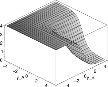
Figure 3: Graph of $\bar{N}(4,4)$ for $y_{A}$ and $y_{B}$ in the range $[-5,5]$.

Clearly, this graph is symmetric with respect to $y_{A}$ and $y_{B}$.

Let us now also consider, for this same example, the graph of the average number of particles of kind $A$, i.e. $\bar{N}_{A}(4,4)$. The expression follows from (6.12). The graph is given in Figure 4.

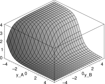
Figure 4: Graph of $\bar{N}_{A}(4,4)$ for $y_{A}$ and $y_{B}$ in the range $[-5,5]$.

Comparing Figure 3 with Figure 4, one can make a distinction between four different regions in terms of the energy variables $y_{A}$ and $y_{B}$. The sector $(y_{A}<0,y_{B}>0)$ is populated mostly with particles of kind $A$, and the sector $(y_{A}>0,y_{B}<0)$ mostly with particles of kind $B$. In the sector $(y_{A}<0,y_{B}<0)$, the population of particles of kind $A$ and of kind $B$ is approximately the same. Finally, the sector $(y_{A}>0,y_{B}>0)$ is essentially unpopulated. The average number of accommodated particles is never bigger that 4, as it should be, since $p=4$.

7 Concluding remarks

In the present paper we have studied the thermal properties of “free” particles, which interact only via statistical interaction. The latter stems from the restrictions imposed by the Pauli principle : the system under consideration cannot accommodate more that $p$ particles if the order of statistics is $p$. This property holds independently of the number of orbitals; there can even be infinitely many.

By definition $A$-statistics is closely related to certain (more precisely, symmetric or Fock) representations of the Lie algebra $sl(n+1)$, including $n=\infty$. Apart from that, $A$-statistics belongs to the class of exclusion statistics as defined in [28, Section 5]. Okubo [29] has also reformulated this in the language of Lie-triple systems. In [16] we have argued that under certain natural assumptions $A$-statistics can be interpreted as an exclusion statistics in the sense of Wu [7].

Apart from the general case we have considered some specific examples. In particular we have shown that for $n=1$ and any $p$ the FD distribution function ($n=1$, $p=1$) deforms into the BE distribution function ($n=1$, $p=\infty$) with the growth of $p$, see Figure 1. In this case $A$-statistics reduces to Gentile statistics [1] (see also [30]). In the more general case of any number of orbitals $n$ the above picture is modified. In the limit $p\rightarrow\infty$ one obtains again the Bose distribution function ${\bar{N}}(p=\infty,n)=nx/(1-x)$. However at $p=1$ the distribution function ${\bar{N}}(p=1,n)$ is a distribution function of hard-core fermions, see (4.29), and not of fermions.

Another observation to mention is in the case with equidistant energy levels. Without any input from quantum groups it turns out that the GPF is a $q$-deformation of the GPF of the most degenerate case. More precisely, the equidistant GPF (5.8) is obtained from the “nondeformed” GPF (4.4) by a $q$-deformation of the binomial coefficients. Another property natural to expect, demonstrated here for $p=1$, is that at very low temperatures the average number of particles of the system is the same as the average number of particles on the lowest energy level, which means that all allowed particles (in the general case $p$) “condensate” on the lowest level.

Despite of the fact that $A$-statistics does not belong to the class of deformed Bose statistics, it yields a good approximation to Bose statistics. Apart from that the Fock spaces do not contain states with negative norm. Therefore, parallel to quons, $A$-statistics with large values of $p$ is a good candidate for the description of small violations of Bose statistics in quantum field theory. Similarly as for quons [24] however, we do not know how to satisfy the locality condition in relativistic quantum field theory. Therefore, one cannot expect to derive relations between charge conjugation, unitarity and statistics as in [31]. It would be interesting to see whether such relations can be derived in the frame of causal $A$-statistics [32].

Finally we point out that our considerations are incomplete in the sense of traditional thermodynamics, because we have not introduced the concept of volume and hence of pressure, etc. In our picture the volume can be introduced in several ways. One natural way would be to relate the order of statistics $p$ to a unit volume $V$ : if $p$ is the maximal number of particles to be accommodated in $V$, then it is natural to assume that twice more particles could be accommodated in the volume $2V$. This is one, but not the only plausible possibility. We shall return to this issue elsewhere.

Appendix : Proof of equation (5.13)

First, we wish to find an expression for $h_{k}(x_{1},\ldots,\hat{x}_{i},\ldots,x_{n})$. The notation $\hat{x}_{i}$ means that $x_{i}$ has been removed from the list of variables $(x_{1},\ldots,x_{n})$, so $h_{k}(x_{1},\ldots,\hat{x}_{i},\ldots,x_{n})$ stands for a symmetric function in $n-1$ variables. Multiplying (3.7) by $(1-x_{i}t)$, it follows easily that

$$h_{k}(x_{1},\ldots,\hat{x}_{i},\ldots,x_{n})=h_{k}({\bf x})-x_{i}h_{k-1}({\bf x}),$$

where $h_{k}({\bf x})\equiv h_{k}(x_{1},x_{2},\ldots,x_{n})$.

Consider now the general expression for $\bar{l}_{i}$, as given in (3.19) :

$$\bar{l}_{i}={1\over Z(p,n)}x_{i}\partial_{x_{i}}Z(p,n),$$

or, using (3.4),

$$x_{i}\partial_{x_{i}}Z(p,n) = \sum_{0\leq l_{1}+l_{2}+\cdots+l_{n}\leq p}l_{i}x_{1}^{l_{1}}x_{2}^{l_{2}}\cdots x_{n}^{l_{n}}$$

$$= \sum_{l_{i}=0}^{p}l_{i}x_{i}^{l_{i}}\sum_{0\leq l_{1}+\cdots+l_{i-1}+l_{i+1}+\cdots+l_{n}\leq p}x_{1}^{l_{1}}\cdots x_{i-1}^{l_{i-1}}x_{i+1}^{l_{i+1}}\cdots x_{n}^{l_{n}}$$

$$= \sum_{l_{i}=0}^{p}l_{i}x_{i}^{l_{i}}\sum_{k=0}^{p-l_{i}}\sum_{(l_{1}+\cdots+l_{i-1}+l_{i+1}+\cdots+l_{n}=p-k)}x_{1}^{l_{1}}\cdots x_{i-1}^{l_{i-1}}x_{i+1}^{l_{i+1}}\cdots x_{n}^{l_{n}}$$

$$= \sum_{l_{i}=0}^{p}l_{i}x_{i}^{l_{i}}\sum_{k=0}^{p-l_{i}}h_{k}(x_{1},\ldots,\hat{x}_{i},\ldots,x_{n})$$

$$= \sum_{l_{i}=0}^{p}l_{i}x_{i}^{l_{i}}\sum_{k=0}^{p-l_{i}}(h_{k}({\bf x})-x_{i}h_{k-1}({\bf x})).$$

In this last expression, we can make the specialization $x_{i}=q^{i-1}x$. From (5.7) we know already how the functions $h_{k}({\bf x})$ specialize, so there comes (replacing also the summation variable $l_{i}$ by $l$)

$$\sum_{l=0}^{p}l(q^{i-1}x)^{l}\sum_{k=0}^{p-l}\left(\left[n+k-1\atop k\right]x^{k}-q^{i-1}x\left[n+k-2\atop k-1\right]x^{k-1}\right).$$

Replacing $q^{i-1}$ by a new variable $\alpha$, this can be rewritten as

$$\sum_{l=0}^{p}\sum_{k=0}^{p-l}l\alpha^{l}\left(\left[n+k-1\atop k\right]-\alpha\left[n+k-2\atop k-1\right]\right)x^{k+l}.$$

Collecting equal powers of $\alpha$, this reduces to

$$\sum_{l=1}^{p}\alpha^{l}\sum_{k=0}^{p-l}\left[n+k-1\atop k\right]x^{k+l}.$$ (A.1)

Putting back $\alpha=q^{i-1}$ gives the relation (3.69), which we wanted to prove.

Observe that one summation can be performed in (A.1) :

$$\sum_{l=1}^{p}\alpha^{l}\sum_{k=0}^{p-l}\left[n+k-1\atop k\right]x^{k+l} = \sum_{k=0}^{p-1}\left[n+k-1\atop k\right]x^{k}\sum_{l=1}^{p-k}(\alpha x)^{l}$$

$$= \sum_{k=0}^{p-1}\left[n+k-1\atop k\right]x^{k}\bigl{(}{\alpha x-(\alpha x)^{p-k+1}\over 1-\alpha x}\bigr{)}.$$

Replacing again $\alpha$ by $q^{i-1}$ yields an alternative expression for (5.13).