String Theory and Hybrid Inflation/Acceleration

Abstract:

We find a description of hybrid inflation in (3+1)-dimensions using brane dynamics of Hanany-Witten type. P-term inflation/acceleration of the universe with the hybrid potential has a slow-roll de Sitter stage and a waterfall stage which leads towards an $\mathcal{N}=2$ supersymmetric ground state. We identify the slow-roll stage of inflation with a non-supersymmetric ‘Coulomb phase’ with Fayet-Iliopoulos term. This stage ends when the mass squared of one of the scalars in the hypermultiplet becomes negative. At that moment the brane system starts undergoing a phase transition via tachyon condensation to a fully Higgsed supersymmetric vacuum which is the absolute ground state of P-term inflation. A string theory/cosmology dictionary is provided, which leads to constraints on parameters of the brane construction from cosmological experiments. We display a splitting of mass levels reminiscent of the Zeeman effect due to spontaneous supersymmetry breaking.

1 Introduction

Recently it was pointed out in [1] that the Salam-Strathdee-Fayet $\mathcal{N}=2$ SUSY gauge model [2] provides a new type of inflationary model. The theory has a $U(1)$ vector multiplet, a charged hypermultiplet and a Fayet-Iliopoulos (FI) term. In hypersymmetry ($\mathcal{N}=2$ supersymmetry) one has a triplet of prepotentials, $P^{r}$. They may have some constant values $P^{r}=\xi^{r}$ that correspond to FI terms in $\mathcal{N}$=2 supersymmetry. The cosmological theory based on this model was called in [1] ‘hybrid hypersymmetric model,’ or P-term inflation, since the scalar potential of this model corresponds to a hybrid-type potential [3] with P-term.

P-term inflation is related to D-term inflation theory [4], for the case when the gauge coupling $g$ is related to the Yukawa coupling $\lambda$ by $\lambda^{2}=2g^{2}$. The potential also coincides with the F-term inflationary potential studied in [5, 6]. Such models are considered to be semi-realistic models of inflation in the early universe (see for example [6, 7, 8]). A nice introductory account of the early universe acceleration (the cosmological inflation) and the present epoch acceleration can be found in [9]. In [1] it has been suggested that P-term inflation with different parameters, gauge coupling and FI terms, may also be used for explaining the acceleration of the universe at the present epoch, with the cosmological constant $\Lambda={\xi}^{2}/2$.

The purpose of this paper is to describe the connection between a brane construction of string theory and the cosmological aspects of the hybrid hypersymmetric model with P-term inflation/acceleration. By making this connection we may constrain parameters of the brane model using the recent cosmological observations [10, 11, 12].

Gauge theories related to brane configurations have been extensively studied in the last few years, based on D-brane technology motivated by the work of Polchinski [13]-[15]. The brane model herein is based on those of Witten [16] and Hanany-Witten [17], which have been thoroughly discussed and extended by Giveon and Kutasov [18]. Specifically, the model involves two parallel $NS5$-branes with a $D4$-brane suspended between them and a $D6$-brane orthogonal to both the $D4$-brane and the $NS5$-branes. Such system preserves $\mathcal{N}=2$ $D=4$ supersymmetry. However, a certain displacement $\Delta L$ of the $NS5$-branes will break supersymmetry spontaneously, as discussed recently by Brodie [19]. This provides positive vacuum energy which, from the cosmological viewpoint, triggers inflation.

We will find that in our brane model one can express the FI term $\xi$ as well as the gauge coupling $g$ of the cosmological model through a combination of the string coupling $g_{s}$, string length $l_{s}$, the distance $L$ between heavy branes, and their displacement $\Delta L$ from the supersymmetric position.

It has been shown [6, 7, 8] that for F and D-term inflation in the early universe with 60 e-foldings, some combination of the parameters of the relevant inflationary models can be defined by the COBE measurement of CMB anisotropy [10] as follows: $\xi/g\sim 10^{-5}M_{P}^{2}$. In our brane model of P-term inflation this yields the relation

$$\left({\Delta L\over 2\pi g_{s}l_{s}}\right)_{\rm COBE}\sim 10^{-5}\left({2\pi l_{s}\over l_{P}}\right)^{2}\ .$$ (1)

Here $l_{P}^{-1}=M_{P}\sim 2.4\times 10^{18}\ GeV$.

Applying the model to the present epoch acceleration we can use the indication from experiments on supernovae [11] and recent CMB observations [12] that the likely value of the cosmological constant is $\Lambda_{present}\sim 10^{-120}M_{P}^{4}$. Using the relation $\Lambda=\xi^{2}/2$, it follows that for the brane model describing today’s acceleration we get

$$\left({(\Delta L)^{2}\over 2g_{s}l_{s}L}\right)_{\rm present}\sim 10^{-120}\left({2\pi l_{s}\over l_{P}}\right)^{4}\ .$$ (2)

We will point out the significance of the $\mathcal{N}=2$ FI terms and show how the Coulomb branch, the mixed Coulomb-Higgs branch, and the fully Higgsed branch of the brane construction are related to the slow-roll de Sitter stage, a waterfall stage, and an absolute $\mathcal{N}=2$ supersymmetric ground state of the hybrid hypersymmetric model of inflation/acceleration in [1]. The connection is made more explicit by matching the masses of the scalars in the hypermultiplet and the one-loop potential computed from the field theory side with the ones computed from open string theory. In the absence of FI term neither our gauge model nor the brane construction lead to any interesting cosmological models. However, when FI terms are present, we find in the gauge theory that the de Sitter type vacuum breaks supersymmetry spontaneously, a fact which is also imprinted in the whole string spectrum through the vanishing of the supertrace. Notice that a spontaneously broken symmetry means that the underlying symmetry may still control the system as it happens for the standard model.

We will establish a relation between Sen’s tachyon condensation in open string theory [20] and tachyon condensation in the context of preheating in hybrid inflation studied by Felder, Garcia-Bellido, Greene, Kofman, Linde and Tkachev [21]. In P-term inflation, when the system passes the bifurcation point, the tachyonic instability develops with the consequent waterfall to the $\mathcal{N}=2$ supersymmetric ground state.

2 The potential of the P-term inflation model

The potential of the hybrid hypersymmetric model [1] is

$$V={g^{2}\over 2}\left[(|\Phi_{1}|^{2}+|\Phi_{2}|^{2})|\Phi_{3}|^{2}+|\Phi_{1}|^{2}|\Phi_{2}|^{2}+{1\over 4}\left(|\Phi_{1}|^{2}-|\Phi_{2}|^{2}+\frac{2{\xi}}{g}\right)^{2}\right]\ ,$$ (3)

which is depicted in Figure 1.

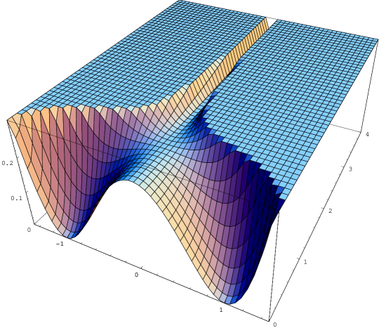
Figure 1: Cosmological potential with Fayet-Iliopoulos term. De Sitter valley is classically flat; it is lifted by the one-loop correction corresponding to the one-loop potential between $D4$-$D6$. In this figure the valley is along the $|\Phi_{3}|$ axis; the orthogonal direction is a line passing through the origin of the complex $\Phi_{2}$ plane and we have put $|\Phi_{1}|=0$. Notice there is no $\mathbb{Z}_{2}$ symmetry of the ground state, it is just a cross section of the full $U(1)$ symmetry corresponding to the phase of the complex $\Phi_{2}$ field. The fields are shown in units of $\sqrt{\xi/g}$. The bifurcation point corresponds to $|\Phi_{3}|=\sqrt{\xi/g}$, $\Phi_{2}=0$. The absolute minimum is at $\Phi_{3}=0$, $\Phi_{2}=\sqrt{2\xi/g}$.

Here $\Phi_{3}\equiv A+iB$ is a complex scalar from the $\mathcal{N}=2$ vector multiplet and the two complex scalars $\Phi_{1}\equiv a_{1}+ib_{1}$ and $\Phi_{2}\equiv a_{2}+ib_{2}$ form a quaternion of the hypermultiplet, charged under the $U(1)$ group. The FI P-term here is $\vec{\xi}=(0,0,\xi)$. All 6 real scalars $\phi_{i}=\{A,B,a_{1},b_{1},a_{2},b_{2}\}$ have canonically normalized kinetic terms in the Lagrangian of the form

$$L_{\rm kin}={1\over 2}\sum_{i=1}^{i=6}(\partial\phi_{i})^{2}={1\over 2}|\partial\Phi_{1}|^{2}+{1\over 2}|\partial\Phi_{2}|^{2}+{1\over 2}|\partial\Phi_{3}|^{2}.$$ (4)

The potential (3) has a local minimum, corresponding to a de Sitter space when coupled to gravity, with $|\Phi_{3}|$ being a flat direction. These classical vacua break all the supersymmetry spontaneously; here, the vev of the hypers vanishes, $\langle\Phi_{1}\rangle=\langle\Phi_{2}\rangle=0$, and the vev of the scalar from the vector multiplet, which is the inflaton field, is non-vanishing, $\langle\Phi_{3}\rangle\neq 0$. The masses of all the fields in the de Sitter valley are as follows: in the vector multiplet the gauge field $A_{\mu}$ and a gaugino $\lambda_{A}$ are massless, whereas the masses of the fields in the hypermultiplet are split:

$$M^{2}_{2}=g^{2}|\Phi_{3}|^{2}-g{\xi}\ ,\qquad M_{\psi}=g|\Phi_{3}|\ ,\qquad M_{1}^{2}=g^{2}|\Phi_{3}|^{2}+g{\xi}\ .$$ (5)

Here $\psi$ is the hyperino, $\Phi_{1}$ ($\Phi_{2}$) are positively (negatively) charged scalars of the hypermultiplet. The value of the potential at this vacuum is $V={\xi}^{2}/2$. This is the cosmological constant driving the exponential expansion of the universe. This state corresponds to a Coulomb branch of the $\mathcal{N}=2$ gauge theory. The presence of the FI term breaks supersymmetry spontaneously, which is imprinted in the fact that the supertrace of the mass spectrum vanishes [22]

$$\mbox{STr}\,M^{2}\equiv\sum_{j}(-1)^{2j}(1+2j)M_{j}^{2}=0,$$ (6)

where $j$ is the spin of the state. The right hand side of this equation vanishes in our case since the total $U(1)$ charge vanishes for the hypermultiplet.

The point where one of the scalars in the hypermultiplet becomes massless,

$$M^{2}_{2}=g^{2}|\Phi_{3}|_{c}^{2}-g{\xi}=0\ \ \Leftrightarrow\ \ |\Phi_{3}|_{c}=\sqrt{\xi\over g}$$ (7)

is a bifurcation point. At $|\Phi_{3}|^{2}\leq{\xi}/g$, the de Sitter minimum becomes a de Sitter maximum; beyond it, such scalars become tachyonic. The system is unstable and the waterfall stage of the potential leads it to a ground state. The waterfall stage has non-vanishing vev’s for the scalars in both the hyper and vector multiplets; this is a mixed Coulomb-Higgs branch. Finally, the system gets to the absolute minimum with vanishing vev for the scalars in the vector multiplet, $\langle\Phi_{3}\rangle=0$, and non-vanishing vev for the scalars in hypermultiplet, $\langle\Phi_{2}\rangle^{2}=2{\xi}/g$. Supersymmetry is unbroken and all fields are massive; they form a massive $\mathcal{N}=2$ vector multiplet with $M^{2}=2g{\xi}$. This is a fully Higgsed branch of the gauge theory.

Since the potential is flat in the $|\Phi_{3}|$ direction, the inflaton field, $\Phi_{3}$, does not naturally move. However, the gauge theory one-loop potential lifts the flat direction, via a logarithmic correction [5, 4, 6, 7, 8]

$$V={1\over 2}{\xi}^{2}+{g^{2}\over 16\pi^{2}}{\xi}^{2}\ln{|\Phi_{3}|^{2}\over|\Phi_{3}|_{c}^{2}}.$$ (8)

This is precisely what is necessary to provide a slow roll-down for the inflaton field, since it is an attractive potential which leads to the motion of the field $\Phi_{3}$ towards the bifurcation point and to the end of inflation. Note that in $\mathcal{N}=2$ supersymmetric gauge models there are no higher loop infinities [23].

Before proceeding to the string theory model for hybrid inflation, we would like to stress that in the absence of FI term $\xi$ none of the interesting things takes place. The potential with $\xi=0$ is plotted in Figure 2. There is a Minkowski valley with the flat direction.

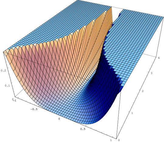
Figure 2: Cosmological potential without Fayet-Iliopoulos term. The motion of the D4 corresponds to moving along the bottom of the valley, which has a zero potential.

3 NS5-D4/D6-NS5 model

We will now discuss one of the possible brane constructions describing hybrid inflation. The picture is based on the one studied in [16]-[19] in (3+1)-dimensions. As a warm up, let us explain the supersymmetric version of this construction, corresponding to the absence of FI terms, which is depicted in Figure 3.

The following table summarizes the brane configuration, where $\times$s indicate directions in which branes are lying.

	0	1	2	3	4	5	6	7	8	9
$D4$	$\times$	$\times$	$\times$	$\times$			$\times$
$D6$	$\times$	$\times$	$\times$	$\times$				$\times$	$\times$	$\times$
$NS5$	$\times$	$\times$	$\times$	$\times$	$\times$	$\times$

This brane model consists of two $NS5$-branes with a $D4$-brane suspended between them. The field theory on the $D4$-brane is effectively (3+1)-dimensional since one of the $D4$-brane worldvolume directions is finite, with length $L$. Thus, Kaluza-Klein modes may be ignored as long as we are probing energies smaller than $1/L$, and physics is effectively (3+1)-dimensional in the worldvolume theory. The $NS5$-branes play still another role. They freeze the motion of the $D4$-brane in the $7,8,9$ directions. Hence, such scalars will not appear in the worldvolume theory; the only scalars arising therein correspond to motions in the $4,5$ direction, and form the two real scalars of the $\mathcal{N}=2$ vector multiplet.

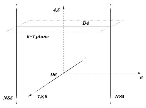
Figure 3: Brane configuration without Fayet-Iliopoulos term. We are free to move D4 in 4,5 directions with no energy cost.

In order to include matter in the $D4$-brane worldvolume theory, we introduce a $D6$-brane. The (4-6) and (6-4) strings will then form an $\mathcal{N}=2$ hypermultiplet. The spectrum of these strings is given with some detail in Appendix A. Moreover, including the $D6$-brane does not break any further supersymmetry, since the projectors of the supersymmetry conditions are compatible with the ones of the $NS5$ and $D4$. Therefore, the worldvolume theory on the $D4$-brane is a (3+1)-dimensional, $\mathcal{N}=2$ $U(1)$ gauge theory with one charged hypermultiplet. Of course this is exactly the theory discussed in section 2 without the FI term. Due to supersymmetry we are free to move the $D4$-brane along the directions $4,5$ at no energy cost. This corresponds to motion along the Minkowski valley in Figure 2 and the Coulomb branch of the gauge theory.

A much more interesting situation takes place when we turn on the Fayet-Iliopoulos term, as emphasized in the last section for cosmological applications. Consider displacing the $NS5$-branes along direction 7 as shown in Figure 4a). Since the $D4$-brane has to remain connected to the $NS5$-branes, this introduces an angle $\phi$ between the $D4$-brane and the $D6$-brane, which in general breaks supersymmetry. As we shall see, this angle $\phi$ corresponds in the field theory language to the FI parameter.

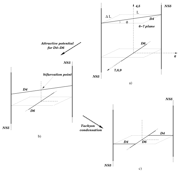
Figure 4: Brane configuration evolution with Fayet-Iliopoulos term. a) For $\phi\neq 0$, supersymmetry is broken and D4-D6 experience an attractive force. b) At the bifurcation point, a complex scalar in the hypermultiplet becomes massless; when we overshoot tachyon instability forms, taking the system to a zero energy ground state shown in c) .

If initially $\phi\neq 0$, the system is unstable. One consequence is the attractive potential driving the $D4$-brane towards the $D6$-brane, with the former sliding down the $NS5$-branes. One might also think that the $D4$-brane tries to minimize the angle with the $D6$-brane, by effectively trying to pull the $NS5$-branes to the origin of direction 7. The latter effect causes the bending of the $NS5$-branes. We do not expect such an effect to drive the system towards a supersymmetric and hence minimal energy configuration, since the $NS5$-branes will be bent. In particular it cannot bring the configuration back to the supersymmetric system in Figure 3. Of course the effect can be always negligible if we consider large $NS5$-brane tension corresponding to weak string coupling.

The most important dynamical effect is therefore the attractive potential between $D4$ and $D6$. We will show below that the open string theory one-loop potential matches exactly (8), which is derived from field theory. Therefore the motion of the $D4$ towards the $D6$ is the slow roll down of the inflaton. Hence it is a Coulomb branch with vanishing vev’s for the scalars in the hypermultiplet and non-vanishing vev’s for scalars in the vector multiplet.

To make the connection with the Coulomb phase more concrete at this stage we use the spectrum of 6-4 and 4-6 open strings in the presence of the angle $\phi$. We can see from Figure 4 that the boundary conditions are slightly unusual in the 6-7 plane. In terms of $Z=X^{6}+iX^{7}$ and the rotation angle $\phi$ we require:

$$\sigma_{1} = 0\quad(D4)\qquad\partial_{\sigma_{1}}\rm{Re}\left(e^{i\phi}Z\right)=\rm{Im}\left(e^{i\phi}Z\right)=0,$$

$$\sigma_{1} = \pi\quad(D6)\qquad\partial_{\sigma_{1}}\rm{Im}\ Z=\rm{Re}\ Z=0,$$ (9)

For $\phi=0$, these reduce to ordinary Dirichlet-Neumann (DN) boundary conditions. The calculation of the spectrum of low lying states of the open strings exactly reproduces the split in the hypermultiplet masses shown in eq. (5). By comparing these two spectra we will identify the dictionary between the parameters of the brane construction and cosmology.

4 String theory–cosmology dictionary

The relevant part of the string spectrum obtained in Appendix A gives

$$M^{2}_{\pm}={g_{{}_{YM}}^{2}(\widetilde{\Delta s})^{2}\over l_{s}^{4}}\pm{g_{{}_{YM}}\tilde{\phi}\over 2\pi l_{s}^{2}}\ ,\qquad M_{\psi}^{2}={g_{{}_{YM}}^{2}(\widetilde{\Delta s})^{2}\over l_{s}^{4}}\ ,$$ (10)

$$(\widetilde{\Delta s})^{2}\equiv{(x^{4})^{2}+(x^{5})^{2}\over g_{{}_{YM}}^{2}{\pi^{2}}}\ .$$ (11)

Notice that despite the fact that the gauge theory is abelian, we use the Yang-Mills subscript $g_{{}_{YM}}$, as a reminder that it is a gauge coupling of the fields on the brane. We define the string length as $\alpha^{\prime}=l_{s}^{2}$. Since the kinetic terms on the field theory side are canonically normalized, we had to redefine the fields from the open string theory side such that

$$\Delta s=g_{{}_{YM}}(\widetilde{\Delta s}),\ \ \ \ \phi=g_{{}_{YM}}\tilde{\phi}.$$ (12)

For the Fayet-Iliopoulos parameter we use the convention of [2], for which the cosmological constant depends solely on the FI parameter (not on the coupling). In this fashion the fields in the $D$-brane action, which has initially in front a $1/g_{s}$ factor, will get the same canonical normalization. Using the conventions of Polchinski [14] and taking into account the compact dimension, the relation between couplings is

$$g_{{}_{YM}}^{2}=(2\pi)^{2}g_{s}{l_{s}\over L}.$$ (13)

Comparison between formulae (5) and (10) yields the dictionary between field theory parameters (left) and string theory parameters (right)

$$g \longleftrightarrow g_{{}_{YM}}=2\pi\sqrt{g_{s}\frac{l_{s}}{L}},$$

$$|\Phi_{3}| \longleftrightarrow \frac{\widetilde{\Delta s}}{l_{s}^{2}},$$ (14)

$${\xi} \longleftrightarrow \frac{\tilde{\phi}}{2\pi l_{s}^{2}}.$$

For small angles $L\phi=L\sin\phi$, which is the distance in direction 7 between the NS5 branes after they have been pulled out. We will therefore use the notation $L\phi\equiv\Delta L$. The FI term is related to the string construction by a simple formula which in string units simply states that it is a ratio between the pull out distance and the finite size of the $D4$-brane

$${\xi}={\Delta L\over L}{1\over 2\pi l_{s}^{2}}{1\over g_{{}_{YM}}}.$$ (15)

As we have explained in the beginning of the paper, a combination of the FI term $\xi$ and gauge coupling $g$ is constrained by recent cosmological observations and it is very nice to find out a possible interpretation of these important parameters in string theory.

5 Spontaneous supersymmetry breaking, potential and tachyon condensation

In field theory, spontaneous breaking of supersymmetry manifests itself through the vanishing of the supertrace, as in equation (6). We have seen this to be the case in the field theory description of the Coulomb phase, corresponding in the cosmological picture to the slow-roll period of inflation. Of course, the field theory contains only the low lying states of the string theory. So it is natural to ask if the supertrace vanishes for the whole tower of string states in the $D4$-$D6$ system with an angle. To check this, we only need the partition function, $\mathcal{Z}=\mathcal{Z}(q)$, which is shown in appendix B. Then, the supertrace can be expressed as

$$\mbox{STr}M^{2}=\left.{2\over\alpha^{\prime}}q{\partial\over\partial q}\mathcal{Z}\right|_{q=1}.$$ (16)

An explicit calculation shows that the supertrace is indeed vanishing. In fact, we find it rather impressive that there is a mass splitting such that the supertrace vanishes at each level. We illustrate such ‘stringy Zeeman effect’ in figure 5. This indicates that supersymmetry is spontaneously broken in the full string theory.

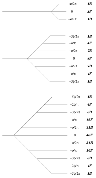
Figure 5: Splitting of mass for the first three levels due to the presence of an angle $\phi$. Notice that at each level the supertrace vanishes. On the right we show the number of bosonic (B) or fermionic (F) states with such mass for either the 4-6 or 6-4 strings. The total number of states is twice as many.

We may now proceed to Figure 4b). In gauge theory, the one-loop quantum correction (8) to the classical potential, drives the inflaton towards the bifurcation point at $|\Phi_{3}|^{2}=\xi/g$. The open string one-loop potential is expected to provide an analogous attractive potential between the $D4$ and $D6$-branes. The one-loop vacuum amplitude corresponding to the effective interaction between $D4$ and $D6$-branes is given by

$$V = -\frac{2}{2}\int_{0}^{\infty}{dt\over t}\int_{-\infty}^{\infty}\frac{d^{4}p}{(2\pi)^{4}}\left[\mbox{Tr}_{NS}{1+(-1)^{F}\over 2}e^{-2\pi tL_{0}^{NS}}-\mbox{Tr}_{R}{1+(-1)^{F}\over 2}e^{-2\pi tL_{0}^{R}}\right].$$ (17)

The operator ${1\over 2}(1+(-1)^{F})$ is the GSO projection. The factor of $2$ in the coefficient is due to the contribution of both 4-6 and 6-4 strings. Some details of the calculation can be found in appendix C. The result is

$$V = \left({1\over 8\pi^{2}\alpha^{\prime}}\right)^{2}{\sin^{2}\phi\over\cos\phi}\int_{\alpha^{\prime}/\Lambda^{2}}^{\infty}{dt\over t}\exp\left[-2\pi t{(\Delta s)^{2}\over\alpha^{\prime}}\right]+{\cal O}(e^{-\pi/t}),$$ (18)

$$\sim {g_{{}_{YM}}^{2}\over 16\pi^{2}}\left(\frac{\tilde{\phi}}{2\pi\alpha^{\prime}}\right)^{2}\log{(\Delta s)^{2}\over\Lambda^{2}}.$$

This exactly reproduces the one-loop correction in the field theory (8), including the numerical coefficient, in the small angle and large separation approximation. Notice that the logarithmic dependence is expected. In fact, the $D6$ and $D4$ branes have two common transverse directions. Since at large separation the dominant contribution comes from the massless closed string exchange, we expect to be dealing with a harmonic potential in two-dimensions. Notice also that the logarithmic divergence we have regularized with the cutoff $\Lambda$ corresponds, from the viewpoint of closed string theory, to an infrared divergence. In the open string channel it is an ultraviolet divergence and originates from the highly massive open string modes, rather than the low lying states that contribute to the one-loop field theory correction. Therefore, it is non-trivial that we obtain a precise matching with the one-loop field theory potential. Similar phenomena have been found in [25], [26].

The potential is attractive and drives the motion of the $D4$ brane towards the $D6$-brane. At a separation defined by the vanishing of the mass of the lowest lying state

$$(\Delta s)^{2}_{B}={\phi\over 2\pi}l_{s}^{2},\$$ (19)

there is a bifurcation point; beyond it, such state becomes tachyonic. Naturally, if the inflaton field gets to the bifurcation point with non-zero velocity, it will overshoot, and the tachyon instability will develop. This is in precise correspondence with the motion on the ridge of the potential in Figure 1 after the bifurcation point, since the de Sitter valley becomes a hill top there, hence an unstable maximum. The actual behaviour of perturbations in such potentials has been investigated numerically in [21] where the tachyonic instability was studied in the context of preheating of the universe after inflation.

Naively, one might expect the fields $\Phi_{2}$ and $\Phi_{3}$ to roll down from the bifurcation point and then experience a long stage of oscillations with amplitude $O(\sqrt{\xi/g})$ near the minimum of the effective potential at $|\Phi_{2}|=\sqrt{2\xi/g}$ until they give their energy to particles produced during these oscillations. However, it was recently found in [21] that the tachyonic instability rapidly converts most of the potential energy $\xi^{2}/2$ into the energy of colliding classical waves of the scalar fields. This conversion, which was called “tachyonic preheating,” is so efficient that symmetry breaking (tachyon condensation) is typically completed within a single oscillation of the field distribution as it rolls towards the minimum of its effective potential.

It is interesting to clarify the connection between such tachyonic instabilities in models of hybrid cosmology and the phenomenon of tachyon condensation in open string theory first discussed by Sen [20]. Typically, the attention in the latter studies was towards brane/antibrane systems with the consequent brane/antibrane annihilation with the tachyon potential being conjectured to cancel completely the brane’s tensions (note that an antibrane is a brane rotated by $\pi$ relative to the first one; the supersymmetric configuration requires the same type of branes to be parallel).

In fact, interesting brane inflation models have been suggested in the framework of brane/antibrane configurations [24]. In this framework tachyon instability develops at brane/antibrane separations of the order of $l_{s}$, with the consequent tachyon condensation. It is suggested therein that such inflation may be of the hybrid inflation type, which is exactly coming out in our study.

The tachyonic instability of our system has also been considered in the context of tachyon condensation in open string field theory [27]. Therein, the system considered is $D0$-$D4$, which is just T-dual to our orthogonal $D4$-$D6$. Moreover, instead of introducing an angle to create the instability, a $B$ field is used. These are just T-dual pictures. When the tachyon develops, it takes the system to a supersymmetric ground state, which is a non-threshold bound state of $D0$ and $D4$-branes. This mass deficit, is precisely the height of our de Sitter valley in Figure 1. The perturbative string theory techniques do not allow us to trace the evolution of the system once the tachyonic instability develops, corresponding to the waterfall stage in the cosmological picture. However, using the open string field theory techniques of [27] one might be able to trace down quantitatively such evolution.

In our case, we know from the cosmological part of our construction that after the bifurcation point the waterfall stage (tachyon condensation) takes place. Instead of continuing at the ridge (in Coulomb phase) the brane system undergoes a phase transition. The system reconfigures itself as to reach the supersymmetric configuration represented in Figure 4c). This is the only supersymmetric configuration possible if we allow only the $D4$-branes to move. It is an $\mathcal{N}=2$ supersymmetric, fully Higgsed phase of the field theory. All fields are massive. This absolute ground state is in precise agreement with the Minkowski ground state of the hybrid potential in Figure 1. Notice that this final configuration, where branes reconnect, is very different from the brane/antibrane scenarios where the branes annihilate after tachyon condensation.

6 Discussion

There are well known problems in incorporating de Sitter space and cosmology into the framework of M/String theory; see the most recent discussions in [28, 29, 30]. In this paper we have described hybrid P-term inflation through a brane construction of string theory. It suggests a path to link string theory and cosmology. One may expect that eventually this direction will be useful in addressing the problems of cosmology where general relativity and gauge theory break down and quantum gravity regime takes place. Here, we only gave a few steps towards realizing a scenario of cosmological inflation/acceleration in string theory. Including gravity is, of course, the main challenge, since at present it is not known how to embed our hybrid hypersymmetric model into $\mathcal{N}=2$ supergravity; only the coupling to $\mathcal{N}=1$ supergravity is known [1].

To include four dimensional gravity in our model we have to resort to compactification, since no promising suggestions on how to localize gravity on $D$-branes have been put forward. But string compactifications of models with branes are very constrained. Physically the flux of the branes in a compact space has to be cancelled. A known example of a consistent string compactification with $D5$ and $D9$-branes was worked out by Gimon and Polchinski [31]. Such models yield $\mathcal{N}=1$ string vacua in six dimensions, containing not only gravity but also the vector and hyper multiplets of the field theory described in this paper, which have a natural origin as $\mathcal{N}=1$ multiplets in six dimensions.

We would like to emphasize again the important role of the Fayet-Iliopoulos term in getting interesting cosmology. In our model it has a simple geometric interpretation, as a displacement of the $NS5$-branes. If we would pursue the suggestion of the previous paragraph, we would have to understand how the FI term arises there. It is known, that it has a geometric interpretation as controlling the resolution of singularities in ALE spaces [32]. A compact version of such spaces is $T^{4}/{\mathbb{Z}}_{2}$. This is an orbifold limit of $K3$, which is precisely the compactification manifold used in [31]. In fact these two interpretations of the FI terms are not unrelated, since it has been argued that under certain circumstances the existence of $NS5$-branes is T-dual to singularities of ALE spaces [33]. It is amusing to think that, in this picture, one could argue for the existence of a positive cosmological constant by requiring smoothness of the ten dimensional space of string theory. Thus, it seems important to understand the coupling of our $\mathcal{N}=2$ gauge theory to $\mathcal{N}=2$ supergravity and to find its string theory interpretation.

Appendix A D4-D6 system with angle

In order to address an audience of non string theory experts, we will give some details of the computation of the string spectrum in this appendix.

We consider the system of $D4$ and $D6$-brane at an angle and separated by some distance. The configuration is as in Figure 4a). We introduce a spacetime complex coordinate $Z=X^{6}+iX^{7}$. The boundary conditions of several types of open strings are summarized in the following table. We will denote Neumann and Dirichlet boundary conditions by N and D respectively.

	$X^{0,1,2,3}$	$X^{4,5}$	$\mbox{Re}Z$	$\mbox{Im}Z$	$\mbox{Re}(e^{i\phi}Z)$	$\mbox{Im}(e^{i\phi}Z)$	$X^{8,9}$
4-4	NN	DD	- -	- -	NN	DD	DD
6-6	NN	DD	DD	NN	- -	- -	NN
4-6	NN	DD	-D	-N	N-	D-	DN
6-4	NN	DD	D-	N-	-N	-D	ND

We parametrize the open string worldsheet by $w=\sigma_{1}+i\sigma_{2}$ with $0\leq\sigma_{1}\leq\pi$ and $-\infty\leq\sigma_{2}\leq+\infty$. The presence of the angle $\phi$ is reflected in the spectrum of the 4-6 and 6-4 strings. The boundary conditions for 4-6 string in $(6,7)$-plane are somewhat unusual and are given in eq. (9), while those in the rest of eight directions satisfy standard NN, DD or DN conditions. Given these boundary conditions, the solution to the equation of motion, $\partial_{w}\partial_{\bar{w}}X^{\mu}=0\quad(\mu=0,1,\cdots,9)$, yields the following expansion for 4-6 string.

($0,1,2,3$)-directions (ordinary NN)

$$X^{i}(w,\bar{w})=x^{i}-2i\alpha^{\prime}p^{i}\sigma_{2}+i\sqrt{{\alpha^{\prime}\over 2}}\sum_{m\in Z\backslash\{0\}}{\alpha_{m}^{i}\over m}\left(e^{imw}+e^{-im\bar{w}}\right),$$ (20)

($4,5$)-directions (ordinary DD)

$$X^{4,5}(w,\bar{w})={x^{4,5}\over\pi}\sigma_{1}+i\sqrt{{\alpha^{\prime}\over 2}}\sum_{m\in Z\backslash\{0\}}{\alpha_{m}^{4,5}\over m}\left(e^{imw}-e^{-im\bar{w}}\right),$$ (21)

($6,7$)-directions (rotated ND and DN)

$$Z(w,\bar{w}) = i\sqrt{{\alpha^{\prime}\over 2}}e^{-i\phi}\left[\sum_{r\in Z+{1\over 2}+{\phi\over\pi}}{1\over r}\alpha_{r}e^{irw}+\sum_{r\in Z+{1\over 2}-{\phi\over\pi}}\bar{\alpha}_{r}e^{-im\bar{w}}\right],$$ (22)

$$\bar{Z}(w,\bar{w}) = i\sqrt{{\alpha^{\prime}\over 2}}e^{+i\phi}\left[\sum_{r\in Z+{1\over 2}-{\phi\over\pi}}{1\over r}\bar{\alpha}_{r}e^{irw}+\sum_{r\in Z+{1\over 2}+{\phi\over\pi}}\alpha_{r}e^{-im\bar{w}}\right],$$ (23)

where $\alpha_{r}$ and $\bar{\alpha}_{r}$ are linearly independent, and their hermitian conjugates satisfy $\alpha^{\dagger}_{r}=-\alpha_{r}$ and $\bar{\alpha}^{\dagger}_{r}=-\bar{\alpha}_{r}$.

($8,9$)-directions (ordinary DD)

$$X^{8,9}(w,\bar{w})=i\sqrt{{\alpha^{\prime}\over 2}}\sum_{m\in Z+{1\over 2}}{\alpha_{m}^{8,9}\over m}\left(e^{imw}-e^{-im\bar{w}}\right).$$ (24)

The mode expansions for fermions $\psi^{\mu}\,(\mu=0,1,\cdots,9)$ are similar. In the NS sector, the modes are shifted by ${1\over 2}$ from those of bosons $X^{\mu}$, while they are the same in the R sector. It is convenient to introduce a complex fermion $\psi=\psi^{6}+i\psi^{7}$, as we have done for bosons. Then we have, for instance, in the NS sector,

$$\psi(w,\bar{w}) = e^{+i\phi}\left[\sum_{r\in Z+{\phi\over\pi}}i^{-1/2}\psi_{r}e^{irw}+\sum_{r\in Z-{\phi\over\pi}}i^{1/2}\bar{\psi}_{r}e^{-ir\bar{w}}\right],$$ (25)

$$\bar{\psi}(w,\bar{w}) = e^{-i\phi}\left[\sum_{r\in Z-{\phi\over\pi}}i^{-1/2}\bar{\psi}_{r}e^{irw}+\sum_{r\in Z+{\phi\over\pi}}i^{1/2}\widetilde{\bar{\psi}}_{r}e^{-ir\bar{w}}\right],$$ (26)

and in the R sector, the modes are shifted by ${1\over 2}$. Now the mass-shell condition is given by $L_{0}=0$ and one can easily find

$$L_{0}^{NS}=N_{B}+N_{F}^{NS}-\alpha^{\prime}M^{2}+{(\Delta s)^{2}\over\alpha^{\prime}}-{\phi\over 2\pi},$$ (27)

for the NS sector, and

$$L_{0}^{R}=N_{B}+N_{F}^{R}-\alpha^{\prime}M^{2}+{(\Delta s)^{2}\over\alpha^{\prime}},$$ (28)

for the R sector. We have defined

$$(\Delta s)^{2}={(x^{4})^{2}+(x^{5})^{2}\over\pi^{2}}.$$ (29)

It is now easy to read off the low lying states of open strings. Taking into account the GSO projection, the lowest mass state turns out to be the NS ground state $|p^{i};s_{3}=-1/2,s_{4}=-1/2\rangle$ (where $p^{i}$ is 4-dimensional momentum) with mass

$$M^{2}_{-}={(\Delta s)^{2}\over(\alpha^{\prime})^{2}}-{\phi\over 2\pi\alpha^{\prime}},$$ (30)

corresponding to two real scalars (together with 6-4 string) in the hypermultiplet. Then the next lowest state is built by $\bar{\psi}_{-\phi/\pi}(\psi^{8}_{0}+i\psi^{9}_{0})|p^{i};s_{3}=-1/2,s_{4}=-1/2\rangle=|p^{i};s_{3}=+1/2,s_{4}=+1/2\rangle$ with mass

$$M^{2}_{+}={(\Delta s)^{2}\over(\alpha^{\prime})^{2}}+{\phi\over 2\pi\alpha^{\prime}},$$ (31)

giving the remaining half of scalars in the hypermultiplet. The spacetime fermions in the hypermultiplet turns out to be the R ground state $|p^{i};s_{1},s_{2}\rangle$ with $s_{1}s_{2}=-1/4$ by the GSO projection, whose mass is

$$M^{2}_{\psi}={(\Delta s)^{2}\over(\alpha^{\prime})^{2}}\ ,$$ (32)

corresponding to two 4-dimensional Weyl spinors (together with 6-4 string).

It is straightforward to carry out the computation of the spectrum for 4-4 and 6-6 strings. So we will not repeat the analysis in these cases, but the massless spectra amount to the dimensional reductions of an ${\cal N}=1$ vector multiplet in 10-dimensions down to 5- and 7-dimensions respectively. In our case we are only interested in the gauge theory of the $D4$-brane suspended between two $NS5$-branes, so 6-6 strings decouple from the dynamics and also the collective excitations of the $D4$-brane given by 4-4 strings in 6,7,8 and 9 directions are frozen due to the suspension of the $D4$-brane between two $NS5$-branes. Thus the massless spectrum of 4-4 strings reduces to an ${\cal N}=2$ vector multiplet in 4-dimensions.

Appendix B The Supertrace of $M^{2}$

In order to compute the supertrace (6) we need the partition function. The partition function for the bosonic part is evaluated as

$$\mathcal{Z}_{B}=\mbox{Tr}e^{-2\pi t\left(N_{B}+N_{bc}\right)} = \prod_{m=1}^{\infty}(1-q^{m})^{-4}(1-q^{m-1/2-\phi/\pi})^{-1}(1-q^{m-1/2+\phi/\pi})^{-1}$$ (33)

$$\times(1-q^{m-1/2})^{-2},$$

where we introduced $q=e^{-2\pi t}$. In this expression, $N_{bc}$ is the number operator for the ghosts. Similarly we will introduce $N_{\beta\gamma}^{NS}$ and $N_{\beta\gamma}^{R}$. The partition function for the fermionic part is computed as

$$\mathcal{Z}_{NS}=\mbox{Tr}_{NS}{1+(-1)^{F}\over 2}e^{-2\pi t\left(N_{F}^{NS}+N_{\beta\gamma}^{NS}\right)} = {1\over 2}\cdot 2\prod_{m=1}^{\infty}(1+q^{m-1/2})^{4}(1+q^{m})^{2}$$ (34)

$$\times(1+q^{m-\phi/\pi})(1+q^{m-1+\phi/\pi})$$

in the NS sector, and

$$\mathcal{Z}_{R}=\mbox{Tr}_{R}{1+(-1)^{F}\over 2}e^{-2\pi t\left(N_{F}^{R}+N_{\beta\gamma}^{R}\right)} = {1\over 2}\cdot 4\prod_{m=1}^{\infty}(1+q^{m})^{4}(1+q^{m-1/2})^{2}$$ (35)

$$\times(1+q^{m-1/2-\phi/\pi})(1+q^{m-1/2+\phi/\pi})$$

in the R sector. The full partition function for either the 4-6 or 6-4 strings therefore amounts to

$$\mathcal{Z} = q^{(\Delta s)^{2}/\alpha^{\prime}}\prod_{m=1}^{\infty}(1-q^{m})^{-4}(1-q^{m-1/2-\phi/\pi})^{-1}(1-q^{m-1/2+\phi/\pi})^{-1}(1-q^{m-1/2})^{-2}$$ (36)

$$\times \left[q^{-\phi/(2\pi)}\prod_{m=1}^{\infty}(1+q^{m-1/2})^{4}(1+q^{m-\phi/\pi})(1+q^{m-1+\phi/\pi})(1+q^{m})^{2}\right.$$

$$\left.-2\prod_{m=1}^{\infty}(1+q^{m})^{4}(1+q^{m-1/2-\phi/\pi})(1+q^{m-1/2+\phi/\pi})(1+q^{m-1/2})^{2}\right].$$

The supertrace now follows using expression (16). To get the idea why it is so, let us extract the contributions from the low-lying states corresponding to the scalars and the fermions in the hypermultiplet of the gauge theory:

$$\mathcal{Z}_{\mbox{{\scriptsize hyper}}}=q^{(\Delta s)^{2}/\alpha^{\prime}-\phi/(2\pi)}+q^{(\Delta s)^{2}/\alpha^{\prime}+\phi/(2\pi)}-2q^{(\Delta s)^{2}/\alpha^{\prime}}.$$ (37)

Notice that the exponents of $q$ are indeed $\alpha^{\prime}M^{2}$ of the scalars and the fermions. Thus the supertrace formula (16) gives us

$$\left.{2\over\alpha^{\prime}}q{\partial\over\partial q}\mathcal{Z}_{\mbox{{\scriptsize hyper}}}\right|_{q=1}=2\left((\Delta s)^{2}/(\alpha^{\prime})^{2}-\phi/(2\pi\alpha^{\prime})\right)+2\left((\Delta s)^{2}/(\alpha^{\prime})^{2}+\phi/(2\pi\alpha^{\prime})\right)-4(\Delta s)^{2}/(\alpha^{\prime})^{2}.$$ (38)

This is exactly the supertrace of $M^{2}$ for the ${\cal N}=2$ hypermultiplet.

Now it is straightforward to compute the supertrace (16). In terms of $\vartheta$-functions, $\vartheta_{\alpha\beta}(\nu,it)$, and the Dedekind $\eta$-function, $\eta(t)$, the partition function is given by

$$\mathcal{Z} = {1\over 2}e^{-2\pi t(\Delta s)^{2}/\alpha^{\prime}}\eta(t)^{-6}\frac{\vartheta_{10}(0,it)\vartheta_{00}(0,it)}{\vartheta_{01}(\phi t/(i\pi),it)\vartheta_{01}(0,it)}$$ (39)

$$\qquad\times\left[\vartheta_{00}(0,it)\vartheta_{10}(\phi t/(i\pi),it)-\vartheta_{10}(0,it)\vartheta_{00}(\phi t/(i\pi),it)\right].$$

Since we are interested in the behavior of the partition function at small $t$ or equivalently at $q\to 1$, we will use the modular transformations for $\vartheta$-functions:

$$\vartheta_{01}(\phi t/(i\pi),it) = 2\cos\phi e^{t\phi^{2}/\pi-\pi/(4t)}t^{-1/2}\prod_{m=1}^{\infty}(1-e^{-2\pi m/t})(1+e^{-2i\phi-2\pi m/t})(1+e^{2i\phi-2\pi m/t}),$$

$$\vartheta_{00}(\phi t/(i\pi),it) = t^{-1/2}e^{t\phi^{2}/\pi}\prod_{m=1}^{\infty}(1-e^{-2\pi m/t})(1+e^{-2i\phi-2\pi m/t+\pi/t})(1+e^{2i\phi-2\pi m/t+\pi/t}),$$

$$\vartheta_{10}(\phi t/(i\pi),it) = t^{-1/2}e^{t\phi^{2}/\pi}\prod_{m=1}^{\infty}(1-e^{-2\pi m/t})(1-e^{-2i\phi-2\pi m/t+\pi/t})(1-e^{2i\phi-2\pi m/t+\pi/t}),$$

$$\eta(t) = t^{-1/2}e^{-\pi/(12t)}\prod_{m=1}^{\infty}(1-e^{-2\pi m/t}).$$ (40)

Then one can find

$${\partial\over\partial t}\mathcal{Z}=0+{\cal O}(t)+{\cal O}(e^{-\pi/t}).$$ (41)

Therefore the supertrace of $M^{2}$ is vanishing. In fact the supertrace vanishes at each level, as we show explicitly in figure 5 for the first three levels.

Appendix C One-loop open string potential

We will give some details of the one-loop computation of the $D4$+$D6$ system in this appendix. Starting from (17) we have

$$V = \int_{0}^{\infty}{dt\over t}\int_{-\infty}^{\infty}\frac{d^{4}p}{(2\pi)^{4}}\exp\left[-2\pi t\left(\alpha^{\prime}p^{2}+{(\Delta s)^{2}\over\alpha^{\prime}}\right)\right]$$

$$\times \left[-\mbox{Tr}_{NS}\left(e^{2\pi t\left({\phi\over 2\pi}\right)}{1+(-1)^{F}\over 2}e^{-2\pi t\left(N_{B}+N_{F}^{NS}+N_{bc}+N_{\beta\gamma}^{NS}\right)}\right)\right.$$

$$\left.+\mbox{Tr}_{R}\left({1+(-1)^{F}\over 2}e^{-2\pi t\left(N_{B}+N_{F}^{R}+N_{bc}+N_{\beta\gamma}^{R}\right)}\right)\right]\ .$$

Using the expressions for the partition functions above, the one-loop amplitude amounts to

$$V = {1\over 2}\left({1\over 8\pi^{2}\alpha^{\prime}}\right)^{2}\int_{0}^{\infty}{dt\over t^{3}}\exp\left[-2\pi t\left({(\Delta s)^{2}\over\alpha^{\prime}}\right)\right]{\eta(t)^{-6}\over\vartheta_{01}(0,it)\vartheta_{01}({\phi t\over i\pi},it)}$$ (43)

$$\times \left[\vartheta_{00}(0,it)^{2}\vartheta_{10}(0,it)\vartheta_{10}({\phi t\over i\pi},it)-\vartheta_{10}(0,it)^{2}\vartheta_{00}(0,it)\vartheta_{00}({\phi t\over i\pi},it)\right].$$

Note that when the angle $\phi$ is zero, the $D4$+$D6$ system is supersymmetric and indeed the above one-loop amplitude is vanishing, as a consequence of the vanishing of $\mathcal{Z}(q)$.

We are interested in the asymptotic behavior of the one-loop a mplitude when the distance $\Delta s$ between $D4$ and $D6$-branes is much larger than the string scale. This corresponds to the long range force between two $D$-branes mediated by the exchange of massless closed strings. When the separation $(\Delta s)^{2}/\alpha^{\prime}$ is very large, only the region $t\to 0$ will contribute to the one-loop amplitude $V$. By applying the modular transformations of $\vartheta$-functions (40, one finds the result shown in eq. (18).

References

- [1] R. Kallosh, “N = 2 supersymmetry and de Sitter space,” arXiv:hep-th/0109168.
- [2] A. Salam and J. Strathdee, “Supersymmetry, Parity And Fermion - Number Conservation,” Nucl. Phys. B 97, 293 (1975); P. Fayet, “Fermi-Bose Hypersymmetry,” Nucl. Phys. B 113, 135 (1976).
- [3] A. D. Linde, “Axions in inflationary cosmology,” Phys. Lett. B 259, 38 (1991). A. D. Linde, “Hybrid inflation,” Phys. Rev. D 49, 748 (1994) [astro-ph/9307002].
- [4] P. Binetruy and G. Dvali, “D-term inflation,” Phys. Lett. B 388, 241 (1996) [hep-ph/9606342]; E. D. Stewart, “Inflation, supergravity and superstrings,” Phys. Rev. D 51, 6847 (1995) [hep-ph/9405389]; E. Halyo, “Hybrid inflation from supergravity D-terms,” Phys. Lett. B 387, 43 (1996) [hep-ph/9606423].
- [5] G. R. Dvali, Q. Shafi and R. Schaefer, “Large scale structure and supersymmetric inflation without fine tuning,” Phys. Rev. Lett. 73, 1886 (1994) [hep-ph/9406319].
- [6] A. D. Linde and A. Riotto, “Hybrid inflation in supergravity,” Phys. Rev. D 56, 1841 (1997) [arXiv:hep-ph/9703209].
- [7] D. H. Lyth and A. Riotto, “Comments on D-term inflation,” Phys. Lett. B 412, 28 (1997) [arXiv:hep-ph/9707273].
- [8] D. H. Lyth and A. Riotto, “Particle physics models of inflation and the cosmological density perturbation,” Phys. Rept. 314, 1 (1999) [hep-ph/9807278].
- [9] A. R. Liddle, “Acceleration of the universe,” arXiv:astro-ph/0009491.
- [10] G. F. Smoot et al., “Structure in the COBE DMR first year maps,” Astrophys. J. 396, L1 (1992); C. L. Bennett et al., “4-Year COBE DMR Cosmic Microwave Background Observations: Maps and Basic Results,” Astrophys. J. 464, L1 (1996) [arXiv:astro-ph/9601067].
- [11] A. G. Riess et al. [Supernova Search Team Collaboration], “Observational Evidence from Supernovae for an Accelerating Universe and a Cosmological Constant,” Astron. J. 116, 1009 (1998) [astro-ph/9805201]; S. Perlmutter et al. [Supernova Cosmology Project Collaboration], “Measurements of Omega and Lambda from 42 High-Redshift Supernovae,” Astrophys. J. 517, 565 (1999) [astro-ph/9812133].
- [12] C.B. Netterfield et al, “The BOOMERANG North America Instrument: a balloon-borne bolometric radiometer optimized for measurements of cosmic background radiation anisotropies from 0.3 to 4 degrees,” astro-ph/0105148; R. Stompor et al, “Cosmological implications of the MAXIMA-I high resolution Cosmic Microwave Background anisotropy measurement,” astro-ph/0105062; N.W. Halverson et al, “DASI First Results: A Measurement of the Cosmic Microwave Background Angular Power Spectrum,” astro-ph/0104489; P. de Bernardis et al, “Multiple Peaks in the Angular Power Spectrum of the Cosmic Microwave Background: Significance and Consequences for Cosmology,” astro-ph/0105296.
- [13] J. Polchinski, “Dirichlet-Branes and Ramond-Ramond Charges,” Phys. Rev. Lett. 75 (1995) 4724 [arXiv:hep-th/9510017].
- [14] J. Polchinski, “TASI lectures on D-branes,” arXiv:hep-th/9611050;
- [15] J. Polchinski, “String theory. Vol. 1, 2” Cambridge, UK: Univ. Pr. (1998).
- [16] E. Witten, “Solutions of four-dimensional field theories via M-theory,” Nucl. Phys. B 500 (1997) 3 [arXiv:hep-th/9703166].
- [17] A. Hanany and E. Witten, “Type IIB superstrings, BPS monopoles, and three-dimensional gauge dynamics,” Nucl. Phys. B 492, 152 (1997) [arXiv:hep-th/9611230].
- [18] A. Giveon and D. Kutasov, “Brane dynamics and gauge theory,” Rev. Mod. Phys. 71, 983 (1999) [arXiv:hep-th/9802067].
- [19] J. H. Brodie, “On mediating supersymmetry breaking in D-brane models,” arXiv:hep-th/0101115.
- [20] A. Sen, “Tachyon condensation on the brane antibrane system,” JHEP 9808, 012 (1998) [arXiv:hep-th/9805170]; N. Berkovits, A. Sen and B. Zwiebach, “Tachyon condensation in superstring field theory,” Nucl. Phys. B 587, 147 (2000) [arXiv:hep-th/0002211].
- [21] G. Felder, J. Garcia-Bellido, P. B. Greene, L. Kofman, A. D. Linde and I. Tkachev, “Dynamics of symmetry breaking and tachyonic preheating,” Phys. Rev. Lett. 87, 011601 (2001) [arXiv:hep-ph/0012142]. G. Felder, L. Kofman and A. D. Linde, “Tachyonic instability and dynamics of spontaneous symmetry breaking,” arXiv:hep-th/0106179.
- [22] S. Ferrara, L. Girardello and F. Palumbo, “A General Mass Formula In Broken Supersymmetry,” in C79-02-25.4 Phys. Rev. D 20, 403 (1979).
- [23] M. T. Grisaru and W. Siegel, “Supergraphity. 2. Manifestly Covariant Rules And Higher Loop Finiteness,” Nucl. Phys. B 201, 292 (1982) [Erratum-ibid. B 206, 496 (1982)]; P. S. Howe, K. S. Stelle and P. C. West, “A Class Of Finite Four-Dimensional Supersymmetric Field Theories,” Phys. Lett. B 124, 55 (1983); P. S. Howe, K. S. Stelle and P. K. Townsend, “Miraculous Ultraviolet Cancellations In Supersymmetry Made Manifest,” Nucl. Phys. B 236, 125 (1984).
- [24] G. R. Dvali and S. H. Tye, “Brane inflation,” Phys. Lett. B 450, 72 (1999) [arXiv:hep-ph/9812483]; S. H. Alexander, “Inflation from D - anti-D brane annihilation,” arXiv:hep-th/0105032; E. Halyo, “Hybrid quintessence with an end or quintessence from branes and large dimensions,” arXiv:hep-ph/0105216; E. Halyo, “Inflation from rotation,” arXiv:hep-ph/0105341; G. R. Dvali, Q. Shafi and S. Solganik, “D-brane inflation,” arXiv:hep-th/0105203; C. P. Burgess, M. Majumdar, D. Nolte, F. Quevedo, G. Rajesh and R. J. Zhang, “The inflationary brane-antibrane universe,” JHEP 0107, 047 (2001) [arXiv:hep-th/0105204].
- [25] M. R. Douglas, D. Kabat, P. Pouliot and S. H. Shenker, “D-branes and short distances in string theory,” Nucl. Phys. B 485 (1997) 85 [arXiv:hep-th/9608024].
- [26] T. Banks, W. Fischler, S. H. Shenker and L. Susskind, “M theory as a matrix model: A conjecture,” Phys. Rev. D 55 (1997) 5112 [arXiv:hep-th/9610043].
- [27] J. R. David, “Tachyon condensation in the D0/D4 system,” JHEP 0010 (2000) 004 [arXiv:hep-th/0007235].
- [28] C. M. Hull, “de Sitter space in supergravity and M theory,” arXiv:hep-th/0109213.
- [29] M. Spradlin, A. Strominger and A. Volovich, “Les Houches lectures on de Sitter space,” arXiv:hep-th/0110007.
- [30] P. K. Townsend, “Quintessence from M-theory,” arXiv:hep-th/0110072.
- [31] E. G. Gimon and J. Polchinski, “Consistency Conditions for Orientifolds and D-Manifolds,” Phys. Rev. D 54 (1996) 1667 [arXiv:hep-th/9601038].
- [32] M. R. Douglas and G. W. Moore, “D-branes, Quivers, and ALE Instantons,” arXiv:hep-th/9603167.
- [33] I. Brunner and A. Karch, “Branes at orbifolds versus Hanany Witten in six dimensions,” JHEP 9803 (1998) 003 [arXiv:hep-th/9712143].