DFTT 31/01

Two-dimensional gauge theories of the symmetric group $S_{n}$ in the large-$n$ limit.

A. D’Adda^a and P. Provero^b,a

^a Istituto Nazionale di Fisica Nucleare, Sezione di Torino and

Dipartimento di Fisica Teorica dell’Università di Torino

via P.Giuria 1, I-10125 Torino, Italy

^b Dipartimento di Scienze e Tecnologie Avanzate

Università del Piemonte Orientale

I-15100 Alessandria, Italy

We study the two-dimensional gauge theory of the symmetric group $S_{n}$ describing the statistics of branched $n$-coverings of Riemann surfaces. We consider the theory defined on the disk and on the sphere in the large-$n$ limit. A non trivial phase structure emerges, with various phases corresponding to different connectivity properties of the covering surface. We show that any gauge theory on a two-dimensional surface of genus zero is equivalent to a random walk on the gauge group manifold: in the case of $S_{n}$, one of the phase transitions we find can be interpreted as a cutoff phenomenon in the corresponding random walk. A connection with the theory of phase transitions in random graphs is also pointed out. Finally we discuss how our results may be related to the known phase transitions in Yang-Mills theory. We discover that a cutoff transition occurs also in two dimensional Yang-Mills theory on a sphere, in a large $N$ limit where the coupling constant is scaled with $N$ with an extra $\log N$ compared to the standard ’t Hooft scaling.

1 Introduction

There are several reasons for studying gauge theories of the symmetric group $S_{n}$ in the large $n$ limit. The first one is of course that the problem is interesting in itself, as a simple but non trivial theory with non abelian gauge invariance. A second reason of interest is that gauge theories of $S_{n}$ on a Riemann surface describe the statistics of the $n$-coverings of the surface, namely they address and solve the problem of counting in how many distinct ways the surface can be covered $n$ times, without allowing folds but allowing branch points (see  [1, 2, 3] and references therein). The distinct coverings of a two-dimensional surface are on the other hand the string configurations of a two-dimensional string theory, so that $S_{n}$ gauge theories count the number of string configurations where the world sheet wraps $n$ times around the target space.

Another reason of interest is that gauge theories of $S_{n}$ are closely related to Yang-Mills theory in two dimensions, and to other gauge models, like the one introduced by Kostov, Staudacher and Wynter (in brief KSW) in  [1, 2]. Both YM2  [4, 5] and the KSW model with $U(N)$ gauge group can in fact be interpreted in the large $N$ limit in terms of coverings of the two dimensional target space.

In the present paper we consider the gauge theory of the symmetric group $S_{n}$ in its own right, in the limit where $n$, namely the world sheet area, becomes large. The relation of this limit with the large $N$ limit of $U(N)$ gauge theories will be discussed in Section 5.

Three main results have been obtained in this paper.

The first is the discovery of a non trivial phase structure in the large-$n$ limit of the $S_{n}$ gauge theory on a sphere, with a phase transition at a critical value of the ”area” of the target surface . At first sight this is reminiscent of the Douglas-Kazakov  [8] phase transition for two dimensional Yang-Mills theories, but it turns out to be a different phenomenon, as shown in Section 5.

The second result consists in the proof of the equivalence between gauge theories in two dimensions and random walks on group manifolds, which, in the case of $S_{n}$, allows us to map our results, in particular the aforementioned phase transition, into statements about random walks on $S_{n}$. The phase transition found in the $S_{n}$ gauge theory precisely corresponds to the cutoff phenomenon in random walks on $S_{n}$ discovered in  [13].

Finally we found that the same cutoff phenomenon occurs also in 2D Yang-Mills theory with a rescaling of the coupling constant with $N$ that differ from the standard ’t Hooft rescaling by a factor $\log N$.

The paper is organized as follows: in Sec. 2 we review the correspondence between $S_{n}$ gauge theories and branched coverings, defining the models we are going to study. In Sec. 3 we study the partition function on the sphere by a saddle point analysis of the sum over the irreducible representations of $S_{n}$. This allows us to identify two lines of large-$n$ phase transitions in the phase diagram of the model. In Sec. 4 we show the equivalence between two-dimensional gauge theories and random walks on group manifolds. This equivalence allows us to reinterpret the phase transition as a cutoff phenomenon in the corresponding random walk. The approach through the equivalent random walk is particularly suited to study the partition function on a disk with free boundary conditions, where we find a similar, if less rich, phase diagram. A mapping into the theory of random graphs allows us to determine that the order parameter in the case of the disk is the connectivity of the world sheet, and to draw some conclusions also on the connectivity of the world sheet in the case of the sphere. In Sec. 5 we establish the relation between $S_{n}$ gauge theory in the large $n$ limit and $U(N)$ gauge theories (Yang-Mills theory, chiral Yang-Mills theory and KSW model) in the large $N$ limit and we prove the existence of a cutoff phenomenon also for 2D Yang-Mills. Section 6 is devoted to some concluding remarks and possible developments. Some technical details are discussed in the appendices.

2 The model

The statistics of the $n$-coverings of a Riemann surface ${\cal{M}}_{G}$ of genus $G$ is given by the partition function of a $S_{n}$ lattice gauge theory, defined on a cell decomposition of ${\cal{M}}_{G}$. This can be seen by the following argument (more details can be found in Ref.[3]). To construct a branched $n$-covering, consider $n$ copies of each site of the cell decomposition: these will be the sites of the covering surface. For each link of the target surface, joining the sites $p_{1}$ and $p_{2}$, join each of the $n$ copies of $p_{1}$ to one of the $n$ copies of $p_{2}$; repeat for all the links of the target surface to define a discretized covering. Each possible covering is defined by a choice of the copies to be glued for each link of the target surface, that is by assigning an element of the symmetric group $S_{n}$ to each link.

In general, such a covering will have branch points: consider a closed path on the target surface, and lift it to the covering surface, by starting on one of the $n$ sheets of the covering and changing sheet according to the element of $S_{n}$ associated to the links defining the path. The lifted path is not in general closed, that is the covering is branched. Branch points are located on the plaquettes of the cell decomposition, and can be classified according to the conjugacy class of the element of $S_{n}$ given by the ordered product of the elements associated to the links of the plaquette.

For example, let $n=3$ and consider a plaquette bordered by three links, to which the following permutations are associated

$$P_{1} = (12)(3)$$ (1)

$$P_{2} = (13)(2)$$ (2)

$$P_{3} = (12)(3)$$ (3)

then the permutation associated to the plaquette is

$$P_{1}P_{2}P_{3}=(1)(23)$$ (4)

so that a quadratic branch point is associated to the plaquette.

The type of branch point on each plaquette is determined by the conjugacy class of the product of the $S_{n}$ elements around the plaquette, and is therefore invariant under a local $S_{n}$ gauge transformation defined according to the usual rules of lattice gauge theory. Therefore a theory of $n$-coverings, in which the Boltzmann weight depends only on the type of branch points that are present on each plaquette, is a lattice gauge theory defined on the target surface, with gauge group $S_{n}$. The phase structure of such theories in the large $n$ limit is the object of our study.

Let us consider first the case of unbranched coverings. The Boltzmann weight associated to the plaquette $s$ is simply $\delta(P_{s})$: the product of gauge variables around the plaquette is constrained to be the identityof $S_{n}$:

$$w(P_{s})=\delta(P_{s})=\frac{1}{n!}\sum_{r}d_{r}{\rm ch}_{r}(P_{s})$$ (5)

In the l.h.s. of (5) the delta function is expressed as an expansion in the characters of $S_{n}$, with $r$ labeling the representations of $S_{n}$, $d_{r}$ the dimension of the representation $r$ and ${\rm ch}_{r}(P)$ the character of $P$ in the representation $r$. The partition function of this model on ${\cal{M}}_{G}$ is simply given by [3]:

$$Z_{n,G}=\sum_{r}\left(\frac{d_{r}}{n!}\right)^{2-2G}$$ (6)

The partition function (6) depends only on the genus $G$ of the surface, namely the underlying theory is a topological theory.

When branch points are allowed, the topological character of the theory is lost, and the partition function develops a dependence on another parameter, which we shall call ”area” and denote by ${\cal A}$, but which is not necessarily identified with the area of ${\cal{M}}_{G}$. All we require is that ${\cal{A}}$ is additive, namely that if we sew two surfaces (for instance two plaquettes) the total ”area” is the sum of the ”areas” of the constituents. In fact, by mimicking (generalized) Yang-Mills theories, one can replace  [3] the Boltzmann weight (5) of the topological theory with a Boltzmann weight that allows branch points:

$$w(P_{s},{\cal{A}}_{s})=\frac{1}{n!}\sum_{r}d_{r}{\rm ch}_{r}(P_{s})e^{{{\cal{A}}_{s}g_{r}}}$$ (7)

where $g_{r}$ are arbitrary coefficients and ${\cal{A}}_{s}$ is the area of the plaquette $s$. The crucial property of this Boltzmann weight is that, if $s_{1}$ and $s_{2}$ are two adjoining plaquettes and $Q$ the permutation associated with their common link, we have:

$$\sum_{Q}w(QP_{1},{\cal{A}}_{s_{1}})w(P_{2}Q^{-1},{\cal{A}}_{s_{2}})=w(P_{1}P_{2},{\cal{A}}_{s_{1}}+{\cal{A}}_{s_{2}})$$ (8)

That is by summing over $Q$ we obtain the same Boltzmann weight that we would have if the link corresponding to the variable $Q$ had been suppressed in the original lattice.

The partition function on a Riemann surface of genus $G$ can be easily calculated from (7) by using the orthogonality properties of the characters:

$$Z_{n,G}({\cal A})=\sum_{r}\left(\frac{d_{r}}{n!}\right)^{2-2G}e^{{\cal A}g_{r}}$$ (9)

As discussed in  [3] the exponential factor in the partition function (9) can be thought of as due to a dense distribution of branch points, in which a branch point associated to a permutation $Q$ appears with a probability density $g_{Q}$, which is related to the coefficients $g_{r}$ by:

$$g_{r}=\sum_{Q\neq{\bf 1}}g_{Q}\frac{{\rm ch}_{r}(Q)}{d_{r}}$$ (10)

It is clear from (10) that $g_{Q}$ is a class function, namely it depends only on the conjugacy class of $Q$. In the following sections we shall consider only the case in which $g_{Q}=0$ for any $Q$, except the ones consisting in a single exchange. In this case the partition function takes the form:

$$Z_{n,G}({\cal A})=\sum_{r}\left(\frac{d_{r}}{n!}\right)^{2-2G}e^{{\cal A}\frac{{\rm ch}_{r}(\mathbf{2})}{d_{r}}}$$ (11)

where by $\mathbf{2}$ we denote a transposition, namely a permutation with one cycle of length $2$ and $n-2$ cycles of length $1$. In (11) the area has been redefined to absorb the factor $g_{\mathbf{2}}$. The quantity $\frac{{\rm ch}_{r}(\mathbf{2})}{d_{r}}$ at the exponent is related to the quadratic Casimir $C_{2}(r)$ of a $U(N)$ representation whose Young diagram coincides with the one associated to the representation $r$ of $S_{n}$:

$$C_{2}(r)=n(n-1)\frac{{\rm ch}_{r}(\mathbf{2})}{d_{r}}+nN$$ (12)

So the partition function (11) is the $S_{n}$ analogue of two dimensional Yang-Mills partition function, while (9) would correspond to a generalized Yang-Mills theory.

A different way of introducing an additive parameter in the theory is to take the ”area” proportional to the number of branch points. This amounts to expanding the partition function (9) or (11) in power series of ${\cal{A}}$ and to taking as partition function the coefficient of ${\cal{A}}^{p}/p!$; in the case of only quadratic branch points the resulting partition function is:

$$Z_{n,G,p}=\sum_{r}\left(\frac{d_{r}}{n!}\right)^{2-2G}\left(\frac{{\rm ch}_{r}(\mathbf{2})}{d_{r}}\right)^{p}$$ (13)

where, as already mentioned, $p$ is the number of quadratic branch points, and is identified with the ”area” . In fact the partition function (13) can be obtained by starting from a lattice consisting of $p$ plaquettes, each by definition of unit area and endowed with just one quadratic branch point. The Boltzmann weight of such plaquettes is:

$$w(P_{s})=\frac{1}{n!}\sum_{r}{\rm ch}_{r}(\mathbf{2}){\rm ch}_{r}(P_{s}),$$ (14)

If the $p$ plaquettes are joined together to form a closed surface of genus $G$, then by using the orthogonality properties of the characters one reproduces the partition function (13). A more general model can be obtained by assigning to each plaquette a probability $x$ to have a single quadratic branch point and a probability $1-x$ not to have any branch point at all. This amounts to consider a model with $p$ plaquettes of Boltzmann weight

$$w(P_{s})=\frac{1}{n!}\sum_{r}\left((1-x)d_{r}+x{\rm ch}_{r}(\mathbf{2})\right){\rm ch}_{r}(P_{s}),$$ (15)

which leads to the following partition function:

$$Z_{n,G,p}(x)=\sum_{r}\left(\frac{d_{r}}{n!}\right)^{2-2G}\left((1-x)+x\frac{{\rm ch}_{r}(\mathbf{2})}{d_{r}}\right)^{p}$$ (16)

The partition function (16) includes both (13) and (11) as particular cases. In fact for $x=1$ the partition function $Z_{n,G,p}(x)$ coincides with $Z_{n,G,p}$ and

$$Z_{n,G,p}(x)\stackrel{{\scriptstyle x\to 0}}{{\longrightarrow}}e^{-{\cal A}}Z_{n,G}({\cal A})$$ (17)

with ${\cal A}=xp$. In the following Sections we shall study the partition functions (11), (13) and (16) in the large $n$ limit and find that all of them show, on a sphere, a non trivial phase structure in the large $n$ limit: namely they display a phase transition at a critical value of the area $p$ (${\cal{A}}$ for (11)).

A heuristic argument for the existence of such transition goes as follows: consider a disk of area $p$, with holonomy at the border given by a permutation $Q$. The corresponding partition function (consider for simplicity the case $x=1$) is then

$$Z_{n,{\rm disk},p}(Q)=\frac{1}{n!}\sum_{r}d_{r}{\rm ch}_{r}(Q)\left(\frac{{\rm ch}_{r}(\mathbf{2})}{d_{r}}\right)^{p}$$ (18)

Clearly for $p<n$ a permutation $Q$ consisting of a number of exchanges larger than $p$ cannot be constructed out of $p$ quadratic branch points, and $Z_{N,{\rm disk},p}(Q)$ is then necessarily zero for such $Q$. Instead if $p\gg n$ it is conceivable (and it will be proved in the following sections) that all permutations have the same probability to appear on the border and then $Z_{n,{\rm disk},p}(Q)$ is independent of $Q$ and constant in $p$. As a result we expect in the large $n$ limit a phase transition at a critical value of the area, provided $p$ is rescaled with $n$ in a suitable way. We will show that a non-trivial phase structure indeed emerges when $p$ scales with $n\log n$ . That is, if we put $p=\alpha n\log n$ a phase transition occurs in the large $n$ limit at a critical value of $\alpha$. As a sphere is a disk with the holonomy $Q=1$, the same phase transition appears on the sphere as the critical point beyond which the partition function becomes constant in $\alpha$.

In the random walk approach that we will treat in Sec. 4 the same phase transition can be interpreted as a cutoff phenomenon, namely as the existence of a critical value of the number of steps after which the walker has the same probability to be in any point of the lattice. The more general model (16) has, in the large $n$ limit, a phase diagram in the $(\alpha,x)$ plane, with three different phases whose features we shall also study in the following sections.

3 Large $n$ limit - The variational method

3.1 Representations of $S_{n}$ in the large $n$ limit

The large $n$ limit of the symmetric group $S_{n}$ is quite different from, say, the large $N$ limit of U$(N)$. The difference consists mainly in the fact that the irreducible representations of SU$(N)$ are labeled by Young diagrams made by at most $N-1$ rows and an arbitrary number of columns. Therefore in the large $N$ limit its rows and columns can simultaneously scale like $N$. For instance in two dimensional Yang Mills theory on a sphere or a [11] the saddle point at large $N$ corresponds to a representation whose Young diagrams has a number of boxes of order $N^{2}$. Instead, the irreducible representations of $S_{n}$ are in one to one correspondence with the Young diagrams made of exactly $n$ boxes. Namely the area of the Young diagrams, rather than the length of its rows and columns, scales like $n$.

Let us first establish some notations. We shall label the lengths of the rows of the Young diagram by the positive integers $r_{1}\geq r_{2}\geq\ldots\geq r_{s_{1}}$ and the lengths of the columns by $s_{1}\geq s_{2}\geq\ldots\geq s_{r_{1}}$, with the constraint that the total number of boxes is equal to $n$:

$$\sum_{i=1}^{s_{1}}r_{i}=\sum_{j=1}^{r_{1}}s_{j}=n$$ (19)

In order to evaluate the partition functions introduced in the previous section, in particular the ones given in (11),(13) and (16), all we need is the explicit expression of the dimension of the representation $d_{r}$ and of $\frac{{\rm ch}_{r}(\mathbf{2})}{d_{r}}$. These are well known quantities in the theory of the symmetric group, and are given respectively by:

$$d_{r}=\frac{n!}{\prod_{i\leq s_{j}~{},~{}j\leq r_{i}}(r_{i}+s_{j}-i-j+1)}$$ (20)

and

$$\frac{{\rm ch}_{r}(\mathbf{2})}{d_{r}}=\frac{1}{n(n-1)}\left(\sum_{i}r_{i}^{2}-\sum_{j}s_{j}^{2}\right)=\frac{1}{n(n-1)}\left[\sum_{i}\left(r_{i}^{2}-2ir_{i}\right)+n\right]$$ (21)

The l.h.s. of (21) coincides, up to a factor, with the quadratic Casimir for the representation of a unitary group associated to the same Young diagram.

As we are interested in the evaluation of these quantities in the large $n$ limit, we have first of all to characterize a general Young diagram consisting of $n$ boxes in the large $n$ limit. The most natural ansatz, in order to have a diagram of area $n$, would be to assume that the columns $s_{j}$ and the rows $r_{i}$ scale with $n$ respectively as $n^{\alpha}$ and $n^{1-\alpha}$ with $0\leq\alpha\leq 1$. However this is far from being the most general case, as different parts of the diagram may scale with different powers $\alpha$. To be completely general let us introduce in place of the discrete variables $i$ (resp. $j$) labeling the rows (resp. columns) the variables, continuous in the large $n$ limit, defined by

$$\xi=\frac{\log i}{\log n},~{}~{}~{}~{}~{}~{}~{}~{}\eta=\frac{\log j}{\log n}$$ (22)

In this way a point $(\xi_{0},\eta_{0})$ in the $(\xi,\eta)$ plane represents a portion of the diagram whose rows and columns scale as $n^{\xi_{0}}$ and $n^{\eta_{0}}$ respectively. The Young diagram is represented by the functions

$$\varphi(\xi)=\frac{\log r_{i}}{\log n},~{}~{}~{}~{}~{}~{}~{}~{}~{}\psi(\eta)\equiv\varphi^{-1}(\eta)=\frac{\log s_{j}}{\log n}$$ (23)

and the sum over $i$ is replaced by an integral in $d\xi$:

$$\sum_{i}\longrightarrow\int d\xi~{}\log n~{}e^{\xi~{}\log n}$$ (24)

Then the constraint (19) becomes:

$$I\equiv\int_{0}^{\psi(0)}d\xi~{}\log n~{}e^{\log n~{}\left(\xi+\varphi(\xi)\right)}=n$$ (25)

Eq. (25) poses some restrictions on the function $\varphi(\xi)$, namely:

i

$\xi+\varphi(\xi)\leq 1$ for all $\xi$’s.

ii

$\xi+\varphi(\xi)=1$ for at least one value of $\xi$.

iii

$\xi+\varphi(\xi)=1$ at most in a discrete set of points. In fact if $\xi+\varphi(\xi)=1$ in a whole interval $a\leq\xi\leq b$, then $I>(b-a)n\log n$.

This means that in the large $n$ limit the contributions of order $n$ to the l.h.s. of (25) come from the neighborhoods of the discrete set of points $\alpha_{t}$ where $\alpha_{t}+\varphi(\alpha_{t})=1$. Then we can write, in the large $n$ limit:

$$\log n~{}e^{\log n(\xi+\varphi(\xi))}=n\sum_{t}z_{t}~{}\delta(\xi-\alpha_{t})+o(n)$$ (26)

where the positive quantity $z_{t}$ represents the contribution to $I$ coming from the neighborhood of $\alpha_{t}$, and is constrained by:

$$\sum_{t}z_{t}=1$$ (27)

A Young diagram in the $(\xi,\eta)$ plane is represented in Fig. 1. The discrete set of points where the diagram touches the line $\xi+\eta=1$ are the ones that give the $\delta$-functions in eq. (26), and they are the only ones we need to consider if we restrict ourselves to the leading order in the large $n$ limit. Each of these points represents a portion of the diagram, which we shall denote by $Y_{t}$, with area $nz_{t}$, and with rows and columns scaling respectively as $n^{\alpha_{t}}$ and $n^{1-\alpha_{t}}$.

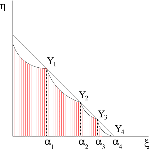
Figure 1: A Young diagram in the $(\xi,\eta)$ plane. Only the points touching the line $\xi+\eta=1$ contribute in the leading order in the large-$n$ limit.

We are interested in calculating the large $n$ behavior of $d_{r}$ and $\frac{{\rm ch}_{r}(\mathbf{2})}{d_{r}}$. This could be done by expressing these quantities in terms of the functions $\varphi(\xi)$ and $\psi(\eta)$, namely by using the logarithmically rescaled variables $\xi$ and $\eta$. However we prefer to calculate separately the contributions of each portion $Y_{t}$ by rescaling the discrete variables $i$ and $j$ with the appropriate power of $n$, thus effectively ”blowing up” each subdiagram $Y_{t}$, which in Fig. 1 is represented by a single point. In this way we are able to calculate $d_{r}$ and $\frac{{\rm ch}_{r}(\mathbf{2})}{d_{r}}$ up to the next to leading order, which differs from the leading one only by a $\log n$ factor and which depends not just from the area $z_{t}$ of $Y_{t}$ but also from its ”shape”. Although not relevant for obtaining the results described in the present paper this next-to-leading order will be important for any further analysis of the model, as discussed in the conclusions. The details of the calculation are given in Appendix A, here we give just the results which are useful for the present discussion.

The large $n$ behavior of $d_{r}$ is given in terms of the areas $z_{t}$ of the subdiagrams $Y_{t}$ by the formula:

$$\log d_{r}=n\log n\left\{1/2z_{1/2}+\sum_{t:\alpha_{t}<1/2}\alpha_{t}z_{t}+\sum_{t:\alpha_{t}>1/2}(1-\alpha_{t})z_{t}\right\}+o(n\log n)$$ (28)

where $z_{1/2}$ is short for $z_{t}$ with $\alpha_{t}=1/2$. As for $\frac{{\rm ch}_{r}(\mathbf{2})}{d_{r}}$ its large $n$ behavior is dominated by the subdiagrams (which we shall denote by $Y_{0}$ and $Y_{1}$) corresponding to a scaling power $\alpha=0$ and $\alpha=1$ respectively. All other contributions, coming from subdiagrams $Y_{t}$ with $\alpha_{t}$ different from $0$ or $1$, are depressed by a factor $n^{-\alpha_{t}}$ if $\alpha_{t}\leq 1/2$ or $n^{\alpha_{t}-1}$ if $\alpha_{t}\geq 1/2$, and can be neglected in the large $n$ limit. $Y_{0}$ (resp. $Y_{1}$) consists of a finite number of columns (resp. rows) of lengths $r_{i}$ (resp. $s_{j}$) proportional to $n$, namely:

$$r_{i}=nf_{i}~{}~{}~{}~{}~{}~{}s_{j}=ng_{j}$$ (29)

where $f_{i}$ and $g_{j}$ are finite in the large $n$ limit. Clearly the areas $z_{0}$ and $z_{1}$ of $Y_{0}$ and $Y_{1}$ are given in terms of $f_{i}$ and $g_{j}$ by:

$$z_{0}=\sum_{i}f_{i},~{}~{}~{}~{}~{}~{}z_{1}=\sum_{j}g_{j}$$ (30)

The large $n$ limit of the leading term of $\frac{{\rm ch}_{r}(\mathbf{2})}{d_{r}}$ can now be easily deduced from (21) and (29) and it is the given by:

$$\frac{{\rm ch}_{r}(\mathbf{2})}{d_{r}}=\sum_{i}f_{i}^{2}-\sum_{j}g_{j}^{2}+o(1)$$ (31)

Notice that $z_{0}$ and $z_{1}$ do not appear at the r.h.s. of (28) because their coefficients vanish. In conclusion, while the leading term of $\frac{{\rm ch}_{r}(\mathbf{2})}{d_{r}}$ depends only on $Y_{0}$ and $Y_{1}$ the leading term of $\log d_{r}$ depends only on the $Y_{t}$’s with $\alpha_{t}$ different from $0$ and $1$.

In order to find the representation $r$ that gives the leading contribution in the large $n$ limit to the partition functions described in the previous section, we can then proceed in the following way: first find separately the extrema of $\frac{{\rm ch}_{r}(\mathbf{2})}{d_{r}}$ and $\log d_{r}$ at fixed $\hat{z}$ defined by

$$\hat{z}\equiv z_{0}+z_{1}$$ (32)

and then find the extremum in $\hat{z}$. The extrema of $|\frac{{\rm ch}_{r}(\mathbf{2})}{d_{r}}|$ and $\log d_{r}$ are a direct consequence of (31) and (28) respectively. For $|\frac{{\rm ch}_{r}(\mathbf{2})}{d_{r}}|$ the extremum corresponds either to $f_{1}=\hat{z}$ or to $g_{1}=\hat{z}$, with all the other coefficients $f_{i}$ and $g_{j}$ equal to zero. In other words either $Y_{0}$ is a diagram consisting of a single column of length $\hat{z}$, or $Y_{1}$ is a diagram with a single row of length $\hat{z}$. In both cases we have

$$|\frac{{\rm ch}_{r}(\mathbf{2})}{d_{r}}|=\hat{z}^{2}$$ (33)

For $\log d_{r}$ it is clear from (28) that the maximum, at fixed $\hat{z}$, occurs when the whole contribution comes from a diagram with $\alpha=1/2$, namely from a Young subdiagram where both rows and columns scale as $n^{1/2}$. The leading term is then:

$$\log d_{r}=\frac{1}{2}n\log n(1-\hat{z})$$ (34)

.

3.2 Phase transitions

Consider first the partition function (13) on a sphere, namely at $G=0$. This can be written as:

$$Z_{n,G=0,p}=\frac{1}{n!^{2}}\sum_{r}e^{2\log d_{r}+p\log\left[\frac{{\rm ch}_{r}(\mathbf{2})}{d_{r}}\right]}$$ (35)

In the large $n$ limit the exponent at the r.h.s. of (35) can be approximated to the leading term by using (33) and (34). Moreover, as the number of representations only grows like the number of partitions of $n$, namely in the large $n$ limit as $e^{\sqrt{n}}$, their entropy is negligible compared to the leading term in (35), and the sum over all representations is given by the contribution of the representation for which the exponent is maximum. As discussed in the previous Section such representation is parametrized by $\tilde{z}$, and we are led to the problem of finding the maximum, with respect to variations of $\tilde{z}$, of

$$n\log n\left[1-\tilde{z}+2A\log\tilde{z}\right]$$ (36)

where, in order to have both terms of the same order in the large $n$ limit, we have set

$$p=An\log n$$ (37)

The maximum of (36) is at $\tilde{z}=2A$. This solution however is valid only for $A<1/2$, as the value of $\tilde{z}$ is limited to the interval $(0,1)$. So the model has two phases: for $A<1/2$ the Young diagram of the leading representation consists of a single row (or column) of length $2An$ and a part of area $(1-2A)n$ whose rows and columns scale like $n^{1/2}$. For $A>1/2$ the sum over the representations is dominated by the representation consisting of a single row (or column) of length $n$.

Let us consider now the more general model whose partition function is given in (16). A difference with respect to the previous case is that $p$ does not need to be even, and the symmetry with respect to the exchange of rows and columns in the representations is broken. So for each value of $\tilde{z}$ there are two representations, whose contribution differ for the sign of ${\rm ch}_{r}(\mathbf{2})$. It easy to check from (16) that the contributions coming from representations with positive sign of ${\rm ch}_{r}(\mathbf{2})$ are always greater in absolute value, and give rise to the leading term in the large $n$ limit. The leading representation is then obtained by finding the value of $\tilde{z}$, constrained by $0\leq\tilde{z}\leq 1$, for which

$$n\log n\left[1-\hat{z}+A\log\left(1-x+x\hat{z}^{2}\right)\right]$$ (38)

is maximum. The phase structure is more complicated than in the previous case, and it is represented in the $(x,A)$ plane in Fig. 2. The phase labeled in the figure with I corresponds to $\hat{z}=0$, namely to a situation where the dominant representation is entirely made of rows and columns that scale as $n^{1/2}$. This phase did not exist in the previous case ($x=1$) except for the trivial point $A=0$.

Figure 2: Phase diagram in the $(x,A)$ plane. The phase transitions between phases I/III and II/III are first order, while the II/III transition is second order.

Phase II and III are the ones already studied at $x=1$ and correspond respectively to $0<\tilde{z}<1$ and $\tilde{z}=1$. The critical line that separates I from III can be easily calculated, and is given by:

$$A_{I,III}=-\frac{1}{\log(1-x)}$$ (39)

while the critical line separating phase II and III is simply:

$$A_{II,III}=\frac{1}{2x}$$ (40)

Finally the line that separates phase I and phase II is given by

$$A_{I,II}=\sqrt{\frac{1-x}{\varphi x}}$$ (41)

where $\varphi$ can be expressed in terms of the coordinate $x_{c}$ of the triple point: $\varphi=4x_{c}(1-x_{c})$. The triple point is at the intersection of (39) and (40)and its coordinate $x_{c}$ is the solution of the transcendental equation $\log(1-x)+2x=0$. Its numerical value is $x_{c}=0.796812..$, from which one also obtains $\varphi=0.647611..$. The critical line (40) is what one expects, according to the results of the $x=1$ model, from an effective number of branch points equal to the number of plaquettes $An\log n$ times the probability $x$ for a plaquette to have a branch point. However the phase diagram discussed above shows that such naive expectation is not fulfilled everywhere. This can be understood by calculating the large $n$ limit of (16) in a slightly different way. We first expand the binomial in (16) and write:

$$Z_{n,G=0,p}(x) = \sum_{r}\sum_{k=0}^{p}\left(\frac{d_{r}}{n!}\right)^{2}\left(\begin{array}[]{c}p\\ k\end{array}\right)(1-x)^{p-k}x^{k}\left(\frac{{\rm ch}_{r}(\mathbf{2})}{d_{r}}\right)^{k}$$ (44)

$$= \sum_{k=0}^{p}\left(\begin{array}[]{c}p\\ k\end{array}\right)(1-x)^{p-k}x^{k}Z_{n,G=0,k}$$ (47)

In the large $n$ limit we parametrize $p$ as in (37), and $k$ as $k=\lambda p$. The sum over $k$ is replaced by an integral over $\lambda$ that can be evaluated using the saddle point method. In doing this the large $n$ solution for $Z_{n,G=0,k}$ must be used, keeping in mind that this consists of two phases, one for $2\lambda A>1$ and one for$2\lambda A<1$. The calculation reproduces the phase diagram of Fig. 2. The saddle point corresponds to $\lambda=0$ in phase I, to $\lambda=x$ in phase III and to $0<\lambda<x$ in phase II. The free energy in the different phases can be obtained from (38) by replacing $\tilde{z}$ with the relevant saddle point solution. So we have:

$$F_{n}(A,x)=n\log n\left[1-z(A,x)+A\log[1-x+xz(A,x)^{2}]\right]$$ (48)

where $z(A,x)=0$ if the point $(A,x)$ is in I, $z(A,x)=1$ if $(A,x)$ is in III, while for $(A,x)$ in II we have

$$z(A,x)=A+\sqrt{A^{2}-\frac{1-x}{x}}$$ (49)

As the free energy is known exactly in the large $n$ limit in any point of the $(A,x)$ plane, the order of the phase transitions can be explicitly calculated. The (I,II) and the (I,III) phase transitions are of first order, while the (II,III) phase transition is a second order phase transition with the second derivative of $F_{n}(A,x)$ with respect to $A$ finite everywhere but with a discontinuity at the critical point $A=1/2x$. The three phases are characterized by different connectivity properties of the world sheet. We have not been able to investigate these properties within the variational approach, so we have to rely on the equivalence between gauge theories of $S_{n}$ and random walks on one hand, and between random walks and random graphs on the other. These will be discussed in the following sections; in particular the connectivity of the world sheet in the different phases is discussed in Section 4.3, as a corollary of well known results in the theory of random graphs.

Finally let us consider the model given by the partition function (11). As already pointed out, this coincides with the small $x$ limit of (16) provided we put ${\cal A}=xp=xAn\log n$. For small $x$ the first order phase transition occurs at $A=-\frac{1}{\log(1-x)}$, hence for (11) at ${\cal A}=n\log n$.

4 Gauge theories on a disk as random walks on the group manifold

A two-dimensional gauge theory on a disk is equivalent to a random walk on the gauge group manifold, the area of the disk being identified with the number of steps and the gauge theory action with the transition probability at each step.

This result is completely general with respect to the choice of the gauge group and of the action, as we will prove below. However it might be useful to show first how this result emerges in the $S_{n}$ gauge theory defined by Eq.(13), that is in a theory where all plaquettes variables are forced to be equal to transpositions.

Suppose we want to compute such partition function on a disk with a fixed holonomy $Q\in S_{n}$, Eq. (18). The latter shows that the partition function depends only on the holonomy $Q$ and the area of the disk (that is the theory is invariant for area-preserving diffeomorphism). It follows that we can freely choose any cell decomposition of the disk made of $p$ plaquettes, e.g. the one shown in Fig. 3.

Figure 3: A cell decomposition of the disk. The permutations on the dashed links have been gauge-fixed to the identity, so that the ones on the boundary are forced to be transpositions. The ordered product of the $p$ transpositions gives the holonomy.

To compute the partition function means to count the ways in which we can place permutations $P$ on all the links in such a way that

• the ordered product of the links around each plaquette is a transposition

• the ordered product of the links around the boundary of the disk is a permutation in the same conjugacy class as $Q$

Now we can use the gauge invariance of the theory to fix all the radial links to contain the identical permutation. At this point the links on the boundary are forced to contain transpositions: therefore the partition function with holonomy $Q$ is the number of ways in which one can write the permutation $Q$ as an ordered product of $p$ transpositions. This in turn can be seen as a random walk on $S_{n}$, in which, at each step, the permutation is multiplied by a transposition chosen at random: the gauge theory partition function for area $p$ and holonomy $Q$ is the probability that after $p$ steps the walker is in $Q$.

4.1 The correspondence for a general gauge theory

To show that this result actually holds for all gauge groups and choice of the action, consider now a gauge theory on a disk of area $p$ with gauge group $G$ and holonomy $g\in G$ on the disk boundary. To fix the notations, we will consider a finite group $G$, but the argument can be extended to Lie groups. The theory is defined by a function $w(g)$ such that the Boltzmann weight of a configuration is given by the product of $w(g_{pl})$ over all plaquettes of the lattice, with $g_{pl}$ the ordered product of the links around the plaquette. For the theory to be gauge invariant, $w$ has to be a class function; moreover we will require $w(g)\geq 0$ for all $g$ and normalize $w$ so that $\sum_{g}w(g)=1$.

The partition function is [14, 15]

$$Z_{p}(g)=\frac{1}{|G|}\sum_{r}d_{r}\tilde{w}_{r}^{p}\chi_{r}(g)$$ (50)

where the sum is over all irreducible representations of $G$, $\chi_{r}(g)$ is the character of $g$ in the representation $r$, and the $\tilde{w}_{r}$’s are the coefficients of the character expansion of the Boltzmann weight:

$$w(g)=\frac{1}{|G|}\sum_{r}d_{r}\tilde{w}_{r}\chi_{r}(g)$$ (51)

Now consider a random walk on $G$ with transition probability defined as follows: if the walker is in $g_{p}\in G$ at step $p$, then its position at step $p+1$ is obtained by left multiplying $g_{p}$ by an element $g$ chosen in $G$ with a probability $t(g)$ which is a class function, i.e. depends on the conjugacy class of $g$ only.

Suppose the random walks starts in the identity of $G$, and call $K_{p}(g)$ the probability that the walker is in $g$ after the $p$-th step. Then

$$K_{p+1}(g)=\sum_{g^{\prime}}t(g^{\prime}g^{-1})K_{p}(g^{\prime})$$ (52)

Now assume $K_{p}(g)$ is a class function, with character expansion

$$K_{p}(g)=\frac{1}{|G|}\sum_{r}d_{r}k^{(p)}_{r}\chi_{r}(g)$$ (53)

then it follows form Eq. (52) that also $K_{p+1}$ is a class function, and the coefficients of its character expansion are

$$k^{(p+1)}_{r}=\tilde{t}_{r}k^{(p)}_{r}$$ (54)

where the $\tilde{t}_{r}$’s are the coefficients of the character expansion of the class function $t$:

$$t(g)=\frac{1}{|G|}\sum_{r}d_{r}\tilde{t}_{r}\chi_{r}(g)$$ (55)

Now, since $K_{1}(g)=t(g)$, it follows by induction that $K_{p}$ is indeed a class function, and

$$k^{(p)}_{r}=\tilde{t}_{r}^{p}$$ (56)

so that the probability distribution after $p$ steps of the random walk equals the gauge theory partition function $Z_{p}(g)$ provided the Boltzmann weight of the plaquette in the latter is identified with the transition function of the former:

$$w(g)=t(g)$$ (57)

In conclusion, the partition function of a gauge theory on a disk, of area $p$ with a certain holonomy $g$ on the disk boundary, equals the probability that a random walk that starts in the identity of the group will reach the element $g$ in $p$ steps, each step consisting of left multiplication by an element chosen with a probability distribution coinciding with the plaquette Boltzmann weight of the gauge theory.

4.2 Cutoff phenomenon in random walks on $S_{n}$

The cutoff phenomenon in random walks was discovered in Ref.[13], where a random walk on $S_{n}$ was studied in which at each step the permutation is multiplied by the identical permutation with probability $1/n$ and by a randomly chosen transposition otherwise. According to the argument of the previous section, this corresponds to our model Eq.(16) with $x=1-1/n$. The holonomy of the gauge theory translates into constraints on the element of $S_{n}$ where the random walk ends: for example the partition function on the sphere will count the walks that return to the identical permutation in $p$ steps.

The main result of Ref.[13] is that if the number of steps scales as $An\log n$, then in the large-$n$ limit for $A>1/2$ the probability of finding the walker in any given element $Q\in S_{n}$ is just $1/n!$ for all $Q$: complete randomization has been achieved and all memory of the initial position of the walker has been erased.

In terms of the corresponding gauge theory, this can be translated into a statement about the partition function on a disk: for $A>1/2$, the partition function with any given holonomy $Q$ stops depending on $A$ and is simply proportional to the number of permutations in the conjugacy class of $Q$. This is true in particular for $Q=1$, corresponding to the partition function on the sphere. Therefore the phase transition found in Sec. 3 has a natural interpretation as a cutoff phenomenon in the corresponding random walk.

Strictly speaking, this applies only to the specific model $x=1-1/n$ studied in Ref.[13]. However we want to argue that this is the correct interpretation of the whole line of phase transitions at $A=\frac{1}{2x}$ found in Sec. 3. Consider first the model with $x=1$, where at each step the permutation is multiplied by a random transposition. The probability distribution does not have a limit as the number of steps goes to infinity, since for even number of steps one can only obtain an even permutation and vice versa. Therefore the probability distribution in $S_{n}$ can never become uniform. However it is natural to expect that a sort of cutoff phenomenon occurs all the same at number of steps $p=1/2\ n\log n$, and precisely that for even $p$ the probability distribution becomes uniform in the alternating group and for odd $p$ in its complement.

To support this conjecture, let us compute e.g. the expected number of cycles of length 1 in the permutation obtained after $p$ steps. The calculation is described in Appendix B, and the result is

$$N_{1}(x=1,p)=1+(n-1)\left(\frac{n-3}{n-1}\right)^{p}$$ (58)

so that for $p=An\log n$ we have

$$N_{1}(x=1)\sim\left\{\begin{array}[]{cc}n^{1-2A}&{\rm for}\ A\leq 1/2\\ 1&{\rm for}\ A>1/2\end{array}\right.$$ (59)

The result for $A>1/2$ is the one expected for a uniform probability distribution in the alternating group or its complement.

Repeating the calculation for arbitrary $x$ one finds

$$N_{1}(x)\sim\left\{\begin{array}[]{cc}n^{1-2xA}&{\rm for}\ A\leq 1/(2x)\\ 1&{\rm for}\ A>1/(2x)\end{array}\right.$$ (60)

so that the cutoff phenomenon occurs at $A=1/(2x)$, the result one intuitively expects from the fact that a fraction $x$ of the random walk steps are “wasted” in doing nothing and do not contribute to the randomization process.

4.3 Results from random graphs theory

In the previous sections we have mainly considered the theory defined on a sphere: we have found a complex phase structure with first and second-order phase transitions. One of the transition lines can be interpreted as a cutoff phenomenon in the corresponding random walk.

In this section we consider the theory with free boundary conditions: the permutations on the boundary of the disk are summed over like the internal ones. From the point of view of the random walk, this implies considering all the possible paths irrespective of the permutation they end in after $p$ steps. We will exploit a correspondence between cutoff phenomena in random walks and phase transitions in random graphs first noted in Ref. [16]. Consider the random walk in $S_{n}$ defined by $x=1$, i.e. at each step the permutation is multiplied by a random transposition (but all the arguments we will give translate trivially to the case $x<1$). From the point of view of coverings, a step in which the transposition $(ij)$ is used corresponds to adding a simple branch point that connects the two sheets $i$ and $j$ of the covering surface. One can think of the process as the construction of a random graph on $n$ sites where at each step a link between two sites is added at random. After $p=An\log n$ steps the expected number of links is equal to the number of steps (since the number of available links is $O(n^{2})$ the fact that the same link can be added more than once can be neglected in the large $n$ limit; see Ref. [16]).

It is a classic result in the theory of random graphs [18, 19] that if the number of links $p$ is smaller than $1/2\ n\log n$ then the graph is almost certainly disconnected while for $p>1/2\ n\log n$ the graph is almost certainly connected, where “almost certainly” means that the probability is one in the limit $n\to\infty$. Therefore we conclude that the model with free boundary conditions undergoes a phase transition at $A=1/2$ where the covering surface goes from disconnected to connected. For $x<1$, the same transition occurs at $A=1/(2x)$.

Notice that the free boundary conditions are crucial for this argument to work: in the case, say, of the sphere, the corresponding random walk is forced to go back to the initial position in $p$ steps, so that links in the graph are not added independently and the result of Ref.[18, 19] do not apply. However some consequences can be drawn from these results also for the case of the sphere. Consider first the model with $x=1$ and a sphere of area $A>1$. The latter can be thought of as two disks, both with area $A>1/2$, joined together. The partition function of the sphere is then obtained by multiplying together the partition functions of the two disks and by summing over the common holonomy $P$ on the border. If the world sheets of the two disks are almost certainly connected, the same applies to the world sheet of the resulting sphere. Strictly speaking this proof holds only for $A>1$, however we have shown that the leading term of order $n\log n$ of the free energy is independent of $A$ for $A>1/2$. So unless a phase transition occurs due to the next leading term of order $n$ (which cannot be ruled out a priori) the whole phase with $A>1/2$ at $x=1$ (and extending the argument to $x<1$ the whole phase III) will be characterized by a connected world sheet. What can be said about phase II and I? We mentioned already the result in the theory of random graphs that for a number of links $p$ smaller than $1/2n\log n$ the graph is almost certainly disconnected. Although this result applies to the case of free boundary conditions, it should a fortiori be true also for the sphere. In fact the sphere corresponds to a random walk which is forced to end in the identical permutation, thus favoring graphs in which less links are turned on. So for $A<1/2$ at $x=1$, namely in phase II, and a fortiori in phase I we expect the world sheet to be disconnected. Another result in random graphs [18, 19] states that if the number of links $p$ grows like $\epsilon n\log n$ with $\epsilon>0$, the size $n_{c}$ of the largest connected graph is $n$ in the large $n$ limit, namely $\lim_{n\rightarrow\infty}n_{c}/n=1$. Again, although the result is proved for graphs corresponding to random walks with free boundary conditions, it can be extended, at $x=1$, to a sphere of area $\epsilon n\log n$ which can be thought of as obtained by sewing two disks of area $\epsilon/2n\log n$. Both phase III and phase II are then characterized by the presence of a connected world sheet of size $n_{c}\sim n$ in the large $n$ limit, but phase III has completely connected world sheets while phase II has not. In phase I the number of effective branch points grows slower than any $\epsilon n\log n$, possibly like $\alpha n$. If that is the case (a detailed analysis of next to leading terms would be required to check this point) then another result [18, 19] of random graphs could be applied. This states that if the number of links is $\alpha n$ in the large $n$ limit, then for $\alpha>1/2$ the largest connected part has size $\psi(\alpha)n$ with $\psi(1/2)=0$ and $\psi(\infty)=1$. The function $\psi(\alpha)$ is known and can be written as an infinite series. The point $\alpha=1/2$ is the percolation threshold, its existence may be an indication of further phase structure within phase I.

5 Relation with two dimensional Yang-Mills theories

Besides being linked to the theory of random walks and random graphs, $S_{n}$ gauge theory is also closely related to lattice $U(N)$ gauge theories on a Riemann surface. This was first discovered by Gross and Taylor  [4, 5] , who found that the coefficients of the large $N$ expansion of the $U(N)$ partition function could be interpreted in terms of string configurations, namely of coverings of the Riemann surface. In the case of $U(N)$ Yang-Mills theory the maps from the string world sheet to the target space have two possible orientations and world sheets of opposite orientations can interact only through point-like singularities. As a result the theory almost exactly factorizes into two copies of a simpler, orientation preserving chiral theory. This chiral Yang-Mills theory is obtained as a truncation of the whole theory by restricting the sum over the irreducible representations of $U(N)$ to the representations whose Young diagram contains a finite number of boxes in the large $N$ limit. The number $n$ of boxes in a representation coincides with the number of times the world sheet of the corresponding string configuration covers the target space. While in the gauge theory of $S_{n}$ the irreducible representations are labeled by Young diagrams that contain exactly $n$ boxes, in chiral $U(N)$ gauge theory the irreducible representations are labeled by Young diagrams which contain an arbitrary number of boxes and are only restricted by the condition that the number of rows do not exceed $N-1$.

The partition function of chiral Yang-Mills theory can then be written as a sum over $n$, and we expect each term in the sum, being the number of $n$-coverings, to be related to an $S_{n}$ gauge theory. For chiral Yang-Mills this is true only on a torus, namely if the genus of the target space is zero. It is well known in fact that for different genuses the coefficients of the $1/N$ expansion of the $U(N)$ partition function are not directly related to the number of coverings, due to presence of the so called $\Omega^{-1}$ points.

A matrix model that gives, to all orders in the $1/N$ expansion, the exact statistic of branched coverings on a Riemann surface and whose restriction to a fixed value of $n$ coincides with a $S_{n}$ gauge theory was introduced by Kostov, Staudacher and Wynter (KSW in short) in [1, 2]. This model has still a $U(N)$ gauge invariance but realized in terms of complex rather than unitary $N\times N$ matrices. The partition function of the KSW model on a Riemann surface of genus $G$ is [1, 2]:

$$Z_{N,G}^{(KSW)}(\tau,\mu)=\sum_{n}\sum_{r\in U(N),|r|=n}\left(N^{n}\frac{d_{r}}{n!}\right)^{2-2G}\exp\left[\frac{\tau n(n-1)}{2N}\frac{{\rm ch}_{r}(\mathbf{2})}{d_{r}}-n\mu\right]$$ (61)

where we denote by $r$ both the Young diagrams and the corresponding representations of either $U(N)$ of $S_{|r|}$, with $|r|$ the number of boxes in $r$. The sum is over all Young diagrams corresponding to representations of $U(N)$, $d_{r}$ and ${\rm ch}_{r}(\mathbf{2})$ are the same as in the previous sections. By comparing (61) with (11) we can write:

$$Z_{N,G}^{(KSW)}(\tau,\mu) = Z_{1,G}({\cal A})N^{2-2G}e^{-\mu}+Z_{1,G}({\cal A})N^{2(2-2G)}e^{-2\mu}+\ldots$$ (62)

$$+ Z_{N,G}({\cal A})N^{N(2-2G)}e^{-N\mu}+\tilde{Z}_{N+1,G}({\cal A})N^{(N+1)(2-2G)}e^{-(N+1)\mu}+\ldots$$

The partition functions at the r.h.s. of (62), for $n\leq N$, are the partition functions of the $S_{n}$ gauge theory given in (11) with ${\cal A}=\frac{\tau n(n-1)}{2N}$. For $n>N$ the partition functions, denoted by $\tilde{Z}$, are incomplete $S_{n}$ partition functions, because in that case some irreducible representations of $S_{n}$, whose Young diagram has more than $N$ rows, do not correspond to any representation of $U(N)$.

The partition function of chiral Yang-Mills theory is similar to (61), but with the dimension $\Delta_{r}$ of the $U(N)$ representation replacing the factor $N^{n}\frac{d_{r}}{n!}$ at the r.h.s.. The ratio between these two factors is the so called $\Omega_{r}$ term, whose presence prevents chiral Yang-Mills theory from having a simple interpretation in terms of coverings for $G\neq 1$.

In spite of these differences two dimensional Yang-Mills theory, chiral Yang-Mills theory and the KSW model all share some common features in the large $N$ limit. If the target space has the topology of a sphere ($G=0$) all these theories exhibit a non trivial phase structure in the large $N$ limit. In the case of two dimensional Yang-Mills theory there is a third order phase transition, the Douglas-Kazakov phase transition  [8]. This occurs at a critical value ${\cal{A}}=\pi^{2}$ of the area of the sphere, measured in units of the coupling constant. This phase transition is well understood in terms topologically non trivial configurations  [9, 10]. The phase structure of chiral Yang-Mills theory and of the KSW model has been studied in  [2] and in  [12] and it turns out to be richer than pure Yang-Mills. In the KSW model four distinct phases are present in the $(\tau,\mu)$ plane. In all these cases the saddle point in the large $N$ limit corresponds to a representation of $U(N)$ where both row and columns of the associated Young diagram scale as $N$, hence the total number of boxes is of order $N^{2}$:

$$n\propto N^{2}$$ (63)

This means that the saddle point at large $N$ corresponds to a string configuration that covers the target space a number of times $n$ proportional to $N^{2}$, and that the associated Young diagram has rows and columns of order $\sqrt{n}$. Besides the free energy is of order $N^{2}$, namely of order $n$. This also means that the number of branch points $p$ if of order $n$. In fact the free energy is the exponent at the r.h.s. of (61) calculated at the saddle point plus a term, that does not depend from the number of branch points, coming from the dimension of the representation. Let us expand the exponential in (61) in power series:

$$\exp\left[\frac{\tau n(n-1)}{2N}\frac{{\rm ch}_{r}(\mathbf{2})}{d_{r}}-n\mu\right]=\sum_{p}\frac{1}{p!}\left[\frac{\tau n(n-1)}{2N}\frac{{\rm ch}_{r}(\mathbf{2})}{d_{r}}-n\mu\right]^{p}$$ (64)

Each term in the sum at the r.h.s. corresponds to a configuration with $p$ plaquettes, each plaquette with either a single quadratic branch point or no branch point at all with probabilities respectively proportional to $\frac{\tau n(n-1)}{2N}$ and $n\mu$. The former grows faster with $n$ than the latter, so in the large $n$ limit the probability $x$ of having a branch point in each plaquette tends to 1.

Finally we remark that the sum over $p$ in (64) is dominated at large $n$ by by a single value of $p$ , namely $p=\left[\frac{\tau n(n-1)}{2N}\frac{{\rm ch}_{r}(\mathbf{2})}{d_{r}}-n\mu\right]$. This implies that $p$ is also of order $n$. To summarize: the standard large $N$ limit of $U(N)$ gauge theories is described in terms of string configurations (coverings), which are also configurations of an $S_{n}$ gauge theory, with $n$ given by (63), rows and columns scaling like $\sqrt{n}$ and

$$p\propto n,~{}~{}~{}~{}~{}~{}~{}~{}~{}x=1$$ (65)

That means the large $N$ limit of $U(N)$ gauge theories corresponds to the point at the right corner of region I in Fig. 2, where the coefficient of $n\log n$ in $p$ is strictly zero. In order to ”blow up” that point and determine weather a further phase structure is present there one would need to evaluate the terms of order $n$ in the free energy. This will be the task of a future work. We just remark here that the presence of a non trivial phase structure in that region is likely for at least two reasons: because that region is the section with a constant $n$ plane of the large $N$ limit of the KSW model, which has a non trivial phase structure, and because we know from the random graphs theory that for $p\propto n$ there is at least one transition, the percolation transition.

It appears from the previous discussion that the phase transition that we found in the $S_{n}$ theory, and that corresponds to the well known cutoff phenomenon in random walk, does not have a counterpart among the known phase transitions in two dimensional Yang-Mills theory. It is quite natural to ask weather a transition of this kind exists also for two dimensional Yang-Mills and other $U(N)$ gauge theory on a sphere. We found the answer to be affirmative. This new type of phase transition, the cutoff phenomenon, can be observed provided the coupling constant is rescaled with $N$ with an extra $\log N$ with respect to the usual ’t Hooft prescription. We give here a simple, although rigorous, argument, leaving a detailed analysis of the transition to a future work. Consider the partition function of YM2 on a sphere (see for instance  [10]) with gauge group $U(N)$:

$$Z_{0}(A,N)=e^{-\frac{A}{24}(N^{2}-1)}\sum_{n_{1}>n_{2}>...>n_{N}}\Delta^{2}(n_{1},...,n_{N})e^{-\frac{A}{2N}\sum_{i=1}^{N}n_{i}^{2}}$$ (66)

where the $n_{i}$’s are integers, $\Delta(n_{1},...,n_{N})$ is the Vandermonde determinant and $A$ the area of the sphere. In the large $N$ limit a la ’t Hooft $A$ is kept fixed. We are going to allow $A$ to rescale with $N$: $A\rightarrow A(N)$. For $A(N)$ sufficiently large we expect the sum to be dominated in the large $N$ limit by the configuration for which the exponential is maximum, namely $\{n_{1},n_{2},.....n_{N}\}=\{\frac{N-1}{2},\frac{N-1}{2}-1,....-\frac{N-1}{2}\}$. This configuration corresponds to the trivial representation of $U(N)$, and it is the exact analogue of the representation of $S_{n}$ consisting of a single row. Let us determine now the value of $A(N)$ for which this configuration ceases to be a maximum by comparing its contribution to the sum in (66) with the contribution of a configuration where $n_{1}$ is increased of one unit. We find:

$$\frac{\Delta^{2}(n_{1},...,n_{N})e^{-\frac{A}{2N}\sum_{i=1}^{N}n_{i}^{2}}|_{\{n_{1},n_{2},.....n_{N}\}=\{\frac{N-1}{2},\frac{N-1}{2}-1,....-\frac{N-1}{2}\}}}{\Delta^{2}(n_{1},...,n_{N})e^{-\frac{A}{2N}\sum_{i=1}^{N}n_{i}^{2}}|_{\{n_{1},n_{2},.....n_{N}\}=\{\frac{N-1}{2}+1,\frac{N-1}{2}-1,....-\frac{N-1}{2}\}}}=\frac{e^{\frac{A(N)}{2}}}{N^{2}}$$ (67)

The cutoff phenomenon occurs when the r.h.s. of (67) is greater than $1$, namely for $A(N)>4\log N$, while for $A(N)<4\log N$ we are in presence of a new phase whose characteristics are still to be determined.

6 Conclusions

Let us summarize the results obtained in the paper. We have studied a two-dimensional gauge theory of the symmetric group $S_{n}$ that describes the statistics of branched coverings on a Riemann surface, in the large-n limit.

• The theory on the sphere shows an interesting phase diagram when the number of branch points scales as $n\log n$, with lines of first and second-order phase transitions.

• All two-dimensional gauge theories on a genus-0 surface can be mapped into random walks in the corresponding group manifold. In our case, this allows us to interpret one of the transition lines as a cutoff phenomenon in the corresponding random walk.

• The theory on a disk, with free boundary conditions, can be studied with methods of the theory of random graphs: this allows one to show that there is a phase transition on a disk from a disconnected to a connected covering surface. From this one can argue, and with some limitations prove, that the connectedness of the covering is what characterizes the different phases also on the sphere.

• A cutoff phenomenon is found also in 2D Yang-Mills on a sphere, if the area of the sphere scales with $N$ like $N\log N$

The present paper can be extended in two distinct directions. On one hand it would be desirable to understand better region I of the phase diagram of Fig. 2, and in particular its right corner which corresponds to the large $N$ limit of $U(N)$ gauge theories. For this purpose the variational approach should be implemented to include the contributions of the next-to-leading order in $n$, which is of order $n$ instead of $n\log n$. This might reveal further phase structure, like for instance a percolation phase transition. Also, phase transitions in region I should be the analogue in $S_{n}$ gauge theory of the Douglas-Kazakov phase transition in 2D Yang-Mills, and of the phase transitions studied in [12] and [2] for chiral Yang-Mills and KSW model respectively. It can be shown that the calculation of the correlators, which are relevant in order to determine the order parameters of the various phase transitions, also requires to know the free energy beyond the leading order.

The existence of a cutoff phenomenon in two dimensional Yang-Mills, although within the framework of a non conventional scaling with $N$ of the coupling constant, is also a fact whose meaning and physical implications, if any, should be further investigated. In particular a full description of the phase preceding the cutoff is still lacking.

Acknowledgments

We are grateful to M. Billó and M. Caselle for many enlightening conversations.

Appendix A

In this appendix we calculate in the large $n$ limit some relevant quantities, such as $\log d_{r}$ and $\frac{{\rm ch}_{r}(\mathbf{2})}{d_{r}}$, in a representation $r$ associated to a Young diagram whose rows and columns scale respectively as $n^{\alpha}$ and $n^{1-\alpha}$. This is not the most general case. However we have already shown in Section 3 that in the large $n$ limit the most general Young diagram can be decomposed into a discrete set of subdiagrams $Y_{t}$ (see Fig. 1 and related discussion), each scaling as above with a different power $\alpha_{t}$. The calculation that we are going to present below will also apply to each $Y_{t}$, and the result for the whole Young diagram is obtained by summing the contributions of the different $Y_{t}$’s. The shaded area of the Young diagram in 1 gives contributions which are subleading in the large $n$ and can be neglected. Let us consider first a Young diagram where rows and columns scale respectively as $n^{\alpha}$ and $n^{1-\alpha}$. It is convenient then to introduce the following continuous variables:

$$x=\frac{i}{n^{\alpha}},~{}~{}~{}~{}~{}~{}y=\frac{j}{n^{1-\alpha}}$$ (68)

and correspondingly

$$f(x)=\frac{r_{i}}{n^{1-\alpha}},~{}~{}~{}~{}~{}~{}g(y)\equiv f^{-1}(y)=\frac{s_{j}}{n^{\alpha}}$$ (69)

where the derivatives $f^{\prime}(x)$ and $g^{\prime}(y)$ are everywhere negative or null. The variable $x$ ranges from $0$ to a maximum value $x_{\rm max}=f^{-1}(0)$ and similarly $y$ ranges from $0$ to $y_{\rm max}=f(0)$. Then it is easy to replace the discrete variables with the continuous ones in the expression of $d_{r}$ and $\frac{{\rm ch}_{r}(\mathbf{2})}{d_{r}}$ and obtain:

$$\log d_{r}=\log n!-n\int_{0}^{f^{-1}(0)}dx\int_{0}^{f(x)}dy\log\left\{n^{\alpha}\left(f^{-1}(y)-x\right)+n^{1-\alpha}\left(f(x)-y\right)\right\}$$ (70)

and

$$\frac{{\rm ch}_{r}(\mathbf{2})}{d_{r}}=\frac{1}{1-1/n}\left[n^{-\alpha}\int_{0}^{f^{-1}(0)}dxf(x)^{2}-2n^{\alpha-1}\int_{0}^{f^{-1}(0)}dxxf(x)\right]$$ (71)

while the constraint (19) in the large $n$ limit becomes:

$$\int_{0}^{f^{-1}(0)}dxf(x)=\int_{0}^{f(0)}dyf^{-1}(y)=1$$ (72)

Keeping only the terms of order $n\log n$ and $n$ in eq.s (70) we have for $\log d_{r}$, in the large $n$ limit:

$$\log d_{r} = \alpha n\log n-n\left[1+\int_{0}^{f^{-1}(0)}dxf(x)\left(\log f(x)-1\right)\right]~{}~{}~{}~{}~{}~{}~{}\alpha<1/2$$

$$\log d_{r} = (1-\alpha)n\log n-n\left[1+\int_{0}^{f(0)}dyf^{-1}(y)\left(\log f^{-1}(y)-1\right)\right]~{}~{}~{}~{}~{}~{}~{}\alpha>1/2$$ (73)

Similarly we obtain for $\frac{{\rm ch}_{r}(\mathbf{2})}{d_{r}}$, keeping terms up to order $1$:

$$\log\left[\frac{{\rm ch}_{r}(\mathbf{2})}{d_{r}}\right] = -\alpha\log n+\log\left[\int_{0}^{f^{-1}(0)}dxf(x)^{2}\right]~{}~{}~{}~{}~{}~{}~{}\alpha<1/2$$

$$\log\left[\frac{{\rm ch}_{r}(\mathbf{2})}{d_{r}}\right] = (1-\alpha)\log n+\log\left[\int_{0}^{f(0)}dyf^{-1}(y)^{2}\right]~{}~{}~{}~{}~{}~{}~{}\alpha>1/2$$ (74)

Consider now the most general case, where the Young diagram consists, in the large $n$ limit, of a discrete set of subdiagrams $Y_{t}$, each scaling with a different power $\alpha_{t}$. Each $Y_{t}$ contributes to $\log d_{r}$ with a term of the form (73), with the appropriate $\alpha_{t}$ in place of $\alpha$ and weighted with its area $z_{t}$. The sum over $t$ reproduces, for the leading $n\log n$ term, eq.(28). Consider now $\frac{{\rm ch}_{r}(\mathbf{2})}{d_{r}}$. It is clear from (71) that the asymptotic behavior of the contribution coming from $Y_{t}$ is $n^{-\alpha_{t}}$ (resp. $n^{1-\alpha_{t}}$) for $\alpha_{t}<1/2$ (resp. $\alpha_{t}>1/2$). The sum over $t$ is then dominated by subdiagrams with scaling powers $\alpha=0$ and $\alpha=1$ which are discussed in detail in Section 3.

Appendix B

In this Appendix we derive Eqs. (59) and (60), in two different ways: first by direct combinatorial methods, then using the character expansion of the probability distribution discussed in Subsec 4.1.

Consider a random walk in $S_{n}$ in which, at each step, the permutation is multiplied by a randomly chosen transposition with probability $x$, or by the identity with probability $1-x$. It is convenient to think of $n$ objects and $n$ boxes: initially the object $i$ is in the box $i$. Then we start moving them around with the following rule: At each step, we exchange two randomly chosen objects with probability $x$, or we do nothing with probability $1-x$.

Choose now one of the $n$ objects, say number 1, and compute the probability $P_{1}(x,p)$ that, after $p$ steps, it is in box number 1 (either because it never left it, or because it went back to it). The expected number of cycles of length 1 in the final permutation is then just

$$N_{1}(x,p)=nP_{1}(x,p)$$ (75)

To compute $P_{1}(x,p)$, write it as

$$P_{1}(x,p)=\sum_{k=0}^{p}q(k)s(k)$$ (76)

where $q(k)$ is the probability that object 1 changes box exactly $k$ times during the walk, and $s(k)$ is the probability that it will be back in its original box after changing box $k$ times. We have easily

$$q(k)=\left(p\atop k\right)\left(\frac{2x}{n}\right)^{k}\left(1-\frac{2x}{n}\right)^{p-k}$$ (77)

For $s(k)$ we can write a recursion relation: suppose element 1 is in box 1 after being moved $k$ times: Then it will certainly not be in box 1 after being moved $k+1$ times. If it is not in box $1$ after being moved $k$, times, it will be after being moved $k+1$ times with probability $1/(n-1)$. Hence

$$s(k+1)=\frac{1}{n-1}\left[1-s(k)\right]$$ (78)

that together with the initial condition $s(0)=1$ gives

$$s(k)=\frac{1}{n}\left[1-\frac{1}{(1-n)^{k-1}}\right]$$ (79)

Substituting in Eq. (76) we obtain

$$P_{1}(x,p)=\frac{1}{n}\left[1+(n-1)\left(\frac{n-2x-1}{n-1}\right)^{p}\right]$$ (80)

(this result for $x=1-1/n$ was already quoted in Ref. [13]), and

$$N_{1}(x,p)=1+(n-1)\left(\frac{n-2x-1}{n-1}\right)^{p}$$ (81)

which includes in particular Eq. (59), so that taking the limit $n\to\infty$ with $p=An\log n$ one obtains Eq. (60).

The same result can be obtained with character expansion methods by noticing that $N_{1}(x,p)$ is simply the expectation value $<Tr\ Q>$ of the trace of the permutation obtained after $p$ steps, where the trace is taken in the “fundamental” $n$-dimensional representation: Such representation is reducible to a direct sum of the trivial representation (Young diagram made of one line of $n$ boxes) and the $n-1$ dimensional representation described by a diagram with two rows of length $n-1$ and $1$. Therefore

$$Tr\ Q={\rm ch}_{1}(Q)+{\rm ch}_{n-1}(Q)$$ (82)

Using the character expansion of the probability distribution as in subsec. 4.1 we obtain

$$N_{1}(x,p) = \langle Tr\,Q\rangle$$

$$= \frac{1}{n!}\sum_{Q\in S_{n}}\left[{\rm ch}_{1}(Q)+{\rm ch}_{n-1}(Q)\right]\sum_{r}d_{r}\left[(1-x)+x\frac{{\rm ch}_{r}(\mathbf{2})}{d_{r}}\right]^{p}{\rm ch}_{r}(Q)$$

Using the orthogonality of characters and

$$\frac{{\rm ch}_{n-1}(\mathbf{2})}{d_{n-1}}=\frac{n-3}{n-1}$$ (84)

we find again Eq. (81).

References

- [1] I. K. Kostov and M. Staudacher, Phys. Lett. B394 (1997) 75 [hep-th/9611011].
- [2] I. K. Kostov, M. Staudacher and T. Wynter, Commun. Math. Phys. 191, 283 (1998) [hep-th/9703189].
- [3] M. Billo, A. D’Adda and P. Provero, hep-th/0103242.
- [4] D. J. Gross and W. I. Taylor, Nucl. Phys. B400 (1993) 181 [hep-th/9301068].
- [5] D. J. Gross and W. I. Taylor, Nucl. Phys. B403 (1993) 395 [hep-th/9303046].
- [6] J. Baez and W. Taylor, Nucl. Phys. B 426 (1994) 53 [arXiv:hep-th/9401041].
- [7] M. Billo, A. D’Adda and P. Provero, Unpublished.
- [8] M. R. Douglas and V. A. Kazakov, Phys. Lett. B 319, 219 (1993) [hep-th/9305047].
- [9] M. Caselle, A. D’Adda, L. Magnea and S. Panzeri, arXiv:hep-th/9309107.
- [10] D. J. Gross and A. Matytsin, Nucl. Phys. B 429 (1994) 50 [arXiv:hep-th/9404004].
- [11] D. J. Gross and A. Matytsin, Nucl. Phys. B 437 (1995) 541 [arXiv:hep-th/9410054].
- [12] M. J. Crescimanno and W. Taylor, Nucl. Phys. B 437 (1995) 3 [arXiv:hep-th/9408115].
- [13] P. Diaconis and M. Shahshahani, Z. Wahrsch. Verw. Gebiete 57 (1981) 159.
- [14] A. A. Migdal, Sov. Phys. JETP 42 (1975) 413.
- [15] B. E. Rusakov, Mod. Phys. Lett. A5 (1990) 693.
- [16] I. Pak and V. H. Vu, Discrete Applied Math., 110 (2001) 251.
- [17] D. J. Gross and E. Witten, Phys. Rev. D 21 (1980) 446.
- [18] P. Erdös and A. Rényi, Publ. Math. Debrecen 6 (1959) 290.
- [19] P. Erdös and A. Rényi,“The Art of Counting” (Cambridge:MIT 1973).