HEPHY-PUB 740/01 UWThPh-2001-27 CUQM-86 hep-th/0110220 July 2001

DISCRETE SPECTRA OF SEMIRELATIVISTIC HAMILTONIANS FROM ENVELOPE THEORY
Richard L. HALL
Department of Mathematics and Statistics, Concordia University,
1455 de Maisonneuve Boulevard West, Montréal, Québec, Canada H3G 1M8
Wolfgang LUCHA
Institut für Hochenergiephysik, Österreichische Akademie der Wissenschaften,
Nikolsdorfergasse 18, A-1050 Wien, Austria
Franz F. SCHÖBERL
Institut für Theoretische Physik, Universität Wien,
Boltzmanngasse 5, A-1090 Wien, AustriaAbstract

We analyze the (discrete) spectrum of the semirelativistic “spinless-Salpeter” Hamiltonian

$$H=\beta\sqrt{m^{2}+{\bf p}^{2}}+V(r)\ ,\quad\beta>0\ ,$$

where $V(r)$ is an attractive, spherically symmetric potential in three dimensions. In order to locate the eigenvalues of $H,$ we extend the “envelope theory,” originally formulated only for nonrelativistic Schrödinger operators, to the case of Hamiltonians involving the relativistic kinetic-energy operator. If $V(r)$ is a convex transformation of the Coulomb potential $-1/r$ and a concave transformation of the harmonic-oscillator potential $r^{2}$, both upper and lower bounds on the discrete eigenvalues of $H$ can be constructed, which may all be expressed in the form

$$E=\min_{r>0}\left[\beta\sqrt{m^{2}+\frac{P^{2}}{r^{2}}}+V(r)\right]$$

for suitable values of the numbers $P$ here provided. At the critical point, the relative growth to the Coulomb potential $h(r)=-1/r$ must be bounded by ${\rm d}V/{\rm d}h<2\beta/\pi.$
PACS numbers: 03.65.Ge, 03.65.Pm, 11.10.St

1 Introduction

We study the semirelativistic (so-called “spinless-Salpeter”) Hamiltonian

$$H=\beta\sqrt{m^{2}+{\bf p}^{2}}+V(r)\ ,\quad\beta>0\ ,$$ (1)

in which $V(r)$ is a central potential in three dimensions. The eigenvalue equation of this operator is called the “spinless Salpeter equation.” This equation of motion arises as a well-defined standard approximation to the Bethe–Salpeter formalism [1] for the description of bound states within a (relativistic) quantum field theory and is arrived at by the following simplifying steps:

1. Eliminate all timelike variables by assuming the Bethe–Salpeter kernel that describes the interactions between the bound-state constituents to be static, i.e., instantaneous; the result of this reduction step is called the “instantaneous Bethe–Salpeter equation” or the “Salpeter equation” [2].

2. Neglect the spin of the bound-state constituents, assume the Bethe–Salpeter kernel to be of convolution type (as is frequently the case), and consider merely positive-energy solutions $\psi,$ in order to arrive at the so-called “spinless Salpeter equation” $H\psi=E\psi,$ with a Hamiltonian $H$ of the form (1). (For two particles, this form of the Hamiltonian $H$ holds only for equal masses $m$ of the bound-state constituents.)

(For a more detailed account of the reduction of the Bethe–Salpeter equation to the spinless Salpeter equation, consult, e.g., the introductory sections of Refs. [3, 4].) This wave equation describes the bound states of spin-zero particles (scalar bosons) as well as the spin-averaged spectra of the bound states of fermions.

In this paper we consider potentials which are at the same time convex transformations $V(r)=g(h(r))$ of the Coulomb potential $h(r)=-1/r$ and concave transformations of the harmonic-oscillator potential $h(r)=r^{2}.$ The reason for this is that spectral information is known for these two “basis” potentials $h(r)$. Thus the class of potentials is those $V(r)$ that have a dual representation

$$V(r)=g^{(1)}\left(-\frac{1}{r}\right)=g^{(2)}(r^{2})\ ,$$

in which $g^{(1)}$ is convex (${g^{(1)}}^{\prime\prime}>0$) and $g^{(2)}$ is concave (${g^{(2)}}^{\prime\prime}<0$). An example of a potential in this class is

$$V(r)=-\frac{c_{1}}{r}+c_{2}\ln r+c_{3}r+c_{4}r^{2}\ ,$$ (2)

where the coefficients $\{c_{i}\}$ are not negative and are not all zero. Thus tangent lines to the transformation function $g(h)$ are of the form $ah+b$ and are either Coulomb potentials lying below $V$, or harmonic-oscillator potentials lying above $V.$ This geometrical idea is the basis for our approach to the spectral problem posed by $H.$ We shall consider applications of this idea to the (nonrelativistic) Schrödinger problem, the relativistic kinetic-energy operator, and the full Salpeter Hamiltonian in Secs. 3, 4, and 5, respectively. We shall show that all our upper and lower bounds on the eigenvalues of the semirelativistic Salpeter Hamiltonian $H$ of Eq. (1) can be expressed in the compact form

$$E\approx\min_{r>0}\left[\beta\sqrt{m^{2}+\frac{P^{2}}{r^{2}}}+V(r)\right],$$

where $P$ is a constant for each bound, and a sign of approximate equality is used to indicate that, for definite convexity of $g(h),$ the envelope theory yields lower bounds for convex $g(h)$ and upper bounds for concave $g(h).$ The main purpose of the present considerations is to establish the general envelope formalism in terms of which such bounds can be proved, and to determine the appropriate values of $P.$

It is fundamental to our method that we first know something about the spectrum of $H$ in those cases where $V(r)$ is one of the basis potentials, i.e., the Coulomb and the harmonic oscillator. These two spectra are discussed in Sec. 2 below. In Sec. 6 we look at the example of the Coulomb-plus-linear potential.

2 The Coulomb and harmonic-oscillator potentials

2.1 Scaling behaviour

Since the two basis potentials are both pure powers, it is helpful first to determine what can be learnt about the corresponding eigenvalues by the use of standard scaling arguments. By employing a wave function $\phi(cr)$ depending on a scale variable $c>0,$ we find the following scaling rule for the eigenvalues corresponding to attractive pure power potentials $v\,{\rm sgn}(q)r^{q}.$ The Hamiltonian

$$H=\beta\sqrt{m^{2}+{\bf p}^{2}}+v\,{\rm sgn}(q)r^{q}$$

has the (energy) eigenvalues $E(v,\beta,m),$ where

$$E(v,\beta,m)=\beta mE\!\left(\frac{v}{\beta m^{1+q}},1,1\right),\quad q\geq-1\ .$$

The scaling behaviour described by the above formula allows us to consider the one-particle, unit-mass special case $m=\beta=1$ initially, that is to say, to work w.l.o.g. with the operator

$$H=\sqrt{1+{\bf p}^{2}}+v\,{\rm sgn}(q)r^{q}\ .$$

2.2 Coulomb potential

In the case of the Coulomb potential $V(r)=-v/r$ it is well known [5] that the Hamiltonian $H$ has a Friedrichs extension provided the coupling constant $v$ is not too large. Specifically, it is necessary in this case that $v$ is smaller than a critical value $v_{\rm c}$ of the coupling constant:

$$v<v_{\rm c}=\frac{2}{\pi}\ .$$

With this restriction, a lower bound to the bottom of the spectrum is provided by Herbst’s formula

$$E_{0}\geq\sqrt{1-(\sigma v)^{2}}\ ,\quad\sigma\equiv\frac{\pi}{2}\ .$$ (3)

By comparing the spinless Salpeter problem to the corresponding Klein–Gordon equation, Martin and Roy [6] have shown that if the coupling constant is further restricted by $v<\frac{1}{2},$ then an improved lower bound is provided by the expression

$$E_{0}\geq\sqrt{\frac{1+\sqrt{1-4v^{2}}}{2}}\ ,\quad v<\frac{1}{2}\ .$$ (4)

It turns out that our lower-bound theory has a simpler form when the Coulomb eigenvalue bound has the form of Eq. (3) rather than that of Eq. (4). For this reason, we have derived from Eq. (4), by rather elementary methods, a new family of Coulomb bounds. To this end, we begin with the ansatz

$$\sqrt{\frac{1+\sqrt{1-4v^{2}}}{2}}\geq\sqrt{1-(\sigma v)^{2}}$$

and look for conditions under which it becomes true. Since both sides are positive, we may square the ansatz and rearrange to yield

$$v^{2}\leq\frac{\sigma^{2}-1}{\sigma^{4}}\ .$$

Meanwhile from (4) we must always satisfy $v<\frac{1}{2}.$ This establishes the inequality we’ll need, namely,

$$E_{0}\geq\sqrt{1-(\sigma v)^{2}}\ ,\quad v\leq\frac{\sqrt{\sigma^{2}-1}}{\sigma^{2}}<\frac{1}{2}\ .$$ (5)

Examples are

$$\sigma^{2}=2\ ,\quad v\leq\frac{1}{2}\ ;$$

$$\sigma^{2}=\frac{3}{2}\left(3-\sqrt{5}\right)\approx 1.145898\ ,\quad v\leq\frac{1}{3}\ ;$$

$$\sigma^{2}=8-4\sqrt{3}\approx 1.071797\ ,\quad v\leq\frac{1}{4}\ .$$

All these (lower) bounds are slightly weaker than the Martin–Roy bound (4) but above the Herbst bound (3). We note that these functions of the coupling constant $v$ are all monotone and concave.

2.3 Harmonic-oscillator potential

In the case of the harmonic-oscillator potential, i.e., $V(r)=vr^{2},$ much more is known [7, 8]. In momentum-space representation the operator ${\bf p}$ becomes a $c$-variable and thus, from the spectral point of view, the Hamiltonian

$$H=\sqrt{1+{\bf p}^{2}}+vr^{2}$$

is equivalent to the Schrödinger operator

$$H=-v\Delta+\sqrt{1+r^{2}}\ .$$ (6)

Since the potential in this operator increases without bound, we know [9] that the spectrum of this operator is entirely discrete. We call its eigenvalues ${\cal E}_{n\ell}(v),$ $n=1,2,\dots,$ $\ell=0,1,\dots,$ where $n$ counts the radial states in each angular-momentum subspace labelled by $\ell.$ In what follows we shall either approximate the eigenvalues ${\cal E}_{n\ell}(v)$ analytically or presume that they are known numerically. The concavity of nonrelativistic Schrödinger energy eigenvalues has been discussed in Refs. [10, 11]. Theorem 2 of Ref. [12] establishes concavity for the ground state; the same proof can be applied to states which are (1) in the subspace corresponding to angular momentum $\ell$ and (2) orthogonal to the first $n-1$ exact energy eigenstates in this subspace. This establishes concavity also for all the higher Schrödinger energy eigenvalues. Thus the eigenvalues ${\cal E}_{n\ell}(v),$ regarded as functions of the coupling parameter $v,$ are concave.

2.4 The spectral comparison theorem

For the class of interaction potentials given by (2) with the coefficient of the Coulombic term satisfying the constraint

$$\lim_{r\to 0}r^{2}V^{\prime}(r)<\frac{2\beta}{\pi}\ ,$$

the semirelativistic Salpeter Hamiltonian $H$ is bounded below and is essentially self-adjoint [5]. Consequently, the discrete spectrum of $H$ is characterized variationally [9] and it follows immediately from this that, if we compare two such Hamiltonians $H$ having the potentials $V^{(1)}(r)$ and $V^{(2)}(r),$ respectively, and we know that $V^{(1)}(r)<V^{(2)}(r),$ then we may conclude that the corresponding discrete eigenvalues $E_{n\ell}$ satisfy the inequalities $E_{n\ell}^{(1)}<E_{n\ell}^{(2)}.$ We shall refer to this fundamental result as the “spectral comparison theorem.” In the more common case of nonrelativistic dynamics, i.e., for a (nonrelativistic) kinetic term of the form $\beta{\bf p}^{2}/2m$ in the Hamiltonian $H$, a constraint similar to the above would hold for the coefficient of a possible additional (attractive) $-1/r^{2}$ term in the potential $V(r).$

3 Envelope representations for Schrödinger operators

We distinguish a potential $V(r)=vf(r)$ from its shape $f(r),$ where the positive parameter $v$ is often called the “coupling constant.” The idea behind envelope representations [12, 13] is suggested by the question: if one potential $f(r)$ can be written as a smooth transformation $f(r)=g(h(r))$ of another potential $h(r),$ what spectral relationship might this induce? We consider potential shapes that support at least one discrete eigenvalue for sufficiently large values of the coupling $v$ and suppose for the sake of definiteness that the lowest eigenvalue of $-\Delta+vh(r)$ is given by $H(v)$ and that of $-\Delta+vf(r)$ by $F(v).$ If the transformation function $g(h)$ is smooth, then each tangent to $g$ is an affine transformation of the “envelope basis” $h$ of the form $f^{({\rm t})}(r)=a(t)h(r)+b(t),$ where $r=t$ is the point of contact. The coefficients $a(t)$ and $b(t)$ are obtained by demanding that the “tangential potential” $f^{({\rm t})}(r)$ and its derivative agree with $f(r)$ at the point of contact $r=t.$ Thus we have

$$a(t)=\frac{f^{\prime}(t)}{h^{\prime}(t)}\ ,\quad b(t)=f(t)-a(t)h(t)\ .$$

The corresponding geometrical configuration is illustrated in Fig. 1 in which the potential $f$ is chosen to be the Coulomb-plus-linear potential, $f(r)=-1/r+r,$ and the envelope basis $h$ is, for the upper family, the harmonic-oscillator potential $h(r)=r^{2}$ and, for the lower family, the Coulomb potential $h(r)=-1/r.$ The spectral function $F^{({\rm t})}$ for the tangential potential $f^{({\rm t})}(r)=a(t)h(r)+b(t)$ is given by $F^{({\rm t})}(v)=H(va(t))+vb(t).$ If the transformation $g(h)$ has definite convexity, say $g^{\prime\prime}(h)>0,$ then each tangential potential $f^{({\rm t})}(r)$ lies beneath $f(r)$ and, as a consequence of the spectral comparison theorem, we know that each corresponding tangential spectral function $F^{({\rm t})}(v),$ and the envelope of this set, lie beneath $F(v).$ Similarly, in the case where $g$ is concave, i.e., $g^{\prime\prime}(h)<0$, we obtain upper bounds to $F(v).$ These purely geometrical arguments, depending on the spectral comparison theorem, extend easily to the excited states of the problem under consideration. The spectral curves corresponding to the envelope representations for the potential in Fig. 1 are shown in Fig. 2 for the excited state $(n,\ell)=(2,4).$ For comparison the exact curve $E=F(v)$ is also shown in Fig. 2; this curve will be close to the Coulomb envelope for large $v$ and to the oscillator envelope for small $v.$ Of course, the envelopes of which we speak still have to be determined explicitly. Extensions of this idea to completely new problems, such as simultaneous transformations of each of a number of potential terms [14], the Dirac equation [15, 16], or the spinless-Salpeter problem of the present paper, are best formulated initially with the basic argument outlined above.

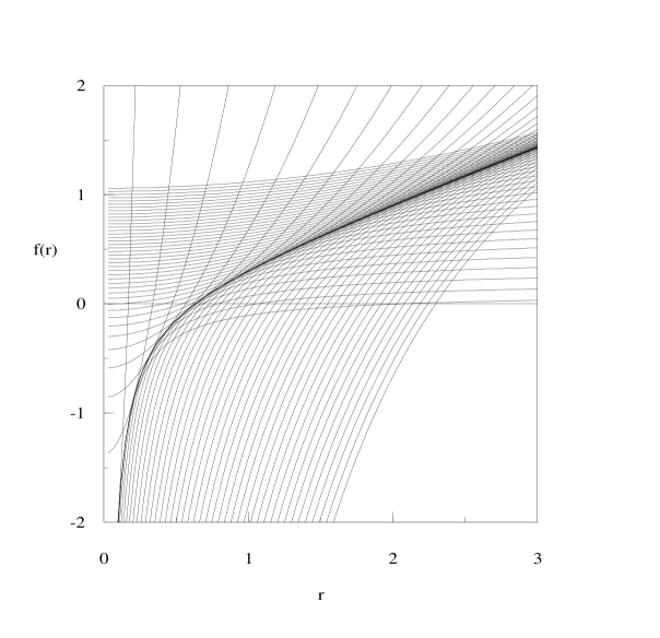
Figure 1: The “Coulomb-plus-linear” potential shape $f(r)=-a/r+br$ represented as the envelope curve of two distinct families of tangential potentials of the form $\alpha h(r)+\beta.$ In the upper family $h(r)=r^{2}$ is the harmonic-oscillator potential; in the lower family $h(r)=-1/r$ is the Coulomb potential. The adopted values of the relevant physical parameters $a$ and $b$ are $a=0.2$ and $b=0.5.$

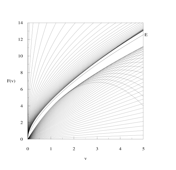
Figure 2: The spectral approximation corresponding to Fig. 1. Each “tangential” potential $f^{({\rm t})}(r)=\alpha h(r)+\beta$ generates a corresponding tangential energy curve $F^{({\rm t})}(v)=H(\alpha v)+\beta v.$ The envelopes of these spectral families generate upper and lower bounds to the exact curve $E=F(v),$ shown here for the case $(n,\ell)=(2,4).$

In the 1-term case the question arises as to whether there is a simple way of determining the envelopes of the families of upper and lower spectral functions. One effective solution of this problem is by the use of “kinetic potentials” which were introduced [12, 13] precisely for this purpose. The idea is as follows. To each spectral function $F_{n\ell}(v)$ there is a corresponding “kinetic potential” (that is, a minimum mean iso-kinetic potential) $\bar{f}_{n\ell}(s).$ The relationship between $F_{n\ell}$ and $\bar{f}_{n\ell}$ is invertible and is essentially that of a Legendre transformation [17]: we can prove in general that $F$ is concave, $\bar{f}(s)$ is convex, and

$$F^{\prime\prime}(v)\bar{f}^{\prime\prime}(s)=-\frac{1}{v^{3}}\ .$$

The explicit transformation formulas are as follows:

$$\bar{f}_{n\ell}(s)=F^{\prime}_{n\ell}(v)\ ,\quad s=F_{n\ell}(v)-vF^{\prime}_{n\ell}(v)$$ (7)

and

$$\frac{F_{n\ell}(v)}{v}=\bar{f}_{n\ell}(s)-s\bar{f}^{\prime}_{n\ell}(s)\ ,\quad\frac{1}{v}=-\bar{f}^{\prime}_{n\ell}(s)\ .$$ (8)

An a-priori definition of the ground-state kinetic potential $\bar{f}_{10}(s)=\bar{f}(s)$ is given by

$$\bar{f}(s)=\inf_{{{\scriptstyle\psi\in{\cal D}(H)}\atop{\scriptstyle(\psi,\psi)=1}}\atop{\scriptstyle(\psi,-\Delta\psi)=s}}(\psi,f\psi)\ ,$$

where ${\cal D}\subset L^{2}(\mbox{\vrule R}^{3})$ is the domain of the Hamiltonian. The definition for the excited states is a little more complicated [13] and, in view of (7) and (8), will not be needed in what follows.

What is crucial is that the spectral functions, either exact or approximate, are recovered from the corresponding kinetic potentials by a minimization over the kinetic-energy variable $s.$ In this way the total minimization required by the minimum–maximum principle [9, 11] has been divided into two steps: the first is constrained by $(\psi,-\Delta\psi)=s$ and the second is a minimization over $s.$ We have in all cases:

$$F_{n\ell}(v)=\min_{s>0}\left[s+v\bar{f}_{n\ell}(s)\right].$$

Another form of this expression is possible for the kinetic potential is monotone and allows us to change variables $(s\rightarrow r)$ by $f(r)=\bar{f}_{n\ell}(s).$ Thus we have

$$F_{n\ell}(v)=\min_{r>0}\left[K^{(f)}_{n\ell}(r)+vf(r)\right],\quad K^{(f)}_{n\ell}=\bar{f}_{n\ell}^{-1}\circ f\ .$$ (9)

The two corresponding expressions of the envelope approximation then become

$$\bar{f}_{n\ell}(s)\approx g(\bar{h}_{n\ell}(s))\ ,\quad{\rm or}\quad K^{(f)}_{n\ell}\approx K^{(h)}_{n\ell}\ .$$

The second form (9) of the explicit expression for $F_{n\ell}(v)$ isolates the potential shape $f$ itself and leads to an inversion sequence [18] which reconstructs the potential from a single given spectral function; but this is another story [19, 20].

It is useful here to provide the formulas for the kinetic potentials $\bar{f}$ corresponding to pure power-law potentials $V(r)=v\,{\rm sgn}(q)r^{q}.$ Elementary scaling arguments for the Hamiltonian

$$H=-\Delta+v\,{\rm sgn}(q)r^{q}$$

show that the eigenvalues satisfy

$$F_{n\ell}(v)=v^{\frac{2}{2+q}}F_{n\ell}(1)\ ,$$

where $F_{n\ell}(1)=E_{n\ell}(q)$ are the eigenvalues of $H$ with coupling $v=1,$ i.e., of $-\Delta+{\rm sgn}(q)r^{q}.$ From Eq. (7) we immediately find that the kinetic potentials $\bar{f}_{n\ell}(s)$ for these potentials $V(r)$ are given by

$$\bar{f}_{n\ell}(s)=\frac{2}{q}\left|\frac{qE_{n\ell}(q)}{2+q}\right|^{\frac{2+q}{2}}s^{-\frac{q}{2}}\ .$$ (10)

Meanwhile the corresponding $K$-functions all have the same simple form [21]

$$K_{n\ell}^{(q)}(r)=\left(\frac{P_{n\ell}(q)}{r}\right)^{2}\ ,$$

where the $P$ numbers are given by

$$P_{n\ell}(q)=\left|E_{n\ell}(q)\right|^{\frac{2+q}{2q}}\left(\frac{2}{2+q}\right)^{\frac{1}{q}}\left|\frac{q}{2+q}\right|^{\frac{1}{2}}\ ,\quad q\neq 0\ .$$

Consequently, the power-law kinetic potentials (10) may be expressed in the simple form

$$\bar{f}_{n\ell}(s)={\rm sgn}(q)\left(\frac{P_{n\ell}(q)}{\sqrt{s}}\right)^{q}\ ,\quad q\neq 0\ .$$

Some of the eigenvalues $E,$ and thus the corresponding $P$ numbers, are known exactly from elementary quantum mechanics. From the known eigenvalues $E$ for the Coulomb potential, $E_{n\ell}(-1)=-[2(n+\ell)]^{-2},$ and the harmonic-oscillator potential, $E_{n\ell}(2)=4n+2\ell-1,$ we immediately obtain the corresponding $P$ numbers:

$$P_{n\ell}(-1) = n+\ell\ ,$$

$$P_{n\ell}(2) = 2n+\ell-\frac{1}{2}\ .$$

The case $q=0$ corresponds exactly to the logarithmic potential [22, 23]; the $P$ numbers for the lowest states of the logarithmic and the linear potentials may be found in Table 1.

Table 1: Numerical values for the $P$ numbers for the logarithmic potential ($q=0$) and the linear potential ($q=1$) used in the Schrödinger eigenvalue formula (11).

$n$	$\ell$	$P_{n\ell}(0)$	$P_{n\ell}(1)$
1	0	1.21867	1.37608
2	0	2.72065	3.18131
3	0	4.23356	4.99255
4	0	5.74962	6.80514
5	0	7.26708	8.61823
1	1	2.21348	2.37192
2	1	3.68538	4.15501
3	1	5.17774	5.95300
4	1	6.67936	7.75701
5	1	8.18607	9.56408
1	2	3.21149	3.37018
2	2	4.66860	5.14135
3	2	6.14672	6.92911
4	2	7.63639	8.72515
5	2	9.13319	10.52596
1	3	4.21044	4.36923
2	3	5.65879	6.13298
3	3	7.12686	7.91304
4	3	8.60714	9.70236
5	3	10.09555	11.49748
1	4	5.20980	5.36863
2	4	6.65235	7.12732
3	4	8.11305	8.90148
4	4	9.58587	10.68521
5	4	11.06725	12.47532
1	5	6.20936	6.36822
2	5	7.64780	8.12324
3	5	9.10288	9.89276
4	5	10.56970	11.67183
5	5	12.04517	13.45756

In summary, if the potential $V(r)$ is a smooth transformation $V(r)=g({\rm sgn}(q)r^{q})$ of the pure power-law potential ${\rm sgn}(q)r^{q}$, then the eigenvalues of

$$H=-\Delta+V(r)$$

are given approximately by the expression

$$E_{n\ell}\approx\min_{r>0}\left[\frac{P_{n\ell}^{2}(q)}{r^{2}}+V(r)\right].$$ (11)

Here, a sign of approximate equality is used to indicate that, for a definite convexity of $g(h),$ Eq. (11) yields lower bounds for convex $g$ ($g^{\prime\prime}>0$) and upper bounds for concave $g$ ($g^{\prime\prime}<0$). The numbers $P_{n\ell}(q)$ can be derived from the eigenvalues of the operator $-\Delta+{\rm sgn}(q)r^{q}.$

The lower bounds derived in the framework of envelope theory can be improved by use of the refined comparison theorems of Ref. [24], which allow comparison potentials to intersect; a detailed study of the latter approach is, however, beyond the scope of the present analysis.

As an immediate application we consider the (nonrelativistic) Schrödinger Hamiltonian (6) for the semirelativistic spinless-Salpeter harmonic-oscillator problem (1). Here we have

$$H=-v\Delta+V(r)\ ,$$

with

$$V(r)=\beta\sqrt{m^{2}+r^{2}}\ ;$$

this potential is a convex transformation of a linear potential and a concave transformation of a harmonic-oscillator potential. We conclude therefore from Eq. (11) (see also Ref. [25]):

$$\min_{r>0}\left[v\frac{P_{n\ell}^{2}(1)}{r^{2}}+\beta\sqrt{m^{2}+r^{2}}\right]\leq{\cal E}_{n\ell}(v)\leq\min_{r>0}\left[v\frac{P_{n\ell}^{2}(2)}{r^{2}}+\beta\sqrt{m^{2}+r^{2}}\right],$$ (12)

where the numbers $P_{n\ell}(1)$ are given in Table 1 and $P_{n\ell}(2)=2n+\ell-\frac{1}{2}$. By a simple change of variables, $r\rightarrow r^{\prime}=P/r,$ we are able to recast the inequalities (12) into the “preferred” form

$${\cal E}_{n\ell}(v)\approx\min_{r>0}\left[\beta\sqrt{m^{2}+\frac{P^{2}_{n\ell}}{r^{2}}}+V(r)\right],\quad V(r)=vr^{2}\ ,$$

in which the function to be minimized is simply the spinless-Salpeter Hamiltonian with the momentum operator $|{\bf p}|$ replaced by $P/r;$ the $P$ numbers yielding upper and lower bounds are as in Eq. (12). Interestingly, the upper and lower bounds in Eq. (12) are equivalent to the corresponding bounds obtained in Ref. [8]; however, these earlier specific bounds were not derived as part of the general envelope theory. If we approximate the square root from above again, by using the elementary inequality

$$\sqrt{m^{2}+r^{2}}\leq m+\frac{r^{2}}{2m}\ ,$$

we obtain from (12) the weaker upper bound

$${\cal E}_{n\ell}(v)\leq\beta m+\sqrt{\frac{\beta v}{2m}}(4n+2\ell-1)\ ,$$

which is identical to that given by the general “Schrödinger upper bound” [26, 3, 4] obtained by initially approximating the relativistic kinetic-energy operator above by

$$\beta\sqrt{m^{2}+{\bf p}^{2}}\leq\beta\left(m+\frac{{\bf p}^{2}}{2m}\right).$$

The latter upper bound, and an improvement on it, will be discussed in the next section.

4 Envelope approximations for the relativistic kinetic energy

The relativistic kinetic-energy operator $T=\beta\sqrt{m^{2}+{\bf p}^{2}}$ is a concave transformation of ${\bf p}^{2}.$ Thus “tangent lines” to this operator all are of the form $a{\bf p}^{2}+b$ and each one generates a Schrödinger operator that provides an upper bound to $T.$ In a given application with given parameter values, one can search for the best such upper bound. By elementary analysis we can establish the operator inequality

$$H=\beta\sqrt{m^{2}+{\bf p}^{2}}+V(r)\leq\frac{\beta}{2}\left(-\frac{\Delta}{\mu}+\mu+\frac{m^{2}}{\mu}\right)+V(r)\ ,$$ (13)

where $\mu=\sqrt{m^{2}+p_{1}^{2}},$ and $|{\bf p}|=p_{1}$ is the “point of contact” of the tangent line with the square-root function. The inequality (13) is identical to that obtained [26] by employing the inequality $(T-\mu)^{2}\geq 0.$ Optimization over $\mu$ for the Coulomb case $V(r)=-v/r$ recovers the explicit upper-bound formula of Ref. [26]:

$$E_{n\ell}(v)\leq m\beta\sqrt{1-\left(\frac{v}{\beta(n+\ell)}\right)^{2}}\ .$$

In the case of the harmonic-oscillator potential, $V(r)=vr^{2},$ we obtain the upper bounds [8]

$$E_{n\ell}(v)\leq\min_{\mu>0}\left[\sqrt{\frac{\beta v}{2\mu}}(4n+2\ell-1)+\frac{\beta}{2}\left(\mu+\frac{m^{2}}{\mu}\right)\right].$$

(Brief reviews of analytical upper bounds on the energy eigenvalues of the spinless Salpeter equation derived by combining operator inequalities with the minimum–maximum principle may be found in Refs. [3, 4, 27].)

The strategy of the present section is to regard the relativistic kinetic-energy operator $T$ as a concave function of ${\bf p}^{2},$ so that “tangent lines” generate “upper” Schrödinger operators. This general approach leads to the same upper bounds as those of Martin [28] who used the particular square-root form of the relativistic kinetic energy to construct an operator whose positivity yields the bounds.

5 Envelope approximations for Salpeter Hamiltonians

5.1 The principal envelope formula

Let us now turn to our main topic and consider the spinless-Salpeter Hamiltonian of Eq. (1),

$$H=\beta\sqrt{m^{2}+{\bf p}^{2}}+V(r)\ ,$$

and its eigenvalues $E.$ We shall assume that the potential $V(r)$ is a smooth transformation $V(r)=g(h(r))$ of another potential $h(r)$ and that $g$ has definite convexity so that we obtain bounds to the energy eigenvalues $E$. We suppose that the “basis” potential $h(r)$ generates a “tangential” Salpeter problem

$${\cal H}=\beta\sqrt{m^{2}+{\bf p}^{2}}+vh(r)\ ,$$

for which the eigenvalues $e(v),$ or bounds to them, are known. We shall follow here as closely as possible the development in Sec. 3 for the corresponding Schrödinger problem.

First of all, we recall that the approximations or bounds to the energy eigenvalues of the relativistic Coulomb and harmonic-oscillator problems we shall eventually use from Secs. 2 and 3, when regarded as functions of the coupling $v,$ are all concave. Furthermore, it is easy to convince oneself that all the (unknown) energy functions $e(v)$ of the “tangential” Salpeter problem are concave, that is, $e^{\prime\prime}(v)<0.$ Suppose that the exact eigenvalue and (normalized) eigenvector for the problem posed by the “tangential” Hamiltonian

$${\cal H}=\beta\sqrt{m^{2}+{\bf p}^{2}}+vh(r)$$

are $e(v)$ and $\psi(v,r).$ Then, by differentiating the expectation value $(\psi,{\cal H}\psi)$ with respect to the coupling $v,$ we find

$$e^{\prime}(v)=(\psi,h\psi)\ .$$

If we now apply $\psi(v,r)$ as a trial vector to estimate the energy of the operator

$$\beta\sqrt{m^{2}+{\bf p}^{2}}+uh(r)\ ,$$

in which $v$ has been replaced by $u,$ we obtain an upper bound to the corresponding energy function $e(u)$ which may be written in the form

$$e(u)\leq e(v)+(u-v)e^{\prime}(v)\ .$$

This inequality tells us that the function $e(u)$ lies beneath its tangents; that is to say, $e(u)$ is concave. Convexity properties of the energy functions of the corresponding (nonrelativistic) Schrödinger problem have been investigated in Refs. [10, 12, 11].

Next, in order to prove the main result of this section, the “principal envelope formula,” we begin by using an envelope representation for the potential $V(r)$ in the Hamiltonian (1) and then demonstrate that all the spectral formulas that follow possess a certain structure. Finally, as an application, we specialize to the case of pure power-law “basis” potentials $h(r)$ and, more particularly, to the Coulomb potential and the harmonic-oscillator potential for which, at this time, we have spectral information [cf. the discussions in Secs. 2.2 and 2.3, and the exact bounds (12) on the energy levels ${\cal E}_{n\ell}(v)$ of the relativistic harmonic oscillator].

The tangential potentials we shall employ have the form $V^{({\rm t})}(r)=a(t)h(r)+b(t),$ where, as in the Schrödinger case, the coefficients $a(t)$ and $b(t)$ are given by

$$a(t)=\frac{V^{\prime}(t)}{h^{\prime}(t)}=g^{\prime}(h(t))\ ,\quad b(t)=V(t)-a(t)h(t)=g(h(t))-g^{\prime}(h(t))h(t)\ ,$$

and $r=t$ is the point of contact of the potential $V(r)$ and its tangent $V^{({\rm t})}(r)$. If, for the sake of definiteness, we assume that $V=g(h)$ with $g$ concave (i.e., $g^{\prime\prime}<0$), we obtain a family of upper bounds given by

$$E\leq\varepsilon(t)=e(a(t))+b(t)\ .$$

The best of these is given by optimizing over $t$:

$$E\leq\varepsilon(\hat{t})=e(a(\hat{t}))+b(\hat{t})\ ,$$

where $\hat{t},$ the value of $t$ which optimizes these bounds, is to be determined as the solution of

$$e^{\prime}(g^{\prime}(h(\hat{t})))=h(\hat{t})\ .$$

In the spirit of the Legendre transformation [17] we now consider another problem which has the same solution; this second problem is the one that provides us with our basic eigenvalue formula. We consider

$${\cal E}\equiv\min_{v>0}[e(v)-ve^{\prime}(v)+g(e^{\prime}(v))]\ ,$$

which is well defined since $e(v)$ is concave. The solution has the critical point

$$\hat{v}=g^{\prime}(e^{\prime}(\hat{v}))\ .$$

If we now apply the correspondence $h(\hat{t})=e^{\prime}(\hat{v}),$ it follows that the critical point $\hat{v}$ becomes

$$\hat{v}=g^{\prime}(h(\hat{t}))\ ,$$

and the tangential-potential coefficients $a$ and $b$ become

$$a(\hat{t})=g^{\prime}(e^{\prime}(v))=v\ ,\quad b(\hat{t})=g(e^{\prime}(v))-ve^{\prime}(v)\ ,\quad v=\hat{v}\ .$$ (14)

Meanwhile the original critical (energy) value is given by

$$\varepsilon(\hat{t})=e(a(\hat{t}))+b(\hat{t})=e(v)-ve^{\prime}(v)+g(e^{\prime}(v))\ ,\quad v=\hat{v}\ .$$

Thus we conclude that the spectral approximation obtained by envelope methods is given by the following “principal envelope formula:”

$$E\approx{\cal E}\equiv\min_{v>0}[e(v)-ve^{\prime}(v)+g(e^{\prime}(v))]\ .$$ (15)

If $g$ is concave (that is, $g^{\prime\prime}<0$), then $E\leq{\cal E};$ if $g$ is convex (that is, $g^{\prime\prime}>0$), then $E\geq{\cal E}.$ From the above considerations it follows immediately that, if the exact energy function $e(v)$ corresponding to the basis potential $h$ is not available, then, for $g(h)$ concave, concave upper approximations $e_{\rm u}(v)>e(v)$ or, for $g(h)$ convex, concave lower approximations $e_{\rm l}(v)<e(v)$ may be used instead of the exact energy function $e(v)$ in the principal envelope formula (15). Then all the lower tangents will lie even lower and all the upper tangents will lie even higher. If $g$ is convex, we obtain a lower bound; if $g$ is concave, we obtain an upper bound; because of the concavity of $e(v),$ this extremum is a minimum in both cases. If we wish to use numerical solutions to the “basis” problem (generated by $h(r)$), or if a completely new energy-bound expression becomes available, the principal envelope formula (15) is the relation that would at first be used.

Interestingly, in the formula (15) the tangential-potential apparatus is no longer evident; only the correct convexity is required. As in the Schrödinger case [12], once we have the basic result, the reformulation in terms of “kinetic potentials” is often useful: the kinetic potential $\bar{h}(s)$ corresponding to some basis potential $h(r)$ is given by the Legendre transformation [17]

$$\bar{h}(s)=e^{\prime}(v)\ ,\quad s=e(v)-ve^{\prime}(v)\ .$$

Meanwhile the envelope approximation has the kinetic-potential expression $\bar{V}(s)\approx g(\bar{h}(s)).$

For both the Coulomb lower bounds (3) or (5) and the harmonic-oscillator upper bounds (12) which we have at present, we may express our general results in a special common form which will now be derived.

5.2 The Coulomb lower bound

We consider first the Coulomb lower bound in which we assume that the potential $V(r)$ is a convex transformation $V(r)=g(h(r))$ of the Coulomb potential $h(r)=-1/r.$ According to Sec. 2.2, in this case all the “lower” $e_{\rm l}(v)$ have been arranged—with the parameters $\beta$ and $m$ returned—in the form

$$e_{\rm l}(v)=\beta m\sqrt{1-\left(\frac{\sigma v}{\beta}\right)^{2}}\ .$$

From this it follows by elementary algebra that if we define a new optimization variable $r$ by $e_{\rm l}^{\prime}(v)=h(r)=-1/r,$ we have

$$e_{\rm l}(v)-ve_{\rm l}^{\prime}(v)=\beta\sqrt{m^{2}+\frac{P^{2}}{r^{2}}}\ ,\quad P\equiv\frac{1}{\sigma}\ .$$

Consequently, the lower bound on the energy eigenvalues $E$ of the spinless Salpeter equation becomes

$$E\geq\min_{r>0}\left[\beta\sqrt{m^{2}+\frac{P^{2}}{r^{2}}}+V(r)\right],\quad v<\beta v_{P}\ .$$ (16)

Here the boundary value $v_{P}$ of the Coulomb coupling $v$ is given, when simply determined by the requirement of boundedness from below of the operator (1), by the critical coupling $v_{\rm c}$,

$$v_{P}=v_{\rm c}=\frac{2}{\pi}\ ,$$

and, when arising from the region of validity of our Coulomb-like family of lower bounds (5), via $P=1/\sigma,$ by

$$v_{P}=P\sqrt{1-P^{2}}<\frac{1}{2}\ .$$ (17)

Some $\{P,v_{P}\}$ pairs may be found in Table 2; others can be easily generated from the upper bound on the coupling $v$ given in Eq. (17). The meaning of the Coulomb-coupling constraint is $a(\hat{t})<\beta v_{P},$ where $a$ is the coefficient in the tangential Coulomb potential given by (14).

Table 2: Explicit values of some $\{P,v_{P}\}$ pairs, obtained via the equality $P=1/\sigma$ either from the Herbst lower bound (3) or the expression (5) for our new lower bounds on the spectrum of the spinless relativistic Coulomb problem (in three spatial dimensions).

$P$	$v_{P}$
$\displaystyle\frac{2}{\pi}$	$\displaystyle\frac{2}{\pi}$
$\displaystyle\frac{1}{\sqrt{2}}$	$\displaystyle\frac{1}{2}$
$\sqrt{\displaystyle\frac{2}{9-3\sqrt{5}}}$	$\displaystyle\frac{1}{3}$
$\displaystyle\frac{1}{2\sqrt{2-\sqrt{3}}}$	$\displaystyle\frac{1}{4}$

As a rather trivial consistency check of our formalism, the Coulomb lower energy bound of Eq. (16) may be applied to the Coulomb potential $V(r)=-v/r$ in order to re-derive, for $P=2/\pi,$ the Herbst formula (3)—which is nothing else but the starting point of the present “lower-bound” considerations.

5.3 The harmonic-oscillator upper bounds

Next, let us turn to the harmonic-oscillator upper bounds. Our main assumption is here that $V(r)=g(r^{2}),$ with $g^{\prime\prime}<0.$ In this case the only difficulty is that the basis problem $h(r)=r^{2}$ is equivalent to a Schrödinger problem whose solution ${\cal E}_{n\ell}(v)$ is not known exactly. Following the discussion of suitable bounds after the proof of the principal envelope formula, Eq. (15), let us call the upper bound provided by Eq. (12) $e_{\rm u}(v),$ and let us introduce the shorthand notation $P_{n\ell}(2)=2n+\ell-\frac{1}{2}=P.$ Then we have the following parametric equations for $e_{\rm u}(v)$:

$$e_{\rm u}(v)=v\frac{P^{2}}{r^{2}}+\beta\sqrt{m^{2}+r^{2}}\ ,\quad v=\frac{\beta r^{4}}{2P^{2}\sqrt{m^{2}+r^{2}}}\ ,\quad e_{\rm u}^{\prime}(v)=\frac{P^{2}}{r^{2}}\ .$$

By substituting these expressions into the fundamental envelope formula (15) we obtain the following upper bound on all the eigenvalues of the spinless-Salpeter problem with potential $V(r)=g(r^{2})$ and $g^{\prime\prime}<0$:

$$E_{n\ell}\leq\min_{r>0}\left[\beta\sqrt{m^{2}+\frac{P^{2}}{r^{2}}}+V(r)\right],\quad P=P_{n\ell}(2)=2n+\ell-\frac{1}{2}\ .$$ (18)

6 The Coulomb-plus-linear (or “funnel”) potential

In order to illustrate the above results by a physically motivated example, let us apply these considerations to the Coulomb-plus-linear or (in view of its shape) “funnel” potential

$$V(r)=-\frac{c_{1}}{r}+c_{2}r\ ,\quad c_{1}\geq 0\ ,\quad c_{2}\geq 0\ .$$

(This potential provides a reasonable overall description of the strong interactions of quarks in hadrons. For the phenomenological description of hadrons in terms of both nonrelativistic and semirelativistic potential models, see, e.g., Refs. [29, 30].) By choosing as basis potential the Coulomb potential $h(r)=-1/r,$ we may write $V(r)=g(h(r))$ with

$$g(h)=c_{1}h-\frac{c_{2}}{h}\ ,$$

which is clearly a convex function of $h<0$: $g^{\prime\prime}>0.$ Thus the convexity condition is satisfied. However, we are not free to choose the coupling constants $c_{1}$ and $c_{2}$ as large as we please. It is immediately obvious that, for a particular $\{P,v_{P}\}$ pair, we must in any case have $c_{1}<\beta v_{P}.$ For the full problem the coefficient $c_{2}$ of the linear term will also be involved. The coupling $v$ we are concerned about is given by (14). We have

$$v=g^{\prime}(e^{\prime}(v))=\frac{\beta P^{2}}{r\sqrt{m^{2}+\left(\displaystyle\frac{P}{r}\right)^{2}}}=c_{1}+\frac{c_{2}}{h^{2}}=c_{1}+c_{2}r^{2}\ .$$

From this we obtain, for given values of the parameters $m$ and $\beta$ and for a given $\{P,v_{P}\}$ pair, as a sufficient condition for $v<\beta v_{P}$ the “Coulomb coupling constant constraint” on the two coupling strengths $c_{1}$ and $c_{2}$ in the funnel potential:

$$c_{1}+\frac{P^{2}}{m^{2}}\left(\frac{P^{2}}{v_{P}^{2}}-1\right)c_{2}<\beta v_{P}\ .$$ (19)

In the case $\{P=1/\sqrt{2},v_{P}=1/2\}$ and $\beta=m=1$ this condition reduces to $c_{1}+\frac{1}{2}c_{2}<\frac{1}{2}.$ For Herbst’s lower bound (3), i.e., $P=v_{P}=v_{\rm c}=2/\pi,$ this constraint clearly yields $c_{1}<\beta v_{P}.$ There is no escaping this feature of all energy bounds involving the Coulomb potential: the constraint derives from the fundamental observation that the Coulomb coupling $v$ must not be too large, so that the (relativistic) kinetic energy is able to counterbalance the Coulomb potential in order to maintain the Hamiltonian (1) with $V(r)=-v/r$ bounded from below.

For example, if we seek the largest allowed value of the parameter $P$ by solving Eqs. (17) and (19) together, we find that this largest $P$ is given by

$$\frac{c_{2}\sin^{4}t}{\cos^{2}t(\beta\sin t\cos t-c_{1})}=m^{2}\ ,\quad P\equiv\sin t\ .$$ (20)

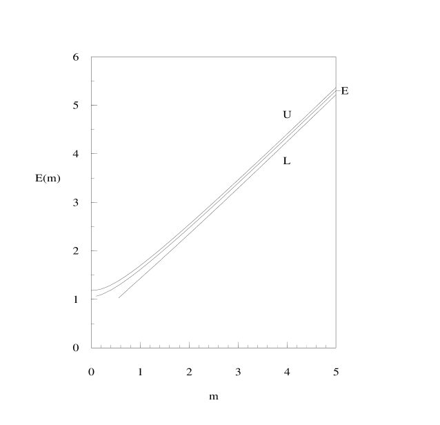
Figure 3: Lower bounds (L), according to (16), and upper bounds (U), according to (18), on the energy eigenvalue $E$ of the ground state [$(n,\ell)=(1,0)$] of the spinless Salpeter equation with a Coulomb-plus-linear potential $V(r)=-c_{1}/r+c_{2}r,$ for $\beta=1,$ $c_{1}=0.1,$ and $c_{2}=0.25.$ The lower bound is given by the general result (16) with the “best” $P(m)$ provided by (20). In order to satisfy the Coulomb coupling constraint (20), the mass $m$ must fulfil $m>\sqrt{5}/4.$ For comparison, a (very accurate) Rayleigh–Ritz variational upper bound $E$ is depicted too.

For the Coulomb-plus-linear potential $V(r)=-c_{1}/r+c_{2}r$ under consideration, Fig. 3 shows the lower and upper bounds on the lowest energy eigenvalue $E$ of the spinless Salpeter equation, given by the envelopes of the lower and upper families of tangential energy curves (16) and (18), as functions $E(m)$ of the mass $m$ entering in the semirelativistic Hamiltonian. In the case of the Coulomb lower bound (16), we have employed for each $m$ the best possible $P(m)$ provided by (20). As $m\to 0,$ the “basis” Coulomb problem $H=\beta\sqrt{m^{2}+{\bf p}^{2}}-v/r$ has energy $e(m)\to 0;$ thus the Coulomb lower bound for a non-Coulomb problem becomes very weak for small values of $m.$ Of course, Eq. (18) provides us with rigorous upper bounds for every energy level.

In order to get an idea of the location of the exact energy eigenvalues $E$, Fig. 3 also shows the ground-state energy curve $E(m)$ obtained by the Rayleigh–Ritz variational technique [9] with the Laguerre basis states for the trial space defined in Ref. [31]. Strictly speaking, this energy curve represents only an upper bound to the precise eigenvalue $E$. However, from the findings of Ref. [31] the deviations of these Laguerre bounds from the exact eigenvalues may be estimated, for the superposition of 25 basis functions used here, to be of the order of 1 %.

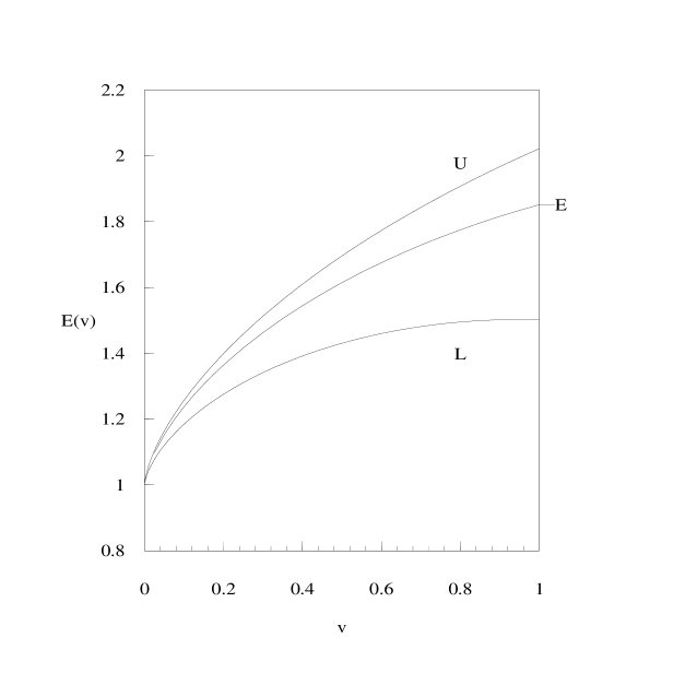
Figure 4: Lower bounds (L), according to (16), and upper bounds (U), according to (18), on the energy eigenvalue $E$ of the ground state [$(n,\ell)=(1,0)$] of the spinless Salpeter equation with Coulomb-plus-linear potential $V(r)=v(-a/r+br),$ for $a=0.2,$ $b=0.5,$ $m=\beta=1.$ The lower bound is given by the general result (16) with $P(m=1)$ computed from Eq. (20), evaluated for mass $m=1$ and the funnel-potential coupling strengths $c_{1}=va$ and $c_{2}=vb.$ For comparison, a (very accurate) Rayleigh–Ritz variational upper bound $E$ is depicted too.

Figure 4 shows, for a Coulomb-plus-linear potential of the form $V(r)=v(-a/r+br),$ the lower and upper bounds on the lowest energy eigenvalue $E$ of the spinless Salpeter equation, given by the envelopes of the lower and upper families of tangential energy curves (16) and (18), as functions $E(v)$ of the “overall” coupling parameter $v$ which multiplies the potential shape $-a/r+br.$ Again we compare these bounds with the ground-state energy curve $E(v),$ obtained by the Rayleigh–Ritz variational technique [9] with the Laguerre basis states [31].

7 Summary and conclusion

In this analysis we have studied the discrete spectrum of semirelativistic “spinless-Salpeter” Hamiltonians $H,$ defined in Eq. (1), by an approach which is based principally on convexity. We have at our disposal very definite information concerning, on the one hand, the bottom of the spectrum of $H$ for the Coulomb potential, $h(r)=-1/r,$ and, on the other hand, the entire spectrum of $H$ for the harmonic-oscillator potential, $h(r)=r^{2}.$ The class of potentials that are at the same time a convex transformation of $-1/r$ and a concave transformation of $r^{2}$ includes, for example, arbitrary linear combinations of Coulomb, logarithmic, linear, and harmonic-oscillator terms. In order to obtain information about the eigenvalues $E$ of $H$ for arbitrary members within this class of potentials, we have extended the—for nonrelativistic Schrödinger operators well-established—formalism of envelope theory to Hamiltonians with relativistic kinetic energies. The envelope technique applied here takes advantage of the fact that all “tangent lines” to the interaction potential $V(r)=g(h(r))$ in $H$ are potentials of the form $ah(r)+b,$ and that, by convexity and the comparison theorem recalled in Subsec. 2.4, the energy eigenvalues corresponding to these “tangent” potentials provide rigorous bounds to the unknown exact eigenvalues $E$ of $H.$ If $e(v)$ denotes the energy function—or a suitable bound to it—corresponding to the problem posed by a “basis” potential $vh(r),$ where $v$ is a positive coupling parameter, the envelopes of upper and lower families of energy curves may be found with the help of the “principal envelope formula”

$$E\approx\min_{v>0}[e(v)-ve^{\prime}(v)+g(e^{\prime}(v))]\ .$$

Here, a sign of approximate equality is used to indicate that, for a definite convexity of $g(h),$ the envelope theory yields lower bounds for convex $g(h)$ and upper bounds for concave $g(h).$ With the above principal envelope formula at hand, all new spectral pairs $\{h(r),e(v)\}$ which may become available at some future time can immediately be used to enrich our collection of energy bounds. If the basis potential $h(r)$ is a pure power, these bounds can be written as

$$E_{n\ell}\approx\min_{r>0}\left[\beta\sqrt{m^{2}+\frac{P_{n\ell}^{2}}{r^{2}}}+V(r)\right],$$

where the numbers $P_{n\ell}$ are obtained from the corresponding underlying basis problems. The power of this technique is illustrated, in Sec. 6, by our application to the “funnel” potential, $V(r)=-c_{1}/r+c_{2}r.$ For this problem, we have employed both the semirelativistic Coulomb and harmonic-oscillator problems to calculate, respectively, lower and upper bounds on the energy eigenvalues of the spinless Salpeter equation.

We expect that such results would provide bounds on the energy eigenvalues for general theoretical discussions, or be used as guides for more tightly focussed analytic or numerical studies of the spectra of semirelativistic “spinless-Salpeter” Hamiltonians.

References

- [1] E. E. Salpeter and H. A. Bethe, Phys. Rev. 84, 1232 (1951).
- [2] E. E. Salpeter, Phys. Rev. 87, 328 (1952).
- [3] W. Lucha and F. F. Schöberl, Int. J. Mod. Phys. A 14, 2309 (1999), hep-ph/9812368.
- [4] W. Lucha and F. F. Schöberl, Fizika B 8, 193 (1999), hep-ph/9812526.
- [5] I. W. Herbst, Commun. Math. Phys. 53, 285 (1977); 55, 316 (1977) (addendum).
- [6] A. Martin and S. M. Roy, Phys. Lett. B 233, 407 (1989).
- [7] W. Lucha and F. F. Schöberl, Phys. Rev. A 60, 5091 (1999), hep-ph/9904391.
- [8] W. Lucha and F. F. Schöberl, Int. J. Mod. Phys. A 15, 3221 (2000), hep-ph/9909451.
- [9] M. Reed and B. Simon, Methods of Modern Mathematical Physics IV: Analysis of Operators (Academic Press, New York, 1978).
- [10] H. Narnhofer and W. Thirring, Acta Phys. Austriaca 41, 281 (1975).
- [11] W. Thirring, A Course in Mathematical Physics 3: Quantum Mechanics of Atoms and Molecules (Springer, New York/Wien, 1990).
- [12] R. L. Hall, J. Math. Phys. 24, 324 (1983).
- [13] R. L. Hall, J. Math. Phys. 25, 2708 (1984).
- [14] R. L. Hall and N. Saad, J. Chem. Phys. 109, 2983 (1998).
- [15] R. L. Hall, J. Phys. A 19, 2079 (1986).
- [16] R. L. Hall, Phys. Rev. Lett. 83, 468 (1999).
- [17] I. M. Gelfand and S. V. Fomin, Calculus of Variations (Prentice-Hall, Englewood Cliffs, 1963). Legendre transformations are discussed on p. 72.
- [18] R. L. Hall, Phys. Lett. A 265, 28 (2000).
- [19] R. L. Hall, J. Phys. A 28, 1771 (1995).
- [20] R. L. Hall, J. Math. Phys. 40, 699 (1999).
- [21] R. L. Hall, J. Math. Phys. 34, 2779 (1993).
- [22] C. Quigg and J. L. Rosner, Phys. Rep. 56, 167 (1979).
- [23] R. L. Hall, J. Phys. G 26, 981 (2000); ESI programme Confinement (Vienna, Austria, 2000).
- [24] R. L. Hall, J. Phys. A 25, 4459 (1992).
- [25] R. L. Hall, W. Lucha, and F. F. Schöberl, J. Phys. A 34, 5059 (2001), hep-th/0012127.
- [26] W. Lucha and F. F. Schöberl, Phys. Rev. A 54, 3790 (1996), hep-ph/9603429.
- [27] W. Lucha and F. F. Schöberl, in: Proceedings of the XIth International Conference “Problems of Quantum Field Theory,” edited by B. M. Barbashov, G. V. Efimov, and A. V. Efremov, July 13 – 17, 1998, Dubna, Russia (Joint Institute for Nuclear Research, Dubna, 1999), p. 482, hep-ph/9807342.
- [28] A. Martin, Phys. Lett. B 214, 561 (1988).
- [29] W. Lucha, F. F. Schöberl, and D. Gromes, Phys. Rep. 200, 127 (1991).
- [30] W. Lucha and F. F. Schöberl, Int. J. Mod. Phys. A 7, 6431 (1992).
- [31] W. Lucha and F. F. Schöberl, Phys. Rev. A 56, 139 (1997), hep-ph/9609322.