Reflection Amplitudes of Boundary Toda Theories

and Thermodynamic Bethe Ansatz

Changrim Ahn¹, Chanju Kim² and Chaiho Rim³

¹Department of Physics, Ewha Womans University

Seoul 120-750, Korea

² Department of Physics and Center for Theoretical Physics, Seoul National University

Seoul 151-747, Korea

³ Department of Physics, Chonbuk National University

Chonju 561-756, Korea

PACS: 11.25.Hf, 11.55.Ds

Abstract

We study the ultraviolet asymptotics in $A_{n}$ affine Toda theories with integrable boundary actions. The reflection amplitudes of non-affine Toda theories in the presence of conformal boundary actions have been obtained from the quantum mechanical reflections of the wave functional in the Weyl chamber and used for the quantization conditions and ground-state energies. We compare these results with the thermodynamic Bethe ansatz derived from both the bulk and (conjectured) boundary scattering amplitudes. The two independent approaches match very well and provide the non-perturbative checks of the boundary scattering amplitudes for Neumann and $(+)$ boundary conditions. Our results also confirm the conjectured boundary vacuum energies and the duality conjecture between the two boundary conditions.

1 Introduction

A large class of massive 2D integrable quantum field theories (IQFTs) can be considered as perturbed conformal field theories (CFTs) [1]. The ultraviolet (UV) behavior of these IQFTs is encoded in the CFT data while their long distance properties are defined by the S-matrix data. If the basic CFT admits the representation of the primary fields of full symmetry algebra in terms of the exponential fields, the CFT data include “reflection amplitudes”. These functions define the linear transformations between different exponential fields, corresponding to the same primary field. Reflection amplitudes play a crucial role for the calculation of the one-point functions [2] as well as for the description of the zero-mode dynamics [3, 4, 5] in integrable perturbed CFTs. In particular, the zero-mode dynamics determines the UV asymptotics of the ground state energy $E(R)$ (or effective central charge $c_{\rm eff}(R)$) for the system on the circle of size $R$. The function $c_{\rm eff}(R)$ admits in this case the UV series expansion in the inverse powers of $\log(1/R)$. The solution of the quantization condition for the vacuum wave function (which can be written in terms of the reflection amplitudes), supplemented with the exact relations between the parameters of the action and the masses of the particles determines all logarithmic terms in this UV expansion.

The effective central charge $c_{\rm eff}(R)$ in IQFT can be also calculated independently from the S-matrix data using the TBA method [6]. At small $R$ its asymptotics can be compared with that following from the CFT data. In the case when the basic CFT is known the agreement of both approaches can be considered as nontrivial test for the S-matrix amplitudes in IQFT. The corresponding analysis based on the both approaches was previously done for the sinh-Gordon [3], supersymmetric sinh-Gordon, Bullough-Dodd [4] models, simply-laced affine Toda field theories (ATFTs) [5] and nonsimply-laced ATFTs [7].

In this paper we extend this method to the ATFTs with integrable boundary actions. IQFTs with the integrable boundary actions can also be interpreted as boundary CFTs perturbed by both bulk and boundary operators [8]. The boundary ATFTs are the non-affine Toda theories (NATTs) with boundary perturbed by both bulk and boundary operators associated with the affine roots. These models become increasingly interesting due to their potential applicability to condensed matter systems. For IQFTs with boundary, a new physical quantity called “boundary $S$-matrix” satisfies the boundary Yang-Baxter equations and associated bootstrap equations. These equations determine the boundary $S$-matrices upto CDD-like factors and most cases are without direct relations with the boundary actions. It is an important issue to relate these two informations. Differently from the bulk, even perturbative checks for the boundary $S$-matrices are very complicated because of the half-line geometry. One of our main results in this paper is to provide such non-perturbative confirmation of the proposed boundary $S$-matrices of the $A_{n}$ ATFTs.

For this purpose, we work out the boundary version of the TBA equations for these models to obtain the ground state energy. The effects of the boundary $S$-matrices are encoded into the fugacity of the TBA equations. To describe the zero-mode dynamics, we obtain the “boundary reflection amplitudes” of the NATTs by considering reflections of the wave functional inside the Weyl chamber. Our results are exactly the same as those obtained by functional relations in [9]. The quantization conditions and effective central charges of the ATFTs can be obtained from these reflection amplitudes. We show that these two independent results match upto high accuracy for $A_{n}$ ATFTs and corresponding boundary actions. While our analysis is valid in the UV region, it is noticed that two results agree well even upto $R\sim{\cal O}(1)$ if exact vacuum energies are considered. There are two contributions to the vacuum energies, one from the bulk term which is proportional to $R^{2}$ and the other from the boundary term proportional to $R$. Both contributions become significant as $R$ increases. Accurate agreement upto this scale provides nonperturbative check of the boundary vacuum energies conjectured in [9].

The rest of the paper is organized as follows. In sect.2 we introduce the simply-laced ATFTs with integrable boundary actions along with the boundary TBA equations based on the bulk and boundary $S$-matrices corresponding to the Neumann and $(+)$ boundary conditions (see below). In sect.3 we consider $A_{1}$ NATT, namely the Liouville field theory (LFT) with boundary, and estabilish the wave functional description in terms of the boundary reflection amplitude of the LFT with boundary. Using this result, we derive the boundary reflection amplitudes for the simply-laced NATTs. In sect.4 we analyze the quantization conditions and UV asymptoics of ground state energies and effective central charges. We follow closely the cases without boundary considered in [5]. Comparison of these results with numerical solutions of the TBA equations and with the vacuum energies are presented in sect.5. We conclude in sect.6 with open questions and some remarks.

2 Affine Toda Theories on a half line

2.1 Integrable Actions, Bulk and Boundary $S$-Matrices

The ATFTs corresponding to Lie algebra $G$ is described by the action

$${\cal A}=\int d^{2}x\left[{1\over{8\pi}}(\partial_{a}\boldsymbol{\varphi})^{2}+\mu\sum_{i=0}^{r}e^{b{\bf e}_{i}\cdot\boldsymbol{\varphi}}\right]+\mu_{B}\int dx\sum_{i=0}^{r}\eta_{i}e^{b{\bf e}_{i}\cdot\boldsymbol{\varphi}/2},$$ (1)

where ${\bf e}_{i},\ i=1,\ldots,r$ are the simple roots of the Lie algebra $G$ of rank $r$ and $-{\bf e}_{0}$ is a maximal root satisfying

$${\bf e}_{0}+\sum_{i=1}^{r}n_{i}{\bf e}_{i}=0.$$ (2)

For real $b$ the spectrum of these ATFTs consists of $r$ particles with the masses $m_{i}$ ($i=1,\ldots,r$) given by

$$m_{i}={\overline{m}}\nu_{i}$$ (3)

where

$${\overline{m}}^{2}={1\over{2h}}\sum_{i=1}^{r}m_{i}^{2}$$ (4)

and here $h$ is Coxeter number and $\nu_{i}^{2}$ are the eigenvalues of the mass matrix:

$$M_{ab}=\sum_{i=0}^{r}({\bf e}_{i})^{a}({\bf e}_{i})^{b}.$$ (5)

The mass-$\mu$ relation is

$$-\pi\mu\gamma(1+b^{2})=\left[{{\overline{m}}k(G)\Gamma\left({1\over{(1+b^{2})h}}\right)\Gamma\left(1+{b^{2}\over{(1+b^{2})h}}\right)\over{2\Gamma(1/h)}}\right]^{2(1+b^{2})}$$ (6)

where $\gamma(x)=\Gamma(x)/\Gamma(1-x)$ and

$$k(G)=\left(\prod_{i=1}^{r}n_{i}^{n_{i}}\right)^{1/2h}$$ (7)

with $n_{i}$ defined in Eq.(2).

The scattering amplitudes of the ATFTs are factorized into the two-particle bulk $S$-matrices. From the bootstrap relations, crossing symmetry, and unitarity, the $S$-matrix between the particles $m_{i}$ and $m_{j}$ are given by [10, 11]:

$$S_{ij}(\theta) = \exp(-i\delta_{ij}(\theta))\qquad{\rm where}$$ (8)

$$\delta_{ij}(\theta) = \int_{0}^{\infty}{dt\over{t}}\left[8\sinh\left({\pi Bt\over{h}}\right)\sinh\left({\pi(1-B)t\over{h}}\right){\left(2\cosh{\pi t\over{h}}-{\bf I}\right)^{-1}}_{ij}-2\delta_{ij}\right]\sin(\theta t),$$

where ${\bf I}$ is the incident matrix defined by ${\bf I}_{ij}=2\delta_{ij}-{\bf e}_{i}\cdot{\bf e}_{j}$ and with

$$B={b^{2}\over{1+b^{2}}}.$$ (9)

The second term in (1) is the boundary action which preserves the integrability. The boundary parameter $\mu_{B}$ should be fixed completely to have conserved charges [12, 13]

$$\mu_{B}^{2}={\mu\over{2}}\cot\left({\pi b^{2}\over{2}}\right)$$ (10)

with discrete parameter

$$\eta_{i}=1,\quad-1,\quad 0.$$ (11)

Only exception is the $A_{1}$-ATFT, namely the sinh-Gordon model, which include two continuous free parameters on boundary. These extra parameters introduce additional complicacy in the analysis [14] and will not be considered here.

With the integrable boundary actions, the boundary $S$-matrices should satisfy the boundary Yang-Baxter equations and boundary bootstrap relations [15, 16] along with boundary crossing-unitarity relation [8]. With diagonal bulk $S$-matrices of the ATFTs, these relations can determine the boundary $S$-matrices only upto CDD factors. This CDD ambiguity is more serious for the IQFTs with boundary. While the bulk $S$-matrices can be checked both perturbatively and nonperturbatively, the boundary $S$-matrices is difficult to check perturbatively due to the presence of boundary [17], not to mention non-perturbative checks. In addition, there is no clear relations between the boundary actions and specific CDD factors to be chosen. So far, only a few boundary $S$-matrices have been associated with combinations of the discrete possibilities Eq.(11). In this paper we will consider only the simplest case where all the parameters $\eta_{i}=+1$ denoted by $(+)$ boundary condition (BC) and the Neumann (free) BC denoted by $(f)$ with all $\eta_{i}=0$, which is conjectured to be a dual ($b\to 1/b$) of $(+)$ [18]. We will impose the two BCs $(+)$ and $(f)$ independently on both boundaries of the strip. These are the cases without boundary bound states where the standard “ground state” TBA should work.

For $A_{n-1}^{(1)}$ ATFTs, the boundary $S$-matrices $R_{j}(\theta)$ for the $(+)$ BCs are given by [12]

$$R^{(+)}_{j}(b,\theta)=\prod_{a=1}^{j}[a-1][a-n][-a+B][-a-n+1-B],\quad j=1,\ldots,n-1$$ (12)

where

$$[x]={\sinh(\theta/2+i\pi x/2h)\over{\sinh(\theta/2-i\pi x/2h)}}.$$ (13)

The boundary $S$-matrices for the free BCs are conjectured to be dual transform of the $(+)$ BCs, namely,

$$R^{(f)}_{j}(b,\theta)=R^{(+)}_{j}(1/b,\theta).$$ (14)

We will consider only the $A$-type ATFTs to avoid extra complicacy arising from ambiguous CDD factors for $D$- and $E$-type ATFTs.

2.2 Boundary TBA

TBA equations are constructed in the rectangle with each size $R$ and $L$. The free energy given by scattering theories defined on the space with infinite size $L$ and imaginary time $R=1/T$ (“$R$-channel”) is compared with the opposite case where the Casimir energy $E_{0}(R)$ is obtained as a function of finite spatial size $R$ while the time $L$ (“$L$-channel”) goes to $\infty$. With periodic BCs, the opposite case of $L$ finite and $R\to\infty$ does not raise any new problem since it is identical to the above by just interchanging $R$ and $L$.

In the presence of boundaries where specific integrable BCs are imposed, these two cases have totally different meanings because one of the size, say $R$, should denote the width between two sides where the BCs are imposed [19]. Now consider the former case. In the $R$-channel, the thermodynamic functions are defined by the scattering theories with “fugacity” where the boundary states act as creating/annihilating sources of particle pairs with certain probabilities which are determined by the boundary $S$-matrices. The physical quantity generated by the TBA is the Casimir energy $E_{0}^{\alpha\beta}(R)$ which depends on the specific BCs $(\alpha)$ and $(\beta)$. The Casimir energy is related to the effective central charges of the underlying CFTs. In opposite case of $R\to\infty$, the thermodynamic analysis generates the boundary entropy instead.

For the irrational CFTs like the NATTs, it is quite difficult to define conformal boundary states and associated boundary entropies. Therefore, we will concentrate on the former case of $L\to\infty$ with finite $R$ in which the boundary TBA generates the effective central charge.

Following the the formalism of [19], we can derive the TBA equations straightforwardly because the boundary ATFTs are purely diagonal scattering theories. The TBA equations for the ATFTs are given by ($i=1,\cdots,r$)

$$2m_{i}R\cosh\theta=\epsilon_{i}(\theta)+\sum_{j=1}^{r}\int_{-\infty}^{\infty}\varphi_{ij}(\theta-\theta^{\prime})\log\left(1+\lambda^{(\alpha\beta)}_{i}(\theta^{\prime})e^{-\epsilon_{i}(\theta^{\prime})}\right){d\theta^{\prime}\over 2\pi},$$ (15)

where $\varphi_{ij}$ is the kernel which is equal to the logarithmic derivative of the $S$-matrix $S_{ij}(\theta)$ in Eq.(8)

$$\varphi_{ij}(\theta)=-i{d\over d\theta}\log S_{ij}(\theta)=\delta^{\prime}_{ij}(\theta)$$

and

$$\lambda^{(\alpha\beta)}_{j}(\theta)=R^{(\alpha)}_{j}\left(\theta+{i\pi\over{2}}\right)R^{(\beta)}_{j}\left(-\theta+{i\pi\over{2}}\right)$$ (16)

where $(\alpha)$ and $(\beta)$ refer to the integrable BCs either $(+)$ or $(f)$.

The ‘pseudo-energies’ $\epsilon_{i}(\theta,R)$ give the scaling function of the effective central charge

$$c_{\rm eff}(R)=\sum_{i=1}^{r}\frac{6Rm_{i}}{\pi^{2}}\int\cosh\theta\log\left(1+\lambda^{(\alpha\beta)}_{i}(\theta)e^{-\epsilon_{i}(\theta)}\right)d\theta.$$ (17)

We compute the effective central charges for the simply-laced $A_{n}$ ATFTs with the BCs on both boundaries $(++)$, $(+f)$, $(f+)$, and $(ff)$ and compare with the UV asymptotics determined by the reflection amplitudes which will be derived in the next section. This provides nonperturbative check for the boundary $S$-matrices conjectured in the literature.

3 Reflections of Quantum Mechanical Waves

In this section we will follow the same logical step as the NATTs without boundary in [5] to derive the “boundary reflection amplitudes” of the boundary NATTs.

3.1 boundary Liouville theory

We start with the LFT with boundary whose action is given by

$$A_{\mathrm{Liouv}}=\int\limits_{y_{1}\leq y\leq y_{2}}\left(\frac{1}{4\pi}(\partial_{a}\phi)^{2}+\mu e^{2b\phi}\right)d^{2}x+\mu_{B}^{(1)}\int e^{b\phi_{B}(y_{1})}dx+\mu_{B}^{(2)}\int e^{b\phi_{B}(y_{2})}dx\,.$$ (18)

The “boundary reflection amplitude” of the LFT relating a conjugate pair of boundary operators $V_{\beta}\equiv\exp{\beta\varphi_{\rm B}}$ and $V_{Q-\beta}$ of the same dimension are defined by

$$\langle V_{\beta}(x)V_{\alpha_{1}}(x_{1})\ldots\rangle=d(\beta|s_{1},s_{2})\langle V_{Q-\beta}(x)V_{\alpha_{1}}(x_{1})\ldots\rangle,$$ (19)

where the parameter $s$ is given by

$$\cosh^{2}(\pi bs)={\mu_{B}^{2}\over{\mu}}\sin(\pi b^{2}).$$ (20)

It is more convenient to use a real variable $P$ defined by $\beta=Q/2+iP$ and define

$$S_{B}(P|s_{1},s_{2})=d(Q/2+iP|s_{1},s_{2})$$ (21)

since the reflection $\beta\to Q-\beta$ corresponds to $P\to-P$ in this parametrization so that the “reflection” has a physical meaning in this parameter space. This quantity has been obtained by functional relations and boundary degenerate operators in [13] as follows:

$$S_{B}(P|s_{1},s_{2})=\left(\pi\mu\gamma(b^{2})b^{2-2b^{2}}\right)^{-iP/b}{G_{B}(-P|s_{1},s_{2})\over{G_{B}(P|s_{1},s_{2})}}$$ (22)

where

$$G_{B}(P|s_{1},s_{2}) = G(2iP)\frac{G(Q/2-iP-i(s_{1}-s_{2})/2)G(Q/2-iP+i(s_{1}-s_{2})/2)}{G(Q/2+iP-i(s_{1}+s_{2})/2)G(Q/2-iP+i(s_{1}+s_{2})/2)}\,.$$

Here the function $G(x)$ is explicitly defined as

$$\log G(x)=\int\limits_{0}^{\infty}\frac{dt}{t}\left[\frac{e^{-Qt/2}-e^{-xt}}{(1-e^{-bt})(1-e^{-t/b})}+\frac{(Q/2-x)^{2}}{2}e^{-t}+\frac{Q/2-x}{t}\right]\,.$$ (23)

One can expand the scalar field in terms of zero-mode and oscillator modes

$$\varphi(x)=\varphi_{0}-{\cal P}(z-{\overline{z}})+\sum_{n\neq 0}\left({ia_{n}\over{n}}e^{inz}+{i{\overline{a}}_{n}\over{n}}e^{-in{\overline{z}}}\right)$$ (24)

in the limit of $\varphi_{0}\to-\infty$ where the interaction terms vanish. Boundary condition imposes a constraint $a_{n}={\overline{a}}_{n}$. Then, a primary field $V_{\beta}$ can be described in the $b\to 0$ limit by a wave functional

$$\Psi_{P}[\varphi(x)]\sim\Psi_{P}(\varphi_{0})\otimes|0\rangle$$ (25)

satisfying the Liouville Schrödinger equation:

$$\left[{1\over{24}}-{\bf\nabla}_{\varphi_{0}}^{2}+\pi\mu e^{2b\varphi_{0}}+\mu_{B}e^{b\varphi_{0}}\right]\Psi_{P}(\varphi_{0})=E_{0}\Psi_{P}(\varphi_{0})$$ (26)

where $E_{0}$ is the ground-state energy

$$E_{0}=-{1\over{24}}+P^{2}$$ (27)

and $\mu_{B}=\mu_{B}^{(1)}+\mu_{B}^{(2)}$.

This interpretation of the “boundary reflection amplitude” as quantum mechanical amplitude of the zero-mode wave function reflected off from the exponential potential wall can be confirmed by solving the Schrödinger equation. The solution is written in terms of confluent hypergeometric function

$$\Psi_{P}(\varphi_{0})=Nz^{\nu}e^{-z/2}\left[{M(C,D,z)\over\Gamma(1+C-D)\Gamma(D)}-z^{1-D}{M(1+C-D,2-D,z)\over\Gamma(C)\Gamma(2-D)}\right],$$ (28)

where $N$ is a normalization constant, $M(C,D,z)={}_{1}F_{1}(C;D;z)$ is the Kummer function and

$$z={2\sqrt{\pi\mu}\over{b}}e^{b\phi_{0}},\quad C={1\over{2}}+{\mu_{B}\over{2\sqrt{\pi\mu b^{2}}}}+{iP\over{b}},\quad D=1+{2iP\over{b}}.$$

In the limit of $\varphi_{0}\to-\infty$, the wave functional behaves like

$$\Psi_{P}(\varphi_{0})\sim e^{iP\varphi_{0}}+{\tilde{S}}_{B}(P)e^{-iP\varphi_{0}}$$ (29)

where

$${\tilde{S}}_{B}(P)=\left({4\pi\mu\over b^{2}}\right)^{-iP/b}\frac{\Gamma(\frac{1}{2}+\frac{\mu_{B}}{2b\sqrt{\pi\mu}}-\frac{iP}{b})\Gamma(\frac{2iP}{b})}{\Gamma(\frac{1}{2}+\frac{\mu_{B}}{2b\sqrt{\pi\mu}}+\frac{iP}{b}))\Gamma(-\frac{2iP}{b})}.$$ (30)

This ${\tilde{S}}_{B}(P)$ indeed reproduces the reflection amplitude $S_{B}(P|s_{1},s_{2})$ in Eq.(22) as $b\to 0$. For generic value of $b$ we will use $S_{B}(P|s_{1},s_{2})$ as the quantum mechanical reflection amplitude.

3.2 Non-affine Toda theories

Now we generalize the result on the boundary LFT to the NATTs. The actions of these models can be obtained by removing the affine terms associated with ${\bf e}_{0}$ from those of the ATFTs (1). In the presence of boundary, the primary fields of the NATTs can be described by the wave functionals $\Psi[\boldsymbol{\varphi}(x)]$ whose asymptotic behaviours are described by the wave functions of the zero-modes. The zero-modes of the fields $\boldsymbol{\varphi}(x)$ are defined as:

$$\boldsymbol{\varphi}_{0}=\int_{0}^{\pi}\boldsymbol{\varphi}(x)\frac{dy}{\pi}.$$ (31)

Here we consider the NATT on an infinite strip of width $\pi$ with coordinate $x$ along the strip playing the role of imaginary time. In the asymptotic region where the potential terms in the NATT action become negligible (${\bf e}_{i}\cdot\boldsymbol{\varphi}_{0}\to-\infty$ for all $i$), the fields can be expanded in terms of free field operators ${\bf a}_{n}$

$$\boldsymbol{\varphi}(x)=\boldsymbol{\varphi}_{0}-{\cal P}(z-{\overline{z}})+\sum_{n\neq 0}\left({i{\bf a}_{n}\over{n}}e^{inz}+{i{\overline{\bf a}}_{n}\over{n}}e^{-in{\overline{z}}}\right),$$ (32)

where ${\cal P}=-i{\bf\nabla}_{\boldsymbol{\varphi}_{0}}$ is the conjugate momentum of $\boldsymbol{\varphi}_{0}$.

In this region any state of the NATT can be decomposed into a direct product of two parts, namely, a wave function of the zero-modes and a state in Fock space generated by the operators ${\bf a}_{n}$. The physical states should satisfy the constraint equations

$$({\bf a}_{n}-{\overline{\bf a}}_{n})|s\rangle=0.$$ (33)

In particular, the wave functional corresponding to the primary state can be expressed as a direct product of a wave function of the zero-modes $\boldsymbol{\varphi}_{0}$ and Fock vacuum:

$$\Psi_{{\bf P}}[\boldsymbol{\varphi}(x)]\sim\Psi_{{\bf P}}(\boldsymbol{\varphi}_{0})\otimes|0\rangle$$ (34)

where the wave function $\Psi_{{\bf P}}(\boldsymbol{\varphi}_{0})$ in this asymptotic region is a superposition of plane waves with momenta ${\hat{s}}{\bf P}$.

The reflection amplitudes of the NATT defined in the previous section can be interpreted as those for the wave function of the zero-modes in the presence of potential walls. This can be understood most clearly in the semiclassical limit $b\to 0$ where one can neglect the operators ${\bf a}_{n}$ even for significant values of the parameter $\mu$. The full quantum effect can be implemented simply by introducing the exact reflection amplitudes which take into account also non-zero-mode contributions. The resulting Schrödinger equation is given by

$$\left[{r\over{24}}-2{\bf\nabla}_{\boldsymbol{\varphi}_{0}}^{2}+\mu\pi\sum_{i=1}^{r}e^{b{\bf e}_{i}\cdot\boldsymbol{\varphi}_{0}}+\mu_{B}\sum_{i=1}^{r}A_{i}e^{b{\bf e}_{i}\cdot\boldsymbol{\varphi}_{0}/2}\right]\Psi_{{\bf P}}(\boldsymbol{\varphi}_{0})=E_{0}\Psi_{{\bf P}}(\boldsymbol{\varphi}_{0})$$ (35)

with the ground state energy

$$E_{0}=-{r\over{24}}+2{\bf P}^{2}.$$ (36)

Here the momentum ${\bf P}$ is any continuous real vector. The effective central charge can be obtained from Eq.(36) where ${\bf P}^{2}$ takes the minimal possible value for the perturbed theory. Since only asymptotic form of the wave function matters, we can derive the reflection amplitudes in the same way as the ATFTs without boundary [5].

In the UV limit where $\mu,\mu_{B}\rightarrow 0$, the potential vanishes almost everywhere except for the values of $\boldsymbol{\varphi}_{0}$ where some of exponential terms in the potential become large enough to overcome the small value of $\mu$. In this case, each exponential term $e^{b{\bf e}_{i}\cdot\boldsymbol{\varphi}_{0}}$ in the interaction represent a wall with ${\bf e}_{i}$ being its normal vector. If we consider the behaviour of a wave function near a wall normal to ${\bf e}_{i}$ where the effect of other interaction terms becomes negligible, the problem becomes equivalent to the boundary LFT in the ${\bf e}_{i}$ direction. The potential becomes flat in the $(r-1)$-dimensional orthogonal directions. The asymptotic form of the energy eigenfunction is then given by the product of that of Liouville wave function and $(r-1)$-dimensional plane wave,

$$\Psi_{{\bf P}} \sim \left[e^{iP_{i}\varphi_{0i}}+S_{B}(P_{i})e^{-iP_{i}\varphi_{0i}}\right]e^{i{\bf P}_{\perp}\cdot\boldsymbol{\varphi}_{0}}$$ (37)

$$\sim e^{i{\bf P}\cdot\boldsymbol{\varphi}_{0}}+S_{B}(P_{i})e^{i\hat{s}_{i}{\bf P}\cdot\boldsymbol{\varphi}_{0}}\,,$$

where $\hat{s}_{i}$ denotes the Weyl reflection by the simple root ${\bf e}_{i}$ and $P_{i}$ the component of ${\bf P}$ along ${\bf e}_{i}$ direction.

We can see from Eq.(37) that the momentum of the reflected wave by the $i$-th wall is given by the Weyl reflection $\hat{s}_{i}$ acting on the incoming momentum. If we consider the reflections from all the potential walls, the wave function in the asymptotic region is a superposition of the plane waves reflected by potential walls in different ways. The momenta of these waves form the orbit of the Weyl group ${\cal W}$ of the Lie algebra $G$;

$$\Psi_{\bf P}(\boldsymbol{\varphi}_{0})\simeq\sum_{\hat{s}\in{\cal W}}A(\hat{s}{\bf P})e^{i\hat{s}{\bf P}\cdot\boldsymbol{\varphi}_{0}}.$$ (38)

This is indeed the wave function representation of the primary field in the asymptotic region.

It follows from Eq.(37) that the amplitudes $A({\bf P})$ satisfy the relations

$$\frac{A(\hat{s}_{i}{\bf P})}{A({\bf P})}=S_{B}(P_{i}).$$ (39)

For a general Weyl element ${\hat{s}}$ which can be represented by a product of the Weyl elements ${\hat{s}}_{i}$ associated with the simple roots by $\hat{s}=\hat{s}_{i_{k}}\hat{s}_{i_{k-1}}\cdots\hat{s}_{i_{1}}$, the above equation can be generalized to

$$\frac{A(\hat{s}_{i_{k}}\cdots\hat{s}_{i_{1}}{\bf P})}{A({\bf P})}=S_{B}({\bf P}\cdot{\bf e}_{i_{1}})S_{B}(\hat{s}_{i_{1}}{\bf P}\cdot{\bf e}_{i_{2}})S_{B}(\hat{s}_{i_{2}}\hat{s}_{i_{1}}{\bf P}\cdot{\bf e}_{i_{3}})\cdots S_{B}(\hat{s}_{i_{k-1}}\cdots\hat{s}_{i_{1}}{\bf P}\cdot{\bf e}_{i_{k}}).$$ (40)

Using the properties of the Weyl group and the explicit form of the amplitude $S_{B}(P)$ in Eq.(22), it is straightforward to verify that the following function $A({\bf P})$ satisfies Eqs.(39) and (40):

$$A({\bf P})=\left(\pi\mu\gamma(b^{2})b^{2-2b^{2}}\right)^{i\boldsymbol{\rho}\cdot{\bf P}/b}\prod_{\boldsymbol{\alpha}>0}G_{B}(P_{\boldsymbol{\alpha}}|s_{1},s_{2})$$ (41)

where $P_{\boldsymbol{\alpha}}=\boldsymbol{\alpha}\cdot{\bf P}$ is a scalar product with a positive root $\boldsymbol{\alpha}$. This result is valid for all simply-laced Lie algebras. Major difference in the NATTs is that the values of $s$ parameters should be fixed since there are no free boundary parameters in the NATTs. Comparing Eqs.(10) and (20), one can find that for the $(+)$ BC

$$s^{(+)}={ib\over{2}},$$ (42)

and for the free BC $(f)$ using duality

$$s^{(f)}={i\over{2b}}.$$ (43)

Therefore, the boundary reflection amplitudes of the NATTs for the four combinations of the two BCs are given by Eq.(22) with $s_{1}$ and $s_{2}$

$$(++)\quad \leftrightarrow \quad s_{1}={ib\over{2}},\quad s_{2}={ib\over{2}}$$

$$(+f)\quad \leftrightarrow \quad s_{1}={ib\over{2}},\quad s_{2}={i\over{2b}}$$

$$(f+)\quad \leftrightarrow \quad s_{1}={i\over{2b}},\quad s_{2}={ib\over{2}}$$

$$(ff)\quad \leftrightarrow \quad s_{1}={i\over{2b}},\quad s_{2}={i\over{2b}}.$$

The boundary reflection amplitudes of the NATTs with $(++)$ BCs have been derived more rigorously from the generalized functional relations method along with boundary degenerate operators in [9]. It is straightforward to check that these two independent derivations match exactly. This confirms the validity of our wave functional interpretation.

4 Quantization Condition and Scaling Function

In this section we derive the UV asymptotic expressions for the effective central charges using the quantization conditions satisfied by the wave funcionals confined in the potential well. When perturbed by the bulk and boundary operators associated with the affine root, the NATTs become the ATFTs with boundary Eq.(1). The perturbations provide additional potential wall which confines the wave functional in the multi-dimensional potential well, i.e. the Weyl chamber. Once confined in the well, the wave functional is quantized and has discrete energy levels. The derivation of the quantization condition is exactly identical to the bulk only case [5] if one substitute the bulk reflection amplitude to the boundary one. The quantization condition becomes

$$\left(\pi\mu\gamma(b^{2})b^{2-2b^{2}}\right)^{ih{\bf P}\cdot\hat{s}{\bf e}_{0}/b}\prod_{\boldsymbol{\alpha}>0}\left[\frac{G_{B}(-{\bf P}\cdot\hat{s}\boldsymbol{\alpha})}{G_{B}({\bf P}\cdot\hat{s}\boldsymbol{\alpha})}\right]^{-\hat{s}\boldsymbol{\alpha}\cdot\hat{s}{\bf e}_{0}}=1.$$ (44)

Since the Weyl element $\hat{s}$ is arbitrary, Eq.(44) leads to the following condition for the lowest energy state

$$2hQL{\bf P}=2\pi\boldsymbol{\rho}-\sum_{\boldsymbol{\alpha}>0}\boldsymbol{\alpha}\delta_{B}(P_{\boldsymbol{\alpha}})\,,$$ (45)

where

$$L=-\frac{1}{2(1+b^{2})}\log[\pi\mu\gamma(b^{2})b^{2-2b^{2}}]\,,$$

and

$$\delta_{B}(P)=i\log{G_{B}(P)\over{G_{B}(-P)}}.$$ (46)

This is the quantization condition for the momentum ${\bf P}$ in the $\mu\rightarrow 0$ limit. We see that each positive root $\boldsymbol{\alpha}$ causes an effective phase shift of Liouville type.

Now we consider the system defined on a strip with a width $R$. When we scale back the size from $R$ to $\pi$, the parameter $\mu$ in the action (1) changes to

$$\mu\rightarrow\mu\left(\frac{R}{\pi}\right)^{2(1+b^{2})}.$$ (47)

The $\mu\rightarrow 0$ limit is realized as the deep UV limit $R\to 0$. The rescaling changes the definition of $L$ in Eq.(45) by

$$L=-\log\frac{R}{\pi}-\frac{1}{2(1+b^{2})}\log[\pi\mu\gamma(b^{2})b^{2-2b^{2}}]\,.$$ (48)

The ground state energy with the circumference $R$ is given by

$$E(R)=-{\pi c_{\rm eff}\over{24R}}\quad{\rm with}\quad c_{\rm eff}=r-48{\bf P}^{2}$$ (49)

where ${\bf P}$ satisfies Eq.(45).

In this limit, Eq.(45) can be solved perturbatively. For this we expand the function $\delta_{B}(P)$ in Eq.(46) in powers of $P$,

$$\delta_{B}(P)=\delta_{1}(b)P+\delta_{3}(b)P^{3}+\delta_{5}(b)P^{5}\cdots\,,$$ (50)

where

$$\delta_{1}(b) = -2\gamma_{E}(b+1/b)-2(b-1/b)\log b$$

$$+2\int_{0}^{\infty}{dt\over{t}}\left[{2t\cosh^{2}(bt/2)\over{\sinh(bt)\sinh(t/b)}}-{t(e^{-bt}+e^{-t/b})\over{(1-e^{-bt})(1-e^{-t/b})}}\right]$$

$$\delta_{3}(b) = {8\over{3}}(b^{3}+b^{-3})\zeta(3)-{8\over{3}}\int_{0}^{\infty}dt\left[{t^{2}\cosh^{2}(bt/2)\over{\sinh(bt)\sinh(t/b)}}-{t^{2}(e^{-bt}+e^{-t/b})\over{2(1-e^{-bt})(1-e^{-t/b})}}\right]$$

$$\delta_{5}(b) = -{32\over{5}}(b^{5}+b^{-5})\zeta(5)+{8\over{15}}\int_{0}^{\infty}dt\left[{t^{4}\cosh^{2}(bt/2)\over{\sinh(bt)\sinh(t/b)}}-{t^{4}(e^{-bt}+e^{-t/b})\over{2(1-e^{-bt})(1-e^{-t/b})}}\right].$$

Using the relation

$$\sum_{\boldsymbol{\alpha}>0}(\boldsymbol{\alpha})^{a}(\boldsymbol{\alpha})^{b}=h\delta^{ab},$$

we obtain

$$hl{\bf P}=2\pi\boldsymbol{\rho}-\delta_{3}(b)\sum_{\boldsymbol{\alpha}>0}\boldsymbol{\alpha}(P_{\boldsymbol{\alpha}})^{3}-\delta_{5}(b)\sum_{\boldsymbol{\alpha}>0}\boldsymbol{\alpha}(P_{\boldsymbol{\alpha}})^{5}-\cdots\,,$$

with

$$l\equiv 2QL+\delta_{1}\,.$$ (51)

The above equation can be solved iteratively in powers of $1/l$. Inserting the solution into Eq.(49), we find

$$c_{\rm eff}=r-\frac{4r(h+1)}{h}\left[\left(\frac{2\pi}{l}\right)^{2}-\frac{24\delta_{3}}{2\pi}\left(\frac{2\pi}{l}\right)^{5}D_{4}-\frac{24\delta_{5}}{2\pi}\left(\frac{2\pi}{l}\right)^{7}D_{6}+{\cal O}(l^{-8})\right]$$ (52)

where the coefficients are given by

$$D_{4}=\frac{1}{r(h+1)h^{4}}\sum_{\boldsymbol{\alpha}>0}\rho_{\boldsymbol{\alpha}}^{4}={2n^{2}-3\over{60n^{2}}},\qquad D_{6}=\frac{1}{r(h+1)h^{6}}\sum_{\boldsymbol{\alpha}>0}\rho_{\boldsymbol{\alpha}}^{6}={(n^{2}-2)(3n^{2}-5)\over{168n^{4}}},$$

for the $A_{n-1}$ algebra.

5 Numerical Comparison

It is quite difficult task to solve the TBA equations analytically and compare directly with Eq.(52). To obtain higher order terms in $1/l$ expansion, one needs to solve complicated coupled nonlinear differential equations. Even the lowest order terms at the order of $1/l^{2}$ contain constants which can not be decided by the scattering data. Even the numerical analysis is not easy when the rank $r$ grows because a large number of equations amplify the numerical errors entering in the iteration procedure. We will consider $A_{2}$, $A_{3}$, and $A_{4}$ ATFTs and compute effective central charges $c_{\rm eff}(R)$ by solving Eq.(17) iteratively as a function of ${\overline{m}}R$ for the BCs mentioned above. In order to compare the numerical data with our results based on the reflection amplitudes, we fit the numerical data for $c_{\rm eff}(R)$ from the TBA equations for many different values of $R$ with the function (52) where $\delta_{1}$, $\delta_{3}$ and $\delta_{5}$ are considered as the fitting parameters. For this comparison the relation (6) between the parameter $\mu$ in the action and parameter ${\overline{m}}$ for the particle masses is used. These parameters $\delta_{i}$’s are then compared with Eq.(4) defined from the reflection amplitude of the LFT. Since we already separate out the dependence on the Lie algebra $G$, our numerical results for the parameters $\delta_{i}$’s should be independent of $G$.

5.1 $(++)$ and $(ff)$ boundary conditions

These two BCs are related by the dual transform $B\to 1-B$. Hence, it is enough to consider $(++)$ BC only for $0<B<1$. The fugacity is given by

$$\lambda^{(++)}_{j}(\theta)=R^{(+)}_{j}\left(\theta+{i\pi\over{2}}\right)R^{(+)}_{j}\left(-\theta+{i\pi\over{2}}\right)$$ (53)

and the reflection amplitudes are given by Eq.(45) with $s_{1}=s_{2}=ib/2$. Tables 1–3 show the values of parameters $\delta_{i}$’s obtained numerically from TBA equations for various values of the coupling constant $B$ in $A_{2}$, $A_{3}$, and $A_{4}$ ATFTs. We see that they are in excellent agreement with those values of $\delta_{i}$’s following from the reflection amplitudes supplemented with Eq.(6). Thus numerical TBA analysis fully supports the validity of our whole scheme based on the reflection amplitude, $\mu$-${\overline{m}}$ relation, the shift and the quantization condition on ${\bf P}$.

B $\delta^{\rm(RA)}_{1}$ $\delta_{1}^{\rm(TBA)}(A_{2})$ $\delta_{1}^{\rm(TBA)}(A_{3})$ $\delta_{1}^{\rm(TBA)}(A_{4})$ 0.25 –8.12340 –8.12344 –8.12345 –8.12345 0.30 –6.15569 –6.15571 –6.15572 –6.15572 0.35 –4.73422 –4.73423 –4.73423 –4.73423 0.40 –3.68012 –3.68013 –3.68013 –3.68013 0.45 –2.89175 –2.89175 –2.89175 –2.89175 0.50 –2.30886 –2.30886 –2.30886 –2.30887 0.55 –1.89627 –1.89627 –1.89627 –1.89627 0.60 –1.63628 –1.63628 –1.63628 –1.63628 0.65 –1.52627 –1.52627 –1.52627 –1.52627 0.70 –1.58079 –1.58079 –1.58079 –1.58079 0.75 –1.84022 –1.84022 –1.84022 –1.84022 0.80 –2.39472 –2.39472 –2.39473 –2.39455

Table 1: $\delta_{1}^{\rm(RA)}$ vs. $\delta_{1}^{\rm(TBA)}$ for $A_{2},A_{3}$, and $A_{4}$ ATFTs for $(++)$ BC.

B $\delta^{\rm(RA)}_{3}$ $\delta_{3}^{\rm(TBA)}(A_{2})$ $\delta_{3}^{\rm(TBA)}(A_{3})$ $\delta_{3}^{\rm(TBA)}(A_{4})$ 0.25 32.5848 32.6563 32.6634 32.6677 0.30 22.1701 22.2054 22.2095 22.2113 0.35 15.6353 15.6524 15.6549 15.6560 0.40 11.3251 11.3327 11.3343 11.3350 0.45 8.40246 8.40505 8.40615 8.40663 0.50 6.41097 6.41084 6.41165 6.41200 0.55 5.09233 5.09070 5.09136 5.09164 0.60 4.30543 4.30291 4.30349 4.30374 0.65 3.99324 3.99008 3.99064 3.99088 0.70 4.18219 4.17842 4.17903 4.17928 0.75 5.02369 5.01914 5.01987 5.02180 0.80 6.93616 6.93039 6.93375 7.29485

Table 2: $\delta_{3}^{\rm(RA)}$ vs. $\delta_{3}^{\rm(TBA)}$ for $A_{2},A_{3}$, and $A_{4}$ ATFTs for $(++)$ BC.

B $\delta^{\rm(RA)}_{5}$ $\delta_{5}^{\rm(TBA)}(A_{2})$ $\delta_{5}^{\rm(TBA)}(A_{3})$ $\delta_{5}^{\rm(TBA)}(A_{4})$ 0.25 –206.638 –208.099 –208.050 –208.047 0.30 –110.087 –110.739 –110.726 –110.720 0.35 –62.0830 –62.3780 –62.3798 –62.3796 0.40 –36.3095 –36.4358 –36.4434 –36.4458 0.45 –21.7458 –21.7885 –21.7986 –21.8021 0.50 –13.2727 –13.2721 –13.2833 –13.2874 0.55 –8.33556 –8.31104 –8.32307 –8.32744 0.60 –5.61763 –5.57761 –5.59071 –5.59551 0.65 –4.48789 –4.43462 –4.44955 –4.45501 0.70 –4.82305 –4.75409 –4.77232 –4.77893 0.75 –7.15865 –7.06574 –7.09021 –7.12790 0.80 –13.5875 –13.4502 –13.5398 –21.0323

Table 3: $\delta_{5}^{\rm(RA)}$ vs. $\delta_{5}^{\rm(TBA)}$ for $A_{2},A_{3}$, and $A_{4}$ ATFTs for $(++)$ BC.

The agreement of $\delta_{5}$ becomes less accurate for the cases with high rank partly due to the numerical errors in higher order calculations. Another reason comes from the fact that neglected terms in the $1/l$ expansion (the order of ${\cal O}(1/l^{8})$ or higher) in Eq.(52) may not be sufficiently small compared with terms with $\delta_{5}$. However, one can in principle reduce these errors by increasing the accuracy of the numerical calculations. There are also corrections of ${\cal O}(R^{\gamma})$ to the expansion of $c_{\rm eff}(R)$ in power series of $1/l$ which increase as $B$ goes to zero. This explains why the discrepancies in the tables increase as $B$ decreases.

In Fig.1, we also plot the scaling functions $c_{\rm eff}(R)$ as a function of $R$ setting ${\overline{m}}=1$ for different ATFTs in two ways. The first is the curves generated by the TBA equations and the second by the reflection amplitudes. To compare the same objects, one should add to the second case the contribution from the vacuum energy terms. In addition to the dual symmetric bulk contribution given by [20]

$$\Delta c_{\rm Bulk}={3{\overline{m}}^{2}R^{2}\over{2\pi}}{\sin(\pi/h)\over{\sin(\pi B/h)\sin(\pi(1-B)/h)}},$$ (54)

one should consider the boundary contribution. This is given by $2\Delta c_{\rm boun}$ where $\Delta c_{\rm boun}$ is the boundary vacuum energy obtained in [9]

$$\Delta c_{\rm boun}(b)={6{\overline{m}}R\cos(\pi/2h)\over{\sin(\pi B/2h)\sin(\pi(1-B)/2h)}}.$$ (55)

These terms are negligible in the UV region. The “experimental” observation that two results agree well even for large values of $R$ can provide nonperturbative check for the boundary vacuum energies. To illustrate the accurate agreement, we plot $c_{\rm eff}(R)$ as a function of $R$ for $A_{2}$ ATFT in Fig.2. The dotted line is without any vacuum energies. Including the bulk vacuum energy $\Delta c_{\rm Bulk}$, we obtain the dashed line. Finally correcting with the boundary vacuum energy $2\Delta c_{\rm boun}$ we can obtain the $c_{\rm eff}(R)$ graphs which are identical upto $R\sim{\cal O}(1)$ as shown in Fig.1.

5.2 $(+f)$ and $(f+)$ boundary conditions

The fugacity for these two equivalent BCs is given by

$$\lambda^{(+f)}_{j}(\theta)=R^{(+)}_{j}\left(b,\theta+{i\pi\over{2}}\right)R^{(+)}_{j}\left({1\over{b}},-\theta+{i\pi\over{2}}\right)$$ (56)

and the reflection amplitudes by $s_{1}=ib/2$ and $s_{2}=i/(2b)$. These two BCs are equivalent since they are related by exchanging the left and right boundaries. Furthermore, they are self-dual as one can see from Eq.(plusfree). Therefore, we can consider $0<B<1/2$ only. Using the same procedure, we can compare two results in Tables 4–6.

B $\delta^{\rm(RA)}_{1}$ $\delta_{1}^{\rm(TBA)}(A_{2})$ $\delta_{1}^{\rm(TBA)}(A_{3})$ $\delta_{1}^{\rm(TBA)}(A_{4})$ 0.20 –8.40840 –8.40846 –8.40846 –8.40822 0.25 –6.02901 –6.02904 –6.02904 –6.02903 0.30 –4.47772 –4.47773 –4.47774 –4.47773 0.35 –3.45078 –3.45079 –3.45079 –3.45079 0.40 –2.79439 –2.79440 –2.79440 –2.79439 0.45 –2.42719 –2.42719 –2.42719 –2.42719 0.50 –2.30886 –2.30886 –2.30886 –2.30886

Table 4: $\delta_{1}^{\rm(RA)}$ vs. $\delta_{1}^{\rm(TBA)}$ for $A_{2},A_{3}$, and $A_{4}$ ATFTs for $(+f)$ BC.

B $\delta^{\rm(RA)}_{3}$ $\delta_{3}^{\rm(TBA)}(A_{2})$ $\delta_{3}^{\rm(TBA)}(A_{3})$ $\delta_{3}^{\rm(TBA)}(A_{4})$ 0.20 47.6454 47.7694 47.7812 48.1325 0.25 29.5225 29.5766 29.5815 29.5700 0.30 19.1384 19.1616 19.1642 19.1608 0.35 12.8599 12.8691 12.8707 12.8711 0.40 9.08618 9.08921 9.09027 9.09219 0.45 7.05398 7.05450 7.05537 7.05780 0.50 6.41097 6.41084 6.41165 6.41421

Table 5: $\delta_{3}^{\rm(RA)}$ vs. $\delta_{3}^{\rm(TBA)}$ for $A_{2},A_{3}$, and $A_{4}$ ATFTs for $(+f)$ BC.

B $\delta^{\rm(RA)}_{5}$ $\delta_{5}^{\rm(TBA)}(A_{2})$ $\delta_{5}^{\rm(TBA)}(A_{3})$ $\delta_{5}^{\rm(TBA)}(A_{4})$ 0.20 –419.960 –422.929 –422.818 –420.097 0.25 –200.593 –201.713 –201.666 –200.605 0.30 –102.893 –103.327 –103.316 –102.898 0.35 –54.4153 –54.5765 –54.5799 –54.4176 0.40 –29.2623 –29.3138 –29.3226 –29.2635 0.45 –16.9759 –16.9859 –16.9966 –16.9766 0.50 –13.2727 –13.2721 –13.2833 –13.2733

Table 6: $\delta_{5}^{\rm(RA)}$ vs. $\delta_{5}^{\rm(TBA)}$ for $A_{2},A_{3}$, and $A_{4}$ ATFTs for $(+f)$ BC.

In Fig.3, we also plot the scaling functions $c_{\rm eff}(R)$ as a function of $R$ setting ${\overline{m}}=1$ by considering both the bulk and boundary vacuum energies. In particular, the boundary energy is given by

$$\Delta c_{\rm boun}=\Delta c_{\rm boun}(b)+\Delta c_{\rm boun}(1/b).$$ (57)

This agreement is a nonperturbative proof of the duality conjecture.

6 Concluding Remarks

In this paper we have derived the reflection amplitudes of the simply-laced ATFTs with integrable BCs by considering the quantum mechanical reflections of the wave functional in the Weyl chamber and show that the results are consistent with those from the functional relation method [9]. The quantization conditions arising from these amplitudes generate the ground state energies which are compared with the boundary TBA equations based on the bulk and boundary $S$-matrices. The excellent agreements of the two different approaches provide the nonperturbative checks for the conjectured boundary $S$-matrices of the simply-laced ATFTs with $(+)$ BCs and its dual (free) BCs where the conjectured boundary vacuum energies play the essential role for the agreement to the order $R^{1}$.

The two different approches based on the quantum mechanical reflections and TBA analysis should in principle provide a useful nonperturbative check for different BCs such as all or some $\eta_{i}=-1$ whose boundary $S$-matrices are conjectured in [21]. Boundary ATFTs with simply-laced Lie algebras other than $A$-series can be also studied in this way to fix the ambiguity in the CDD factors. Another interesting problem is to relate the “$L$-channel” TBA which generates the boundary entropy to the boundary one-point functions of the ATFTs. We hope to publish these results in other publications.

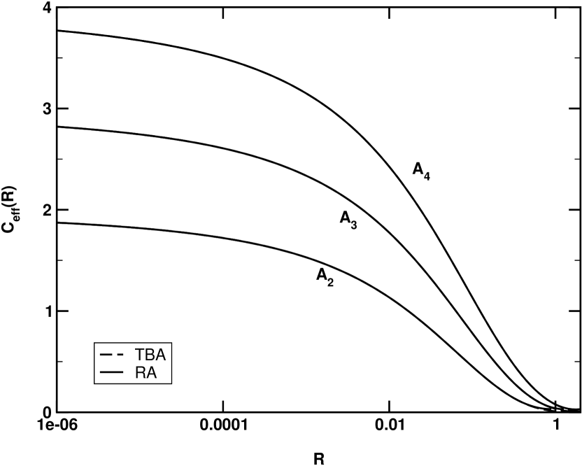
Figure 1: Plot of $c_{\rm eff}$ for $A_{2},A_{3},A_{4}$ ATFTs at $B=0.4$ for $(++)$ BC.

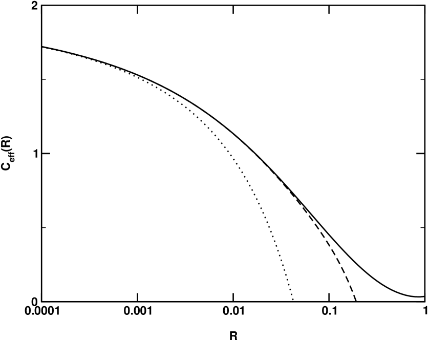
Figure 2: Plot of $c_{\rm eff}$ for $A_{2}$ ATFTs for $(++)$ BC without any vacuum energy (dotted line) and with boundary vacuum energy (dashed line). Including both energies (solid line), two results become identical upto $R\sim{\cal O}(1)$.

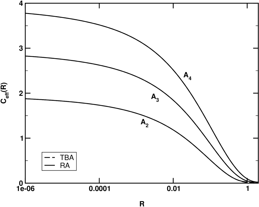
Figure 3: Plot of $c_{\rm eff}$ for $A_{2},A_{3},A_{4}$ ATFTs at $B=0.4$ for $(+f)$ BC.

References

• [1] A. B. Zamolodchikov, Int. J. Mod. Phys. A4 (1989) 4235.
• [2] V. Fateev, S. Lukyanov, A. Zamolodchikov, and Al. Zamolodchikov, Phys. Lett. B406 (1997) 83.
• [3] A. B. Zamolodchikov and Al. B. Zamolodchikov, Nucl. Phys. B477 (1996) 577.
• [4] C. Ahn, C. Kim, and C. Rim, Nucl. Phys. B556 (1999) 505.
• [5] C. Ahn, V. Fateev, C. Kim, C. Rim and B. Yang, Nucl. Phys. B565 (2000) 611.
• [6] Al. B. Zamolodchikov, Nucl. Phys. B342 (1990) 695.
• [7] C. Ahn, P. Baseilhac, V. Fateev, C. Kim, and C. Rim, Phys. Lett. B481 (2000) 114.
• [8] S. Ghoshal and A. B. Zamolodchikov, Int. J. Mod. Phys. A9 (1993) 3841.
• [9] V. Fateev, β€œNormalization Factors, Reflection Amplitudes and Integrable Systems”, hep-th/0103014.
• [10] A. Arinstein, V. Fateev, and A. Zamolodchikov, Phys. Lett. B87 (1979) 389.
• [11] H. W. Braden, E. Corrigan, P. E. Dorey, and R. Sasaki, Nucl. Phys. B338 (1990) 689.
• [12] E. Corrigan, P. Dorey, R. Rietdijk, and R. Sasaki, Phys. Lett. B333 (1994) 83.
• [13] V. A. Fateev, A. Zamolodchikov, and Al. Zamolodchikov, β€œBoundary Liouville Field Theory I. Boundary State and Boundary Two-point Function”, hep-th/0001012.
• [14] Al. B. Zamolodchikov, in private communication.
• [15] A. Fring and R. KΓΆberle, Nucl. Phys. B419 (1994) 647; B421 159.
• [16] R. Sasaki, β€œReflection bootstrap equations for Toda field theory”, hep-th/9311027.
• [17] J.D. Kim, Phys. Lett. B353 (1995) 213.
• [18] E. Corrigan, Int. J. Mod. Phys. A13 (1998) 2709; G. M. Gandenberger, Nucl. Phys. B542 (1999) 659.
• [19] A. LeClair, G. Mussardo, H. Saleur, and S. Skorik, Nucl. Phys. B453 (1995) 581.
• [20] C. Destri and H. de Vega, Nucl. Phys. B358 (1991) 251.
• [21] G. W. Delius and G. M. Gandenberger, Nucl. Phys. B554 (1999) 325.
Refer to caption