CALT-68-2351

CITUSC/01-035

hep-th/0110193

On non-uniform black branes

Steven S. Gubser${}^{\,}$^,

Lauritsen Laboratory of Physics, 452-48 Caltech, Pasadena, CA 91125

Abstract

Certain black branes are unstable toward fluctuations that lead to non-uniform mass distributions. We study static, non-uniform solutions that differ only perturbatively from uniform ones. For uncharged black strings in five dimensions, we find evidence of a first order transition from uniform to non-uniform solutions.

October 2001

1 Introduction

The Gregory-Laflamme instability [1, 2] has been explored principally via linearized perturbation theory and thermodynamic scaling arguments. In its simplest incarnation, it is a tachyonic mode in perturbations around an uncharged black brane which makes the horizon bulge out at some points and squeeze in at others. It is a purely classical effect in Minkowskian signature, and we may think of it crudely as a black brane redistributing its mass in order to gain entropy. Until recently it was commonly supposed that this evolution would proceed until the horizon bifurcated into an array of black holes (and then these black holes might run into one another, clustering mass into ever fewer, ever larger black holes).

This naive view has recently been called into question because of a result of Horowitz and Maeda [3]. These authors demonstrated rigorously that a black hole horizon cannot pinch off in finite affine time, and they give less airtight arguments that such a pinch-off also cannot happen in infinite affine time. Thus it becomes plausible that the endpoint of the evolution is a stable, non-uniform black brane. In the case of a black string, the non-uniform solution might be expected to look like an unbroken string of identical beads.

Briefly, the aim of this paper is to look for such a non-uniform black string using perturbation theory around the uniform solution, and to discuss possible phase transitions between different types of solutions.

The organization of the paper is as follows: in section 2, we discuss order parameters. In section 3, we perform an explicit perturbation analysis around the black string solution in five dimensions. Non-uniform solutions are constructed perturbatively around the uniform string with $\eta=\eta_{c}$. Unfortunately, even this involves some numerical work, which will be explained in some detail in sections 3.2-3.6. In section 4 we make some general remarks about how the Landau theory of phase transitions might bear on non-uniform branes of various dimensionalities, and also comment on possible instabilities which could arise after a brane has become non-uniform. We summarize our key results on the five-dimensional uncharged black string in section 5.

2 Order parameters

The Gregory-Laflamme instability is an infrared effect: when it is present, all accessible wavelengths below a certain threshold are unstable. Life is simpler if one imposes an infrared regulator: for example, one may compactify the directions parallel to the black brane on some torus. Then the instability shows up only if the Schwarzschild radius is sufficiently small compared with the size of the torus (the zero-mode cannot be excited because of energy conservation). The commonly supposed endpoint of the evolution (before [3]) was a single black hole, localized in the torus directions as well as the orthogonal directions. By a simple scaling argument, such a black hole has more entropy for a given mass than the uniform black brane starting point, provided the size of the torus is sufficiently large compared to the Schwarzschild radius of the black brane.

As long as we are discussing solutions of the classical empty space Einstein equations, $R_{\mu\nu}=0$, there is no intrinsic scale in the problem. This may be seen from the fact that a rigid rescaling of the entire metric takes solutions into solutions. The uniform black brane determines a length scale, namely its Schwarzschild radius, $R_{\rm Schwarzschild}$. After compactifying the uniform black brane on a torus, suppose the longest wavelength perturbation accessible has wave number $k_{\rm min}$. Then we may define the figure of merit

$${\eta=R_{\rm Schwarzschild}k_{\rm min}\,.}$$ (1)

For a non-uniform solution, we may still define $\eta$ as the value that would pertain if the non-uniform brane were replaced by a uniform one of the same mass.

If the black brane does become non-uniform, there is another dimensionless number, $\lambda$, which describes how non-uniform it is. Supposing that the rotational symmetry in the directions transverse to the brane is preserved, we can define unambiguously the area of a slice of the horizon over any point along the brane, and hence an effective Schwarzschild radius at any point. Then we can define

$${\lambda={1\over 2}\left({R_{\rm Schwarzschild,\ max}\over R_{\rm Schwarzschild,\ min}}-1\right)\,.}$$ (2)

Thus $\lambda=0$ for the uniform black brane; $\lambda=\infty$ for a black hole localized on the torus, and $\lambda$ is finite for a non-uniform black brane with an unbroken horizon.

A final meaningful number for a non-uniform horizon compactified on a torus (or other manifold for that matter) is the number $n$ of local maxima of the Schwarzschild radius—again on the assumption that transverse rotational symmetry is preserved, so that the Schwarzschild radius has a good local definition everywhere on the brane.

Roughly speaking, the problem gets harder as $\eta$ decreases. For $\eta$ large, the compactification scale is much smaller than another scale in the problem, so we may expect the uniform black brane to be stable and to win out over any other solution. Below some critical $\eta_{c}$, the uniform black brane becomes unstable to small perturbations: this is the Gregory-Laflamme instability. What happens for smaller $\eta$ is not known. Focusing first on the black string, one might reasonably expect that for some range of $\eta$ below $\eta_{c}$, there is a stable solution with finite $\lambda$ and $n=1$. Then the question becomes, does non-zero $\lambda$ develop smoothly or suddenly as one crosses $\eta_{c}$? That is, is the phase transition from uniform to non-uniform black strings continuous or first order? The results of section 3 will suggest that it is first order.

3 Numerics on the black string

3.1 Generalities

At $\eta=\eta_{c}$, the perturbative Gregory-Laflamme instability becomes a zero-mode of the uniform black brane solution, so we may expect that there is a new branch of the solution space heading out to nonzero $\lambda$, but emanating from $\lambda=0$ and $\eta=\eta_{c}$. This new branch has one maximum for the Schwarzschild radius ($n=1$) because the zero mode changes $R_{\rm Schwarzschild}$, multiplicatively, by an amount $1+\lambda\cos kx$ where $k$ is the fundamental wave-number of the black string. A continuous moduli space may seem at odds with first order behavior; see however figure 1(a), equation (33), and the surrounding discussion for a preview of how the two are consistent.

We want static five-dimensional black string solutions to Einstein’s equations in the absence of matter: $R_{\mu\nu}=0$. A general ansatz for such solutions is

$${ds^{2}=-e^{2A}\left(1-{2M\over r}\right)dt^{2}+e^{2B}\left[{dr^{2}\over 1-{2M\over r}}+dz^{2}\right]+e^{2C}r^{2}d\Omega_{2}^{2}\,,}$$ (3)

where $A$, $B$, and $C$ are arbitrary functions of $r$ and $z$. Here we have used diffeomorphism freedom to constrain the ratio of $g_{rr}$ and $g_{zz}$, to get rid of any $g_{rz}$ term, and to ensure that the black string horizon is at $r=2M$. The ansatz (3) is almost in conformal gauge: it would be exactly in conformal gauge if we changed coordinates to $\tilde{r}$ such that $d\tilde{r}^{2}=dr^{2}/(1-2M/r)$. Clearly, if $A=B=C=0$, we have the uniform black string.

It’s possible to change coordinates and rescale the entire metric so that it becomes

$${ds^{2}=-e^{2A}\left(1-{1\over y}\right)dt^{2}+e^{2B}\left[{dy^{2}\over 1-{1\over y}}+dx^{2}\right]+e^{2C}y^{2}d\Omega_{2}^{2}\,.}$$ (4)

The Schwarzschild radius of the uniform solution is $1$. The periodicity of the $x$ direction is $2\pi/\eta$, so $\eta$ coincides with the minimal wave-number $k$ which we can excite. Looking for solutions of the form (4) to $R_{\mu\nu}=0$ amounts to an elliptic boundary value problem: boundary conditions are imposed at the horizon to ensure that it is regular, and other boundary conditions are imposed at infinity to ensure that the solution is asymptotically flat. (Actually, we will see that regularity plus asymptotic flatness are not quite sufficient to fix all integration constants. This subtlety will figure prominently in sections 3.4 and 3.5, but may otherwise be glossed over.) Elliptic boundary value problems for ordinary differential are fairly straightforward to deal with: the basic strategy is some form of “shooting” algorithm, where one artificially imposes full Cauchy data at one end of the integration region, then integrates the ODE’s to the other end, and then checks to see whether the boundary conditions are satisfied there. To understand why elliptic boundary problems are harder for partial differential equations, imagine trying the same strategy, for example imposing Cauchy data at $y=1$ and then integrating out to infinity. One has to discretize the $x$-interval to perform this integration. Intuitively, such a discretization involves about as many Fourier modes as there are pixels. The higher Fourier modes have higher mass. Each of these modes has a solution which grows exponentially at infinity rather than vanishing. Round-off error will tend to source these growing solutions, with the result that numerical integration outward in $y$ quickly diverges, for any initial data at the horizon. It appears in fact that there is no standard algorithm for solving elliptic boundary value problems for non-linear PDE’s. A custom algorithm is usually constructed, based commonly on some global relaxation method, to deal with a specific problem.

Instead of pursuing the intensive numerical route, let us make an expansion around the uniform string:

$${A} {{}=\lambda^{2}a_{0}(y)+\lambda a_{1}(y)\cos kx+\lambda^{2}a_{2}(y)\cos 2kx+O(\lambda^{3})} {B} {{}=\lambda^{2}b_{0}(y)+\lambda b_{1}(y)\cos kx+\lambda^{2}b_{2}(y)\cos 2kx+O(\lambda^{3})} {C} {{}=\lambda^{2}c_{0}(y)+\lambda c_{1}(y)\cos kx+\lambda^{2}c_{2}(y)\cos 2kx+O(\lambda^{3})\,.}$$ (5)

We will work at small $\lambda$, but the coefficient functions are finite. The expansion (5) is appropriate for studying perturbations at the wavelength which is marginally stable. The reason is that at lowest order, $O(\lambda)$, a perturbation at this wavelength is a zero mode of the uniform black brane. At $O(\lambda^{2})$, back-reaction leads to non-trivial $X_{0}$ and $X_{2}$, where $X=a$, $b$, or $c$. If we make a Kaluza-Klein reduction in the $x$ direction, then the $X_{i}$ for $i\neq 0$ are massive modes, while the $X_{0}$ are massless modes. Thus the $X_{i}$ for $i\neq 0$ fall off exponentially for large $y$, while the $X_{0}$ fall off as inverse powers of $y$. So to read off the mass density of the black string, all we need is the $x$-independent modes. We will elaborate on this point later.

Having made the expansion (5), we are left with a finite set of ODE’s at each order in $\lambda$. Boundary conditions still must be imposed both at the horizon and at infinity. Let us now enter into the details of the calculation. The reader uninterested in technical points may wish to skip directly to section 3.7.

3.2 Solution to $O(\lambda)$

The basic ODE’s can be derived by plugging (5) into the Einstein equations, $R_{\mu\nu}=0$. At $O(\lambda)$, one can solve algebraically for $b_{1}(y)$, with the result

$${b_{1}=-{a_{1}+2\,\left(-1+y\right)\,\left(2\,c_{1}+y\,a_{1}^{\prime}+2\,y\,c_{1}^{\prime}\right)\over 3-4\,y}\,,}$$ (6)

where primes denote $d/dy$. This equation incorporates the zero energy constraint. One may also show that the $O(\lambda)$ equations imply

$${b_{1}^{\prime}={2\over-3+4\,y}\left(k^{2}\,y^{2}\,a_{1}+2\,b_{1}-2\,c_{1}+2\,k^{2}\,y^{2}\,c_{1}+2\,a_{1}-2\,y\,a_{1}+c_{1}-2\,y\,c_{1}\right)\,,}$$ (7)

which is a relation which we will find helpful in section 3.4. Eliminating $b_{1}$ from the other differential equations at $O(\lambda)$ leads to

$${2\,k^{2}\,y^{2}\,a_{1}+\left(1-4\,y\right)\,a_{1}^{\prime}-2\,\left(c_{1}^{\prime}+\left(-1+y\right)\,y\,a_{1}^{\prime\prime}\right)} {{}=0} {-2\,a_{1}+\left(2+k^{2}\,\left(3-4\,y\right)\,y^{2}\right)\,c_{1}+3\,a_{1}^{\prime}-3\,y\,a_{1}^{\prime}\qquad} {+9\,c_{1}^{\prime}-16\,y\,c_{1}^{\prime}+8\,y^{2}\,c_{1}^{\prime}-y(-1+y)(3-4\,y)\,c_{1}^{\prime\prime}} {{}=0}$$ (8)

Evidently, the horizon is a regular singular point of these differential equations, which are linear because at $O(\lambda)$ we’re dealing precisely with linearized perturbations around the uniform black string. We can exploit the linearity to get rid of one arbitrary constant: let us say $c_{1}(1)=1$. Examining the region near $y=1$, one can show that two solutions of (8) are singular. Regularity at the horizon demands that these singular solutions should be absent. To specify Cauchy data at the horizon we must therefore specify just one more quantity at the horizon—conveniently $a_{1}(1)$. Also $k$ must be specified. At infinity there are two exponentially growing solutions to (8). The natural boundary conditions at infinity are that these solutions must be absent. Thus we have two free parameters, $a_{1}(1)$ and $k$, and two boundary conditions at infinity to satisfy. An appropriate two-parameter shooting algorithm is easy to implement. The only subtlety worth mentioning is that because we have two growing solutions at infinity, it’s possible to them to compete so that $a_{1}(y)^{2}+c_{1}(y)^{2}$ is small at a single large value of $y$, but large at other values. So to test whether one has eliminated both growing solutions, an efficient and robust method is to integrate $a_{1}(y)^{2}+c_{1}(y)^{2}$ over some interval near the end of the integration region. We have done this, with the result $a_{1}(1)=-0.552$ and $k=0.876$. This value of $k$ is in accord with the results of [1].

3.3 Mass, entropy, and temperature

Before going on to $O(\lambda^{2})$, let us describe in more detail how the mass and entropy can be calculated. The results in this section are valid at any order in $\lambda$, and indeed make almost no reference to the expansion (5). Following [6], we define the mass as

$${E=-{1\over 8\pi}\int_{\Sigma}\left({}^{3}K-{}^{3}K_{0}\right)\,,}$$ (9)

where ${}^{3}K$ is the trace of the extrinsic curvature of a surface $\Sigma$ at constant $y$ and $t$, computed with respect to the four-dimensional spatial metric: that is,

$${{}^{3}K={1\over\sqrt{{}^{4}g}}\partial_{i}\left(\sqrt{{}^{4}g}N^{i}\right)\,,}$$ (10)

where ${}^{4}g$ is the metric on a $t=const$ spatial slice, and $N^{i}$ is the unit normal to the surface $y=const$ in this slice. The quantity ${}^{3}K_{0}$ is the extrinsic curvature for a reference geometry, in our case flat space. A large $y$ limit is taken after subtracting the contribution of the reference geometry, and then the energy should be finite. In making the subtraction, the surface $\Sigma$ must be chosen to have the same induced geometry in the black string background and the reference geometry, at least up to a sufficiently high order in large $y$. In our case, we may altogether ignore the functions $X_{i}$ for $i\neq 0$ (effectively setting them equal to $0$) because at large $y$ they fall off exponentially in $y$, whereas the terms in ${}^{3}K-{}^{3}K_{0}$ that make finite contributions to the energy are $O(1/y^{2})$. Let us assume the leading order behavior

$${B={B_{\infty}\over y}+O(1/y^{2})\qquad C={C_{\infty}\log y\over y}+O(1/y)\,.}$$ (11)

Then, suppressing all exponentially small corrections, we can write

$${\sqrt{{}^{4}g}} {{}=e^{2B+2C}{y^{2}\over\sqrt{1-1/y}}\qquad N^{y}=e^{-B}\sqrt{1-1/y}} {{}^{3}K} {{}={1\over\sqrt{{}^{4}g}}\partial_{y}\left(\sqrt{{}^{4}g}N^{y}\right)={\sqrt{1-1/y}\over y^{2}}e^{-2B-2C}\partial_{y}\left(e^{B+2C}y^{2}\right)} {{}={2\over y}-2C_{\infty}{\log y\over y^{2}}-{1\over y^{2}}(1+3B_{\infty}-2C_{\infty})+O(1/y^{3})\,,}$$ (12)

This is to be compared with ${}^{3}K_{0}=2/y_{0}$ for the flat reference spacetime. However, in making the subtraction one does not want $y_{0}=y$, but rather $y_{0}=ye^{C}=y+C_{\infty}\log y+O(1/y)$ so that the $S^{2}$ has the same curvature in the black string geometry and the reference geometry. Thus we obtain

$${{}^{3}K_{0}} {{}={2\over y}-2C_{\infty}{\log y\over y^{2}}} {{}^{3}K-{}^{3}K_{0}} {{}={1\over y^{2}}(1+3B_{\infty}-2C_{\infty})+O(1/y^{3})\,.}$$ (13)

The area of the $S^{2}$ is $4\pi y^{2}$, and the length of the $S^{1}$ is $2\pi/k$, so we see that the energy of the black string is $(1+3B_{\infty}-2C_{\infty})/k$ up to overall constants. In later sections we will allow $k$ to vary, so it is more convenient to define $e=kE/2\pi$ as the average energy density. Then

$${{\delta e\over e}=3B_{\infty}-2C_{\infty}\,.}$$ (14)

In applying the result (14), it must be recalled that we assumed (11). In a perturbative treatment in $\lambda$, one must check this asymptotic behavior at any given order. Most modifications of the asymptotics would render the mass infinite.

Computing the entropy is more straightforward: it is just the horizon area over $4G_{5}$, so the fractional change in the average entropy density, $s=kS/2\pi$, is

$${{\delta s\over s}=\left\langle e^{B+2C}\Big{|}_{y=1}\right\rangle-1\,,}$$ (15)

where $\langle\rangle$ means to average over the $x$ direction. Thus $(\delta s)/s$ winds up being some combination of the $X_{i}$ evaluated at $y=1$.

The temperature is also easy to compute, using for instance the standard prescription of rotating to Euclidean signature and demanding no conical deficit at the horizon. The result is

$${{\delta T\over T}=e^{A-B}\Big{|}_{y=1}-1}$$ (16)

The right hand side is not manifestly independent of $x$. A convenient check on boundary conditions at the horizon is to verify that they preclude any contribution to $(A-B)\big{|}_{y=1}$ other than from zero modes.

3.4 The zero modes at $O(\lambda^{2})$

As per the discussion of the previous section, to compute $(\delta e)/e$ and $(\delta s)/s$ to $O(\lambda^{2})$, all we require is the functions $X_{0}$ to this order (where as usual, $X$ can be $a$, $b$, or $c$). So we postpone discussion of the $X_{2}$ until section 3.5.

The equations for the zero modes at $O(\lambda^{2})$ are rather complicated. All the relevant equations take the schematic form $X_{0}=X_{1}^{2}$, where the left hand side denotes some linear combination of $a_{0}$, $b_{0}$, $c_{0}$ and their first and second derivatives, and the right hand denotes a quadratic expression in $a_{1}$, $b_{1}$, $c_{1}$ and their first and second derivatives. Using (6), (7), and (8), one can eliminate all second derivatives from the right hand side of $X_{0}=X_{1}^{2}$, and also eliminate all dependence on $b_{1}$ and $b_{1}^{\prime}$. (This is a good idea for numerics, because the functions $X_{1}$ are known only numerically, and differentiating them leads to more numerical noise.) One of the resulting equations is

$${-{d\over dy}2(-1+y)y{d\over dy}b_{0}} {{}={2\,y\over{\left(3-4\,y\right)}^{2}}\Big{(}2\,k^{2}\,y\,\left(3-7\,y+4\,y^{2}\right)\,{a_{1}}^{2}+k^{2}\,y\,\left(-3+4\,y\right)\,{c_{1}}^{2}} {{}\quad{}-2\,\left(-1+y\right)\,c_{1}\,\left(a_{1}^{\prime}+2\,c_{1}^{\prime}\right)} {{}\quad{}-\left(3-5\,y+2\,y^{2}\right)\,\left(2\,\left(-1+y\right)\,a_{1}^{\prime}-c_{1}^{\prime}\right)\,\left(a_{1}^{\prime}+2\,c_{1}^{\prime}\right)} {{}\quad{}+a_{1}\,\Big{(}k^{2}\,y\,\left(-3+10\,y-8\,y^{2}\right)\,c_{1}+2\,\left(-1+y\right)\,\left(a_{1}^{\prime}+2\,c_{1}^{\prime}\right)\Big{)}\Big{)}.}$$ (17)

This equation is easy to integrate twice numerically. In order to have regularity at the horizon, $b_{0}(1)$ must be finite, and this fixes a constant in the first integration. The constant in the second integration can be fixed by demanding $b_{0}\to 0$ as $y\to\infty$. This boundary condition does not come from asymptotic flatness, but it could be arranged through some rescalings. No shooting is necessary. After integrating, one can easily extract $B_{\infty}\approx 0.41\lambda^{2}$.

The other equations derivable at $O(\lambda^{2})$ for the zero modes take the form

$${a_{0}^{\prime}-4\,y\,a_{0}^{\prime}-2\,c_{0}^{\prime}+2\,y\,a_{0}^{\prime\prime}-2\,y^{2}\,a_{0}^{\prime\prime}} {{}=S_{1}(a_{1},c_{1})} {-4\,c_{0}+2\,a_{0}^{\prime}-2\,y\,a_{0}^{\prime}+6\,c_{0}^{\prime}-8\,y\,c_{0}^{\prime}+2\,y\,c_{0}^{\prime\prime}-2\,y^{2}\,c_{0}^{\prime\prime}} {{}=S_{2}(a_{1},c_{1};b_{0})} {8\,c_{0}-8\,a_{0}^{\prime}+8\,y\,a_{0}^{\prime}-4\,c_{0}^{\prime}+8\,y\,c_{0}^{\prime}} {{}=S_{3}(a_{1},c_{1};b_{0})\,,}$$ (18)

where the source terms $S_{1}$, $S_{2}$, and $S_{3}$ are quadratic expressions in $a_{1}$, $c_{1}$ and their first derivatives, like the right hand side of (17). $S_{2}$ and $S_{3}$ also have linear dependence on $b_{0}$. We regard $b_{0}$ as fixed from the considerations of the previous paragraph. Note that $a_{0}$ appears only through its derivatives. An additive shift of $a_{0}$ corresponds to a multiplicative redefinition of $t$. The equations in (18) are not independent: the first, for example, follows from the second and the third together. For numerics, it would seem most straightforward to keep the third equation and drop either the first or the second, since the third is first order. However, it turns out to be better to drop the third equation and integrate the first two numerically. In order to do this we need Cauchy data at the horizon. If we assume regularity of $a_{0}$, $c_{0}$ and their first and second derivatives, then by setting $y=1$ in the first and third equations in (18) we obtain

$${-3a_{0}^{\prime}-2c_{0}^{\prime}=S_{1}(a_{1},c_{1})\,,\qquad-4c_{0}(1)-2c_{0}^{\prime}(1)=S_{2}(a_{1},c_{1};b_{0})\,,}$$ (19)

where all quantities are evaluated at $y=1$. The third equation in (18) does not lead to any additional boundary conditions at the horizon. Two more boundary conditions are required to complete the Cauchy data: one of them is the trivial additive constant on $a_{0}$, which can be adjusted a posteriori so that $a_{0}(y)\to 0$ as $y\to\infty$; and the other is the value of $c_{0}(1)$. Any choice of $c_{0}(1)$ leads to a solution that is regular everywhere, with asymptotics as in (11). The $O(\lambda^{2})$ contribution to $C_{\infty}$ depends on $c_{0}(1)$.

Clearly this leaves us with a puzzle: why is $C_{\infty}$, and hence the mass, indeterminate? Roughly, the answer is that, at the order to which we are working, we are still free to “superpose” an arbitrary $O(\lambda^{2})$ change in the mass of the black hole on top of the change that the non-uniformity induces. The value of $c_{0}(1)$ is undetermined at $O(\lambda^{2})$, and will be fixed, if at all, by considerations at higher order. (We will revisit this issue in section 3.5.) The equations (18) with the $S_{i}$ set to $0$ correspond precisely to perturbations of a Schwarzschild black hole in four dimensions in a gauge where the radial part of the metric is exactly $dy^{2}/(1-1/y)$. With this choice of gauge, an increase of the mass of the black hole is expressed as a solution to the homogeneous equations derived from (18) with $c_{0}(y)\sim C_{\infty}(\log y)/y$ for large $y$. Any multiple of this solution to the homogeneous equations can be added to a solution to the inhomogeneous equations: that is the origin of the ambiguity in the mass.

To proceed, let us set $c_{0}(1)=0$. Numerical integration of (18) is now straightforward. Summarizing the results of the numerics so far:

$${a_{1}(1)=-0.55\qquad b_{1}(1)=-0.55\qquad c_{1}(1)=1} {a_{0}(1)=0.53\qquad b_{0}(1)=0.77\qquad c_{0}(1)=0} {B_{\infty}=0.41\lambda^{2}\qquad C_{\infty}=0.29\lambda^{2}\,.}$$ (20)

Given these values, together with (14) and (15), one may evaluate, to $O(\lambda^{2})$,

$${{\delta e\over e}} {{}=3B_{\infty}-2C_{\infty}\approx 0.64\lambda^{2}} {{\delta s\over s}} {{}=\left[b_{0}+2c_{0}+{1\over 4}b_{1}^{2}+b_{1}c_{1}+c_{1}^{2}\right]_{y=1}\lambda^{2}\approx 1.29\lambda^{2}\,.}$$ (21)

Adjusting $c_{0}(1)$ changes $(\delta s)/s$ by exactly twice the amount that it does $(\delta e)/e$: this is because the entropy-mass relation for the four-dimensional Schwarzschild solution is $S\propto M^{2}$. A quantity which is supposed to be independent of $c_{0}(1)$ is

$${\Delta_{es}={\delta s\over s}-2{\delta e\over e}=\sigma_{1}\lambda^{2}\qquad\hbox{where}\quad\sigma_{1}\approx 0.002\,.}$$ (22)

The coefficient $\sigma_{1}$ is remarkably small compared to the values in (20). This may lead us to suspect that the true value is zero, so that the non-zero result in (22) is pure round-off error. We will presently give an entirely analytical demonstration that $\sigma_{1}=0$; however, let us for the moment examine how we would judge just from the numerics whether $(\ref{DeltaES})$ is consistent with a zero result. One way way to test this hypothesis is to vary $c_{0}(1)$ and see how much $\sigma_{1}$ changes. Since all the values in (20) are on the order of unity, it would seem natural for $c_{0}(1)$ to have a similar magnitude. So the deviations in the result that come from assigning $c_{0}(1)$ the values $\pm 1$ rather than $0$ are something like a standard deviation. This “standard deviation” turns out to be roughly $0.02$, so our result is indeed consistent with $\sigma_{1}=0$ (in fact, one might say that we were lucky to get a value as small as the one in (22)). Another test is to upgrade the numerics in various ways and see what changes. The results quoted in (20)-(22) come from the last of five iterations of improvement, which added about one decimal place of accuracy. The first three iterations were about one standard deviation positive.

The bottom line is that numerics are consistent with the hypothesis that, at $O(\lambda^{2})$, a uniform black string and a non-uniform one with the same mass also have the same entropy. More precisely, the non-uniform black string’s entropy exceeds that of the uniform black string only by about one standard deviation, as defined heuristically in the previous paragraph. Now let us show analytically that $\Delta_{es}=o(\lambda^{2})$, using the First Law of thermodynamics (which certainly should hold for the non-uniform solutions at hand, since as static solutions to the vacuum Einstein’s equation they have well-defined event horizons). We will need to assume that, if the asymptotic size of the $S^{1}$ is held fixed, then the mass is specified unambiguously once one has specified $\lambda$. That this is true will emerge from the discussion in section 3.5. Thus there is a one-parameter curve of non-uniform solutions in the $\eta$-$\lambda$ plane, emanating from the point $(\eta_{c},0)\approx(0.876,0)$. Suppose we slide incrementally along this curve, away from $(\eta_{c},0)$. Then the First Law says $dE=T_{c}dS$, where $T_{c}$ is the temperature at $(\eta_{c},0)$. At this point, the black hole is uniform, so we may use the standard four-dimensional Schwarzschild relation $T_{c}=E_{c}/(2S_{c})$. Rearranging the first law slightly, we obtain $2(dE)/E_{c}=(dS)/S_{c}$. Thus indeed $\Delta_{es}=0$, at least to some lowest order. Now we have to explain why this works to $O(\lambda^{2})$. The reason is that the temperature deviates from $T_{c}$ only at $O(\lambda^{2})$, and then this small deviation is further suppressed (to $O(\lambda^{4})$, in fact) when one integrates the infinitesimal form of the First Law out from $0$ to $\lambda$.

The assumption that the asymptotic size of the $S^{1}$ is constant is needed in the above derivation because otherwise the First Law would have an additional term corresponding to variations in this quantity. The assumption that only a one-parameter family of non-uniform solutions exists with fixed asymptotic size of $S^{1}$ is needed for the same reason: otherwise there would effectively be another thermodynamic observable that would contribute to the First Law.

Obviously, although we may feel relieved that our numerics through $O(\lambda^{2})$ passes one non-trivial analytical check, we should also feel disappointed that no really meaningful numbers came out of the analysis so far, beyond what is in the literature. To do better we must proceed at least to $O(\lambda^{3})$. There are some conceptual subtleties involved, which we will discuss in the next section.

3.5 Higher orders in perturbation theory

To organize higher order in perturbation theory, it will be useful to consider the expansions

$${A} {{}=\sum_{n=0}^{\infty}\lambda^{n}A_{n}\cos nKx} {B} {{}=\sum_{n=0}^{\infty}\lambda^{n}B_{n}\cos nKx} {C} {{}=\sum_{n=0}^{\infty}\lambda^{n}C_{n}\cos nKx\,,}$$ (23)

where for $X=A$, $B$, and $C$ we have the additional expansions

$${X_{n}=\sum_{p=0}^{\infty}\lambda^{2p}X_{n,p}\,,}$$ (24)

and now the $X_{n,p}$ are independent of $\lambda$. Also $K$ itself may be taken to have an expansion in $\lambda$,

$${K=\sum_{q=0}^{\infty}\lambda^{2q}k_{q}\,.}$$ (25)

Translating back into the notation of (5), we have $k_{0}=k$, $A_{0,0}=0$, $A_{0,1}=a_{0}$, $A_{1,0}=a_{1}$, $A_{2,0}=a_{2}$, and the same for $B$ and $C$. We do not see any reason for non-analytic terms in $\lambda$ to appear at any order in (23) or (24), or for odd powers of $\lambda$ to appear in (24) or (25). If either thing happened, then it would seem likely that there are additional physical constants of integration to specify beyond $\eta$ and the ratio of minimum and maximum radius for the horizon.

Given the results of previous sections, it should be plausible that the Einstein equations $R_{\mu\nu}=0$ boil down to an infinite set of ODE’s of the form

$${{\cal L}^{X}_{n}[X_{n,p}]=S_{X_{n,p}}\,.}$$ (26)

The left hand side represents a first or second linear differential operator ${\cal L}^{X}_{n}$ operating on the $X_{n,p}$. Linear equations for $X_{n,p}$ arise at $O(\lambda^{n+2p})$. For $n\neq 0$, the form of these differential operators is identical to the forms in equations (6), (7), (8), only with $k$ replaced by $nk_{0}$. The right hand side of (26) represents a sum of terms, each expressible as a product of several $X_{n_{i},p_{i}}$ and their derivatives, as well as various $k_{q_{j}}$, subject to two sum rules: $\sum_{i}s_{i}n_{i}=n$, where each $s_{i}=\pm 1$, and $\sum_{i}(n_{i}+2p_{i})+\sum_{j}q_{j}=n+2p$. The first of these rules comes from Fourier analysis, and the second comes from power counting in $\lambda$. This means that one may solve the equations (26) order by order in $\lambda$ (that is, in order of increasing $n+2p$)—modulo a difficulty to be discussed below. At a given order in $\lambda$, the equations with different $n$ are independent. There is a further useful property of the equations (26), easily demonstrated order-by-order: for $n\neq 0$, one can find algebraic expressions for $B_{n,p}$ and $B_{n,p}^{\prime}$ in terms of $A_{n,p}$, $C_{n,p}$, and other $X_{n,p}$ of lower order, and first derivatives of these quantities. For $n=0$, this is not possible.

A subtler point is how we determine all the constants of integration, including the $k_{q}$. There is some freedom on how this is done, corresponding to two obvious considerations: first, we have not entirely fixed the diffeomorphism freedom with the ansatz (4) and (23); second, starting at second order in $O(\lambda^{2})$, one has the freedom to simultaneously add something to the mass and change $K$, in essence rescaling the solution by a perturbatively small amount. Even after demanding that $A(x,y)$, $B(x,y)$, and $C(x,y)$ vanish in the limit $y\to\infty$, there is some ambiguity left. To “fix a scheme,” one could for example say $X_{0,0}=0$, $C_{0,p}(1)=0$ for all $p$, $C_{1,0}(1)=1$, and $C_{1,p}(1)=0$ for $p>0$. Then the $k_{q}$ would be fixed as an integration constant in the equations for $X_{1,q+1}$. We will call this the standard scheme.

To make the discussion more definite, let us consider the standard scheme through the first few orders in perturbation theory. At $O(\lambda)$, we have only the $X_{1,0}$ equations, and these fix two integration constants, which in the standard scheme are $k_{0}$ and $A_{1,0}(1)$. At $O(\lambda^{2})$, the requirement that $A(x,y)$ and $C(x,y)$ should vanish as $y\to\infty$ fixes $A_{0,1}(1)$ and $B_{0,1}(1)$, while $C_{0,1}(1)$ is set to zero as part of the standard scheme. This is an arbitrary resolution of the ambiguity we encountered in section 3.4. Also we have at $O(\lambda^{2})$ the equations for $X_{2,0}$, and asymptotic flatness fixes the integration constants $A_{2,0}(1)$ and $C_{2,0}(1)$. Finally, at $O(\lambda^{3})$, we have the equations for $X_{1,1}$ and $X_{3,0}$. The latter are similar to the $X_{2,0}$ equations, and asymptotic flatness fixes $A_{3,0}(1)$ and $C_{3,0}(1)$; the former are similar to the $X_{1,0}$ equations, and in our scheme of setting $C_{1,1}(1)=0$ they fix $k_{1}$ and $A_{1,1}(1)$. As an illustration of how schemes might be altered, we could leave $C_{0,1}(1)$ free in the analysis of the $X_{0,1}$ equations, but set $k_{1}=0$ as well as $C_{1,1}(1)=0$ in the analysis of the $X_{1,1}$ equations, which would leave us with $C_{0,1}(1)$ and $A_{1,1}(1)$ as the constants of integration which are fixed by asymptotic flatness in the analysis of the $X_{1,1}$ equations. This scheme is computationally disadvantageous because when one changes $C_{0,1}(1)$, it is necessary to re-integrate the $X_{0,1}$ equations before solving the $X_{1,1}$ equations. Physically, the new scheme corresponds to holding fixed the asymptotic size of the $S^{1}$ around which the black string is wrapped, whereas the standard scheme allows this asymptotic size to vary at $O(\lambda^{2})$ but sets to zero a particular $O(\lambda^{2})$ contribution to the change in mass. Naively, one might propose yet another scheme where the total mass is held fixed at $O(\lambda^{2})$ and $k_{1}=0$ as well, but $C_{1,1}(1)$ is left free, in which case $A_{1,1}(1)$ and $C_{1,1}(1)$ would be the constants of integration fixed by analysis of the $X_{1,1}$ equations. This seems natural, but in fact we suspect that this scheme is degenerate, because it takes us out toward non-zero $\lambda$ on a curve where $\eta$ is constant at least to $O(\lambda^{2})$. The dependence of $\eta$ on $\lambda$ at lowest non-trivial order is part of the physical “output” of our numerics, and so should not be fixed as part of an arbitrary scheme.

Let us now to summarize our immediate aims without getting too tangled up in schemes: we want to pin down the $O(\lambda^{2})$ change in the mass of the string which was left undetermined in section 3.4. To do it we have to proceed to $O(\lambda^{3})$. A clever trick is to fix $(\delta e)/e$ arbitrarily at $O(\lambda^{2})$, but instead allow the size of the $S^{1}$ to change at $O(\lambda^{2})$. That’s equivalent because we can always rigidly rescale the whole solution to bring the size of the $S^{1}$ back to what it was, and in the process recover unambiguously the desired $O(\lambda^{2})$ contribution to $\delta e$.

So far, we have not discussed the $X_{2,0}$ equations in any detail; indeed, the analysis of them is a rather uninteresting replay of the $X_{1,0}$ equations. Let us only remark that $B_{2,0}$ can be determined algebraically, and the remaining two equations are second order in $A_{2,0}$ and $C_{2,0}$, and involve source terms which can be written as quadratic expressions in $A_{1,0}$, $C_{1,0}$, and their first derivatives. Regularity at the horizon fixes $A_{2,0}^{\prime}(1)$ and $C_{2,0}^{\prime}(1)$ once $A_{2,0}(1)$ and $C_{2,0}(1)$ are known. These latter two quantities must be fixed arbitrarily to carry out a numerical integration, and their values then are determined by the requirement that both $A_{2,0}$ and $C_{2,0}$ shrink exponentially for large $y$ rather than growing. The result is

$${A_{2,0}(1)=0.34\,,\qquad C_{2,0}(1)=-0.69\,.}$$ (27)

The $X_{2,0}$ equations are completely independent of the $X_{0,1}$ equations, so the arbitrariness of $C_{0,1}(1)$ does not affect (27).

At $O(\lambda^{3})$, the $X_{1,1}$ equations and the $X_{3,0}$ equations are independent. We have not analyzed the $X_{3,0}$ equations in any detail, but clearly they will turn out just like the $X_{2,0}$ equations: $B_{3,0}$ will be determined algebraically, and $A_{3,0}(1)$ and $C_{3,0}(1)$ will be fixed by normalizability at infinity. It is the $X_{1,1}$ equations that will primarily interest us for the rest of this section. Once again, $B_{1,1}$ can be algebraically eliminated, and what is left is linear second order equations for $A_{1,1}$ and $C_{1,1}$, sourced by expressions up to cubic in the $X_{1,0}$, and also depending on $k_{1}$, $X_{0,1}$, and $X_{2,0}$. The form of the homogeneous equations (that is, with the source terms set artificially to zero) is identical to (18), only with $a_{1}$ replaced by $A_{1,1}$ and $c_{1}$ by $C_{1,1}$ (this is a general fact, indicated in (26) by the dependence of ${\cal L}^{X}_{n}$ only on $X$ and $n$, not $p$). In our standard scheme, $k_{1}$ and $A_{1,1}(1)$ are determined by normalizability of $A_{1,1}$ and $C_{1,1}$ at infinity, so there is a two-parameter shooting problem. The results of numerics are

$${k_{1}=0.70\,,\qquad A_{1,1}(1)=-0.24\,.}$$ (28)

The best way to extract the effect on the mass is to return to our definition of $\eta$. For the five-dimensional black string, the “average” Schwarzschild radius appearing in (1) is proportional to the average energy density $e$, so $\eta$ can be expressed as $eK$ up to a factor which includes a power of Newton’s constant. Combining the $O(\lambda^{2})$ effects from (21) and (28) (both of which were computed in the standard scheme), we find

$${{\delta\eta\over\eta}={\delta e\over e}+{\delta K\over K}=\eta_{1}\lambda^{2}\qquad\hbox{where}\quad\eta_{1}\approx 1.45\,.}$$ (29)

Because $\eta$ is independent of rigid rescalings of the entire solution, $\eta_{1}$ should be scheme-independent. In fact, there is approximately $0.6\%$ variation in $\eta_{1}$ when $C_{0,1}(1)$ is changed from $0$ to $1$, and much smaller variation when $C_{1,1}(1)$ is changed from $0$ to $1$.

It is possible to extend the First Law argument of section 3.4 to a computation of the entropy difference of the uniform and non-uniform solutions to $O(\lambda^{4})$. Again holding the asymptotic size of the $S^{1}$ fixed, let us integrate the infinitesimal form of the First Law along the curve of non-uniform black brane solutions, starting from the point where it joins onto the uniform solutions, and assuming expansions

$${M=\sum_{p=0}^{\infty}M_{p}\lambda^{2p}\qquad S=\sum_{p=0}^{\infty}S_{p}\lambda^{2p}\qquad T=\sum_{p=0}^{\infty}T_{p}\lambda^{2p}\,.}$$ (30)

Starting with $M_{0}=2T_{0}S_{0}$ (true because at $\lambda=0$ the equation of state is the same as for the four-dimensional Schwarzschild black hole) one quickly obtains $M_{1}/M_{0}=S_{1}/(2S_{0})$ and $M_{2}/M_{0}=S_{2}/(2S_{0})+T_{1}S_{1}/(4T_{0}S_{0})$. Now let us inquire how the entropy of a uniform string changes if we change the mass by $\Delta M$. Since $S\propto M^{2}$, we have $(\Delta S)/S_{0}=2(\Delta M)/M_{0}+[(\Delta M)/M_{0}]^{2}$. What we really want is the difference between the entropy of a non-uniform string and a uniform one of the same mass. So we set $\Delta M=M_{1}\lambda^{2}+M_{2}\lambda^{4}$ and obtain, to $O(\lambda^{4})$,

$${{}{S_{\rm non-uniform}-S_{\rm uniform}\over S_{\rm uniform}}={S_{\rm non-uniform}-S_{\rm uniform}\over S_{0}}} {{}\qquad\qquad{}={S_{1}\over S_{0}}\lambda^{2}+{S_{2}\over S_{0}}\lambda^{4}-{2\Delta M\over M_{0}}-\left({\Delta M\over M_{0}}\right)^{2}=-\left[{T_{1}M_{1}\over T_{0}M_{0}}+\left({M_{1}\over M_{0}}\right)^{2}\right]\lambda^{4}} {{}\qquad\qquad{}=-\left({\delta T\over T}-{\delta K\over K}\right){\delta\eta\over\eta}-\left({\delta\eta\over\eta}\right)^{2}\,.}$$ (31)

The first equality holds, even though $S_{\rm uniform}$ deviates from $S_{0}$ by $O(\lambda^{2})$, because the numerator is an $O(\lambda^{4})$ quantity. In the final equality, we have used the fact that $\eta$ is proportional to $M$, and the constant of proportionality is fixed if the asymptotic size of $S^{1}$ is held fixed. We have also used the facts that $\lambda^{2}T_{1}/T_{0}=(\delta T)/T$ when the asymptotic size of $S^{1}$ is held fixed, and that $(\delta T)/T-(\delta K)/K$ is a scheme-independent quantity at $O(\lambda^{2})$. The final two expressions in (31) involve only quantities computed at $O(\lambda^{2})$, so with (28) in hand one can compute, to the relevant orders,

$${{\delta T\over T}-{\delta K\over K}\approx-1.04\lambda^{2}} {{S_{\rm non-uniform}-S_{\rm uniform}\over S_{\rm uniform}}=\sigma_{2}\lambda^{4}\qquad\hbox{where}\quad\sigma_{2}\approx-0.59\,.}$$ (32)

The coefficients quoted were computed in the standard scheme. There is approximately $3\%$ variation in $\sigma_{2}$ when $C_{0,1}(1)$ is changed from $0$ to $1$, and much smaller variation when $C_{1,1}(1)$ is changed from $0$ to $1$. The value of $\sigma_{2}$ could be used as a consistency check on numerics at $O(\lambda^{4})$, just as the near-vanishing of $\sigma_{1}$ was used in section 3.4 as a consistency check at $O(\lambda^{2})$.

The $0.6\%$ variation in $\eta_{1}$ upon changing $C_{0,1}(1)$ from $0$ to $1$, and the $3\%$ variation in $\sigma_{2}$, are indications of the size of numerical errors, since in principle the quantities in (32) are scheme-independent. Additively, the variation in $\sigma_{2}$ is only twice as large as the variation in $\eta_{1}$, and it is nearly the same as the variation in $\sigma_{1}$ discussed in the paragraph following equation (22). The upshot is that the variations observed in these three quantities are consistent with one another, and small enough that we can be quite confident that $\eta_{1}>0$ and $\sigma_{2}<0$.

3.6 Improving and extending the numerics

There are various ways in which the numerics discussed in previous sections could be improved and extended. To begin with a rather technical point, we have run all our numerics with Mathematica’s built-in NDSolve routine, which uses adaptive step-sizing: the discrete steps can change each time one solves a differential equation with different initial conditions. This results in decreased stability for shooting algorithms which became particularly noticeable in the analysis of the $X_{2,0}$ equations. Fixing the step size once and for all would have its advantages where stability is concerned, although one would probably want to retain the feature that shows up with NDSolve, that the steps are smaller near the horizon. Another technical point which could clearly stand some improvement is the treatment of initial conditions. The rough-and-ready method we have used is to observe that second derivative terms cancel out of the differential right at the horizon, so evaluating the equations there results in a constraint on first derivatives—but one which we then impose at a slight distance away from the horizon (on the order of $10^{-4}$) so that NDSolve won’t be faced with excessively small coefficients on the second derivative terms. A better method, though more labor-intensive, would be to obtain analytic approximations to the regular solutions to some moderate order, and use them as the seed for numerics. (This is straightforward in principle because the horizon is a regular singular point of the differential equations). It might even be hoped that if one knew the near-horizon asymptotics as well as the long-distance tails to sufficiently high order, a reasonably uniform approximation to the $X_{n,p}$ could be obtained via matching. This is not an approximation that could be controlled by a small parameter, as it is in black hole absorption at low energy. It might nevertheless be useful for large $n$, where numerics gets harder and harder due to the increasingly powerful exponentials in the growing solutions.

To determine $C_{\infty}$ at any even order in $\lambda$, we have to distinguish a $(\log y)/y$ behavior from a $1/y$ behavior in a function, $c_{0}(y)$, known only numerically. This is one of the hardest aspects of the numerics, so it is natural to suspect that it is a dominant source of numerical error. The quantities $\sigma_{1}$, $\eta_{1}$, and $\sigma_{2}$ all depend on evaluations of $C_{\infty}$, and all three displayed variations of similar magnitude (of order $10^{-2}$) when the scheme was changed. On the other hand, spot checks of the values of the components of the Ricci tensor gave values on the order of $10^{-15}$ up to $O(\lambda^{3})$, when numerical evaluation was performed after elimination of all second derivatives. This is only ten times the working precision for most executions of NDSolve. These numerical observations are consistent with the hypothesis that the determination of $C_{\infty}$ dominates the numerical error.

In the end, customized code would be needed to optimize results. We have aimed in this paper to avoid excessively hard-core numerics, extracting instead what information we could from standard tools. The total amount of CPU time needed to check all the numbers presented in this paper is roughly an hour on a 800 MHz Pentium PC.

3.7 Interpreting the numerics

Broadly speaking, the goal of this paper has been to make some dent in the problem of constructing stationary non-uniform black brane solutions and elucidating their thermodynamic properties. Our point of entry was the observation that there is a zero-mode fluctuation for the uncharged black string in five dimensions, with wave-number $k=0.876/R_{\rm Schwarzschild}$. This suggests that there is a one-parameter family of non-uniform solutions in the $\eta$-$\lambda$ plane that joins onto the uniform solutions at a “critical point,” $(\eta_{c},\lambda_{c})=(0.876,0)$. We may then ask,

1. What curve in the $\eta$-$\lambda$ plane is traced out by these non-uniform solutions?

2. What is the entropy along this curve?

3. How does a black string behave in real time as one slowly adds mass or allows mass to slowly Hawking radiate away, such that $\eta$ passes through $\eta_{c}$?

A perturbative expansion in small $\lambda$ seems well-suited to study the first two questions near the critical point. Given the answers to these two questions, we can apply the Second Law plus some “natural” assumptions to give a qualitative answer to the third.

Possible answers we could envisage to questions 1 and 2 are sketched in figure 1. Given the analyticity properties in $\lambda$ of the perturbation expansion, we expect

$${\eta=\eta_{c}+\sum_{p=1}^{\infty}\lambda^{2p}\eta_{p}} {\sigma\equiv{S_{\rm non-uniform}\over S_{\rm uniform}}=1+\sum_{p=1}^{\infty}\lambda^{2p}\sigma_{p}\,,}$$ (33)

for some coefficients $\eta_{p}$ and $\sigma_{p}$. In the first line of (33), as in (31) and (32), $S_{\rm non-uniform}$ and $S_{\rm uniform}$ are the entropies of black string solutions with the same mass.

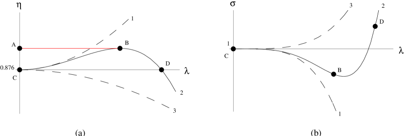
Figure 1: (a) Possible curves, drawn schematically in the $\eta$-$\lambda$ plane, describing stationary, uncharged, non-uniform black strings in five dimensions. The solid curve is the likeliest. (b) $\sigma$ versus $\lambda$ for these non-uniform strings. Again, the solid curve is the likeliest.

The First Law guarantees that $\sigma_{1}=0$, and this was verified to good accuracy by the numerics through $O(\lambda^{2})$ (see (22) and the discussion below it). Numerics through $O(\lambda^{3})$ led to a positive result for $\eta_{1}$ (see (29)). Combining these numerics with First Law considerations further predicts $\sigma_{2}<0$ (see (32)). Thus by our calculations of the previous few sections, we rule out the curves marked (3) in figure 1.

Although we have no direct evidence, it would seem sensible that $\eta<\eta_{c}$ and $\sigma>1$ for sufficiently large $\lambda$. The first inequality guarantees that, for some range of $\eta$ less than $\eta_{c}$, there are stationary solutions with finite $\lambda$ and a single maximum ($n=1$). The second inequality says that these solutions are accessible as the endpoint of Gregory-Laflamme evolution for an unstable uniform string of nearly the same mass. Taking these inequalities as working assumptions, we rule out the curves marked (1) in figure 1(a) and 1(b), and settle on the curves marked (2) as the likeliest. We have incorporated an additional prejudice into curve (2) of figure 1(b): namely, we expect that the non-uniform black string with maximal $\eta$ should have an entropy less than a uniform black string of the same mass, so that if one started with such a non-uniform solution and added mass, it would have someplace to go (namely, to a uniform solution). We emphasize that our current numerics determines only the leading non-zero behavior of $\eta$ and $\sigma$ for small $\lambda$. The rest of our expectations are motivated by the hope that once we know the continuous moduli space of static non-uniform solutions, we will be able to give a complete qualitative account of the real-time dynamics in the vicinity of $\eta_{c}$.

If indeed the curves marked (2) are correct, then the transition between uniform and non-uniform strings is first order. (The transition is also first order if there is a discontinuous moduli space, as discussed in the previous footnote. We will not consider this option further since we have no way of exploring it). Suppose we start with a very massive uniform black string wrapped on an $S^{1}$ whose size we hold fixed. Then as the string Hawking radiates, $\eta$ decreases from its initial large value. When it reaches $\eta_{A}$, there is another solution available, but provided fluctuations are small and tunneling is suppressed (i.e. $R_{\rm Schwarzschild}\gg\ell_{\rm Pl}$) the system will be unable to jump from (A) to (B) even if (B) has higher entropy (which it well may not, since $\sigma_{2}<0$). Instead it will proceed down to (C), become locally unstable, and evolve in some non-adiabatic fashion, settling down presumably to (D), which is possible since we have assumed in figure 1(b) that (D) has larger entropy than (C). Going the other way, if one starts with a non-uniform string with $\eta<\eta_{c}$ and slowly increases its mass (for instance by feeding it dust), then the system would reach point (B) and then evolve non-adiabatically to (A). Again this is possible since we have assumed in figure 1(b) that the entropy at (B) is less than at (A). We are tempted to say that the latent heat of the transition from uniform to non-uniform solutions and back would be determined by $\sigma$ at points (B) and (D), but this seems a slight misnomer since in the usual language of phase transitions, both jumps (from (C) to (D) and from (B) to (A)) would be best described as discontinuous transitions from a meta-stable phase to a stable one.

To test the picture suggested in the previous paragraph, it would be very interesting to go to $O(\lambda^{5})$ in the numerics and obtain the constants $\eta_{2}$ and $\sigma_{3}$. A certain range of negative values of $\eta_{2}$ and positive values of $\sigma_{3}$ would support the hope that $\sigma<1$ at (B) at $\sigma>1$ at (D). Unfortunately, because (B) and (D) are both at finite $\lambda$, there is a possibility that low order perturbative results will mislead. Also, one would have to be careful to use an unambiguous definition in $\lambda$. In computing lowest order results, it’s OK that we used interchangeably two different definitions of $\lambda$ which differ multiplicatively by $1+O(\lambda^{2})$. That won’t work at higher orders.

One might imagine situations in which the curves marked (3) in figure 1(b) are qualitatively correct—for instance, in a different dimension, or with some form of charge on the string. Then the transition is probably continuous: a uniform black string crossing through $\eta_{c}$ will smoothly develop non-uniformity by moving onto the branch of moduli space where $\lambda\neq 0$. The Second Law permits this provided $\sigma>1$, as we assumed in curve (3) of figure 1(b). If a continuous transition were found for some black brane system, it would be interesting to compute critical exponents, though naively it seems pretty likely that everything of interest will be analytic in $\lambda$, perhaps even $\lambda^{2}$.

Another way to describe the difference between a first order and continuous transition, as we are using the terms, is that in a continuous transition, the amount of “thrashing,” or non-adiabatic evolution, that an initially uniform string below $\eta_{c}$ experiences in its real time evolution before settling down to a static non-uniform solution, would vanish as the initial $\eta$ approaches $\eta_{c}$; whereas in a first order transition there is a finite minimum amount of thrashing.

Stranger possibilities than curves (2) or (3) may be contemplated: for instance, if the curves marked (1) are correct, then the non-uniform solutions in the moduli space we have explored are never reached starting from a Gregory-Laflamme instability, both because they have the wrong mass and because their entropy is too low. This scenario is not ruled out by our numerical results, but we would regard it as very surprising. It’s worth noting that real-time simulations of gravitational collapse could lead to static non-uniform solutions regardless of which curves are right in figure 1.

Clearly we are in the realm of the speculative, and would be considerably aided by results at higher order in $\lambda$. Some form of real time numerics would also be desirable in order to get to finite $\lambda$. An interesting point which might be cleared up by analytical means is whether one can show that non-uniform strings do not exist above a certain $\eta$. It seems likely that this is true, since for very large $\eta$ we could perform a Kaluza-Klein reduction along the $S^{1}$ and then try to argue that static spherically symmetric black holes in the resulting four-dimensional theory are unique.

4 Other black branes

Although relatively unexplored, the phenomena associated with non-uniform black branes promise to be quite interesting and varied. The main difficulty is the dearth of problems that can be attacked without the help of heavy-duty numerics. Thus, at this stage, we have many more questions than answers.

The main question we have addressed in this paper is the nature of the transition from uniform to non-uniform solutions at the critical size where the Gregory-Laflamme instability first shows up. Focusing on the uncharged black string in five dimensions, we have argued that although there is a continuous moduli space of solutions, with a branch of non-uniform solutions merging onto the uniform ones at $\eta=\eta_{c}$, the shape of the curve in the $\eta$-$\lambda$ plane is probably such that there is a first order transition.

Since our calculation was clearly quite specific to black strings in five dimensions, let us now consider what our expectations might be for more general black branes, based on symmetries and genericity. Before we begin, it is worth considering the analogy with the Landau treatment. Generally speaking, crystallization is a first order transition, and the reason is that there are cubic terms in the Landau free energy. More explicitly (see for example [7] for even more detail) one imagines starting with a uniform phase of some substance which at some temperature manifests an instability in density perturbations at a particular wavelength, call it $k$. We might write the density perturbations in terms of a scalar field, $\phi\sim\delta\rho$. Then the instability is toward developing some VEV for $\phi=\phi_{\vec{k}}\cos(\vec{k}\cdot\vec{x})$. We might suppose that the instability in $\phi_{\vec{k}}$ develops in a smooth fashion—for instance, via terms in the Landau free energy of the form

$${{\cal F}_{2+4}=\sum_{|\vec{k}|=k}\left(r(T)\phi_{\vec{k}}\phi_{-\vec{k}}+u(\phi_{\vec{k}}\phi_{-\vec{k}})^{2}\right)\,,}$$ (34)

where $u>0$ and $r(T)$ passes through zero at the crystallization temperature. If (34) were all, then the transition would be second order. But translation invariance also allows cubic terms of the form

$${{\cal F}_{3}=\sum_{\vec{k}_{1}+\vec{k}_{2}+\vec{k}_{3}=0\atop|\vec{k}_{i}|=k}g\phi_{\vec{k}_{1}}\phi_{\vec{k}_{2}}\phi_{\vec{k}_{3}}\,.}$$ (35)

Such terms are allowed provided there is no $\phi\to-\phi$ symmetry, and provided that we can construct equilateral triangles of allowed momenta, $\vec{k}_{1}$, $\vec{k}_{2}$, and $\vec{k}_{3}$. If the cubic terms (35) are present, then inevitably there is a first order phase transition to a state where several different wave-numbers condense simultaneously, with phases set in such a way as to make ${\cal F}_{3}<0$. We will refer to this as “phase locking.” In fact, one might further expect that the preferred crystal structure in dimensions higher than two (where there is only one natural candidate emerging from (35), namely the hexagonal lattice) will be the one with the most equilateral triangles per unit cell. This actually tallies with reality in three dimensions for crystal structures near their melting point: a great many are BCC.

The non-uniform black hole problem is similar to the model of crystallization described above in two important respects:

• Non-zero wavelength modes are unstable.

• There is nothing like a $\phi\to-\phi$ symmetry, since it’s obviously different to make the black hole horizon bigger than to make it smaller.

But it’s different in three important respects:

• All wavenumbers below a critical one are unstable.

• We must work in the microcanonical ensemble.

• For large, smooth, classical solutions, no tunneling is allowed.

Compactifying the dimensions parallel to the black hole horizon is a convenient way of controlling point 3): we can contrive to deal with only one unstable mode at first (just below $\eta_{c}$), then try to work up to several unstable modes at smaller $\eta$. Compactification has the additional advantage that one ducks out of any Coleman-Mermin-Wagner worries about whether long-range order is possible in low dimensions.

Based on the computations in section 3, it appears that the black string transition is first order, but for reasons having nothing to do with cubic terms like (35), which are of course impossible in one spatial dimension. A closer analogy in a Landau treatment would be a free energy like ${\cal F}=r(T)\phi^{2}+u\phi^{4}+v\phi^{6}$, where $u$ is negative, $v$ is positive, and $r(T)$ varies. For such a free energy, if tunneling and bubble nucleation is suppressed, a system that starts at $\phi=0$ for positive $r(T)$ stays there until $r(T)=0$, then rolls off to a lower minimum at finite $\phi$. For black strings in higher dimensions, or for charged black strings, we would not be at all surprised to find second order transitions. The positivity of $\eta_{1}$, like the negativity of $u$ in the analogy above, seems more likely to be a fact specific to the five-dimensional black string than a general property of all black branes experiencing a Gregory-Laflamme instability.

For $p$-branes with $p>1$, can we infer that transitions from uniform to non-uniform branes should be generically first order? The answer depends on what one really means by a first order transition for black branes. What does seem likely is that the moduli space of non-uniform branes for $p>1$ will extend both above and below $\eta=\eta_{c}$, due to phase-locking effects. One could then imagine tunneling from uniform to non-uniform branes at some $\eta>\eta_{c}$—that is, before the uniform branes become unstable. This would be the closest analogy to what is usually meant by a first order transition in condensed matter physics. However, if we restrict ourselves to systems which evolve classically and have only small fluctuations, then tunneling is suppressed, and one can only ask what happens to a uniform brane once it starts experiencing the Gregory-Laflamme instability. As discussed above, our preferred notion of a first order transition in this setting is a transition that takes place non-adiabatically and results in a finite minimum non-uniformity. Then what determines whether a transition is first order or continuous is whether $\eta>\eta_{c}$ or $\eta<\eta_{c}$ for small non-zero $\lambda$. In a perturbative treatment, we expect that the leading contribution to $\eta$ will generically be at $O(\lambda^{2})$. For $p>1$, it seems likely that there are odd powers of $\lambda$ contributing to $\eta$; however we cannot see how an $O(\lambda)$ contribution would arise: such contributions, it seems, could be soaked up into a redefinition of $\eta_{c}$. So a determination of the $O(\lambda^{2})$ contribution to $\eta$, similar to the computation of $\eta_{1}$ in (29), is the crucial indicator of first or second order behavior. If this contribution is positive, then a curve like (2) of figure 1 would pertain, and the transition is first order; if negative, then a curve like (3) would pertain, at least for small $\lambda$, and the transition is continuous.

Of course, if one is in a regime where tunneling is appreciable, then what’s most relevant in all cases (including the black string) is whether there are, at a given value of $\eta$, more entropic solutions at any finite $\lambda$ than the uniform black string. But in such a regime, other effects, like Hawking radiation and the classical gravitational radiation during non-adiabatic evolution, also become appreciable.

This paper has been focused largely on $\eta$ close to $\eta_{c}$—that is, on black strings compactified on circles on the order of their Schwarzschild radius. Let us now turn our attention to small $\eta$, i.e. the limit where the black string or brane is decompactified. Then there would be many unstable modes on a uniform black string or brane (infinitely many in the strict $\eta\to 0$ limit). But, as is evident from Figure 1 of [1], the most unstable mode (that is, the one with maximum $\Omega$) is at approximately $k=k_{c}/2$, where $k_{c}$ corresponds to the shortest wavelength that is unstable. The dispersion relation for the unstable modes, as computed numerically in [1], is (very approximately) $\Omega\approx{k_{c}\over 10}\sin\pi k/k_{c}$. Thus if one starts with a uniform black string with very small $\eta$, the “dominant” instability has finite wavelength, and one might optimistically expect a crystal structure to form with lattice spacing $a\approx 4\pi/k_{c}$. A serious issue, however, is whether any crystal structure would be stable. Intuitively speaking, there are two potential threats to stability:

1. Long-wavelength phonons: at wavelengths much long than $4\pi/k_{c}$, it might seem plausible that something like the Gregory-Laflamme instability still operates, tending to cluster more mass in one region (populated by many maxima) at the expense of another. Actually, such an effect might even manifest itself at $\eta\mathrel{\mathstrut\smash{\ooalign{\raise 2.5pt\hbox{$<$}\cr\lower 2.5pt\hbox{$\sim$}}}}\eta_{c}/2$, where we could start with a black string (say) with two identical maxima and see whether the system is stable toward one maximum growing while the other shrinks.

2. Short-wavelength instabilities: if the “necks” between maxima get too long and slender, then the local scale of Gregory-Laflamme instabilities might be pushed small enough to occur locally in the neck. This might for instance create new miniature local maxima in the nooks between the big ones.

By focusing on solutions with $\eta$ close to $\eta_{c}$, we have avoided the long-wavelength phonon problem entirely: they are projected out by finite volume. As long as $\lambda$ is less than about $1$, we can also be fairly confident that short-wave instabilities don’t crop up. However, if there really is first order behavior in the five-dimensional black string, rather than a continuous transition at $\eta=\eta_{c}$, then we cannot completely rule out the possibility that short-wavelength effects will destroy the stability of the $n=1$ solutions. The criterion for these UV instabilities to show up is a region of the black brane which is considerably less “thick” (as measured by its average Schwarzschild radius) than it is wide (as measured in the directions parallel to the horizon).

If the instabilities described above are absent and there is a genuinely stable crystal structure at $\eta=0$, then of course the physics at finite $\eta$ would be largely determined by frustration: if a black brane is compactified on a torus which is commensurate with its stable crystal structure, then the torus is just filled with a region of undeformed crystal; whereas for other sizes or shapes, the system fits in about as many unit cells as it can, with some strain because of the boundary conditions, and generically first order transitions between $n$ maxima and $n+1$. The simplest reason that such transitions should be first order is that they have different symmetry groups, neither of which is a subgroup of the other. For instance, in the case of a black string, the symmetry group of a solution with $n$ identical maxima is a semi-product of the cyclic symmetry group ${\bf Z}_{n}$ and the reflection symmetry group ${\bf Z}_{2}$.

At this point, we do not see a truly compelling reason to believe that the instabilities described above are absent at small $\eta$ for the generic non-uniform black brane solution. If they are present, then there would be no foreseeable endpoint to the evolution of an unstable black brane that extends over a volume much greater than its Schwarzschild radius. The evolution might, for instance, pass “fairly close” to a crystal structure, but then be driven away by a long-wavelength phonon instability. It would be difficult to check whether this happens via straightforward numerical solution of Einstein’s equations in real time. The reason is that one needs an arbitrarily large range of the coordinate we have called $x$ in order to include the effects of soft phonons. If numerics show that stable solutions form at $\eta=0.9\eta_{c}$, and at $\eta=0.5\eta_{c}$, and at $\eta=0.1\eta_{c}$, a skeptic might still point out that at $\eta=0.01\eta_{c}$ there are ten times as many phonon modes available, and the softest could be tachyonic. Perhaps one could work at a series of finite but small values of $\eta$ and then try to extrapolate the observed phonon dispersion relation $\omega(k)$ down to zero wavenumber. The short-wavelength instabilities seem somewhat less of a worry: if they were shown to be absent for finite $\eta$ (say in a real-time numerical treatment of $n=1$ solutions) then it would be a surprise to find them at small $\eta$ unless triggered somehow by a soft phonon instability.

To improve the analogy with crystallization, one could consider a Landau free energy in which all sufficiently soft modes of $\phi$ are unstable at quadratic order. What structures form and are stable is then highly dependent on the structure of the $\phi^{3}$ and $\phi^{4}$ terms. One could contrive, for instance, for a VEV of the most quadratically unstable mode to stabilize all the other modes—or for such a VEV to actually destabilize modes which were stable at $\phi=0$. The possibilities for non-uniform black branes seem, at this point, potentially as varied and interesting. It would be a fascinating enterprise (though, most likely, a computationally intensive one) to investigate which of the possibilities are realized by simple gravitational lagrangians.

Some final remarks are in order regarding the case of charged black branes. For a black $p$-brane, we wish to consider only charge under a $p+1$-form gauge potential. The charge determines a definite length scale $R_{\rm charge}$ to which which the horizon radius $R_{\rm horizon}$ should be compared. If $R_{\rm horizon}\gg R_{\rm charge}$, then the physics should be essentially the same as for the uncharged case. When $R_{\rm horizon}\sim R_{\rm charge}$, the black brane often becomes locally thermodynamically stable. It is has been argued in [8, 9] that for locally thermodynamically stable branes, there is no perturbative Gregory-Laflamme instability, no matter how small $\eta$ may be; and it was further conjectured that the Gregory-Laflamme instability arises precisely when local thermodynamic stability is lost. Some evidence for this claim was presented in [8, 9], and further arguments have appeared in [10, 11]. A close look at these papers suggests that when the instability first arises (that is, when the black branes are just massive enough to be unstable), the wavelength of the unstable modes is extremely large. The short-wavelength instabilities described above are less of a worry: regions where the mass is decreased will eventually fall into thermodynamic stability, and then it can’t have any local instabilities at all.

It is perhaps worth reviewing the argument [8, 9] for why local thermodynamic stability precludes a perturbative Gregory-Laflamme instability. We emphasize “local” and “perturbative” here because it is always possible to increase the entropy of an infinitely extended, near-extremal charged brane by moving all the non-extremal mass into enormous, sparsely distributed Schwarzschild black holes through which the otherwise extremal charged brane now passes. The essence of local thermodynamic stability (which for a $p$-brane with no other quantum numbers than its mass and charge is simply the positivity of the specific heat) is that if one keeps average mass density constant but tries to make the system slightly non-uniform, the entropy goes down. Thus from the often-invoked Second Law, we learn that a Gregory-Laflamme instability is not possible. The point of the conjecture [8, 9] that a Gregory-Laflamme instability arises as soon as local thermodynamic stability is lost is that an infrared instability would seem plausibly to be entirely driven by thermodynamic considerations.

5 Conclusions

Although there seems to be a continuous moduli space of non-uniform black branes connecting to the uniform ones at the critical mass density where a Gregory-Laflamme density sets in, we have seen that this is not enough by itself to guarantee a continuous phase transition from uniform to non-uniform solutions. The results of our numerical study essentially boil down to two numbers, $\eta_{1}$ and $\sigma_{2}$. The positivity of $\eta_{1}$ (see (29)) means that slightly non-uniform solutions are above the critical mass density, by an amount proportional to the square of the amplitude of the horizon fluctuations, which we have called $\lambda$. The negativity of $\sigma_{2}$ (see (32)) means that these non-uniform solutions have lower entropy than uniform black strings of the same mass, by an amount proportional to the fourth power of $\lambda$. These results are exactly contrary to our original expectations, which were based on the hope that there would be a continuous transition describable as motion along the moduli space. The simplest scenario consistent with our numerical results, together with the general expectation [3] that the evolution of unstable branes settles down to a static endpoint, is that the moduli space of non-uniform solutions eventually curves down in the $\eta$-$\lambda$ plane so as to provide the desired static endpoint, but at finite $\lambda$; and that for the non-uniform solutions which are below the critical mass density, the entropy is higher than that of a uniform string of the same mass (see figure 1). If all this is true, then as soon as the mass of a five-dimensional, uncharged black string falls below a critical threshold, the Gregory-Laflamme instability leads to non-adiabatic evolution to a finitely non-uniform solution. This is what we regard as a first order transition.

How trustworthy are the numerics? Clearly they are not perfect, since $\eta_{1}$ and $\sigma_{2}$ fluctuate, respectively, by $0.6\%$ and $3\%$ as we “change the scheme” by an $O(1)$ quantity (as described more precisely in section 3.5). Abstractly, changing scheme means that we make some combination of a rescaling of the solution and a diffeomorphism on the $x$ and $y$ coordinates. The quantities $\eta_{1}$ and $\sigma_{2}$ are supposed to be scaling- and diffeomorphism-independent. It is quite plausible that the percent-level fluctuations we observe in $\eta_{1}$ and $\sigma_{2}$ are due to numerical error, particularly in the evaluation of the quantity we called $C_{\infty}$. We can say with some confidence that we got the signs right on $\eta_{1}$ and $\sigma_{2}$. Since the claim of a first order rather than continuous transition for the five-dimensional black string is dependent only on the signs, we believe this is a robust result.

Extending the numerics to higher orders is a project that we hope to report on in the future. We also hope that it may become possible to address some of the issues of stability raised in section 4 at a sufficiently high order in perturbation theory.

References

- [1] R. Gregory and R. Laflamme, “Black strings and p-branes are unstable,” Phys. Rev. Lett. 70 (1993) 2837–2840, hep-th/9301052.
- [2] R. Gregory and R. Laflamme, “The Instability of charged black strings and p-branes,” Nucl. Phys. B428 (1994) 399–434, hep-th/9404071.
- [3] G. T. Horowitz and K. Maeda, “Fate of the black string instability,” hep-th/0105111.
- [4] M. Cvetic and S. S. Gubser, “Thermodynamic stability and phases of general spinning branes,” JHEP 07 (1999) 010, hep-th/9903132.
- [5] The Mathematica notebook is available at http://theory.caltech.edu/people/ssgubser/pub/bead.
- [6] S. W. Hawking and G. T. Horowitz, “The Gravitational Hamiltonian, action, entropy and surface terms,” Class. Quant. Grav. 13 (1996) 1487–1498, gr-qc/9501014.
- [7] P. M. Chaikin and T. C. Lubensky, Principles of Condensed Matter Physics. Cambridge University Press, Cambridge, 1995.
- [8] S. S. Gubser and I. Mitra, “Instability of charged black holes in anti-de Sitter space,” hep-th/0009126.
- [9] S. S. Gubser and I. Mitra, “The evolution of unstable black holes in anti-de Sitter space,” JHEP 08 (2001) 018, hep-th/0011127.
- [10] H. S. Reall, “Classical and thermodynamic stability of black branes,” Phys. Rev. D64 (2001) 044005, hep-th/0104071.
- [11] M. Rangamani, “Little string thermodynamics,” JHEP 06 (2001) 042, hep-th/0104125.