Matrix dynamics of fuzzy spheres

Abstract:

We study the dynamics of fuzzy two-spheres in a matrix model which represents string theory in the presence of RR flux. We analyze the stability of the known static solutions of such a theory which contain commuting matrices and SU(2) representations. We find that the irreducible as well as the reducible representations are stable. Since the latter are of higher energy, this stability poses a puzzle. We resolve this puzzle by noting that the reducible represenations have marginal deformations corresponding to non-spherical deformations. We obtain new static solutions by turning on these marginal deformations. These solutions now have instability or tachyonic directions. We discuss condensation of these tachyons which corresponds to classical trajectories interpolating from multiple, small fuzzy spheres to a single, large sphere. We briefly discuss spatially independent configurations of a D3/D5 system described by the same matrix model which now possesses a supergravity dual.

1 Introduction

Noncommutative spheres have made their appearance in string theory for a variety of reasons [4, 5, 6, 8, 9, 10, 12, 11, 15, 16, 7]. Apart from their intrinsic interest[15, 16, 17, 18, 19, 20, 21, 22], non-commutative spaces could actually be a more realistic description of space-time at very short length scales[23, 24]. One way to argue this would be that [12] in a curved space-time generically the NS B-field is present (by string equations of motion). The fuzzy geometries that we will encounter [4]arise because of the presence of RR fluxes through a three-sphere. One or the other such background field will generically be present in a curved background. Indeed, non-commutativity of space-time may be of a more basic nature, as indicated by its appearance in string field theories[32]. Fuzzy spheres have also been investigated in the context of dynamics of giant gravitons[8, 10, 25, 26, 27, 28, 29, 30, 31].

In this paper we will study dynamics of fuzzy spheres, indeed more generic fuzzy two-branes. We will start with the matrix model action[33] with a Chern-Simon term, which arises due to background constant four form flux[4]. In section 2, we set up the model and its equations of motion. We then review how SU(2) representations with various spin, as well as commuting matrices, are solutions to the equation of motion. The nontrivial SU(2) representations geometrically correspond to fuzzy spheres. The energy of the various solutions suggests a picture of cascade, where reducible representations have higher energy than the irreducible representation. In section 3, we study quadratic fluctuations around the solutions discussed in section 2. Contrary to our expectations we find that all the solutions labelled by different SU(2) spin representations are all stable, i.e., no quadratic fluctuations have negative mass squared. This raises a puzzle regarding our cascade picture. We also briefly discuss some geometric aspects of the fluctuation spectrum. The puzzle about unstable solutions is resolved in an interesting way in section 4, by finding new solutions to the equations of motion, which corresponds to non-spherical configurations. These solutions correspond to exactly marginal deformations of the original solutions. A subset of these solutions has earlier been discussed and analyzed in [35]. We study quadratic fluctuations around these new solutions and find tachyonic instability. This is an indication that there exists at least one solution with lower energy. In the second part of Section 4 we discuss other new and interesting features of quadratic fluctuations around these new solutions. We show that in certain cases, due to deformation by a marginal parameter, number of flat directions increase. This jump in the dimensionality of moduli space is reminiscent of emergence of new marginal operators in $c=1$ conformal field theory at self dual radius. We also discuss patterns of symmetry breaking in this section. In section 5, we relate our method with other approaches. We first compare our results with the spherical D2 brane of Bachas, Douglas and Schweigert[6]. We also discuss Myers’ dual D2 brane[4]. In section 6, we present the energy landscape more quantitatively and discuss dynamical evolution of multiple fuzzy spheres into a single big fuzzy sphere. In Section 7 we discuss effects of turning on a mass term in our matrix model. In section 7, we discuss relevance of our results to the dual SUGRA solution[9] and also to F1-NS5 system in type IIA string theory.

2 The model

The matrix model we will be concerned with is described by the action:

$$S=T_{0}\ Tr\Big{(}\frac{1}{2}\dot{X_{i}}^{2}+\frac{1}{4}[X_{i},X_{j}][X_{i},X_{j}]-\frac{i}{3}\kappa\ \epsilon_{ijk}X_{i}[X_{j},X_{k}]\Big{)}$$ (2.1)

where $X_{i},i=1,2,3$ are $N\times N$ matrices and $T_{0}=\sqrt{2\pi}/g_{s}$ is the zero-brane tension. Throughout this paper, we use units such that $2\pi\alpha^{\prime}=2\pi l_{s}^{2}=1$. This action must be supplemented by a Gauss law condition, arising from the $A_{0}$ equation of motion.

This model arises in several contexts. We will mention two cases (see Section 5 and Section 8 for more details of these two and other cases):

(a) Myers [4] discusses (2.1) to describe D0 brane quantum mechanics (in type IIA theory) in the presence of a constant non-zero vev of the 4-form flux $F^{(4)}_{tijk}=-2\kappa\epsilon_{ijk}$. Note that $\kappa$ has dimensions $L^{-1}$. The last term (the Chern-Simon term) in the action produces interaction between D0 branes due to the 4-form flux. This interaction is demanded by consistency of the D-brane action with the T-duality symmetry of the string theory.

(b) Alekseev et al. [12] derived this (2.1) as an effective action that reproduces the correlation functions of an SU(2) level $k$ WZW BCFT, representing $S^{2}$ branes wrapping on an $S^{3}$ (with radius given by $k$).

The approaches (a) and (b) are, in fact, connected. E.g., [6] shows that the WZW BCFT can be accurately described at large $k$ in terms a DBI action for D2-branes in the presence a two-form RR flux and a gauge field background on the brane. These D2-branes are spherical and are embedded in $S^{3}$; as one takes the radius of the 3-sphere to infinity, the two background fluxes mentioned above exactly match with [4] description of those fluxes (in the D2-description).

We will use this model as means to study the dynamics of non-commutative 2-branes, notably spherical branes.

In the rest of this section we will review the static solutions of this action discussed in [4] and [12]. The static equations of motion are

$$[X_{j},\bigg{(}[X_{i},X_{j}]-i\kappa\ \epsilon_{ijk}X_{k}\bigg{)}]=0.$$ (2.2)

This equation of motion admits an obvious solution

$$[X_{i},X_{j}]=0,$$ (2.3)

which represents $N$ D0 branes (with the $x^{i}$ coordinates given by the diagonal elements of the matrices $X_{i}$). In the absence of the Chern-Simon term it is well known that this configuration is a lowest energy configuration satisfying the BPS condition. However, as pointed out in [4], the Chern-Simon term modifies the situation radically. In particular, commuting matrices are no longer lowest energy configurations. In fact, among the available set of extrema, this configuration has the highest energy.

Besides, it admits the following static solution which satisfies:

$$[X_{i},X_{j}]=i\kappa\ \epsilon_{ijk}X_{k}.$$ (2.4)

Clearly any matrix representation of SU(2) will satisfy this equation of motion. It is easy to explicitly write down such $X_{i}$’s

$$X_{i}=\kappa J_{i}$$ (2.5)

where $J_{1},J_{2},J_{3}$ define, say, the $N$ dimensional irreducible representation of su(2). It is well-known that (2.5) define a fuzzy $S^{2}$, of radius $r$, where

$$X_{i}X_{i}=\frac{R^{2}}{4\pi^{2}l^{4}_{s}}{\bf 1},\;R^{2}=\kappa^{2}j(j+1),\;2j+1\equiv N$$ (2.6)

Besides (2.3) and (2.5), [4], [12] also specify reducible solutions. That is, $X_{i}$ can be a direct sum of several irreducible representations of SU(2). Such a configuration also solves the equation of motion.

$$X_{i}=\kappa\oplus_{r=1}^{s}J_{i}^{(r)}$$ (2.7)

where

$$\sum_{r=1}^{s}(2j_{r}+1)=N$$ (2.8)

It is clear from eq. (2.6) that this representation corresponds to $s$ fuzzy spheres with radii

$$R_{r}^{2}=\kappa^{2}j_{r}(j_{r}+1)$$ (2.9)

In (2.7), the irreducible representations $j_{r}$ can also include the trivial representation $J_{i}=0$. It is, therefore, obvious that (2.5) as well as (2.3) are special cases of (2.7).

It is important to consider the energy of these static solutions which is given by the static hamiltonian, (in units of $T_{0}$, the D0-brane tension)

$$V=Tr(-\frac{1}{4}[X_{i},X_{j}][X_{i},X_{j}]+\frac{i}{3}\kappa\ \epsilon_{ijk}X_{i}[X_{j},X_{k}]).$$ (2.10)

The energy E of (2.7) is given by

$$E=-T_{0}\kappa^{4}\ \frac{1}{6}\sum_{r=1}^{s}j_{r}(j_{r}+1)(2j_{r}+1).$$ (2.11)

The trivial representation $j_{r}=0,\,\forall r$ corresponds to the commuting set of matrices and the energy of this configuration is zero. It is worthwhile to mention here that we are measuring the energy of these configuration with respect to the energy of $N$ times the single D0 brane mass (tension). Clearly, zero energy for the commuting matrices is the reflection of the no force condition between BPS configurations. Nontrivial SU(2) configurations, however, have negative energy. This means these configurations are more stable than the trivial configuration. The lowest energy configuration is the spin $j=(N-1)/2$ dimensional irreducible representation.

It is easy to illustrate this fact by taking simple low dimensional matrix examples. Let us consider an example of $4\times 4$ matrices. In this case there are five distinct solutions to the equations of motion. The static solutions, their sizes, i.e., the radii of the fuzzy spheres and energies are summarized in the table 1 below.

Table 1

Solution	Radii of fuzzy spheres	Energy
	(in units of $\kappa/2\pi$)	(in units of $T_{0}\kappa^{4}$)
(1) Commuting	(0,0,0,0)	0
(2) spin $\frac{1}{2}\oplus 0\oplus 0$	$(\sqrt{3}/2,0,0)$	$-\frac{1}{4}$
(3) spin $\frac{1}{2}\oplus\frac{1}{2}$	$(\sqrt{3}/2,\sqrt{3}/2)$	$-1/2$
(4) spin $1\oplus 0$	$(\sqrt{2},0)$	$-1$
(5) spin $\frac{3}{2}$	$\sqrt{1}5/2$	$-5/2$

2.1 Cascade

As anticipated from the energy formula, the commuting matrices have highest energy and the irreducible representation has lowest energy. The intermediate solutions (2,3,4 in the above table) have energies in between these two extremes. These energy values suggest the picture of a “cascade”, i.e., all the configurations except the irreducible representation should presumably have instabilities or “tachyonic” directions which should lead to their decay into the most stable configuration, viz. the irreducible representation. Geometrically this means the tachyonic instability would set off the process of smaller spheres “fusing” into larger spheres which ultimately would turn into the largest sphere to achieve minimum energy.

3 Analysis of instabilities

Let us now look at the instabilities of these solutions. The quadratic fluctuation of $H$ around a general static solution has the form

$$\delta^{2}H = \frac{\Pi_{i}^{2}}{2T_{0}}+T_{0}\ {\rm Tr}\Big{(}-[\delta X_{i},X_{j}][\delta X_{i},X_{j}]+[\delta X_{i},X_{i}][\delta X_{j},X_{j}]\Big{)}-$$ (3.1)

$$2T_{0}\ {\rm Tr}\Big{(}\big{(}[X_{i},X_{j}]-i\kappa\epsilon_{ijk}X_{k}\big{)}[\delta X_{i},\delta X_{j}]\Big{)}$$

$$= \frac{1}{2}[\pi_{ia}^{2}+y_{ia}M_{ij,ab}y_{ib}]$$ (3.2)

In the above we have parametrized the fluctuations $\delta X_{i}=\frac{1}{\sqrt{T_{0}}}\sum_{a}y_{ia}\lambda_{a},i=1,2,3;a=1,2,\ldots\\ ,n^{2}-1$. $\Pi_{i}$ are momenta conjugate to $\delta X_{i}$ while $\pi_{ia}$ are momenta conjugate to $y_{ia}$.

In order to understand the energy landscape of our model (cf. Sec 2.1), it is important first to understand the neighbourhood of the critical points of the energy function. We will therefore be interested in The eigenvalues $\kappa^{2}\omega^{2}_{ia}$ of the quadratic fluctuation matrix $M_{ij,ab}$ (these are calculated for various $n$ in Appendix A).

We will find below that for all the critical points (2.7) and (2.5) described so far, $\omega^{2}\geq 0$, hence there are no instabilities. This leads to a puzzle. We will describe first the calculation of eigenvalues and then return to the puzzle.

3.1 Spectrum of fluctuations

For the solutions (2.7) or (2.5), the second line of (3.1) vanishes by virtue of equation of motion (2.4). Using, further, the gauge fixing condition, $[X_{i},\delta X_{i}]=0$, we get

$$\delta^{2}H =\frac{\Pi_{i}^{2}}{2T_{0}}-\frac{T_{0}}{2}[X_{i},\delta X_{j}]^{2}$$ (3.4)

$$=\frac{1}{2}[\pi_{ia}^{2}+y_{ia}M^{(0)}_{ij,ab}y_{ib}]$$

The tables in Appendix A list eigenvalues in which marginal deformations $Y$, discussed in the next section, are turned on; in order to find the eigenvalues without them we have to turn them off. Let us mention, for example, the eigenvalue table for $3\times 3$ matrices. We reproduce here the fluctuations around the spin $1/2\oplus 0$ and spin $1$ solutions here. Absence of the $Y$-deformations means that we have put $\vec{c}=0$:

Table 2: $N=3$

Numbers in square brackets refer to physical zero modes
Solution $\omega^{2}$ Multiplicity 0 10 [3] $\frac{1}{2}\oplus 0$ 2 6 $(3/4)$ 8 0 8 [0] $1$ 2 6 6 10

3.1.1 Zero modes

For the spin $1$ solution, corresponding to the largest sphere for Mat(3), the 8 zero modes are all of the form $\delta^{(a)}X_{i}=[\lambda_{a},\bar{X}_{i}]$ where $\lambda_{a},a=1,..,8$ are $SU(3)$ Gell-Mann matrices. It is easy to see from the Gauss law $0=[X_{i},\Pi_{i}]$ that these are gauge rotations. The notation 8[0] means 8 zero modes, 0 of which are physical. For the spin $\frac{1}{2}\oplus 0$ the SU(3) rotations produce 7 gauge zero modes, since $[\lambda_{8},\bar{X}_{i}]=0$. There are three physical zero modes which are infinitesimal versions of the three $Y$-deformations. It is easy to see the general formula for the degeneracy of exact zero modes is that there are a total of $\mu_{0}=n^{2}-1+2n_{a}$ zero modes out of which $3n_{a}$ are physical (this excludes eigenvalues which become non-zero after $Y$-deformations).

3.1.2 Non-zero modes

Around a spin $j$ irrep (2.5), like the spin 1 example above, the eigenvalues $\kappa^{2}\omega^{2}$ of the quadratic fluctuation $M$ in (3.4) are given by

$$\omega_{l}^{2}=\sqrt{l(l+1)},\,l=1,...,2j$$ (3.5)

each with multiplicity $\mu_{l}=2(l+1)$. Thus, $\omega_{1}^{2}=2$ appears 6 times and $\omega^{2}_{2}=6$ appears 10 times for the spin 1 solution above. To see this spectrum, note that the quadratic fluctuation operator in (3.4) is then simply the laplacian $(\hat{J}_{i})^{2}\equiv(Ad\bar{X}_{i})^{2}$. The $\hat{J}_{i}$ acts here by adjoint action on matrix-type fluctuations, rather than on column vectors, hence the eigenspaces split into representations $l\in j\times j=0,1,...,2j$ (we exclude $l=0$ in the above table since we have restricted to traceless $\delta X_{i}$). The degeneracies $\mu_{l}$ are twice $2l+1$ since there are two independent fluctuations $\delta X_{i},i=1,2$.

By a simple generalization of the above argument, the eigenvalues around a reducible representation (e.g. spin $j\oplus j^{\prime}$) include (a) the eigenvalue set around an irrep $j$, (b) the eigenvalue set around an irrep $j^{\prime}$, and (c) eigenvalues $\omega_{l}^{2}=l(l+1),l=|j-j^{\prime}|,...,j+j^{\prime}$, with multiplicities $\mu_{l}=4(2l+1)$. In the spin $\frac{1}{2}\oplus 0$ example above, we have $\omega^{2}_{1/2}=3/4$ appearing $\mu_{1/2}=8$ times.

3.1.3 Geometrical interpretation of eigenvalues

To put all this more simply, the structure of the fluctuation, say $\delta X_{1}$, around a solution spin $j\oplus j^{\prime}$ is

$$\delta X_{1}=\left(\begin{array}[]{cc}a_{j\times j}&c_{j\times j^{\prime}}\\ c^{\dagger}_{j^{\prime}\times j}&b_{j^{\prime}\times j^{\prime}}\end{array}\right)$$ (3.6)

Recall that the solution is

$$\bar{X}_{i}=\kappa\left(\begin{array}[]{cc}{J_{i}}_{j\times j}&0_{j\times j^{\prime}}\\ 0_{j^{\prime}\times j}&{J_{i}}_{j^{\prime}\times j^{\prime}}\end{array}\right)$$ (3.7)

The eigenvalues coming from the block $a$, namely $\omega^{2}_{l}=l(l+1),l=1,...,2j$ represent various multipole deformations of the fuzzy sphere carrying representation $j$. Similarly, block $b$ represents multipole deformations of the other sphere $j^{\prime}$. The blocks $c,c^{\dagger}$ represent deformations which involve both spheres and will be shortly identified with tachyonic directions which deform the spin $j\oplus j^{\prime}$ solution to other solutions, e.g. the irrep $j+j^{\prime}$.

One can easily check that the results mentioned above apply to all the tables in the Appendix A.

3.2 The puzzle

We find that $\omega^{2}\geq 0$ around all the solutions (2.7) or (2.5) that we have studied so far. This is a puzzle. For one thing, it appears to contradict the cascade picture mentioned in Section 2.1. Furthermore it is also mathematically absurd to have a potential none of whose critical points have unstable eigenvalues. To put it differently, if all the solutions mentioned in table 1 are locally stable extrema with no unstable direction then it points to existence of barriers separating different extrema labelled by SU(2) representations. If so then there has to be some unstable extremum separating two such stable solutions. It is clear from above analysis that if such an extremum exists it is not a SU(2) representation. One of the motivations for this work was to resolve this puzzle. As we will see in the next section, this puzzle is resolved in an interesting way. The resolution lies in the fact that there are new critical points which we will find.

4 New critical points

In this section, we will reconsider the equation of motion (2.2) and look for the general static solution and its properties. Notice that the equations of motion used so far, (2.3) and (2.4), for obtaining the solutions as SU(2) representations are themselves a kind of ansatz. It is easy to see that solution to these equations solve the original equation of motion. The converse, however, is not true. The original equation of motion supports many more solutions which, in general, are not SU(2) representations. Let us consider the following situation

$$X_{i} = \bar{X}_{i}+c_{ia}Y_{a}$$ (4.1)

$${}[\bar{X}_{i},\bar{X}_{j}] = i\ \kappa\ \epsilon_{ijk}\ \bar{X}_{k}$$

$${}[Y_{a},Y_{b}] = 0=[Y_{a},\bar{X}_{i}].$$ (4.2)

This is clearly a solution of the equation of motion (2.2), whereas it does not solve (2.3) or (2.4).

In the above, $Y_{a},a=1,2,\cdots,n_{a}$ are any set of matrices satisfying (4.2), and $c_{ia}$ are any $3n_{a}$ real numbers. Since we are concerned here with only traceless $X_{i}$’s we will consider only traceless $Y$’s. These constitute finite deformations of the solution $\bar{X}_{i}$ discussed in the last section. These finite deformations effected by $Y_{a}$, by virtue of (4.2), do not change energy of the solution. Energy of this solution is the same as that obtained using $\bar{X}_{i}$ as a solution. The coefficients $c_{ia}$ give a continuous family of degenerate solutions, which in a sense parametrise the moduli space of these solutions. Another way of saying it is that the $Y$-deformations are exactly marginal or flat directions.

As an example, suppose $\bar{X}_{i}$ are given by the solution (3) of Table 1. We get a family of solutions labelled by $\vec{c}$. The new solution (family) (4.1) is, therefore

$$X_{i}=\kappa\left(\begin{array}[]{cc}\tilde{J}_{i}&{\bf 0}\\ {\bf 0}&\tilde{J}_{i}\end{array}\right)+c_{i}\ Y,\;Y=\left(\begin{array}[]{cc}{\bf 1}&{\bf 0}\\ {\bf 0}&-{\bf 1}\end{array}\right)$$ (4.3)

Here $\tilde{J}_{i}\equiv 1/2\sigma_{i}$ are the spin 1/2 repn. of SU(2). In this example, there is only one marginal deformation $Y$. The specific choice $Y={\bf 1}\otimes\sigma_{3}$ could be replaced by $Y={\bf 1}\otimes d_{i}\sigma_{i}$ which still satisfies (4.2).

Now that we have the new solutions, let us now go back to the analysis of quadratic fluctuations (3.1). As we will see, each of these new solutions represents a collection of spherical D-brane solutions of various sizes whose centres are separated by the $Y$-parameters above. The particular case where the $Y$-deformations refer to locations of D0-branes separated from a single spherical brane has been discussed in great detail earlier in [35].

4.1 Spectrum of fluctuations after $Y$-deformation

We now consider the eigenvalues of the quadratic fluctuation operator in (3.1) after we turn on the $Y$-deformations. Although the deformations do not change energy, the quadratic fluctuations around the deformed solution are rather different from those around the new solution. In particular, the third term in (3.1) which vanished by virtue of being proportional to the equation of motion (2.4) does not vanish any more. Earlier results on fluctuations can be obtained by turning off $Y_{a}$ deformations. Quadratic fluctuations around a general solution are calculated in Appendix A.

4.1.1 Tachyons

As we can see, negative eigenvalues of $\delta^{2}H$ appear around these new solutions. In some cases, the instabilities appear after a finite amount of marginal deformation; in some other cases, even infinitesimal deformations lead to solutions with tachyons. Let us consider the $4\times 4$ matrix problem. In this case as mentioned in the previous section we have five inequivalent solutions. To show how tachyonic instability is obtained in different situations we will concentrate on three cases of spin $1/2\oplus 0\oplus 0$, $1/2\oplus 1/2$ and spin $1\oplus 0$.

In case of single spin 1/2 representation, the background, i.e., the solution to the equation of motion (2.2), is given by

$$X_{i}=\lambda_{i}+c_{i}\lambda_{8}+d_{i}\lambda_{15},$$ (4.4)

where, $i=1,2,3$ and we have used Gellmann’s notation for SU(4) generators. That is, $\lambda_{i},i=1,2,3$ are spin 1/2 generators (Pauli matrices) in the upper left $2\times 2$ block (and zero in the rest). $\lambda_{8}$ and $\lambda_{15}$ are traceless Cartan generators which are proportional to identity in the upper diagonal $2\times 2$ block. This solution geometrically represents a $S^{2}$ corresponding to spin 1/2 representation and two isolated D0 branes located at $\vec{c}$ and $\vec{d}$. In the absence of marginal deformations, i.e., deformations along the flat directions, multiplicity of massless fluctuations is 23. By turning on infinitesimal marginal deformation, four massless fluctuations acquire mass. While two of them have positive mass square, the other two are tachyonic, signifying instability of this configuration towards formation of more stable ones. These more stable configurations are obtained by allowing these tachyonic modes to condense. Instead of allowing these tachyon modes to condense, if we deform further along the marginal direction then for the deformation parameter $(\sqrt{3}-\sqrt{2})<2c<(\sqrt{3}+\sqrt{2})$, we see that there is another tachyonic instability. One of the novel features of this instability is that due to the finite marginal deformation, some of the irrelevant operators become relevant or equivalently tachyonic. Later we will discuss other novel features of these new unstable directions.

Now let us look at the spin $1/2\otimes 1/2$ solution. This solution is represented as

$$X_{i}=\sigma_{i}\otimes I+c_{i}I\otimes\sigma_{3},$$ (4.5)

where, $c_{i}$ denote marginal deformations. This is the first instance when one encounters a solution consisting of two nontrivial SU(2) representations. This solution also develops tachyonic instability due to infinitesimal marginal perturbation. In this case also two marginal directions become relevant or tachyonic. Like the first case here also after a finite marginal deformation there is another tachyonic instability, where the marginal parameter the marginal parameter takes values in the interval $1-\sqrt{1/2}<c<1+\sqrt{1/2}$. The situation is quite different for the solution $1\otimes 0$.

The spin $1\otimes 0$ solution is represented as

$$X_{i}=J_{i}+c_{i}\lambda_{15},$$ (4.6)

where, $J_{i}$ consist spin 1 generators which occupy $3\times 3$ upper left diagonal block and zero in the last diagonal entry. In this case there is no tachyonic instability due to infinitesimal deformation. Even more interesting feature is that no marginal deformations become massive. This fact is valid for finite marginal deformations as well. This configuration is not the lowest energy configuration and hence it is imperative to find the tachyonic directions in the moduli space of this solutions. As mentioned a moment ago, none of the marginal directions become tachyonic instead we find that irrelevant directions become relevant. Since there is no tachyonic instability due to infinitesimal marginal deformation and the first time we encounter the instability when the marginal deformation parameter $2c>\sqrt{6}-\sqrt{3}$, the stability radius $r$ for this solution in the moduli space is given by $r=(\sqrt{6}-\sqrt{3})/2$.

4.2 Enhanced symmetry

Here we will comment on yet another novel feature of the fluctuation spectrum. As mentioned above every solution has a multi-dimensional moduli space. However, we will see later that some of these moduli are gauge artifacts. Remaining moduli parameters or zero modes are genuine, at least at the point in the moduli space where the solution can be written in terms of direct sum of SU(2) representations. In the previous subsection we saw that some of these zero modes do get lifted due to infinitesimal marginal deformations. We also encountered a situation when an irrelevant deformation became relevant after a finite amount of marginal deformation. In other words a deformation with positive mass squared becomes one with negative mass squared. A new massless mode which separates these two regions at a point in the moduli space produces a new marginal direction. This sudden jump in the dimensionality of the moduli space is quite reminiscent of emergence of new marginal operators in c=1 CFT[36]. Consider an example of spin $1\otimes 0$ solution to the $4\times 4$ matrix problem. This solution develops instability only when the marginal deformation parameter $2c>\sqrt{6}-\sqrt{3}$. In fact, when $2c=\sqrt{6}-\sqrt{3}$ this solution has two additional marginal directions.

4.3 Symmetry breaking patterns

As indicated above, although the $Y$-deformations do not change energy, they are not trivial symmetry directions. The table of eigenvalues in Appendix A follow the symmetry breaking pattern. Recall, in the absence of RR four form background, trivial SU(2) representation was the lowest energy (BPS) configuration. When $N$ D0 branes are located at one point in space, they give rise to $U(N)$ local gauge symmetry. If these D0 branes are moved away from each other, this $U(N)$ symmetry breaks down to $U(1)^{N}$.

In the presence of RR four form flux, this picture changes dramatically. Now the trivial SU(2) representation has highest energy among possible extrema. Though it is a kind of maxima, there are no relevant directions when all the D0 branes are coincident. It has a large number of zero modes as argued in the previous subsection, though several of them are gauge artifacts. Thus this extremum resembles, in the language of super Yang-Mills theory, the Coulomb branch, dimension of which is given by number of nontrivial zero modes. However, some of these flat directions are lifted as infinitesimal deformation along any of the nontrivial marginal directions reveals instability of this solution to formation of non-trivial SU(2) representations. Now let us consider one nontrivial SU(2) representation, say, spin 1/2 and rest all singlets. This solution has lower energy than the trivial solution and in this case $U(N)$ gauge symmetry breaks down to $U(N-2)\times U(1)$[9]. Like the trivial solution this one also has no relevant operators exactly at the point where we have SU(2) symmetry. Again we find that infinitesimal deformation along one of the several marginal (flat) directions show that there are relevant directions leading to more stable configurations. Generically, if we have one nontrivial representation of spin $j$ and rest all are trivial representation then the gauge group is $U(N-2j-1)\times U(1)$. If instead we have several nontrivial representations then the residual symmetry is

$$U(N-\sum_{l=1}^{m}(2j_{l}+1))\otimes U(1)^{m}.$$

The $U(1)$ symmetry associated with each fuzzy sphere gets enhanced if the reducible solution contains multiple number of SU(2) representation. For example, in case of $4\times 4$ matrices, we get a solution which contains 2 SU(2) spin 1/2 representations. Apart from the U(1) symmetry of these configurations, we also have additional symmetry which rotates these two spin 1/2 configurations into each other without any energy cost. This enhances the gauge symmetry to SU(2). The biggest sphere, which corresponds to $j=(N-1)/2$ spin solution is the most stable configuration. This solution has no nontrivial flat directions and in this case the gauge symmetry is completely Higgsed. Since there are no relevant as well as marginal directions, the spectrum has a gap and therefore this solution represents the Higgs branch.

We will now illustrate this by taking an example of $4\times 4$ matrices. Among the five classical solutions, the trivial solution preserves $U(4)$ gauge symmetry. The solution with spin $1/2\oplus 0\oplus 0$ has $U(2)\otimes U(1)$ symmetry, where $U(2)$ is the symmetry of two coincident D0 branes and $U(1)$ is contributed by the fuzzy sphere associated with spin 1/2 representation. The extremum corresponding to spin $1\oplus 0$ breaks the symmetry down to $U(1)\otimes U(1)$. The minimum energy solution corresponds to spin 3/2 and in this case there is no residual gauge symmetry left over in the problem. As mentioned earlier, $4\times 4$ matrix also has a solution with spin $1/2\oplus 1/2$. Since the spin 1/2 representation appears twice in this solution we have an enhanced symmetry, which rotates two spin 1/2 representations into each other. This results in an additional U(2) gauge symmetry of the solution.

5 Comparison with other Approaches

In this section we will mention other related works and compare the results obtained here with those obtained in the other approaches. For facility of comparison, we will reproduce our results from Sections 2 and 3 about the radius $R_{N}$ and the energy $E_{N}$ of the irrep and the eigenvalue $w^{2}_{l}$ of the quadratic fluctuation operator $M$ (3.1):

$$R_{N} = \frac{\kappa}{2}\sqrt{N^{2}-1}$$ (5.1)

$$E_{N} = -\frac{T_{0}}{24}\kappa^{4}N(N^{2}-1)$$ (5.2)

$$w^{2}_{l,N} \equiv \kappa^{2}\omega^{2}_{l}=\kappa^{2}l(l+1),\quad l=0,1,\ldots,N-1$$ (5.3)

5.1 Spherical D2-branes in $S_{3}\times R^{7}$

This model is studied in [6]. Strictly speaking, this is not a valid background of string theory (has dilaton tadpoles etc, for instance), but for the purposes of the present section this fact can be ignored. The string theory is described by a level-$k$ SU(2) WZW CFT, (the D2-branes are described by boundary states of this CFT). [6] also presents an alternative discussion in terms of a Born-Infeld-Chern-Simons (BICS) action for D2 brane. We will discuss the latter first.

5.1.1 Born-Infeld (BICS) description

This description uses the following closed string background

$$ds^{2} = \frac{k}{2\pi}(d\psi^{2}+\sin^{2}\psi(d\theta^{2}+\sin^{2}\theta d\phi^{2}))$$

$$B = \frac{k}{2\pi}(\psi-\frac{\sin 2\psi}{2})\sin\theta d\theta d\phi$$

$$F = -\frac{N}{2}\sin\theta d\theta d\phi$$ (5.4)

The region of validity of the DBI description is [6]:

$$k\gg 1,N\gg 1,k/N\gg 1$$ (5.5)

As [6]shows, a spherical D2-brane in such a background, wrapping some $S^{2}\in S^{3}$ is energetically stable, provided that the area of the $S^{2}$ is chosen as

$${\rm Area}=4\pi\frac{k}{2\pi}\sin^{2}\psi_{N},\quad\psi_{N}=\frac{\pi N}{k}$$ (5.6)

Here $N$ refers to the quantized $F$-flux, or equivalently, the number of D0-branes. This corresponds to a radius

$$R_{N}=\sqrt{\frac{k}{2\pi}}\sin\frac{\pi N}{k}=N\sqrt{\frac{\pi}{2k}}\Big{(}1+O(\frac{N}{k})^{2}\Big{)}$$ (5.7)

In the region (5.5), this agrees with (5.1), provided we choose

$$\kappa^{2}=\frac{2\pi}{k}=\frac{1}{k\alpha^{\prime}}$$ (5.8)

Note that we are working in the convention

$$2\pi\alpha^{\prime}=1$$ (5.9)

The mass of the D2-brane turns out to be [6]

$$M_{N} = NT_{0}+E_{N},$$

$$E_{N} = 2kT_{2}\sin\frac{\pi N}{k}-NT_{0}=-T_{0}\frac{N^{3}\pi^{2}}{6k^{2}}\Big{(}1+O(\frac{N}{k})^{2}\Big{)}$$ (5.10)

This also agrees with (5.2) under (5.8) and (5.5). Note that in our convention (5.9) $T_{0}\equiv 4\pi\alpha^{\prime}T_{2}=2\pi T_{2}$.

The eigenvalues of quadratic fluctuation operator are

$$w^{2}_{l,N}=\frac{l(l+1)}{k\alpha^{\prime}},l=0,1,\ldots,N-1$$ (5.11)

which agrees with (5.3).

5.1.2 BCFT description

The BCFT results for the energy and the quadratic fluctuation eigenvalues are [6]

$$E_{N}=2(k+2)T_{2}\sin(\frac{N\pi}{k+2})$$ (5.12)

$$w^{2}_{l,N}=\frac{l(l+1)}{\alpha^{\prime}(k+2)}.$$ (5.13)

It has already been shown in [6]that these results agree with the Born-Infeld results in the region (5.5).

5.1.3 The ARS matrix model

The ARS matrix model [12] is related to the formulation of the above system as a bound state of D0-branes. The matrix model is given by

$$S=T_{0}Tr[\frac{2}{k}\dot{\Phi}_{i}^{2}+\frac{1}{k^{2}}[\Phi_{i},\Phi_{j}]^{2}-\frac{4\sqrt{\pi}i}{3k^{2}}\epsilon^{ijk}\Phi_{i}\Phi_{j}\Phi_{k})]$$ (5.14)

This matrix model itself agrees with the matrix model that we have presented (2.1), provided relate $\Phi_{i}$ to the $X_{i}$ as follows

$$\Phi_{i}=\sqrt{\frac{k}{2}}X_{i}\qquad\kappa=\sqrt{\frac{2\pi}{k}}$$ (5.15)

The results for the radii, energy and the fluctuation spectrum of course should agree since the matrix models themselves agree. The relation between $k$ and $\kappa$ is the same as in (5.8).

5.2 D2-branes in IIA in the presence of RR flux

This is the situation considered in [4]. The matrix model (D0-description) is identical to the one in (2.1). The dual formulation in terms of the world-volume theory of the D2-brane uses BICS action in the presence of a RR-flux background

$$F_{tijk}=-2f\epsilon_{ijk}$$ (5.16)

and a U(1) flux on the world-volume

$$F=\frac{N}{2}\sin\theta d\theta\wedge d\phi$$ (5.17)

We should identify

$$f=\kappa$$ (5.18)

The BICS action is given by

$$S=4\pi T_{2}\sqrt{R^{4}+\frac{N^{2}}{4}}-\frac{8\pi T_{2}R^{3}}{3}$$ (5.19)

As discussed in Myers, this action has extrema when

$$R=\frac{Nf}{2}=\frac{N\kappa}{2}$$ (5.20)

At these values of the radius of the D2-spheres, the energy evaluates to be

$$E_{N}=-\frac{T_{0}}{24}N^{3}f^{4}$$ (5.21)

Under the identification (5.18), we get perfect agreement with the results of our matrix model to leading order in $1/N$.

Regarding the fluctuation spectrum, it is easy to work out the quadratic fluctuations of the BICS action around the spherical solution for the D2-brane. The calculation is similar to the one presented in [6]. The result is

$$w^{2}_{l,N} = \frac{l(l+1)}{R^{\prime}}$$

$$R^{\prime} = \frac{\sqrt{(R^{4}+(N/2)^{2})}}{R}\approx\frac{N}{2R}^{2}$$ (5.22)

Thus, the fluctuation spectrum is of the form of a Kaluza-Klein spectrum on a sphere of effective radius $R^{\prime}$. Because of the relation between $R^{\prime}$ and $R$, the KK spectrum goes as $R$ in stead of $1/R$. The fact that the KK spectrum can be modified because of noncommutativity has been found elsewhere, e.g. in [30, 28, 37]. Because of (5.20), the above fluctuation spectrum (5.22) exactly agrees with our result (5.3).

6 Dynamics

In the previous sections we developed a fair idea of the potential energy landscape of our model. We found in Section 3 that the cascade picture as suggested in Section 2.1 is not quite valid; however there are exactly marginal deformations of the reducible representations (Section 4). In terms of the energy landscape these flat directions are like ridges; we found in Section 4 that if we start from any critical point corresponding to a reducible representation, and move along the ridges, then downward slopes develop along which one can roll down to lower energy critical points. Clearly such a landscape offers rich dynamics. In the present paper we will not attempt to solve the full dynamics of the $X^{i}(t)$ which is a formidable problem; we will instead focus on small submanifolds of the configuration space which captures important features of the above landscape and discuss the dynamics within such ansatzes.

To be concrete, let us consider dynamical evolution from one SU(2)-representation $\tilde{J}_{i}$ another, say $J_{i}$. We will discuss this dynamics within the following ansatzes in turn.

6.1 One-parameter ansatz

We wish to solve the (2.2) with the boundary condition

$$X_{i}(t_{0})=\kappa\tilde{J}_{i}$$ (6.1)

Let us try the following ansatz (cf. Bachas-Hoppe-Pioline[38])

$$X_{i}(t)=\kappa\left(\tilde{J}_{i}+f(t)(J_{i}-\tilde{J}_{i})\right)$$ (6.2)

where $J_{i},\tilde{J}_{i}$ are two SU(2) representations which we wish to connect by a dynamical trajectory parametrized by $f(t)$, (6.1) translating to

$$f(t_{0})=0,f(t_{1})=1.$$ (6.3)

We note that for $\tilde{J}_{i}=0$, the above ansatz is similar to the spherical ansatz of the giant graviton scenario, where the energy is viewed simply as a function of a single parameter of the (D0 or D2) configuration, namely the radius. Since the flat directions and the resulting new solutions of Section 4 represent non-spherical deformations, we will need at least a two-parameter ansatz to reproduce the physics of the flat directions.

To begin with, however, we will stick with the simple ansatz (6.2). We discuss the case where $J_{i}$ is the $N=2j+1$-dimensional irrep, with $N$ even, and $\tilde{J}_{i}$ corresponds to spin $j^{\prime}\oplus j^{\prime},j^{\prime}=(j-1/2)/2,\hbox{i.e.}N^{\prime}\equiv 2j^{\prime}+1=N/2$.

Using (6.2) in (2.2) leads to

$$\ddot{f}=-V_{j}^{\prime}(f),V_{j}(x)=-a_{j}+b_{j}x^{2}-c_{j}x^{3}+d_{j}x^{4}$$ (6.4)

where the coefficients depend on the spin $j$. $a_{j},b_{j},c_{j}$ and $d_{j}$ are found to be positive.

The above problem (6.4) is that of an asymmetric double well potential (see Figure (1)) if we consider $f(t)$ as the position of a particle on a line.

Figure 1: The asymmetric double-well for $j=3/2,5/2,7/2$

In Fig. (1), the representation $\tilde{J}_{i}$, corresponding to the double-sphere, is the local minimum on the left whereas the irreducible representation $J_{i}$ corresponds to the absolute minimum. Note that within this ansatz it is not possible to classically evolve from $\tilde{J}_{i}$ to $J_{i}$. This is of course similar to the puzzle referred to in Section 3. Just as that puzzle was solved by the discovery of flat directions, we need here to include one more parameter in our ansatz.

6.2 Two-parameter ansatz including marginal deformations

The asymmetric double-well potential, arising from the ansatz (6.2) misses the flat direction present in the actual problem. Let us try a new ansatz which has a new term involving the flat direction $Y$ (cf. (4.3))

$$X_{i}(t)=\kappa\Big{(}\tilde{J}_{i}+f(t)(J_{i}-\tilde{J}_{i})+g(t)d_{i}Y\Big{)}$$ (6.5)

subject to the boundary condition

$$f(t_{0}) = g(t_{0})=0$$

$$f(t_{1}) = 1,g(t_{1})=0$$ (6.6)

The action (2.1) evaluated on the trajectory (6.5) for $j=3/2$ i.e $4\times 4$ matrices, becomes $S=\int dt(K-V)$ with

$$K=2\left((4-\sqrt{3}){\dot{f}}^{2}+2\dot{f}\dot{g}+\dot{g}^{2}\right)$$ (6.7)

We can diagonalise the kinetic term by using $g=h-f$. Then the potential term is

$$V=-\frac{1}{2}+4\left(2(h-1)^{2}+(1-\sqrt{3})\right)f^{2}-8(2-\sqrt{3})f^{3}+(10-4\sqrt{3})f^{4}$$ (6.8)

The plot of $V(f,g)$ (Figs (2) and (3)) shows an energy landscape for a particle moving in two dimensions (coordinates $f(t),g(t)$).

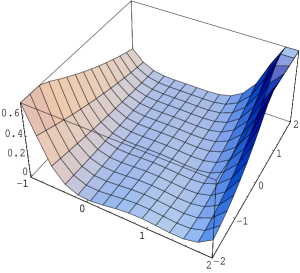
Figure 2: The potential $V(f,g)$ for $j=3/2$.

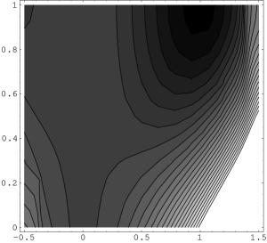
Figure 3: Contour plot of $V(f,h)$ for $j=3/2$.

It is clear from Fig (3) that it is possible to roll down reducible representations $\tilde{J}_{i}$ (the point $f=h=0$) to the irreducible representation $J_{i}$ (the point $f=h=1$) without experiencing an energy barrier.

In [34], we develop a geometrical picutre of this dynamical process, where two spheres merge into one through non-spherical deformations.

To conclude this section, we have shown that within the ansatz (6.5) it is possible to roll down from a reducible representation to an irreducilbe representation.

7 Effect of adding a mass term

In this section we present briefly the effect of adding mass terms to our model (2.1):

$$S=T_{0}\int dt{\rm Tr}({1\over 2}\dot{X}_{i}^{2}+\frac{1}{4}[X_{i},X_{j}]^{2}-\frac{2i\kappa}{3}\epsilon_{ijk}X^{i}X^{j}X^{k}-\frac{m^{2}}{2}X_{i}X_{i})$$ (7.1)

The static equation of motion is

$$[X_{j},\bigg{(}[X_{i},X_{j}]-i\kappa\ \epsilon_{ijk}X_{k}\bigg{)}]-m^{2}X_{i}=0.$$ (7.2)

Once again this admits solutions of the form (2.7)

$$X_{i}=a\oplus_{r=1}^{s}J_{i}^{(r)}$$ (7.3)

where now $m^{2}=2(a\kappa-a^{2})$, i.e.

$$a=(\kappa\pm\sqrt{\kappa^{2}-2m^{2}})/2$$ (7.4)

The lower sign gives an unstable solution, so we shall only consider the upper sign henceforth.

The model is supersymmetric for $m=\frac{2\kappa}{3}$ [9]. However, for the time being we will work with generic $m$. In the table below we list the quadratic fluctuation spectrum and the value of the action around (7.3).

Table 3: Fluctuation spectrum with mass term

Solution	$\omega^{2}$	Multiplicity	Action
	0	7
	$m^{2}$	3
$\frac{1}{2}\oplus 0$	$3(\kappa^{2}+3m^{2}+\kappa\sqrt{\kappa^{2}-2m^{2}})/8$	8	$\frac{a^{2}}{4}(3a^{2}-4a\kappa+3m^{2})$
	$(\kappa^{2}+m^{2}+\kappa\sqrt{\kappa^{2}-2m^{2}})$	5
	$\kappa^{2}-2m^{2}+\kappa\sqrt{\kappa^{2}-2m^{2}}$	1
	0	12
$\frac{1}{2}\oplus\frac{1}{2}$	$m^{2}$	9	$\frac{a^{2}}{2}(3a^{2}-4a\kappa+3m^{2})$
	$(\kappa^{2}+m^{2}+\kappa\sqrt{\kappa^{2}-2m^{2}})$	20
	$\kappa^{2}-2m^{2}+\kappa\sqrt{\kappa^{2}-2m^{2}}$	4

It is straightforward to see that we get the original energy spectrum in absence of $m$. On the other hand, when $m=2\kappa/3$ all the solutions have zero energy which is consistent with their being supersymmetric vacua.

Let us rescale the field $X_{i}/\sqrt{2}=Y_{i}$ and substitute it in the energy functional of this modified matrix model

$$E={\rm Tr}\int dt\Big{(}{\dot{Y}_{i}}^{2}-[Y_{i},Y_{j}][Y_{i},Y_{j}]+m^{2}Y_{i}Y_{i}+{2\sqrt{2}i\kappa\over 3}\epsilon_{ijk}Y_{i}[Y_{j},Y_{k}]\big{)}.$$ (7.5)

We can write this in terms of a total square term, a total derivative term and a defect term.

$$E = {\rm Tr}\int dt\left[\dot{Y}_{i}\pm\left({2\sqrt{2}\over 3}\kappa Y_{i}+{i\over 2}\epsilon_{ijk}[Y_{j},Y_{k}]\right)\right]^{2}+{\rm Tr}\int dt(m^{2}-{4\kappa^{2}\over 9})Y_{i}^{2}$$ (7.6)

$$\mp {\rm Tr}\int dt{d\over dt}\left(\left({2\sqrt{2}\over 3}\kappa\right)Y_{i}^{2}+{i\over 3}\epsilon_{ijk}Y_{i}[Y_{j},Y_{k}]\right).$$

Lowest energy configurations are those which equate the first term to zero. This gives us the first order equation. Second term in the energy functional is the defect term. As it stands it is also a total square term but equating it to zero gives us only trivial solution. It is this term which vanishes in the supersymmetric limit, giving rise to the classical form of the Bogomolnyi energy functional. In the Bogomolnyi limit, energy functional factorises into perfect square terms and total derivative terms. While setting former to zero gives us first order equations of motion, latter gives us the energy/mass of the solution. For the time being we will treat the second term in the energy functional as a defect term and will not, either set it to zero or demand it as a constraint on the solution. The first order equations of motion are

$$\dot{Y}_{i}\pm\left({2\sqrt{2}\over 3}\kappa Y_{i}+{i\over 2}\epsilon_{ijk}[Y_{j},Y_{k}]\right)=0.$$ (7.7)

This equation has been studied by Bachas, Hoppe and Pioline[38]. A class of solutions studied by them are those, which interpolate between trivial SU(2) representation and, say, the largest possible irreducible representation of SU(2). The Bachas, Hoppe and Pioline ansatz which solves the equation of motion is

$$Y_{i}={\sqrt{2}\kappa/3\over{1+\exp{(\sqrt{2}\kappa(t-t_{0})/3)}}}\rho_{i}$$ (7.8)

where $\rho_{i}$ is some SU(2) representation. Contribution of the total derivative term to the energy of this configuration comes only from the endpoints of the trajectory, i.e., from difference of the energy of spin 0 representation and that of representation $\rho_{i}$. In addition there is a contribution from the defect term. For the solution under consideration, this defect term contributes infinite energy. Recall that in the supersymmetric limit this defect term vanishes and hence there is no infinite contribution to the energy of this solution. Thus this is a finite energy solution in the supersymmetric problem. Of course, in the supersymmetric case, energy of every vacuum configuration is zero, and hence this solution interpolates between two degenrate vacua. On the contrary, in the non-supersymmetric case, vacuum configurations have different energy which depends upon their SU(2) labels. It is this non-degeneracy of these vacua which is responsible for the infinite energy of these solutions. For large enough $N$, even in the non-supersymmetric scenario, we have degenerate vacua which are labelled by different set of SU(2) indices. If we consider a solution interpolating between these vacua, it will clearly have finite energy.

One of the important implications of the mass term is that the moduli are lifted. This is evident from the first order equations. Static solutions to these equations do not allow the marginal deformations that we studied in section 4. Thus, it is not classically possible any more to roll down from a reducible representation to an irreducible one. Only way we can reach the irreducible representation is by tunneling. The solution discussed above falls in this class.

8 Comments on SUGRA duals

8.1 Polchinski-Strassler scenario

The matrix model (7.1) coincides with the space-independent part of the action for the adjoint scalars of the four-dimensional gauge theory considered in [9]. The supersymmetric point $m=2\kappa/3$ and its SUGRA dual is discussed there in great detail. For other values of $m$, supersymmetry is broken; SUGRA dual of these theories also are briefly mentioned in [9]. Essentially the SUGRA duals of the classical solutions (7.3) of the gauge theory are a collection of 5-branes in a space which is asymptotically $AdS_{5}\times S^{5}$. Close to themselves, the 5-brane world-volume is like $R^{3}\times S^{2}$. The radii of the 2-spheres and their location in the AdS geometry depends on the dimensionality of the representation $J_{i}^{(r)}$ in (7.3).

[9] has indicated a phase diagram in the $(m^{2},\kappa)$ plane where the $m^{2}<0$ represents a phase in which only the irreducible representations are stable. The phase $m^{2}>0$, on the other hand, is qualitatively similar to the supersymmetric point $m=\frac{2\kappa}{3}$; in this phase the reducible representations are all stable. The matrix model (2.1) which we began with has $m^{2}=0$; as we found in our stability analysis, here the reducible representations are marginally stable, with classical instabilities in the cubic order. In terms of the SUGRA dual, this implies that the collection of 5-branes corresponding to the reducible representations should have a mild classical instability towards forming a large 5-brane corresponding to the irredicuble representation.

8.2 F1-NS5 brane system

Another place where this matrix model is relevant is in the F1-NS5 brane system in type IIA string theory. Easiest way to see this is to start with the D1-D5 system of type IIB string theory. The Chern-Simon term on the common worldvolume of the D1-D5 system contains a term ($a,b=0,1$ are common world volume indices, $i,j,k,...=2,3,4,5$ are five-brane directions, transverse directions ignored),

$$S_{cs,D1D5}=\int d^{2}\sigma[\cdots+i{\lambda\over 2}(C^{(4)}_{abij}[\Phi^{j},\Phi^{i}]+C^{(4)}_{aijk}D_{b}\Phi^{i}[\Phi^{k},\Phi^{j}])+\cdots]$$ (8.1)

where we have ignored terms involving higher form potentials. Since the potential $C^{(4)}$ is invariant under S-duality transformation, identical term exists on the common world volume of F1-NS5 brane system in type IIB string theory.

$$S_{cs,NS}=\int d^{2}\sigma[\cdots+i{\lambda\over 2}(C^{(4)}_{abij}[\Phi^{j},\Phi^{i}]+C^{(4)}_{aijk}D_{b}\Phi^{i}[\Phi^{k},\Phi^{j}])+\cdots]$$ (8.2)

Relevant type IIA configuration of F1-NS5 branes is obtained by performing T-duality along the F1 string direction. Suppose F1 string is along $x^{1}$ then, T-duality along $x^{1}$, leads to a term with $C^{(3)}_{tij}$, which comes from $C^{(4)}_{abij}$ and a term with $C^{(3)}_{ijk}$, which comes from $C^{(4)}_{aijk}$. Incorporating these effects of T-duality into (8.2), we see that the common worldvolume theory of F1-NS5 system in type IIA string theory contains the matrix model under consideration. The commutator square term comes from the DBI part of the action. To be able to do T-duality along the F1 direction, i.e. $x^{1}$, we require all the fields (NS-NS as well as R-R) to be independent of $x^{1}$. Therefore, effective common world volume dynamics essentially reduces down to time evolution only. Hence, this situation is identical to the D0 brane system.

9 Summary

Matrix model in the RR four form background has fuzzy spheres as classical solutions demonstrated by Myers[4]. In this paper we studied the energy landscape of these calssical vacua. Contrary to our expectation we found that the reducible SU(2) representations, corresponding to multiple fuzzy sphere solutions are all stable. That is, quadratic fluctuations around these solutions do not have tachyonic instability although these solutions all have higher energy the the irreducible representation. We resolve this puzzle by showing that the equations of motion allows many more solutions. These new solutions are energetically degenerate with the known solutions,viz. SU(2) representations. In other words, original solutions have a large moduli space. Quadratic fluctuations around the new deformed solutions do have tachyonic instability indicating the roll down path towards more stable configurations. The irreducible representation of SU(2) has no nontrivial flat direction as well as the quadratic fluctuation does not have any tachyonic modes. This feature is expected as the irreducible representation is the lowest energy solution. We then compared our results with other approaches, particularly the spherical D2 brane of Bachas, Douglas and Schweigert[6], WZW matrix model of Alekseev, Recknagel and Schomerus[12], and Myers dual D2 brane in the presence of RR four form flux.

We then discussed the effect of marginal deformation and studied the dynamical trajectory which showed that it is classically possible to roll down from a configuration corresponding to a reducible representation to an irreducible representation. We also studied the effect of switching on the mass term in the matrix model. For a specific value of this mass perturbation, the matrix model becomes supersymmetric. At this point all the classical vacua become degenerate with zero energy. Precisely at this point the second order differential equation of motion can be factored into a first order equation. The main new observation in this case is that the moduli are lifted due to mass perturbation. Thus, it is not classically possible any more to roll down from a reducible representation to an irreducible one. However, time dependent solutions to the equation of motion do exist. These tunneling solutions non-perturbatively interpolate between different vacua.

There are several leads which are worth pursuing. Firstly, full time-development of the roll down solution in the massless case is important particularly from the viewpoint of cosmology. Along the same lines it will be interesting to develop the time-dependent solution in supergravity (cf. Sec. 8). Secondly, there is an interesting issue related to topology change due to non-commutativity. In the massless case, there is a topology change classically[34]. On the other hand, in the massive case, there is no classical path interpolating between different classical vacua and therefore, there is no topology change classically, but it can occur via quantum tunnelling [39].

Acknowledgement: We would like to acknowledge discussions with Sumit Das, Shiraz Minwalla and Sandip Trivedi.

Appendix A Eigenvalues

In this appendix, we calculate the eigenvalues $\kappa^{2}\omega^{2}$ of the quadratic fluctuation matrix $M$ in (3.1) around the general, static classical solution (4.1). We present the calculations for $n\times n$ matrices for $n=2,3,4,5$.

N=2
Solution	$\omega^{2}$	Multiplicity
$0\oplus 0$	0	5
	$4(\pm c+c^{2})$	2(each)
$1/2$	0	3
	2	6

Here $\vec{c}$ is the separation between the zero branes, i.e the solution is $X_{i}=c_{i}\sigma_{3}$.

N=3
Solution	$\omega^{2}$	Multiplicity
	0	12
	$4(\pm c+c^{2})$	2 (each)
$0\oplus 0\oplus 0$	$|\vec{c}-\vec{d}|^{2}\pm 2|\vec{c}-\vec{d}|$	2 (each)
	$|\vec{c}+\vec{d}|^{2}\pm 2|\vec{c}+\vec{d}|$	2 (each)
	0	10
$\frac{1}{2}\oplus 0$	2	6
	$\frac{3}{4}(1+4|\vec{c}|^{2}\pm 4\sqrt{3}|\vec{c}|)$	2 (each)
	$\frac{1}{4}(3+12|\vec{c}|^{2}\pm 4\sqrt{3}|\vec{c}|)$	2 (each)
	0	8
$1$	2	6
	6	10

The solution in the 3 0-branes case, is defined as follows:

$X_{i}=c_{i}\lambda_{3}+\frac{d_{i}}{\sqrt{3}}\lambda_{8}$,

where the $\lambda_{3,8}$’s are the Cartan elements.

In the spin $1/2+0$-brane case, the solution is

$X_{i}=\lambda_{i}+c_{i}\lambda_{8}$,

where the $\lambda_{i}$ are non-zero only in the upper left $2\times 2$ block, and form an su(2) sub-algebra.

N=4
Solution	$\omega^{2}$	Multiplicity
	0	19
	2	6
$\frac{1}{2}\oplus 0\oplus 0$	$\frac{3}{4}(1\pm 4\sqrt{3}c+4c^{2})$	2 (each)
	$\frac{1}{4}(3\pm 4\sqrt{3}c+12c^{2})$	2 (each)
	$\frac{4}{3}(\|\vec{\alpha}\|^{2}\pm\sqrt{3}\|\vec{\alpha}\|)$	2 (each)
	$e_{2}$	2 (each)
	0	17
	2	12
$\frac{1}{2}\oplus\frac{1}{2}$	$4(\pm c+c^{2})$	2 (each)
	$2(1\pm 4c+2c^{2})$	2 (each)
	$2(1\pm 2c+2c^{2})$	2 (each)
	$2(1+2c^{2})$	4
	0	17
	2	6
	6	10
$1\oplus 0$	$\frac{2}{3}(3\pm 2\sqrt{6}c+4c^{2})$	2 (each)
	$\frac{2}{3}(3\pm 4\sqrt{6}c+4c^{2})$	2 (each)
	$\frac{2}{3}(3+4c^{2})$	4
	0	15
$\frac{3}{2}$	2	6
	6	10
	12	14

$\|\vec{\alpha}\|^{2}=|\vec{c}|^{2}+2|\vec{d}|^{2}-2\sqrt{2}\vec{c}\cdot\vec{d}\equiv c^{2}+d^{2}-2\sqrt{2}cd$.

$e_{2}=(1/12)(9+4(c+2\sqrt{2}d)^{2}\pm 4\sqrt{3}(c+2\sqrt{2}d)\pm 8\sqrt{3}(c+2\sqrt{2}d))$.

The solution in the spin $1/2+2$ 0-branes case, is defined as follows: $X_{i}=\lambda_{i}+\vec{c}\lambda_{8}+\vec{d}\lambda_{15}$,

where $\lambda_{i}$ are the spin-$1/2$ rotation generators in the upper left $2\times 2$ block (and zero in the rest) and $\lambda_{8}$ and $\lambda_{15}$ are the Cartan generators which are equal to identity in the upper left $2\times 2$ block. This situation represents an $S^{2}$ brane at the origin and two D0-branes located at positions labelled by $\vec{c}$ and $\vec{d}$.

In the spin $1/2+1/2$ case, the two spin half 2-branes are separated along their center of mass by the vector $\vec{c}$, i.e the solution is

$X_{i}=\sigma_{i}\otimes I+c_{i}I\otimes\sigma_{3}$

Similarly, in the spin $1+0-$brane, the solution is

$X_{i}=J_{i}+c_{i}\lambda_{15}$

where $J_{i}$ are the spin-$1$ rotation generators in the upper left $3\times 3$ block, and $\lambda_{15}$ is the Cartan element $(1/\sqrt{6})Diag(1,1,1,-3)$.

N=5
Solution	$\omega^{2}$	Multiplicity
$\frac{1}{2}\oplus 0\oplus$	0	42
$0\oplus 0$	$3/4$	24
	2	6
	0	28
	2	6
	6	10
	$(2/3)(3+4c^{2})$	4
	$(2/3)(3\pm 2\sqrt{6}c+4c^{2})$	2 (each)
$1\oplus 0\oplus 0$	$(2/3)(3\pm 4\sqrt{6}c+4c^{2})$	2 (each)
	$(1/6)(12+|\vec{\beta}|^{2})$	4
	$(1/6)(3|\vec{\gamma}|^{2}\pm 2\sqrt{6\|\vec{\gamma}\|^{2}})$	2 (each)
	$(1/6)(12\pm 2\sqrt{6}|\vec{\beta}|+|\vec{\beta}|^{2})$	2 (each)
	$(1/6)(12\pm 4\sqrt{6}|\vec{\beta}|+|\vec{\beta}|^{2})$	2 (each)
	0	32
$\frac{1}{2}\oplus\frac{1}{2}\oplus 0$	$3/4$	16
	2	24
	0	26
	3/4	8
$\frac{1}{2}\oplus 1$	2	12
	15/4	16
	6	10

$\|\vec{\gamma}\|^{2}=\|\vec{c}\|^{2}+(5/3)\|\vec{d}\|^{2}-2\sqrt{\frac{5}{3}}\vec{c}\cdot\vec{d}$

$\|\vec{\beta}\|^{2}=\|\vec{c}\|^{2}+15\|\vec{d}\|^{2}+2\sqrt{15}\vec{c}\cdot\vec{d}$

and $c=\|\vec{c}\|$.

Note that the solution in the spin $1+2$ 0-branes case, is defined as follows: $X_{i}=\lambda_{i}+\vec{c}\lambda_{21}+\vec{d}\lambda_{24}$, where $\lambda_{i}$ are the spin one rotation generators in the upper left 3X3 block (and zero in the rest) and $\lambda_{21}$ and $\lambda_{24}$ are the Cartan generators which are equal to identity in the upper left 3X3 block. This situation represents an $S^{2}$ brane at the origin and two D0-branes located at positions labelled by $\vec{c}$ and $\vec{d}$.

References

- [1] J. Polchinski, “Dirichlet-branes and Ramond-Ramond Charges,” Phys. Rev. Lett. 75 (1995) 4724 [hep-th/9510017].
- [2] J. Polchinski, “TASI lectures on D-branes,” hep-th/9611050.
- [3] C. V. Johnson, “D-brane primer,” hep-th/0007170.
- [4] R. C. Myers, “Dielectric-branes,” JHEP 9912, 022 (1999) [hep-th/9910053].
- [5] W. I. Taylor and M. Van Raamsdonk, “Multiple Dp-branes in weak background fields,” Nucl. Phys. B 573, 703 (2000) [hep-th/9910052].
- [6] C. Bachas, M. Douglas and C. Schweigert, “Flux stabilization of D-branes,” JHEP 0005, 048 (2000) [hep-th/0003037].
- [7] J. Pawelczyk and S. J. Rey, Phys. Lett. B 493, 395 (2000) [arXiv:hep-th/0007154].
- [8] J. McGreevy, L. Susskind and N. Toumbas, “Invasion of the giant gravitons from anti-de Sitter space,” JHEP 0006, 008 (2000) [hep-th/0003075].
- [9] J. Polchinski and M. J. Strassler, “The string dual of a confining four-dimensional gauge theory,” hep-th/0003136.
- [10] M. Li, “Fuzzy gravitons from uncertain spacetime,” Phys. Rev. D 63, 086002 (2001) [hep-th/0003173].
- [11] J. Pawelczyk, JHEP 0008, 006 (2000) [arXiv:hep-th/0003057].
- [12] A. Y. Alekseev, A. Recknagel and V. Schomerus, “Brane dynamics in background fluxes and non-commutative geometry,” JHEP 0005, 010 (2000) [hep-th/0003187].
- [13] A. Y. Alekseev, A. Recknagel and V. Schomerus, “Open strings and noncommutative geometry of branes on group manifolds,” Mod. Phys. Lett. A 16, 325 (2001) [hep-th/0104054].
- [14] J. Pawelczyk and H. Steinacker, “Matrix description of D-branes on 3-spheres,” arXiv:hep-th/0107265.
- [15] C. V. Johnson, “Enhancons, fuzzy spheres and multi-monopoles,” Phys. Rev. D 63, 065004 (2001) [hep-th/0004068].
- [16] S. P. Trivedi and S. Vaidya, “Fuzzy cosets and their gravity duals,” JHEP 0009, 041 (2000) [hep-th/0007011].
- [17] S. Vaidya, “Perturbative dynamics on fuzzy S**2 and RP**2,” Phys. Lett. B 512, 403 (2001) [hep-th/0102212].
- [18] C. S. Chu, J. Madore and H. Steinacker, JHEP 0108, 038 (2001) [arXiv:hep-th/0106205]
- [19] S. Iso, Y. Kimura, K. Tanaka and K. Wakatsuki, “Noncommutative gauge theory on fuzzy sphere from matrix model,” Nucl. Phys. B 604, 121 (2001) [hep-th/0101102].
- [20] C. V. Johnson, “The enhancon, multimonopoles and fuzzy geometry,” Int. J. Mod. Phys. A 16, 990 (2001) [hep-th/0011008].
- [21] P. Ho, “Fuzzy sphere from matrix model,” JHEP 0012, 015 (2000) [hep-th/0010165].
- [22] S. Bal and H. Takata, “Interaction between two fuzzy spheres,” hep-th/0108002.
- [23] W. I. Taylor, “The M(atrix) model of M-theory,” hep-th/0002016.
- [24] W. Taylor, “M(atrix) theory: Matrix quantum mechanics as a fundamental theory,” Rev. Mod. Phys. 73, 419 (2001) [hep-th/0101126].
- [25] D. Youm, “A note on thermodynamics and holography of moving giant gravitons,” hep-th/0104011.
- [26] J. Y. Kim and Y. S. Myung, “Vibration modes of giant gravitons in the background of dilatonic D-branes,” Phys. Lett. B 509, 157 (2001) [hep-th/0103001].
- [27] A. Mikhailov, “Giant gravitons from holomorphic surfaces,” JHEP 0011, 027 (2000) [hep-th/0010206].
- [28] S. R. Das, A. Jevicki and S. D. Mathur, “Vibration modes of giant gravitons,” Phys. Rev. D 63, 024013 (2001) [hep-th/0009019].
- [29] S. R. Das, S. P. Trivedi and S. Vaidya, “Magnetic moments of branes and giant gravitons,” JHEP 0010, 037 (2000) [hep-th/0008203].
- [30] S. R. Das, A. Jevicki and S. D. Mathur, “Giant gravitons, BPS bounds and noncommutativity,” Phys. Rev. D 63, 044001 (2001) [hep-th/0008088].
- [31] K. Millar, W. Taylor and M. V. Raamsdonk, “D-particle polarizations with multipole moments of higher-dimensional branes,” hep-th/0007157.
- [32] E. Witten, “Noncommutative Geometry And String Field Theory,” Nucl. Phys. B 268, 253 (1986).
- [33] T. Banks, W. Fischler, S. H. Shenker and L. Susskind, “M theory as a matrix model: A conjecture,” Phys. Rev. D 55, 5112 (1997) [hep-th/9610043].
- [34] G. Mandal, S. R. Wadia and K. P. Yogendran, to appear.
- [35] K. Hashimoto and K. Krasnov, “D-brane solutions in non-commutative gauge theory on fuzzy sphere,” Phys. Rev. D 64, 046007 (2001) [arXiv:hep-th/0101145].
- [36] R. Dijkgraaf, E. Verlinde and H. Verlinde, “C = 1 Conformal Field Theories On Riemann Surfaces,” Commun. Math. Phys. 115, 649 (1988).
- [37] J. Gomis, T. Mehen and M. B. Wise, “Quantum field theories with compact noncommutative extra dimensions,” JHEP 0008, 029 (2000) [hep-th/0006160].
- [38] C. Bachas, J. Hoppe and B. Pioline, “Nahm equations, N = 1* domain walls, and D-strings in AdS(5) x S(5),” JHEP 0107, 041 (2001) [hep-th/0007067].
- [39] H. Grosse, M. Maceda, J. Madore and H. Steinacker, “Fuzzy instantons,” arXiv:hep-th/0107068.