The Born-Infeld Sphaleron

Abstract

We study the SU(2) electroweak model in which the standard Yang-Mills coupling is supplemented by a Born-Infeld term. The deformation of the sphaleron and bisphaleron solutions due to the Born-Infeld term is investigated and new branches of solutions are exhibited. Especially, we find a new branch of solutions connecting the Born-Infeld sphaleron to the first solution of the Kerner-Gal’tsov series.

1 Introduction

While in the pure Yang-Mills (YM) theory no particle-like, finite energy solutions are possible, they might exist as soon as scale invariance breaking terms appear in the Lagrangian. These can be of different types. The possibility discovered first is the coupling of the YM system to a scalar Higgs field. This breaks the scale invariance and particle-like solutions exist: a) monopoles [1], when the Higgs field is given in the adjoint representation of $SU(2)$ and b) sphalerons [2], when the Higgs field is given in the fundamental representation of $SU(2)$. While these solutions were studied extensively since their discovery, the coupling of gravity to YM theories was rather neglected. It was believed that gravity was to weak to have important effects on these solutions. The interest only rose when Bartnik and McKinnon [16] found a particle-like, finite energy solution of the coupled Einstein-YM system.

Recently, it was discovered that superstring theory induces important modifications for the standard quadratic YM action. Likely the relevant effective action is of the Born-Infeld type [4] and, naturally, a scale invariance breaking term is involved. This was exploited to construct classical ”glueballs” in the SU(2) Born-Infeld theory [5].

Considering the classical equations of non-abelian field theories coupled to various other fields leads - depending on the coupling constants - in general to a rich pattern of solutions involving several branches related by bifurcations and/or connected by catastrophe-like cusps [6, 7, 8].

In this paper we investigate the effect of a Born-Infeld term on the sphaleron and bisphaleron solutions arising in the SU(2) part of the electroweak model and we find that these solutions are smoothly deformed up to a critical value of the Born-Infeld parameter $\beta_{BI}^{2}$. From there, another branch of solution exists which connects the sphaleron branch to the first solution of the series obtained in [5], while the bisphaleron branch bifurcates with the sphaleron branch at a value of $\beta_{BI}^{2}$ depending on the Higgs mass.

The model, the notations and the ansatz are given in Sect. 2, we discuss some special limiting solutions in Sect. 3 and present and discuss our numerical results in Sect. 4. Finally, in Sect. 5 we comment on the stability of the solutions.

2 SU(2) Born-Infeld-Yang-Mills-Higgs (BIYMH) theory

Neglecting the $U(1)$ part (for technical reasons), we consider the Lagrangian of the SU(2) part of the electroweak model in which the term of the Lagrangian containing the field strength of the Yang-Mills (YM) fields is replaced by the corresponding Born-Infeld (BI) term. The Lagrangian density reads

$${\cal L}=\beta_{BI}^{2}(1-R)+D_{\mu}\phi^{+}D^{\mu}\phi-{\lambda\over 4}(\phi^{+}\phi-{v^{2}\over 2})^{2}$$ (1)

$$R=(1+{1\over{2\beta_{BI}^{2}}}F^{a}_{\mu\nu}F^{a\mu\nu}-{1\over{16\beta_{BI}^{4}}}(F^{a}_{\mu\nu}\tilde{F}^{a\mu\nu})^{2})^{1\over 2}$$ (2)

where $\beta_{BI}$ is the coupling of the BI term and has dimension $L^{-2}$. In the limit $\beta_{BI}^{2}\rightarrow\infty$, the standard $SU(2)$ electroweak Lagrangian is recovered. We study classical, spherically symmetric, static solutions with finite energy $E(\beta_{BI}^{2},v^{2},\lambda)$. A suitable rescaling of the space variable $\vec{x}$ leads to a rescaling of the energy as follows :

$$E(\beta_{BI}^{2},v^{2},\lambda) = vE({\beta_{BI}^{2}\over{v^{4}}},1,\lambda)$$ (3)

$$= \sqrt{\beta_{BI}}E(1,{v^{2}\over{\beta_{BI}}},\lambda)$$ (4)

We are using the standard spherically symmetric ansatz of [6, 7]

$$A^{a}_{0} = 0$$

$$A_{i}^{a} = \frac{1-f_{A}(r)}{gr}\epsilon_{aij}\hat{x}_{j}+\frac{f_{B}(r)}{gr}(\delta_{ia}-\hat{x}_{i}\hat{x}_{a})+\frac{f_{C}(r)}{gr}\hat{x}_{i}\hat{x}_{a}$$

$$\phi = \frac{v}{\sqrt{2}}\bigl{[}H(r)+iK(r)(\hat{x}^{a}\sigma_{a})\bigr{]}\left(\begin{array}[]{c}0\\ 1\end{array}\right)$$ (7)

where $f_{A}(r)$, $f_{B}(r)$, $f_{C}(r)$, $H(r)$ and $K(r)$ are functions of the radial coordinate $r$ only and $\hat{x}_{a}\equiv r_{a}/r$. It is well known (see e.g. [6, 7, 9]) that this ansatz is plagued with a residual gauge symmetry, which we will fix here by imposing the axial gauge :

$$x^{i}A_{i}=0\ \ \ \Rightarrow\ \ \ f_{C}(r)=0\ \ .$$ (8)

Since we consider static solutions here and due to the choice $A^{a}_{0}=0$, the term including the dual field strength tensor in (2) vanishes. The masses of the gauge boson and Higgs boson, respectively, are given by:

$$M_{W}={1\over 2}gv\ ,\ M_{H}=\sqrt{\lambda}v$$ (9)

With the rescaling

$$x=M_{W}r$$ (10)

the energy $E$ depends only on two fundamental couplings

$$\beta^{2}\equiv{\beta_{BI}^{2}\over{(M_{W})^{4}}}=16{\beta_{BI}^{2}\over{g^{4}v^{4}}}\ ,\ \epsilon\equiv{1\over 2}({M_{H}\over{M_{W}}})^{2}=2{\lambda\over{g^{2}}}$$ (11)

and is given as 1-dimensional integral over the energy density ${\cal E}$ (the prime denotes the derivative with respect to $x$):

$$E(\beta^{2},\epsilon)={4\pi\over{g^{2}}}M_{W}\int dx\ {\cal E},$$ (12)

$${\cal E} = \beta^{2}x^{2}\left(\sqrt{1+{1\over{\beta^{2}x^{2}}}(2(f^{{}^{\prime}2}_{A}+f^{{}^{\prime}2}_{B}+({f^{2}_{A}+f^{2}_{B}-1\over x})^{2})}-1\right)$$ (13)

$$+ (K(f_{A}+1)+HF_{B})^{2}+(H(F_{A}-1)-Kf_{B})^{2}+2x^{2}(H^{{}^{\prime}2}+K^{{}^{\prime}2})$$

$$+ \epsilon x^{2}(H^{2}+K^{2}-1)^{2}$$

The corresponding Euler-Lagrange equations can be obtained in a straighforward way and have to be solved with respect to specific boundary conditions which are necessary for the solution to be regular and of finite energy. In [6, 7] it was found that two possible sets of boundary conditions exist. After an algebra, it can be shown that these two sets of conditions also hold when the Yang-Mills part of the action is replaced by the Born-Infeld term. The first of these sets was used to construct the solution of [2]. Two of the radial functions vanish identically : $f_{B}(x)=H(x)=0$ and the other two have to obey

$$f_{A}(0)=1\ \ f_{A}(\infty)=-1$$ ,

$$K(0)=0\ \ K(\infty)=1$$ , (14)

For the second set, all functions are non-trivial and their boundary conditions at the origin read :

$$f_{A}(0)=1\ \ \ \ ,\ \ \ \ f_{B}(0)=0$$ (15)

$$H^{\prime}(0)=0\ \ \ \ ,\ \ \ \ K(0)=0$$

while in the limit $x\rightarrow\infty$, the functions have to approach constants in the following way

$${\rm lim}_{x\rightarrow\infty}(f_{A}(x)+if_{B}(x)) ={\rm exp}(2i\pi q)$$ (16)

$${\rm lim}_{x\rightarrow\infty}(H(x)+iK(x)) ={\rm exp}(i\pi q)$$

The solutions of this second type are thus characterized by a real constant $q\in[0,1[$. This parameter has to be determined numerically and depends on $\epsilon$ and $\beta$.

3 Limiting Solutions

Two parameter limits of the model studied here are of special interest and have been studied previously:

a)

$\beta_{BI}^{2}=\infty$.
In this limit, the standard $SU(2)$ electroweak Lagrangian is obtained. Classical, finite energy solutions were found for the two different sets of boundary conditions discussed above. The case in which $f_{B}$ and $H$ vanish is the sphaleron discovered by Klinkhamer and Manton [2]. It has energy of the form

$$E_{sp}={M_{W}\over{\alpha_{W}}}\ I(\epsilon)\quad,\quad\alpha_{W}={4\pi\over{g^{2}}}$$ (17)

where $I(\epsilon)$ has to be determined numerically. It was found that [2, 10]

$$I(0)\simeq 3.04\ ,\ I(0.5)\simeq 3.64\ ,\ I(\infty)\simeq 5.41$$ (18)

For sufficiently large values of $\epsilon$ (i. e. $\epsilon>\epsilon_{cr}\approx 72$) solutions of the second type appear [6, 7] : the bisphalerons which occur as a pair of solutions related by a parity operation. Their classical energy is lower than the energy of the sphaleron (e.g. $I_{bi}(\epsilon=\infty)\approx 5.07$). In the limit $\epsilon\rightarrow\epsilon_{cr}$ the functions describing the bisphaleron converge in an uniform way to the functions of the corresponding sphaleron.

b)

$v=0$.
In this case the Higgs field decouples and we are left with the pure SU(2) Born-Infeld theory which was studied recently in [5]. While the pure YM system does not admit finite energy solutions, the presence of the BI term breaks the scale invariance and finite energy solutions, so-called ”glueballs” exist. These are indexed by the number $n$ of nodes of the function $f_{A}^{(n)}(r)$. The first element of the sequence, $f_{A}^{(1)}(r)$, has exactly one node and with the convention adopted in [5] the energy (in units of $4\pi$) is given by

$$E_{KG}=E(1,0,0)\equiv M$$ (19)

It was found [5] that for the first solution of the sequence $M\simeq 1.13559$.

4 Numerical results

We have studied numerically the classical equations for several values of the parameters $\beta_{BI}^{2},v,\lambda$. By taking advantage of the scaling (3), (4) we fixed $v=1$ without loosing generality. These solutions are therefore essentially characterized by the classical energy $E(\beta_{BI}^{2},1,\lambda)=E(\beta^{2},\epsilon)$.

4.1 BI-sphaleron

Starting from the sphaleron solution ($\beta^{2}=\infty$) we constructed a branch of smoothly deformed solutions up to a critical value $\beta^{2}=\beta^{2}_{c}$ along which the energy slightly decreases. $\beta^{2}_{c}$ depends on $\epsilon$ and is increasing for increasing $\epsilon$ which is demonstrated in the following table:

$\epsilon$	0.5	1	2	10	100	200
$\beta^{2}_{c}$	26.5	37.4	39.7	65.0	110.	121.

No solution seems to exist for $\beta^{2}<\beta^{2}_{c}$, but we obtain strong numerical evidence that a second branch of solution exist for $\beta^{2}\in[\infty,\beta^{2}_{c}]$. For fixed $\beta^{2}$, the energy of the solution of this second branch is higher than the energy of the one of the first branch. We therefore refer to these branches as to the lower and upper branch, respectively. For the upper branch we find

$$\lim_{\beta^{2}\rightarrow\infty}E(\beta^{2},\epsilon)=\infty$$ (20)

This can be understood as follows: on the lower branch, $\beta^{2}\rightarrow\infty$ corresponds to $v$ fixed and non-equal zero with $\beta_{BI}^{2}\rightarrow\infty$, while on the upper branch this limit corresponds to $\beta_{BI}^{2}$ fixed and $v\rightarrow 0$. Because of the special choice of the coordinates (10), the solution on the upper branch shrinks to zero (see also Fig. 4), while its energy tends to infinity for $\beta^{2}\rightarrow\infty$. With an appropriate rescaling $E(\beta^{2},\epsilon)$ $\rightarrow$ $(\beta)^{-{1\over 2}}E(\beta^{2},\epsilon)$ the mass of the $n=1$ Kerner-Galtsov solution is recovered

$$M=\lim_{\beta\rightarrow\infty}\beta^{-{1\over 2}}E(\beta^{2},\epsilon)$$ (21)

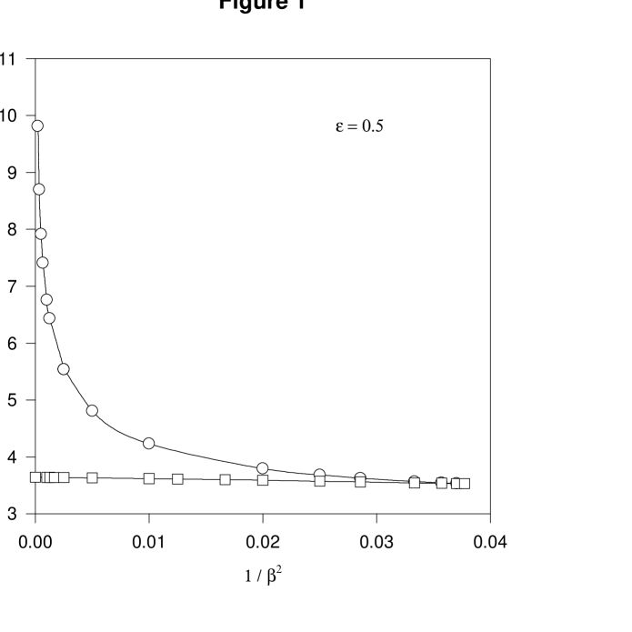
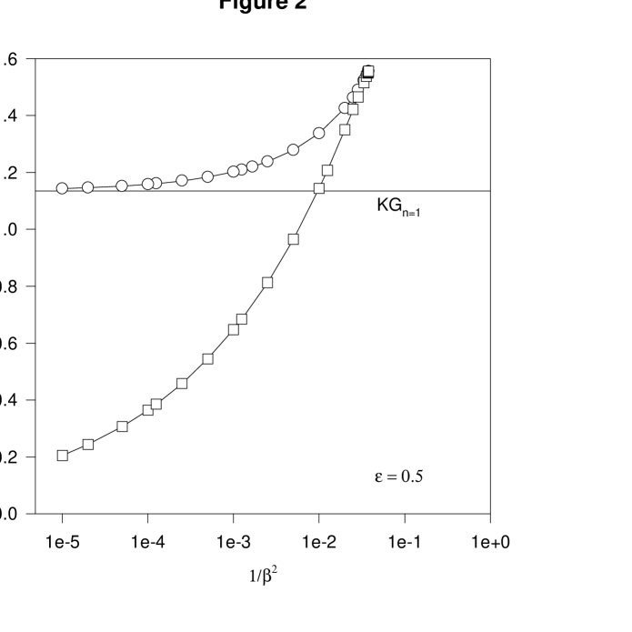
For $\epsilon=0.5$, the energy of the solutions on both branches before the rescaling is illustrated in Fig. 1, the energy after the rescaling in Fig. 2.

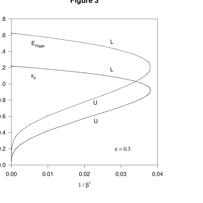
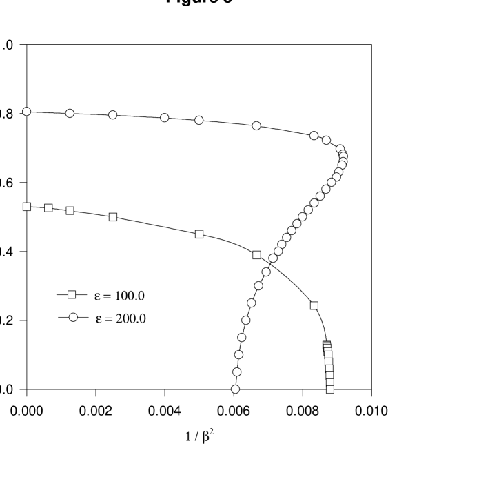
In Fig. 3 we show the value $x_{0}$ of the radial coordinate $x$, for which $f_{A}^{(1)}$ attains its node. Clearly, this value tends to zero for $\beta^{2}\rightarrow\infty$ on the upper branch. As already mentioned this is due to the fact that the rescaled variable $x$ shrinks to zero for $v\rightarrow 0$. Also shown in Fig. 3 is the contribution $E_{Higgs}$ of the Higgs field energy to the total energy of the solution. While on the lower branch it stays finite for all values of $\beta^{2}$, it tends to zero on the upper branch for $\beta^{2}\rightarrow\infty$ . This supports the interpretation that on the upper branch the Higgs field is trivial for $\beta^{2}=\infty$.

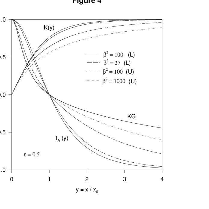
Finally, we demonstrate the convergence of the $n=1$-solution to the corresponding Kerner-Gal’tsov (KG) solution for $\epsilon=0.5$ in Fig. 4. The profiles of the gauge field and Higgs field functions are shown on the lower branch for $\beta^{2}=100$ and a value $\beta^{2}=27$ close to the critical $\beta^{2}_{c}$. Clearly, the functions tend to that of the KG solution on the upper branch for increasing $\beta^{2}$. In the limit $\beta^{2}\rightarrow\infty$, $f_{A}$ tends to the gauge field function of the KG solution, while the Higgs field function $K$ tends to zero on the full intervall $[0:\infty[$.

4.2 BI-bisphaleron

For sufficiently high value of the Higgs-boson mass (i.e. for $\epsilon>72$) bisphaleron solutions can be constructed. As in the case of the sphaleron, bisphalerons are smoothly deformed by the Born-Infeld parameter. By studying these solutions in detail for $\epsilon=100$ and $\epsilon=200$ and varying $\beta^{2}$, we observed that like the BI-sphalerons the deformed bisphalerons exist up to a critical value $\beta^{2}=\tilde{\beta}_{c}^{2}$. For $\epsilon=100$, the BI-bisphaleron branch merges into the lower BI-sphaleron branch at $\beta^{2}=\tilde{\beta}_{c}^{2}$. For still higher values of $\epsilon$ the pattern is slightly different. Another branch of BI-bisphaleron exist on the interval $\beta\in[\tilde{\beta}_{c}^{2},\hat{\beta}^{2}]$ and the solutions on this branch merge into the upper BI-sphaleron branch in the limit $\beta^{2}\rightarrow\hat{\beta}^{2}$. In both cases, all radial functions characterizing the BI-bisphaleron converge in an uniform way to the radial functions associated with the corresponding BI-sphaleron. These various phenomena are illustrated in Fig. 5 where the value $H(0)\propto|\phi(0)|$ is shown as function of $1/\beta^{2}$ for $\epsilon=100$ and $\epsilon=200$. For $\epsilon=100$, this quantity clearly tends to zero for $\tilde{\beta}_{c}^{2}=\hat{\beta}^{2}\approx 113.6$. For $\epsilon=200$, we find that $\tilde{\beta}_{c}^{2}\approx 108.8$ (with $H(0)\neq 0$), while the bisphaleron bifurcates with the sphaleron (with $H(0)$ tending to zero) at $\hat{\beta}^{2}\approx 164$. We further observed that for fixed $\beta^{2}$ and for both lower and upper branches, the energy of the BI-bisphaleron is close, although lower, than the energy of the BI-sphaleron. In the limit $\beta^{2}\rightarrow\hat{\beta}^{2}$, the two upper branches (if any) merge into a single one corresponding to the BI-sphaleron upper branch.

5 Stability

Let us finally discuss the (in)stability of our solutions. When two branches of solutions do exist terminating into a catastrophe spike, like the ones shown in Figs. 1 and 2, it is widely believed that the number of negative modes is constant along each branch and that the number of negative modes on the branch with higher energy exceeds the number of negative modes on the branch with lower energy by one unit. The reasoning is based on catastrophe theory [12] and was demonstrated to hold in the context of classical solutions in various models (e.g. [8, 11]).

For $\epsilon<72$, the lower branch corresponds to the deformed electroweak sphaleron and thus possesses a single direction of instability. Therefore, the solutions on the lowest branch likely have one direction of instability while the solutions on the upper branch possess two. This is not in contradiction with the result of [5] because these solutions, when embedded into a field theory with extra fields (here the Higgs field), likely acquire extra unstable modes due to the supplementary degrees of freedom.

For the values of $\epsilon>72$ we have considered here, the bisphaleron possesses one direction of instability on the lower branch while the sphaleron has two. On its upper branch (i.e. for $\hat{\beta}^{2}\geq\beta^{2}\geq\tilde{\beta}_{c}^{2}$) the BI-bisphaleron (resp. BI-sphaleron) possesses two (resp. three) directions of instability. For $\beta^{2}\geq\hat{\beta}^{2}$ only the upper branch of the BI-sphaleron exists and it likely possesses two unstable modes, similarly to the case $\epsilon<72$.

Finally, for $\epsilon>9500$ the situation is still more involved [6, 7]. Nevertheless, the BI-bisphaleron possesses a single direction of instability on its lower branch and the above conclusions should apply, too.

6 Summary

We have studied the Born-Infeld deformation of the SU(2) electroweak sphaleron and bisphaleron. We find that the solutions exist up to a critical value of the Born-Infeld coupling $\beta_{c}^{2}$ (resp. $\tilde{\beta}_{c}^{2}$) which depends on the Higgs mass parameter.

The fact that classical solutions of Born-Infeld like gauge field theories cease to exist at a critical value of the parameter $\beta^{2}$ was observed in several models with Abelian [13] and non-Abelian [14, 15] gauge groups. Especially for the case of BI-vortices, it was shown recently [16] that the magnetic field $B(0)$ of the solution becomes infinite when the critical value $\beta_{c}^{2}$ is approached.

The situation here is slightly different. Indeed, the solutions exist only for $\beta^{2}>\beta_{c}^{2}$, but we constructed numerically a second branch of solutions existing up to $\beta^{2}=\infty$. There the solution tends to the first solution of the KG series and - after an appropriate rescaling - the energy on this upper branch reaches the mass of the $n=1$ KG solution in the limit $\beta^{2}\rightarrow\infty$. When BI-bisphaleron are present, the pattern is qualitatively similar: the BI-bisphaleron branch bifurcates from one of the BI-sphaleron branches (upper or lower, depending of the value of $\epsilon$). No BI-bisphalerons exist as an upper branch for sufficiently high values of $\beta^{2}$.

Sphaleron solutions can also be studied in models where the Born-Infeld term is incorporated by using a symmetrized trace. The result of [17] suggests though, that no qualitative changes of the critical pattern should occur.

Figure 1: The energy $E$ is shown as a function of $1/\beta^{2}$ for $\epsilon=0.5$.

Figure 2: The ratio $E(1/\beta^{2})/\beta^{1\over 2}$ is shown as a function of $1/\beta^{2}$ for $\epsilon=0.5$. The horizontal solid line represents the energy of the $n=1$ KG solution in units of $4\pi$ with $M\simeq 1.135$.

Figure 3: The value $x_{0}$ for which $f_{A}^{(1)}(x_{0})=0$ as well as the contribution $E_{Higgs}$ of the Higgs field energy to the total energy of the solution are plotted as functions of $1/\beta^{2}$ for $\epsilon=0.5$ . The labels $L$ and $U$, respectively, refer to the lower and upper branch.

Figure 4: The profiles of the solutions $(f_{A}^{(1)},K)$ as function of $y=x/x_{0}$ are shown for several values of $\beta^{2}$ and $\epsilon=0.5$. For comparison, the profile of the function $f_{A}^{(1)}$ of the $n=1$ KG solution is also shown. $K(y)\equiv 0$ for the KG solution.

Figure 5: The value $H(0)$ $\propto$ $|\phi(0)|$ characterizing the bisphaleron solution is shown as a function of $1/\beta^{2}$ for two values of $\epsilon$.

References

-
[1]
G. ’t Hooft, Nucl. Phys. B79 (1974) 276;
A. M. Polyakov, JETP Lett. 20 (1974) 194. - [2] F. Klinkhamer and N.S. Manton, Phys. Rev. D30 (1984) 2218.
- [3] R. Bartnik and J. McKinnon, Phys. Rev. Lett. 61 (1988) 141.
- [4] A. Tseytlin, Nucl. Phys. B501 (1997) 41.
- [5] D. Gal’tsov and R. Kerner , Phys. Rev. Lett. 84 (2000) 5955.
- [6] J. Kunz and Y. Brihaye, Phys. Lett. B216 (1989) 253.
- [7] L. Yaffe, Phys. Rev. D40 (1990) 3463.
- [8] Y. Brihaye, J. Kunz and C. Semay, Phys. Rev. D44 (1991) 250.
- [9] T. Akiba, H. Kikuchi and T. Yanagida, Phys. Rev. D38 (1988) 1937.
- [10] Y. Brihaye and J. Kunz, Phys. Rev. D50 (1994) 4175.
- [11] Y. Brihaye and J. Kunz, Phys. Lett. B249 (1990) 90.
- [12] F.V. Kusmartsev, Phys. Rep. C183 (1989) 1.
- [13] E. Moreno, C. Nunez and F. A. Shaposnik, Phys. Rev. D58 (1998) 025015.
- [14] N. Grandi, E. Moreno and F. A. Shaposnik, Phys. Rev. D59 (1999) 125014.
- [15] N. Grandi, R. L. Pakman, F. A. Shaposnik and G. Silva, Phys. Rev. D60 (1999) 125002.
- [16] Y. Brihaye and B. Mercier, Phys. Rev. D64 (2001) 044001.
- [17] V. V. Dyadichev and D.D. V. Galt’sov, Nucl. Phys. B590 (2000) 504.