Local Casimir energy for a wedge with a circular outer boundary

Abstract

The local Casimir energy is investigated for a wedge with and without a circular outer boundary due to the confinement of a massless scalar field with general curvature coupling parameter and satisfying the Dirichlet boundary conditions. Regularization procedure is carried out making use of a variant of the generalized Abel-Plana formula, previously established by one of the authors. The surface divergences in the vacuum expectation values of the energy density near the boundaries are considered. The corresponding results can be applied to the cosmic strings.

1 Introduction

There are two main mechanisms which contribute to the energy of the vacuum: spontaneous symmetry breaking and the Casimir effect. The Casimir effect is a direct consequence of the quantum field theory and it is one of the most interesting macroscopic manifestations of the nontrivial properties of the physical vacuum. Although the Casimir effect has been extensively studied [1, 2, 3, 4] there are still difficulties in both its interpretation and renormalization [3, 5]. Moreover, the absence of a complete renormalization procedure, in practice, limits all calculations to the special case of highly-symmetric boundary configurations (parallel plates, sphere, cylinder) with a specific background metric. From this point of view the wedge with a cylindrical outer boundary is an interesting system, since the geometry is nontrivial and it includes two dynamical parameters, radius and angle, for phenomenological purposes. Due to the formal analogy that exists between a wedge and a straight cosmic string, the corresponding results can be applied to cosmic strings. Cosmic strings predicted in the framework of various gauge theories with spontaneously broken symmetries could have been created at cosmological phase transitions in the early universe [6, 7]. In the case of a static and straightline cosmic string the outside geometry is a locally flat conical spacetime with an angle ’deficit’ $8\pi\mu$ and $\mu$ is the linear mass density of the string. The superconducting strings form a particular subclass of cosmic strings [8]. In the case of scalar field, it is reasonable to impose a Dirichlet boundary condition at $r=a$ [9]. The investigation of the influence of the cosmic strings on the behavior of quantized fields have been carried out in [10]. In this paper we will study the Casimir energy density for a massless scalar field with a general curvature coupling parameter inside a wedge of opening angle $\phi_{0}$ with and without a cylindrical outer boundary assuming the Dirichlet boundary conditions on the constraining surfaces. Some most relevant investigations to the present paper are contained in [11, 12, 2, 13, 14] for a conformally coupled scalar and electromagnetic fields in a four dimensional spacetime. The total Casimir energy of a semi-circular infinite cylindrical shell with perfectly conducting walls is considered in [15] by using the zeta function technique. Our method here employs the mode summation and is based on a variant of the generalized Abel-Plana formula [16] together with an adequate cutoff function. This allows to extract from the vacuum expectation value of the energy density the part due to a wedge without outer cylindrical shell and to present the cylindrical part in terms of the strongly convergent integrosum. We have organized the paper as follows. The next section is devoted to the consideration of the local Casimir energy for a massless scalar field with a general curvature coupling inside a wedge. This investigation generalizes the previously known result for a conformally coupled scalar and is essential for the main purpose of this paper in section 3, where the vacuum densities are considered for a wedge with the outer cylindrical shell. A formula for the shell contribution to the vacuum energy density is derived and the corresponding surface divergences are investigated. Finally, the results are re-mentioned and discussed in section 4.

2 Vacuum energy density inside a wedge for a scalar field with general curvature coupling

In this section we will consider a scalar field $\varphi$, with the curvature coupling parameter $\xi$, obeying Dirichlet boundary condition on the boundary of the wedge-shaped region formed by two plane boundaries intersecting at an arbitrary angle $\phi_{0}$:

$$\phi(t,r,\phi=0,z_{1},\ldots,z_{N})=\phi(t,r,\phi=\phi_{0},z_{1},\ldots,z_{N})=0,$$ (1)

where we use cylindrical coordinates $(r,\phi,z_{1},\ldots,z_{N})$ in $D=N+2$ – dimensional space. The corresponding field equation is in form

$$\left(\nabla^{i}\nabla_{i}+\xi R\right)\varphi(x)=0,$$ (2)

with $R$ being the scalar curvature for the background spacetime. By using this equation, in the case of the flat background the corresponding metric energy-momentum tensor may be presented in the form

$$T_{ik}=\nabla_{i}\varphi\nabla_{k}\varphi+\left[\left(\xi-\frac{1}{4}\right)g_{ik}\nabla^{\mu}\nabla_{\mu}-\xi\nabla_{i}\nabla_{k}\right]\varphi^{2}.$$ (3)

The vacuum expectation values for these quantities can be derived by evaluating the mode sum

$$\langle 0|T_{ik}(x)|0\rangle=\sum_{{\mathbf{\alpha}}}T_{ik}\left\{\varphi_{\mathbf{\alpha}}(x),\varphi_{{\mathbf{\alpha}}}^{\ast}(x)\right\},$$ (4)

where $\{\varphi_{{\mathbf{\alpha}}}(x)\}$ is a complete orthonormal set of positive frequency solutions to the field equation with quantum numbers $\alpha$, satisfying the corresponding boundary conditions. In the region inside the wedge the corresponding eigenfunctions have the form

$$\varphi_{\alpha}(x) = \frac{1}{(2\pi)^{N/2}}\left(\frac{\gamma}{\omega\phi_{0}}\right)^{1/2}J_{l}(\gamma r)\sin(l\phi)\exp\left(i{\mathbf{kr}}_{\parallel}-i\omega t\right),\quad\omega=\sqrt{\gamma^{2}+k^{2}},\quad l=\frac{n\pi}{\phi_{0}},$$ (5)

$$\alpha = (n,\gamma,{\mathbf{k}}),\quad 0<\gamma<\infty,\quad-\infty<k_{j}<\infty,\quad n=1,2,\cdots,$$

where ${\mathbf{r}}_{\parallel}=(z_{1},\ldots,z_{N})$, and $J_{l}(z)$ is the Bessel function. Substituting the eigenfunctions into (4) for the corresponding vacuum energy density one finds

$$\langle 0_{w}|T_{00}|0_{w}\rangle=\frac{1}{2(2\pi)^{N}\phi_{0}}\sum_{n=1}^{\infty}\int_{0}^{\infty}d\gamma\int d^{N}{\mathbf{k}}\frac{\gamma}{\omega}\left[A_{l}^{(-)}\left(\gamma,{\mathbf{k}},r\right)-A_{l}^{(+)}\left(\gamma,{\mathbf{k}},r\right)\cos(2l\phi)\right]$$ (6)

with $|0_{w}\rangle$ being the amplitude for the corresponding vacuum inside a wedge, and we use the notations

$$A_{l}^{(\pm)}\left(\gamma,{\mathbf{k}},r\right)=\omega^{2}J_{l}^{2}(\gamma r)+\left(2\xi-\frac{1}{2}\right)\gamma^{2}\left[\left(1\pm\frac{l^{2}}{\gamma^{2}r^{2}}\right)J_{l}^{2}(\gamma r)-J_{l}^{{}^{\prime}2}(\gamma r)\right].$$ (7)

To evaluate expression (6) firstly we integrate over ${\mathbf{k}}$ by using the formula

$$\int\frac{k^{s}d^{N}{\mathbf{k}}}{\sqrt{k^{2}+\gamma^{2}}}=\gamma^{N+s-1}\frac{\pi^{(N-1)/2}}{\Gamma(N/2)}\Gamma\left(-\frac{N+s-1}{2}\right)\Gamma\left(\frac{N+s}{2}\right),$$ (8)

and next we integrate over $\gamma$ on the base of the formula

$$\int_{0}^{\infty}d\gamma\,\gamma^{\alpha-1}J_{l}^{2}(\gamma r)=\frac{r^{-\alpha}}{2\sqrt{\pi}}\frac{\Gamma\left(\frac{1-\alpha}{2}\right)\Gamma\left(l+\alpha/2\right)}{\Gamma\left(1-\alpha/2\right)\Gamma\left(l+1-\alpha/2\right)}.$$ (9)

The integral involving the derivative of the Bessel function can be evaluated by using the relation

$$\left(1-\frac{l^{2}}{\gamma^{2}r^{2}}\right)J_{l}^{2}(\gamma r)-J_{l}^{{}^{\prime}2}(\gamma r)=-\frac{1}{2\gamma^{2}}\left(\frac{d^{2}}{dr^{2}}+\frac{1}{r}\frac{d}{dr}\right)J_{l}^{2}(\gamma r).$$ (10)

As a result for the separate terms in (6) one finds

$$\int_{0}^{\infty}d\gamma\int d^{N}{\mathbf{k}}\frac{\gamma}{\omega}A_{l}^{(-)}\left(\gamma,{\mathbf{k}},r\right) = \frac{\pi^{N/2-1}}{4r^{N+3}}\Gamma\left(-N/2-1\right)\frac{\Gamma\left(l+\frac{N+1}{2}\right)}{\Gamma\left(l-\frac{N-1}{2}\right)}$$

$$\times\left[(N+1)^{2}(N+2)(\xi-\xi_{c})-l^{2}\right]$$

$$\int_{0}^{\infty}d\gamma\int d^{N}{\mathbf{k}}\frac{\gamma}{\omega}A_{l}^{(+)}\left(\gamma,{\mathbf{k}},r\right)\cos(2l\phi) = \frac{\pi^{N/2-1}}{r^{N+3}}(N+2)(\xi-\xi_{c})\Gamma\left(-N/2-1\right)$$

$$\times\left[\frac{(N+1)^{2}}{4}-l^{2}\right]\frac{\Gamma\left(l+\frac{N+1}{2}\right)}{\Gamma\left(l-\frac{N-1}{2}\right)}\cos(2l\phi),$$

where $\xi_{c}=(D-1)/(4D)$ is the curvature coupling parameter for the conformal case. To obtain the regularized value of the energy density we have to subtract from (6) the corresponding quantity for the Minkowski vacuum without boundaries. The latter can be found in a similar way. The corresponding eigenfunctions are in form

$$\varphi_{\alpha}^{(M)}(x)=\frac{1}{(2\pi)^{(N+1)/2}}\left(\frac{\gamma}{2\omega}\right)^{1/2}J_{n}(\gamma r)\exp\left(in\phi+i{\mathbf{kr}}_{\parallel}-i\omega t\right),\quad n=\cdots-2,-1,0,1,2\ldots.$$ (13)

Now on the base of formula (4) one finds

$$\langle 0_{M}|T_{00}(x)|0_{M}\rangle=\frac{1}{(2\pi)^{N+1}}\sum_{n=0}^{\infty}{}^{\prime}\int_{0}^{\infty}d\gamma\int d^{N}{\mathbf{k}}\frac{\gamma}{\omega}A_{n}^{(-)}\left(\gamma,{\mathbf{k}},r\right),$$ (14)

where $|0_{M}\rangle$ denotes the Minkowski vacuum, and the prime means that in the sum over $n$ the term with $n=0$ is taken with weight $1/2$. Taking into account that $\sum_{n=0}^{\infty}{}^{\prime}J_{n}^{2}(\gamma r)=1/2$ it can be easily seen that expression (14) is presented in the standard form

$$\langle 0_{M}|T_{00}(x)|0_{M}\rangle=\int\frac{d^{D}{\mathbf{k}}}{(2\pi)^{D}}\frac{\omega}{2}.$$ (15)

After integrating over ${\mathbf{k}}$ and $\gamma$ in (14) we receive

$$\langle 0_{M}|T_{00}(x)|0_{M}\rangle=\frac{\Gamma\left(-N/2-1\right)}{2^{N+3}\pi^{N/2+2}r^{N+3}}\sum_{n=0}^{\infty}{}^{\prime}\frac{\Gamma\left(n+\frac{N+1}{2}\right)}{\Gamma\left(n-\frac{N-1}{2}\right)}\left[(N+1)^{2}(N+2)(\xi-\xi_{c})-n^{2}\right].$$ (16)

Let us consider the case $N=1$. The sums over $n$ are evaluated by using the Riemann zeta function $\zeta(s)=\sum_{n=1}^{\infty}n^{-s}$, $\zeta(-1)=-1/12$, $\zeta(-3)=1/120$, and the formula

$$\sum_{n=1}^{\infty}n^{p}\cos(\beta n)=\frac{1}{2}\sin\frac{\pi p}{2}\frac{d^{p}}{d\beta^{p}}\cot(\beta/2),$$ (17)

valid for an odd $p$. For the regularized vacuum energy density this leads

$$\langle T_{00}\rangle_{\mathrm{reg}} = \langle 0_{w}|T_{00}|0_{w}\rangle-\langle 0_{M}|T_{00}|0_{M}\rangle=-\frac{(\pi/\phi_{0})^{4}-1}{1440\pi^{2}r^{4}}-(\xi-\xi_{c})\frac{(\pi/\phi_{0})^{2}-1}{12\pi^{2}r^{4}}+$$ (18)

$$+\frac{\xi-\xi_{c}}{4\phi_{0}^{2}r^{4}}\csc^{2}(\pi\phi/\phi_{0})\left[\frac{\pi^{2}}{2\phi_{0}^{2}}\left(3\csc^{2}(\pi\phi/\phi_{0})-2\right)+1\right],$$

where $\xi_{c}=1/6$ is the curvature coupling parameter for the conformal case in $D=3$. In formula (18) the first two terms on the right come from the summand with $A_{l}^{(-)}\left(\gamma,{\mathbf{k}},r\right)$ in (6), and the last term comes from the summand with $A_{l}^{(+)}\left(\gamma,{\mathbf{k}},r\right)$. For $\phi_{0}=\pi$ it can be easily seen that expression (18) coincides with the well-known result for the Casimir energy density in the case of a single plate geometry. For the conformally coupled case from (18) we obtain the standard result previously derived in Refs. [12],[18]. It is of interest to note that in this case the renormalized energy density is angle independent and is finite on the sides of the wedge. It diverges on the edge as $r^{-4}$ , when $r\rightarrow 0$ (as $r^{-(D+1)}$ for a $D$ – dimensional space). For a non–conformally coupled scalar the energy density is angle dependent and contains surface divergences on the wedge sides. Note that for a minimally coupled scalar ($\xi=0$) the regularized energy density (18) is negative everywhere, $\langle T_{00}\rangle_{\mathrm{reg}}|_{\xi=0}<0$.

3 Vacuum energy density inside a wedge with circular boundary

Having investigated the vacuum energy density inside a wedge we now turn to the case with additional circular boundary with radius $a$. The boundary conditions are Dirichlet ones:

$$\varphi(t,r,\phi=0,z_{1},\ldots,z_{N})=\varphi(t,r,\phi=\phi_{0},z_{1},\ldots,z_{N})=0,$$ (19)

$$\varphi(t,r=a,\phi,z_{1},\ldots,z_{N})=0.$$

The eigenfunctions satisfying these boundary conditions are of the form

$$\varphi_{\alpha}(x)=\beta_{\alpha}J_{l}(\gamma r)\sin(l\phi)\exp\left(i{\mathbf{kr}}_{\parallel}-i\omega t\right),$$ (20)

where the notations are the same as in (5). The normalization coefficient $\beta_{\alpha}$ is determined from the standard Klein-Gordon scalar product and is equal to

$$\beta_{\alpha}^{2}=\frac{2}{(2\pi)^{N}\omega\phi_{0}a^{2}J_{l}^{\prime 2}(\gamma a)}.$$ (21)

The eigenvalues for the quantum number $\gamma$ are quantized by the boundary condition (19) on the cylinder surface $r=a$. From this condition it follows that the possible values of $\gamma$ are equal to

$$\gamma=\lambda_{n,j}/a,\quad j=1,2,\cdots,$$ (22)

where $\lambda_{n,j}$ are positive zeros of the Bessel function, $J_{l}(\lambda_{n,j})=0$, arranged in ascending order, $\lambda_{n,j}<\lambda_{n,j+1}$. Substituting the eigenfunctions (20) into mode sum formula (4) for the corresponding energy density one finds

$$\langle 0|T_{00}|0\rangle=\frac{1}{2}\sum_{n=1}^{\infty}\sum_{j=1}^{\infty}\int d^{N}{\mathbf{k}}\beta_{\alpha}^{2}\left[A_{l}^{(-)}\left(\lambda_{n,j}/a,{\mathbf{k}},r\right)-A_{l}^{(+)}\left(\lambda_{n,j}/a,{\mathbf{k}},r\right)\cos(2l\phi)\right],$$ (23)

with a set of quantum numbers $\alpha=(n,j,{\mathbf{k}})$. The vacuum expectation value (23) is divergent. To make it finite we introduce the cutoff function $\psi_{\mu}(\gamma)$ satisfying the condition $\psi_{\mu}\rightarrow 1$, $\mu\rightarrow 0$. To extract the divergent part we will apply to the sum over $j$ the summation formula [16]

$$\sum_{j=1}^{\infty}\frac{f(\lambda_{n,j})}{\lambda_{n,j}J_{l}^{\prime 2}(\lambda_{n,j})\sqrt{\lambda_{n,j}^{2}+c^{2}}} = \frac{1}{2}\int_{0}^{\infty}\frac{f(z)}{\sqrt{z^{2}+c^{2}}}dz+\frac{\pi}{4}{\mathrm{Res}}_{z=0}\left[\frac{f(z)Y_{l}(z)}{\sqrt{z^{2}+c^{2}}J_{l}(z)}\right]-$$ (24)

$$-\frac{1}{2\pi}\int_{0}^{c}dz\,\frac{K_{l}(z)}{I_{l}(z)}\frac{e^{-l\pi i}f(ze^{\pi i/2})+e^{l\pi i}f(ze^{-\pi i/2})}{\sqrt{c^{2}-z^{2}}}$$

$$+\frac{i}{2\pi}\int_{c}^{\infty}dz\,\frac{K_{l}(z)}{I_{l}(z)}\frac{e^{-l\pi i}f(ze^{\pi i/2})-e^{l\pi i}f(ze^{-\pi i/2})}{\sqrt{z^{2}-c^{2}}},$$

where $Y_{l}(z)$ is the Neumann function, and $I_{l}(z)$, $K_{l}(z)$ are Bessel modified functions. This formula is valid for functions $f(z)$ satisfying the conditions

$$|f(z)|<\epsilon(x)e^{c_{1}|y|},\quad z=x+iy,\quad c_{1}<2,$$ (25)

$$f(z)=o(z^{2|l|-1}),\quad z\rightarrow 0,$$ (26)

where $\epsilon(x)\rightarrow 0$ for $x\rightarrow\infty$.

To evaluate the sum over $j$ in (23) now as a function $f(z)$ we choose

$$f(z)=z\left[A_{l}^{(-)}\left(z/a,{\mathbf{k}},r\right)-A_{l}^{(+)}\left(z/a,{\mathbf{k}},r\right)\cos(2l\phi)\right]\psi_{\mu}(z/a),$$ (27)

assuming a class of cutoff functions for which $f(z)$ satisfies conditions (25) and (26) uniformly with respect to the cutoff parameter $\mu$. It can be seen that the contribution of the first integral on the right of  formula (24) to the energy density (23) corresponds to the energy density for the case of a wedge without outer cylindrical boundary. This quantity was investigated in the previous section. The second and third integrals on the right-hand side of (24) are finite in the limit $\mu\rightarrow 0$. Using the standard formulae for the Bessel function we see that the subintegrand of the second integral is proportional to $\psi_{\mu}(iz/a)-\psi_{\mu}(-iz/a)$. Consequently, after removing the cutoff the contribution of this integral will be zero. Hence, omitting this integral and removing the cutoff for the vacuum energy density we obtain

$$\langle 0|T_{00}|0\rangle = \langle 0_{w}|T_{00}|0_{w}\rangle-\frac{1}{2^{N-1}\pi^{N+1}\phi_{0}a}\sum_{n=1}^{\infty}\int d^{N}{\mathbf{k}}\int_{ka}^{\infty}\frac{zdz}{\sqrt{z^{2}-k^{2}a^{2}}}\frac{K_{l}(z)}{I_{l}(z)}$$ (28)

$$\times\left\{\left[k^{2}I_{l}^{2}(zx)-\left(2\xi-\frac{1}{2}\right)\frac{z^{2}}{a^{2}}\left(I_{l}^{\prime 2}(zx)+I_{l}^{2}(zx)\frac{2\xi+1/2}{2\xi-1/2}\right)\right]\sin^{2}(l\phi)-\right.$$

$$-\left.\left(2\xi-\frac{1}{2}\right)\frac{l^{2}I_{l}^{2}(zx)}{a^{2}x^{2}}\cos^{2}(l\phi)\right\},\quad x=\frac{r}{a}.$$

The integration over ${\mathbf{k}}$ can be done using the formula [19]

$$\int d^{N}{\mathbf{k}}\int_{k}^{\infty}\frac{k^{s}g(z)dz}{\sqrt{z^{2}-k^{2}}}=\frac{\pi^{N/2}}{\Gamma(N/2)}B\left(\frac{N+s}{2},\frac{1}{2}\right)\int_{0}^{\infty}dzz^{N+s-1}g(z),$$ (29)

where $B(x,y)$ is the Euler beta function. As a result for the vacuum energy density (28) one obtains

$$\langle 0|T_{00}|0\rangle=\langle 0_{w}|T_{00}|0_{w}\rangle+\langle T_{00}\rangle_{c},$$ (30)

where $\langle 0_{w}|T_{00}|0_{w}\rangle$ is the vacuum energy density for a wedge without outer cylindrical boundary, and the term

$$\langle T_{00}\rangle_{c}=\frac{4\xi-1}{2^{D-1}\pi^{(D-1)/2}\phi_{0}a^{D+1}\Gamma((D-1)/2)}\sum_{n=1}^{\infty}\int_{0}^{\infty}dz\,z^{D}\frac{K_{l}(z)}{I_{l}(z)}\left[B_{l}^{(-)}\left(zx\right)-B_{l}^{(+)}\left(zx\right)\cos(2l\phi)\right]$$ (31)

is the contribution due to the presence of the cylindrical shell at $r=a$. Here $l$ is defined in accordance with (5) and we have introduced the notations

$$B_{l}^{(\pm)}\left(y\right)=I_{l}^{\prime 2}(y)+I_{l}^{2}(y)\left[1+\frac{2}{(D-1)(4\xi-1)}\mp\frac{l^{2}}{y^{2}}\right].$$ (32)

In accordance with the problem symmetry, expression (31) is invariant under the replacement $\phi\to\phi_{0}-\phi$. Aiming to compare with the result for the energy density of a cylindrical shell with the radius $a$ let us write down the corresponding formula, which is obtained from the general result of [19] and has the form

$$\langle T_{00}\rangle_{{\mathrm{reg}}}^{{\mathrm{cyl}}}=\frac{4\xi-1}{2^{D}\pi^{(D+1)/2}a^{D+1}\Gamma((D-1)/2)}\sum_{n=-\infty}^{+\infty}\int_{0}^{\infty}dz\,z^{D}\frac{K_{n}(z)}{I_{n}(z)}B_{n}^{(-)}\left(zx\right),$$ (33)

with the same notations as in (31).

For $0<r<a$ the cylindrical part (31) is finite for all values $0\leq\phi\leq\phi_{0}$, including the wedge sides. The divergences on these sides are included in the first term on the right-hand side of (30), corresponding to the case without circular boundary. At the edge $r=0$ the boundary part (31) vanishes for $0<\phi_{0}<\pi$, is equal to

$$\langle T_{00}\rangle_{0}|_{r=0}=\frac{4\xi-1}{2^{D}\pi^{(D+1)/2}\Gamma((D-1)/2)a^{D+1}}\int_{0}^{\infty}dzz^{D}\frac{K_{1}(z)}{I_{1}(z)},\quad\phi_{0}=\pi$$ (34)

for $\phi_{0}=\pi$, and diverges as $r^{-2(1-\pi/\phi_{0})}$ for $\phi_{0}>\pi$.

The boundary part $\left\langle T_{00}\right\rangle_{c}$ diverges on the cylindrical surface $r=a$ as well. To investigate the corresponding behavior near this surface let us consider the integrosum in (31), introducing a new integration variable $z\rightarrow lz$:

$${\mathcal{I}}=\sum_{n=1}^{\infty}l^{D+1}\int_{0}^{\infty}dz\,z^{D}\frac{K_{l}(lz)}{I_{l}(lz)}\left[B_{l}^{(-)}\left(lzx\right)-B_{l}^{(+)}\left(lzx\right)\cos(2l\phi)\right].$$ (35)

By taking into account that near the surface $r=a$ main contribution comes from the large values of $l$ we can replace the Bessel modified functions by their uniform asymptotic expansions for large values of the order (see, for instance [17]). In the leading order over $1/l$ one finds

$${\mathcal{I}}=\frac{1}{2x^{2}}\sum_{n=1}^{\infty}l^{D}\int_{0}^{\infty}dz\,z^{D-2}(1+z^{2}x^{2})^{1/2}e^{-2l[\eta(z)-\eta(zx)]}\left[b^{(-)}(zx)-b^{(+)}(zx)\cos(2l\phi)\right],$$ (36)

where

$$b^{(\pm)}(y) = 1+\frac{1}{1+y^{2}}\left[y^{2}\mp 1+\frac{2y^{2}}{(D-1)(4\zeta-1)}\right],$$ (37)

$$\eta(z) = \sqrt{1+z^{2}}+\ln\frac{z}{1+\sqrt{1+z^{2}}}.$$ (38)

Near the cylindrical boundary in the leading order over $1-x$ from (36) we obtain

$${\mathcal{I}}=\frac{1}{2}\left(\frac{\pi}{\phi_{0}}\right)^{D}\sum_{n=1}^{\infty}n^{D}\int_{0}^{\infty}dz\,z^{D-2}(1+z^{2})^{1/2}e^{-2n\pi(1-x)\sqrt{1+z^{2}}/\phi_{0}}\left[b^{(-)}(z)-b^{(+)}(z)\cos(2l\phi)\right].$$ (39)

On the wedge sides $\cos(2l\phi)=1$ and this yields

$${\mathcal{I}}=\left(\frac{\pi}{\phi_{0}}\right)^{D}\sum_{n=1}^{\infty}n^{D}\int_{0}^{\infty}\frac{dz\,z^{D-2}}{(1+z^{2})^{1/2}}e^{-2n\pi(1-x)\sqrt{1+z^{2}}/\phi_{0}},\quad\phi=0,\quad\phi=\phi_{0}.$$ (40)

Summing over $n$ by using

$$\sum_{n=1}^{\infty}n^{D}e^{-\alpha n}=(-1)^{D}\frac{d^{D}}{d\alpha^{D}}\frac{1}{e^{\alpha}-1}\approx\frac{\Gamma(D+1)}{\alpha^{D+1}},\quad\alpha\ll 1$$ (41)

we have

$${\mathcal{I}}=\frac{\phi_{0}\Gamma(D+1)}{2^{D+1}\pi(1-x)^{D+1}}\int_{0}^{\infty}\frac{dz\,z^{D-2}}{\left(1+z^{2}\right)^{D/2+1}}=\frac{\phi_{0}(D-1)\Gamma^{2}\left(\frac{D-1}{2}\right)}{16\pi(1-x)^{D+1}},\quad\phi=0,\quad\phi=\phi_{0}.$$ (42)

Substituting this into formula (31) to the leading order over $(a-r)^{-1}$one finds

$$\langle T_{00}\rangle_{c}\sim\frac{(4\xi-1)\Gamma\left(\frac{D+1}{2}\right)}{2^{D+2}\pi^{(D+1)/2}(a-r)^{D+1}},\quad\phi=0,\phi_{0},\quad r\rightarrow a.$$ (43)

For $D=3$ and a conformally coupled scalar field this term coincides with the first summand on the right of formula (18) with the distance $(a-r)$ from the edge $r=a$, $\phi=0$ (or $\phi=\phi_{0}$) and the opening angle $\pi/2$.

For the angles $0<\phi<\phi_{0}$ by using the formula

$$\sum_{n=1}^{\infty}n^{D}e^{-\alpha n}\cos n\beta=\frac{(-1)^{D}}{2}\frac{d^{D}}{d\alpha^{D}}\left(\frac{\sinh\alpha}{\cosh\alpha-\cos\beta}-1\right),$$ (44)

introducing a new integration variable $y=2\pi(1-x)\sqrt{1+z^{2}}/\phi_{0}$ and expanding over $(1-x)$ one finds that the leading contribution of the term with $b^{(+)}(zx)\cos 2l\phi$ into (36) is equal to

$$\frac{\Gamma(D)}{2^{D+1}(1-x)^{D}}\left[1+\frac{1}{(D-1)(4\xi-1)}\right].$$ (45)

In this case the leading contribution from the term with $b^{(-)}(zx)$ dominates and to the leading order by the way similar to that for (43) one has

$$\langle T_{00}\rangle_{c}\sim\frac{D(\xi-\xi_{c})\Gamma\left(\frac{D+1}{2}\right)}{2^{D}\pi^{(D+1)/2}(a-r)^{D+1}},\quad 0<\phi<\phi_{0},\quad r\rightarrow a.$$ (46)

This leading divergence coincides with the corresponding one for a cylindrical surface of the radius $a$ (see, for instance, [19]).

The surface divergences in the renormalised vacuum expectation values of the local physical observables result from the idealization of the boundaries as perfectly smooth surfaces which are perfect reflectors at all frequencies, and are well known in quantum field theory with boundaries. They are investigated in detail for various types of fields and general shape of smooth boundary [12, 18]. Near the smooth boundary the leading divergence varies as $(D+1)$th power of the distance from the boundary. For conformally invariant fields the coefficient of this leading term is zero. For non-smooth boundaries such as here, the latter is not the case and this leads to the extra divergences in the global quantities such as total Casimir energy (see, for instance, [15] for the case of a semi-circular infinite cylinder and discussion in [20]). It seems plausible that such effects as surface roughness, or the microstructure of the boundary on small scales (the atomic nature of matter for the case of the electromagnetic field [21]) can introduce a physical cutoff needed to produce finite values of surface quantities. An alternative mechanism for introducing a cutoff which removes singular behavior on boundaries is to allow the position of the boundary to undergo quantum fluctuations [22]. Such fluctuations smear out the contribution of the high frequency modes without the need to introduce an explicit high frequency cutoff.

The dependence of the cylindrical boundary part of the vacuum energy density multiplied by $a^{D+1}$, $a^{D+1}\langle T_{00}\rangle_{c}$, on the angle $\phi$ and radial coordinate $x=r/a$ is shown in figure 1 for a minimally coupled scalar ($\xi=0$) and in figure 2 for a conformally coupled scalar ($\xi=\xi_{c}$) in $D=3$. The cases $\phi_{0}=\pi/2$ (left graphics) and $\phi_{0}=\pi/4$ (right graphics) are presented, when the cylindrical part vanishes at the edge $r=0$.

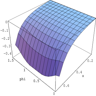
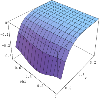
Figure 1: The expectation values for the cylindrical part of the vacuum energy density, $a^{D+1}\langle T_{00}\rangle_{c}$ for $D=3$ minimally coupled scalar field in the cases $\phi_{0}=\pi/2$ (left) and $\phi_{0}=\pi/4$ (right), versus $\phi$ and $x=r/a$.

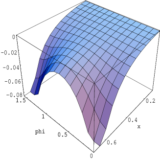
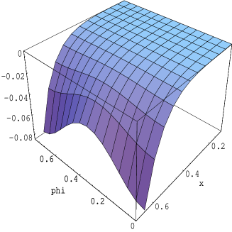
Figure 2: The same as in fig. 1 for a conformally coupled scalar.

4 Final remarks

In the present paper we calculate the vacuum energy density for a massless scalar field with a general curvature coupling and satisfying the Dirichlet boundary conditions in the wedge–shaped region formed by two plane boundaries intersecting at an arbitrary angle $\phi_{0}$ with and without a cylindrical outer boundary. All calculations are made at zero temperature and it is assumed that the boundary conditions are frequency independent. The latter means no dispersive effect is taken into account. The energy density for the wedge, given by formula (18), has been obtained by standard application of the mode summation method. This formula generalizes the result previously known in literature for a conformally invariant scalar field. In the case of a non-conformally coupled scalar the vacuum energy density is angle-dependent and diverges on the wedge sides. For a minimally coupled scalar it is negative everywhere inside a wedge. In the case of presence of an outer cylindrical boundary, discussed in section 3 the expectation value of the corresponding vacuum energy density is presented in the form of series over zeros of the Bessel function. The summation formula for this type of series based on the generalized Abel-Plana formula allows to extract explicitly from the expectation value the part due to the wedge without a cylindrical shell. The additional cylindrical contribution to the vacuum energy density is presented in the form of the strongly convergent integrosum. The latter is finite on the wedge sides but contains surface divergences on the cylindrical boundary. At the edge $r=0$ it vanishes for $0<\phi_{0}<\pi$, is finite for $\phi_{0}=\pi$, and diverges as $r^{-2(1-\pi/\phi_{0})}$ for $\phi_{0}>\pi$. The generalization of the results obtained here for the Neumann, or more general Robin boundary conditions is straightforward. For instance, for the Neumann case in the expressions (5) and (20) of the eigenfunctions the function $\cos(l\phi)$ stands instead of $\sin(l\phi)$ and the quantum number $n$ takes the values $0,1,2,\ldots$. In the case with a circular outer boundary now the eigenvalues for $\gamma a$ are zeros for the derivative of the Bessel function. The formula to sum the series over these zeros can be taken from [16].

References

• [1] Plunien G, Muller B and Greiner W 1986 Phys. Rep. 134 87
• [2] Mostepanenko V M and Trunov N N 1997 The Casimir Effect and its Applications (Oxford: Oxford University Press)
• [3] Milton K A 1999 The Casimir effect: physical manifestation of the zero-pont energy, Applied Field Theory, edited by C. Lee, H. Min and Q-H. Park (Seoul, Chungbum ) Preprint hep-th/9901011
• [4] Bordag M, Mohideen U and Mostepanenko V M 2001 Phys. Rep. 353 1
• [5] Setare M R and Rezaeian A H 2000 Mod.Phys.Lett. A 15 2159
• [6] Kibble T W B 1980 Phys.Rep. 67 183
• [7] Vilenkin A and Shellard E P S 1994 Cosmic Strings and other Topological Defects (Cambridge: Cambridge University Press)
• [8] Witten E 1985 Nucl. Phys. B249 557 Ostriker J P, Thompson A C and Witten E 1986 Phys. Lett. B 180 231
• [9] Parker L 1987 Phys. Rev. Lett. 59 1369
• [10] Helliwell T M and Konkowski D A 1986 Phys. Rev. D 34 1918 Linet B 1987 Phys. Rev. D 35 536 Frolov V P and Serebriany E M 1987 Phys. Rev. D 35 3779 Dowker J S 1987 Phys. Rev. D 36 3742 Allen B and Ottewill A C 1990 Phys. Rev. D 42 2669 Allen B, McLaughlin J G and Ottewill A C 1992 Phys. Rev. D 45 4486 Brevik I and Toverud I 1995 Class. Quantum Grav. 12 1229
• [11] Dowker J S and Kennedy G 1978 J. Phys. A 11 895
• [12] Deutsch D and Candelas P 1979 Phys. Rev. D 20 3063
• [13] Brevik I and Lygren M 1996 Ann. Phys (N.Y) 251 157
• [14] Brevik I and Pettersen K 2001 Ann. Phys. (N.Y) 291 267
• [15] Nesterenko V V, Lambiase G and Scarpetta G 2001 J. Math. Phys. 42 1974
• [16] Saharian A A 1987 Izv. AN Arm. SSR Mat. 22 166 (1987 Engl. transl. Sov. J. Contemp. Math. Analysis 22 70) Saharian A A 2000 The generalized Abel-Plana formula. Applications to Bessel functions and Casimir effect Preprint hep-th/0002239
• [17] Abramowitz M and Stegun I A 1964 Handbook of Mathematical Functions (National Bureau of Standards, Washington D.C.)
• [18] Kennedy G, Critchley R and Dowker J S 1980 Ann. Pys.(N.Y) 125 346
• [19] Romeo A and Saharian A A 2001 Phys. Rev. D 63 105019
• [20] Dowker J S 2000 Divergences in the Casimir energy Preprint hep-th/0006138
• [21] Candelas P 1982 Ann. Phys. (NY) 143 241
• [22] Ford L H and Svaiter N F 1998 Phys. Rev. D 58 065007