UPR-T960, OUTP-99-03P
Knots, Braids and BPS States in M-Theory

In previous work we considered $M$-theory five branes wrapped on elliptic Calabi-Yau threefold near the smooth part of the discriminant curve. In this paper, we extend that work to compute the light states on the worldvolume of five-branes wrapped on fibers near certain singular loci of the discriminant. We regulate the singular behavior near these loci by deforming the discriminant curve and expressing the singularity in terms of knots and their associated braids. There braids allow us to compute the appropriate string junction lattice for the singularity and,hence to determine the spectrum of light BPS states. We find that these techniques are valid near singular points with $N=2$ supersymmetry.

1 Introduction

In this paper, we will consider elliptically fibered Calabi–Yau threefolds, $X$, over base surfaces, $B$. The discriminant curve is composed of smooth regions as well as singular points. For specificity, in [9] the discriminant curves associated with some Calabi–Yau elliptic fibrations over the blown–up Hirzebruch base space $B=\hat{\mathbb{F}}_{3}$ were computed. The fibers of an elliptic fibration are smooth except over the discriminant locus, where they degenerate in specific ways classified in part by Kodaira [12]. There are also non-Kodaira fibers which may occur over singularities of the discriminant curve. In general, the Kodaira type of the fiber degeneration may be different over different smooth components of the discriminant locus. In [9], we discussed the Kodaira classification of degenerating elliptic fibers and explicitly computed the Kodaira type of fibers over the discriminant curves associated with the base $B=\hat{\mathbb{F}}_{3}$. An example of such a discriminant curve, indicating the Kodaira type of fiber degeneration, is shown in Figure $1$.

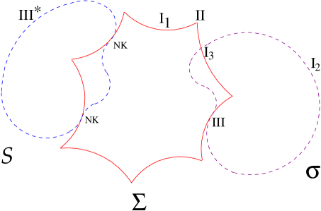
Figure 1: Schematic illustration of a discriminant curve. The fibers over the smooth parts of the curves ${\mathcal{S}}$, $\sigma$ and $\Sigma$ are of Kodaira type $III^{*}$, $I_{2}$ and $I_{1}$ respectively. The fibers over the cusp points of $\Sigma$ are of Kodaira type $II$. There are non-Kodaira fibers (NK) over the points where the ${\mathcal{S}}$ component intersects the $\Sigma$ components normally. There are $I_{3}$ fibers where the $\sigma$ component meets the $\Sigma$ component normally, and fibers of type $III$ where the $\sigma$ component intersects the $\Sigma$ component tangentially.

It was shown in a series of papers [1, 2, 3, 4, 5, 6, 7] that, when Hořava–Witten theory [8] is compactified on an elliptically fibered Calabi–Yau threefold, the requirements that there be three generations of quarks and leptons on the “observable brane” and that the theory be anomaly free generically necessitates the existence of wrapped M five–branes in the five–dimensional “bulk space”. These five–branes have two space–like dimensions wrapped on a holomorphic curve in the Calabi–Yau threefold. In [9] and in this paper, we are be interested in the case when this holomorphic curve is a pure fiber, ${\mathcal{C}}_{2}$. The five–brane worldvolume manifold is then $M_{4}\times{\mathcal{C}}_{2}$. The four dimensional theory arising from the wrapped five–brane has $N=1$ supersymmetry. However the amount of supersymmetry may be enhanced at low energies, depending on the five–brane location in the base. For ${\mathcal{C}}_{2}$ located at a generic point in the base, it can be shown that, at low energy, the $M_{4}$ worldvolume theory always contains a single $U(1)$ $N=4$ Abelian vector supermultiplet. However, if the fiber approaches any point on a smooth component of the discriminant curve, the $M_{4}$ worldvolume supersymmetry is enhanced to $N=2$. In addition to the $N=2$ decomposition of the $N=4$ supermultiplet, new light BPS hypermultiplets carrying $U(1)$ charges appear. The states may carry mutually non-local dyonic charges, which can not simultaneously be made purely electric by an $SL(2,Z)$ transformation. In that case, these theories are exotic and do not have a local Lagrangian description. When the five–brane wraps the degenerate fiber over the smooth component of the discriminant curve, the theory flows to an $N=2$ interacting fixed point in the infrared, of a type originally described (in a different context) in [32, 33, 34]. In [9], we considered only the smooth regions of the discriminant locus and using the theory of string junction lattices [27, 28] we presented strong constraints on the spectrum and the local and global charges of the additional light BPS hypermultiplets on $M_{4}$.

The discussion in [9] was restricted to smooth regions of the discriminant locus for two reasons. First, the supersymmetry at such points is $N=2$, and there are powerful constraints on the possible BPS multiplets [28]. Furthermore, the degenerate fibers over a smooth component of the discriminant curve fall entirely under Kodaira’s classification, and there is no ambiguity in the computation of the BPS states. However, neither of these is always a property of singularities of the discriminant locus, as we will see below.

The supersymmetry on a five–brane wrapped near such points is not always enhanced beyond $N=1$ at low energies. In these cases, a theory of a five brane wrapping a degenerate fiber over the singular point is an $N=1$ fixed point theory of the type discovered in [10]. In [10] these theories appeared in the context of three-brane probes of F-theory compactifications on elliptic Calabi-Yau threefolds. In [10], singularities of the discriminant locus giving rise to such singularities were identified, and certain anomalous dimensions were obtained. Like its $N=2$ counterpart, the low energy theory on a five-brane wrapped near a singularity of the discriminant curve is expected to have matter with mutually non-local charges, however much less is known about the spectrum. In this paper we begin a study of the spectrum near singularities of the discriminant curve.

In [9] we deformed the Weierstrass model so that the new discriminant curve was a local, disjoint union of $I_{1}$ curves. We showed that this method can be successfully applied to points on the smooth parts of the discriminant curve. In this paper, we extend these results to elliptic fibrations in a neighborhood of a singular locus of the fibration.

One could attempt to deform the Weierstrass model around a singular point $P_{0}$ of the discriminant in such a way that the new discriminant curve is a locally smooth curve with $I_{1}$ fibers. Deformations of this type could, in principle, be applied to some singular discriminant loci, albeit in a manner that differs significantly from the smooth case. Even in these cases, however, technical difficulties arise. We are motivated, therefore, to present some other procedure to “regulate” the singular loci. In other cases it is simply not possible to deform the isolated singularity of the discriminant.

Our approach will be the following: first, we will choose certain deformations of the Weierstrass model, so that the discriminant locus will still have the same multiplicity at $P_{0}$, and the nearby singular fibers are of Kodaira type $I_{1}$. We then “regulate” the singular point $P_{0}$ of the discriminant by surrounding it with an infinitesimal real sphere, $S^{3}$. A similar approach appeared in [32], in the context of $SU(3)$ ${N}=2$ Yang-Mills theory. The intersection of the discriminant curve with this sphere produces either a knot or a link in $S^{3}$ which is characteristic of the type of the singularity at $P_{0}$. All the points on this knot or link are within a smooth component of the discriminant curve of Kodaira type $I_{1}$. Any knot or link can be represented, but not uniquely, by a braid and an associated element of the braid group.

Next, we choose a braid and we seek the equivalence classes of string junctions on $S^{3}$, that is, the classes of junctions related by deformations and by Hanany-Witten transitions. Now, using the braid group and Hanany–Witten transformations, one can show that all possible $S^{3}$ string junction configurations are equivalent to a string junction in a real surface ${\cal{P}}$ transverse to the braid. This is possible because the allowed deformations do not change the singularity type of the general surface through $P_{0}$.

Since intersection number can be defined for membranes in the elliptic fibration over this surface, it follows that one can define the associated string junction lattice exactly as in [9, 27]. However, there remains an ambiguity that must be resolved. This arises from the fact that the braids associated with a given knot or link are not unique. We resolve these ambiguities by showing, using the braid group and Hanany–Witten transformations, that the string junction lattices associated with any two braid representations arising in this way are equivalent. In fact, we will show that the choice of an elliptic surface in the neighborhood of the singularity is related to the choice of a braid representative. The “general elliptic” surface corresponds to the “minimal braid” (defined in A.2); when our method can be applied, the junction lattice of the threefold is that of the general elliptic surface through $P_{0}$.

Our method cannot always be successfully applied. In Section 6 we give one such example: the supersymmetry here is broken to ${N}=1$ at the point $P_{0}$. In Section 7 we discuss the relationship with supersymmetry breaking.

The outline of the paper is as follows: in Section 2 we state the procedure; in Section 3 we recall basics facts about elliptic fibrations, singular fibers and discriminants. In Section 4 we consider an example where the discriminant has a singularity at a point $P_{0}$ and the nearby singular fibers are of Kodaira type $I_{1}$. In this case we do not need to deform the Weierstrass equation; instead we explain in details how two different braids give the same equivalence class of string junction lattices. In the Appendix, we explicitly describe the knot associated with this discriminant singularity and the two different braids in consideration.

In Section 5, we work out three examples where the discriminant has to be deformed. These examples illustrate the various rules stated in Section 2. It is worth noting that we can also recover the results of the previous paper [9], albeit by a less direct procedure. To illustrate this, in the first example of 5 we apply our procedure in a neighborhood of a point in the smooth part of the discriminant with Kodaira type $I_{2}$.

Remark: The order of vanishing of the discriminant of the threefold at $P_{0}$ coincides with the multiplicity of the discriminant of the general elliptic surface through $P_{0}$. The latter is the number of end points in the surface string junction lattice, which equals the number of strands in the minimal braid (see A.1 and A.2). This made us suspect that the multiplicity of an isolated curve singularity would always coincide with the number of strands of the minimal braid (also called the “index” of the knot, or link). It turns out that this statement is indeed always true; its proof is a hard and beautiful result. The first proof was given in [40]. A shorter, elegant proof is given by [41], using techniques from dynamical systems (see also [42] in the same volume, for an algebraic version). For an outline of the proof in the case of“ torus knots” (see the Appendix and, for example [44]).

2 Outline of our procedure

First, we will choose a deformation of the Weierstrass model around $P_{0}$, which fixes the order of vanishing of the discriminant at the origin, so that the other nearby singular fibers become of Kodaira type $I_{1}$. This imply that the general elliptic surface through the $P_{0}$ of the deformed model has the same type of singularity over $P_{0}$ as in the non-deformed model.

We then “regulate” the singular point $P_{0}$ of the discriminant by surrounding it with an infinitesimal real sphere, $S^{3}$. The intersection of the discriminant curve with this sphere produces either a knot or a link in $S^{3}$ which is characteristic of the type of the singularity at $P_{0}$ (see the Appendix). All the points on this knot or link are within a smooth component of the discriminant curve of Kodaira type $I_{1}$.

Next, we choose a braid representative of this knot (link) (see Appendix A) and we seek the equivalence classes of string junctions on $S^{3}$, that is, the classes of junctions related by deformations and by Hanany-Witten transformations. Note that there is nothing which forces junctions to live on this $S^{3}$. Actually they live in a four ball $B^{4}$ surrounding the singular point. However, we will assume that the equivalence classes of string junctions on $B^{4}$ are the same as the equivalence classes on $B^{4}-P_{0}$, where $P_{0}$ is the singular point. The endpoints of the junctions can then be slid along the discriminant curve, so that they lie entirely on the $S^{3}$ boundary of $B^{4}$. Now, using the braid group and Hanany–Witten transformations, one can show that all possible $S^{3}$ string junction configurations are equivalent to a string junction in a real surface ${\cal{P}}$ transverse to the braid. This is possible because the allowed deformations do not change the singularity type of the general surface through $P_{0}$.

Since intersection numbers can be defined for membranes in the elliptic fibration over this surface, it follows that one can define the associated string junction lattice exactly as in [9, 27]. However, there remains an ambiguity that must be resolved. This arises from the fact that the braids associated with a given knot or link are not unique. We resolve these ambiguities by showing, using the braid group and Hanany–Witten transformations, that the string junction lattices associated with any two braid representations arising in this way are equivalent. Furthermore we show that the string junction lattice in the threefold is the string junction lattice of “the minimal braid” associated to the knot(link) (see A.2 for the definition). The braid is obtained by “cutting” the discriminant with a (complex) curve $C_{R}$, which depends on the radius $R$ of the $S^{3}$; in the limit as $R\to 0$, $C_{R}$ becomes a general curve $C$ through $P_{0}$ (see A.3).

In our examples, the string junction lattice of the elliptic surface over $C$ coincides with the string junction lattice of the threefold. We speculate that this will not happen in more general cases, where the supersymmetry at $P_{0}$ is broken at ${N}=1$.

Note that with other deformations of the equation which do not satisfy our requirements, it is no longer clear how to understand a “cut” of this braid as a deformation of the original Kodaira type. This is because the requirement implies that the index (i.e. the minimal number of strands of an associated braid) of the knot (link) will stay the same before and after the “allowed deformations”. This can be explained as follow: On an elliptic surface, the string junction lattice is obtained by locally deforming the Weierstrass equation so as to split Kodaira fibers into fibers of $I_{1}$ type. The number of $I_{1}$ fibers into which a Kodaira fiber splits is determined by the order of vanishing of the discriminant. There are deformations which introduce more $I_{1}$ fibers entering from infinity, but none which increase the number locally. (In cases in which the Kodaira fiber corresponds to a conformal field theory, the deformations which introduce new $I_{1}$ fibers at infinity correspond to irrelevant deformations.) There is thus no smooth deformation which increases the number of states.

On an elliptically fibered Calabi-Yau, the string junction lattice may again be defined by splitting the fibers in the neighborhood of a singularity of the discriminant curve into $I_{1}$ type. The dimension of the string junction lattice is then obtained from the braid index of the resulting knot or link. As for a K3, we shall assume that there is no smooth deformation which increases the number of states by raising the dimension of the string junction lattice, (although in this case there may be deformations which lower the dimension.)

3 Basic facts about elliptic fibrations

A simple representation of an elliptic curve is given in the projective space ${\mathbb{C}}{\mathbb{P}}^{2}$ by the Weierstrass equation

$$zy^{2}=4x^{3}-g_{2}xz^{2}-g_{3}z^{3}$$ (3.1)

where $(x,y,z)$ are the homogeneous coordinates of ${\mathbb{C}}{\mathbb{P}}^{2}$ and $g_{2}$, $g_{3}$ are constants. The origin of the elliptic curve is located at $(x,y,z)=(0,1,0)$. The torus described by (3.1) can become degenerate if one of its cycles shrinks to zero. Such singular behavior is characterized by the vanishing of the discriminant

$$\Delta=g_{2}^{3}-27g_{3}^{2}$$ (3.2)

Equation (3.1) can also represent an elliptically fibered surface (or threefold), $W$, if the coefficients $g_{2}$ and $g_{3}$ in the Weierstrass equation are functions over a base curve (or surface) $B$ (see for example [9], for more details).

The resolved singular fibers of a Weierstrass model representing an elliptic curve are determined by the order of vanishing of $g_{2},g_{3}$ and $\Delta$; these fibers were classified by Kodaira:

Kodaira type	A-D-E	monodromy	N,L,K
$I_{n}$	$A_{n-1}$	$\begin{pmatrix}1&n\\ 0&1\end{pmatrix}$	$N=n,L=0,K=0$
$II$		$\begin{pmatrix}1&1\\ -1&0\end{pmatrix}$	${N=2,L>0,K=1}$
$III$	$A_{1}$	$\begin{pmatrix}0&1\\ -1&0\end{pmatrix}$	$N=3,L=1,K>1$
$IV$	$A_{2}$	$\begin{pmatrix}0&1\\ -1&-1\end{pmatrix}$	$N=4,L>1,K=2$
$I_{0}^{*}$	$D_{4}$	$\begin{pmatrix}-1&0\\ 0&-1\end{pmatrix}$	$N=6,L>1,K>2$
$I_{n}^{*}$	$D_{n+4}$	$\begin{pmatrix}-1&-n\\ 0&-1\end{pmatrix}$	$N=6+n,L=2,K=3$
$IV^{*}$	$E_{6}$	$\begin{pmatrix}-1&-1\\ 1&0\end{pmatrix}$	$N=8,L>2,K=4$
$III^{*}$	$E_{7}$	$\begin{pmatrix}-0&-1\\ 1&0\end{pmatrix}$	$N=9,L=3,K>4$
$II^{*}$	$E_{8}$	$\begin{pmatrix}0&-1\\ 1&1\end{pmatrix}$	$N=10,L>3,K=4$

Table 1: The integers $N$, $L$ and $K$ characterize the behavior of $\Delta$, $g_{2}$ and $g_{3}$ near the discriminant locus $u=0$; $\Delta=u^{N}a,g_{2}=u^{L}b$ , and $g_{3}=u^{K}c$ .

4 Regularizing without deforming the equation: a general cusp singularity of the discriminant

Isolated cusp points are a generic feature of discriminant curves. For example, in the discriminant locus shown in Figure $1$, there are $137$ cusps in the $\Sigma$ component of the curve. Note that any deformation of the Weierstrass equation corresponds to a change of coordinates in the $(s,t)$ plane. Thus it is never possible to remove the singularity of the discriminant by any deformation.

Consider one such cusp and choose local coordinates $s,t$ which vanish at that point. Then, in the neighborhood of the cusp, the sections $g_{2}$ and $g_{3}$, which define the elliptic fibration, can be taken to be

$$g_{2}=s,\qquad g_{3}=t$$ (4.1)

It follows that the Weierstrass representation of the fiber and the discriminant are given by

$$y^{2}=4x^{3}-sx-t$$ (4.2)

and

$$\Delta=s^{3}-27t^{2}$$ (4.3)

respectively.

Note that the Weierstrass model $y^{2}=x^{3}-t$ over the surface $s=0$ appears to be that of a type II Kodaira fiber at $t=0$, but the Weierstrass model $y^{2}=x^{3}-sx$ over the surface $t=0$ appears to be that of a type $III$ Kodaira fiber at $s=0$. To discuss the monodromy around a point in the discriminant locus of an elliptically fibered threefold, we could restrict to the fibration over a curve that intersects the discriminant locus at the cusp. The surface over generic curves, however, are smooth everywhere: note that the path ${\mathcal{P}}$ defined by $s=0$, which has coordinate $t$, is generic. For specificity, we take the intersecting surface to be the elliptic fibration over ${\mathcal{P}}$, which we denote by ${\cal{T}}$. Restricted to this surface, the cusp appears as a point in the one–dimensional complex base ${\mathcal{P}}$. Furthermore, restricted to ${\cal{T}}$, the discriminant and the Weierstrass representation are given by

$$\Delta=-27t^{2},\qquad y^{2}=4x^{3}-t$$ (4.4)

Both of these quantities are recognized as corresponding to a Kodaira type $II$ degeneration of the fiber at the cusp. Since the problem has now been reduced to an elliptic surface over a one–dimensional base, we can apply standard Kodaira theory to analyze the monodromy.

The $SL(2,{\mathbb{Z}})$ monodromy transformation for a Kodaira type $II$ fiber is given by

$${\cal{M}}_{II}=\begin{pmatrix}\ 1&1\\ -1&0\end{pmatrix}.$$ (4.5)

This transformation acts on the elements of $H_{1}({\mathcal{C}}_{2},{\mathbb{Z}})$, where ${\mathcal{C}}_{2}$ is the elliptic fiber. Note that ${\cal{M}}_{II}$ has no real eigenvector and, therefore, no obvious associated vanishing cycle. The usual way to proceed is to use the fact that ${\cal{M}}_{II}$ can be decomposed as

$${\cal{M}}_{II}=\begin{pmatrix}1&1\\ 0&1\end{pmatrix}\cdot\begin{pmatrix}2&1\\ -1&0\end{pmatrix}=A\cdot B$$ (4.6)

where both matrices $A,B$ are monodromies of Kodaira type $I_{1}$.

However, we have to justify the choice of the “generic” elliptic surface through $P_{0}$. It is in fact easy to see that non-generic surfaces will give different string junctions.

In order to resolve this ambiguity, following [32], we will consider, not the cusp itself, but the intersection of the discriminant curve

$$s^{3}-27t^{2}=0$$ (4.7)

with a l sphere $S^{3}$ of infinitesimal radius $R$ centered at the cusp. We will see in A.3 that the intersection is the “trefoil” knot shown in Figure $2$. All points in the knot lie in the smooth part of the discriminant curve, over which the elliptic fiber is of Kodaira type $I_{1}$, as shown in Figures $1$ and $2$.

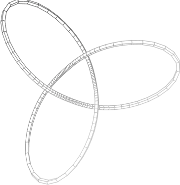
Figure 2: The trefoil knot associated with a cusp singularity. There is a Kodaira type $I_{1}$ fiber over every point in the knot.

To proceed, it is useful to represent the trefoil knot as a braid. This representation is not unique, as we will see in the Appendix. Two relevant braid representatives of the trefoil knot are shown in Figure $3$; we derive them explicitly in A.3.

Figure 3: Two equivalent braid representations of the trefoil knot (see also figure 16). The opposing endpoints are identified.

Note that any braid representative is a curve in ${{\mathbf{R}}}^{3}$. First, consider the two strand braid shown in Figure $3(a)$. This is obtained by cutting the knot with the line $s=c_{R}$, where $c_{R}$ is a constant depending on $R$ and $c_{R}\to 0$, as $R\to 0$ (see A.3). In this limit, this is one of the generic lines through the origin, intersecting the cusp with multiplicity $2$. Fix some arbitrary point $P$ in ${\mathbb{R}}^{3}$ (corresponding to the location of the wrapped M5-brane) which is not on the braid, and specify an ${\mathbb{R}}^{2}$ plane, ${\mathcal{P}}$, which contains $P$ and intersects the braid. This is shown in Figure $4(a)$. Note that the braid intersects ${\mathcal{P}}$ in two points. The elliptic fibration over ${\mathcal{P}}$, which we denote by ${\cal{T}}_{R}$, is our regularization of the surface ${\cal{T}}$. ${\cal{T}}_{R}$ has two separated discriminant points, each of Kodaira type $I_{1}$. In an appropriate basis, the monodromies around these two points in the plane ${\mathcal{P}}$ are $A$ and $B$ as defined in equation (2.6), as illustrated in figure $4(a)$. Note that in the planes over neighboring sections of the braid, the monodromies are different. The relation between monodromies in different sections of a braid is shown in Figure $5$. Next, extend a single string from $P$ to an arbitrary point on the braid which is not, in general, in ${\mathcal{P}}$. This point can always be moved back into the plane using a generalized Hanany–Witten mechanism. The result is a two–legged string junction that can be made to lie entirely in the ${\mathcal{P}}$ plane. This is shown in Figure $4$.

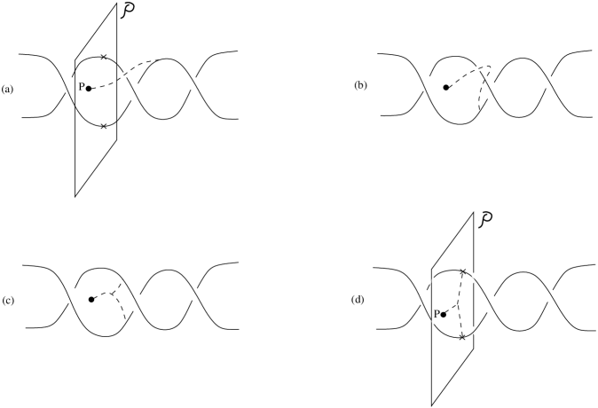
Figure 4: Mapping string junctions into a plane. By sliding the endpoints of the junction and doing Hanany–Witten transformations, as between Figures (b) and (c), any string junction can be brought into the plane, as in Figure (d).

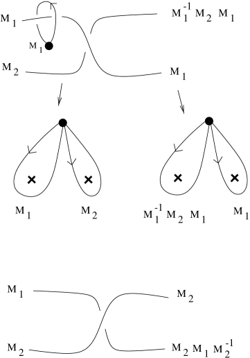
Figure 5: Illustration of the relation between $SL(2,Z)$ monodromies in different sections of a braid.

It is not hard to show that any string junction starting at $P$ can always be represented by a two–legged string junction in the plane ${\mathcal{P}}$. Note that the string junction lattice we obtain in this manner corresponds to a Kodaira type $II$ fiber degeneracy. Having put a junction in the plane, one can then slide endpoints of the junction lattice all the way around the braid and then do Hanany-Witten transitions to bring the junction back into the plane. This could, in principle, generate an additional equivalence relation, equating apparently different junctions in the plane ${\mathcal{P}}$. It is easy to see that, in this case, there is no such equivalence relation. This is because the total $(p,q)$ charge of a junction (or the boundary cycle of the membrane which results from lifting to M-theory) is not changed by this process. Since there are only two $I_{1}$ loci in the plane, the $p$ and $q$ charges completely determine the equivalence class of a junction in the plane (defined up to deformations and Hanany-Witten transitions within the plane). Thus, in this instance, the equivalence classes of junctions are the same as the equivalence classes of junctions restricted to the plane ${\mathcal{P}}$.

Before discussing these states, however, we would like to point out that one could have considered the surface over the line $t=0$. This line intersects the discriminant curve with multiplicity $3$. The path ${\mathcal{P}}$, with coordinate $s$, is here defined by $t=0$. To begin, denote the elliptic fibration over ${\mathcal{P}}$ by ${\cal{T}}$ and note that the cusp appears as a point in the one–dimensional complex base. Furthermore, the discriminant and Weierstrass representation are given by

$$\Delta=s^{3},\qquad y^{2}=4x^{3}-sx$$ (4.8)

which is the Weierstrass representation of a type $III$ Kodaira fiber in an elliptic surface. Since the problem has now been reduced to an elliptic two-fold, we can apply standard Kodaira theory to analyze the monodromy.

The $SL(2,{\mathbb{Z}})$ monodromy transformation for a Kodaira type $III$ fiber is given by

$${\cal{M}}_{III}=\begin{pmatrix}\ 0&1\\ -1&0\end{pmatrix}=A\cdot\ A\cdot B$$ (4.9)

where matrices $A,B$, defined in (4.6), both correspond to monodromies of Kodaira type $I_{1}$. Since ${\cal{M}}_{III}$ has no real eigenvector, one can attempt to proceed by deforming the discriminant curve from a single point of Kodaira type $III$ to three separate points, each of Kodaira type $I_{1}$. This deformation corresponds to the Weierstrass model of equation

$$y^{2}=4x^{3}-sx+t.$$

Here $t$ is the deformation parameter; the three $I_{1}$ fibers are found by considering the plane $t=c_{R}$, where $c_{R}$ is a constant (which depends on the radius $R$). These three singular fibers are exactly the ones obtained by a “vertical cut” (with the line $t=c_{R}$) in the 3-braided representation of the trefoil knot, as shown in Figure 3(b) (compare also with A.3).

Choose some point $P$ (corresponding to the location of the wrapped M 5-brane) which is not on the braid and specify a plane ${\mathcal{P}}$ which passes through $P$ and intersects the braid. This is depicted in Figure $6$. Note that the braid intersects ${\mathcal{P}}$ in three points. The elliptic fibration over ${\mathcal{P}}$, which we denote by ${\cal{T}}_{R}$, is our regularization of the surface ${\cal{T}}$. ${\cal{T}}_{R}$ has three separated discriminant points, each with Kodaira type $I_{1}$. The monodromies of each of these points can be computed and in an appropriate basis are the matrices $A$, $A$, and $B$ respectively in the plane ${\mathcal{P}}$ indicated in Figure 6.

By sliding string endpoints along the braid and using the Hanany–Witten mechanism, it can be shown that any string junction starting on $P$ and ending at arbitrary points on this braid can always be deformed to a three-legged string junction lying entirely within the plane ${\mathcal{P}}$.

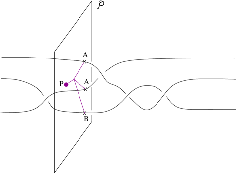
Figure 6: String junctions can always be brought into the plane intersecting the three–segment braid representation of the trefoil knot.

Note that the string junction lattice we obtain from this three–strand braid representation appears to be one associated with a Kodaira type $III$ fiber degeneracy and, hence, in contradiction with the above result. However, despite appearances, the string junction lattice associated with the three–strand braid is equivalent to the two–strand braid string junction lattice. Generically, the reason for this is the following. Unlike the type $III$ string junction lattices at a smooth point in the discriminant curve [9, 27], we can define a set of transformations where either one, two or all three legs of the junction can be translated along the braid until they return to the plane ${\mathcal{P}}$. As a rule, one will obtain a different string junction in the plane ${\mathcal{P}}$. However, by construction, this new junction must be equivalent to the original one. That is, not all Kodaira type $III$ string junctions near a cusp are independent. We now proceed to show that, in fact, only a Kodaira type $II$ subset of string junctions are independent.

The braid under consideration is divided into sections, each with three parallel lines. An element of the braid group acts between each section by intertwining the three lines. As one moves the junction from one section to the next, one can do a Hanany-Witten transition to keep it in a canonical form within a plane intersecting the braid section, in which the junction lies in the upper half-plane. In this way, the braid group acts on string junctions restricted to the plane. As one goes all the way around the braid, string junctions $J$ in the plane ${\mathcal{P}}$ are acted on by the (three-strand) braid group element of the knot ${\mathcal{G}}$, giving another string junction $J^{\prime}$ which is equivalent to $J$

$${\mathcal{G}}J=J^{\prime}\sim J$$ (4.10)

Such an equivalence would not exist if we were considering the junction lattice of a type $III$ fiber in an elliptic two-fold instead of a three-fold. The string junction lattice is thus the quotient of the string junction lattice restricted to the plane ${\mathcal{P}}$ by the action of the braid group. To see explicitly how the quotient acts, consider an oriented string, denoted by $\vec{\alpha}$, connecting the two discriminant points in the ${\mathcal{P}}$ plane in Figure $6$ with identical monodromy matrix $A$. Translating this string along the braid, we find that it returns to the plane ${\mathcal{P}}$ with its orientation reversed, as illustrated in Figure $7$. We have indicated in the figure the canonical form of the junction which arises as one moves around the braid. Within each section of the braid, the junction may be written as a vector $\vec{\alpha}=n_{1}{\vec{v}}_{1}+n_{2}{\vec{v}}_{2}+n_{3}{\vec{v}}_{3}$, where ${\vec{v}}_{i}$ is a single string with an endpoint on the i’th segment of the braid, labelled from top to bottom. As one moves around the braid, starting from the point indicated, $\vec{\alpha}$ is transformed as follows

$${\vec{\alpha}}={\vec{v}}_{1}-{\vec{v}}_{3}\rightarrow{\vec{v}}_{1}+{\vec{v}}_{3}-{\vec{v}}_{2}\rightarrow{\vec{v}}_{3}-{\vec{v}}_{1}\rightarrow{\vec{v}}_{2}+{\vec{v}}_{3}-{\vec{v}}_{1}\rightarrow{\vec{v}}_{3}-{\vec{v}}_{1}=-{\vec{\alpha}}$$ (4.11)

This sequence is illustrated in Figure $7$. It follows that $\vec{\alpha}$ is equivalent to zero. Therefore,as illustrated in Figure 8, given any junction we can, by Hanany-Witten transformations, write it as a two strand junction in the plane ${\mathcal{P}}$ with an endpoint on the strand with monodromy $B$ and an endpoint on one of the strands with monodromy $A$. There can be no further equivalence relation because the dimension of the lattice must be at least two to get all possible $(p,q)$ boundary cycles. Thus one has the same two dimensional string junction lattice that one obtains for a type $II$ Kodaira fiber.

Another way of stating the above result is the following. Given the Weierstrass model $y^{2}=4x^{3}-sx-t$, one can find the lattice of string junctions restricted to a curve of constant non-zero $t$. One then quotients by the monodromy which acts on this lattice as one moves this curve in a circle around $t=0$ . This gives the same result as restricting to curve of constant non-zero $s$, and quotienting by the (in this case trivial) monodromy which acts when one moves the curve in a circle around $s=0$.

In this Section, we have only proven the equivalence of the two and three-braid string junction lattices. However, using these techniques it is not hard to demonstrate this equivalence for all braid representations of the trefoil knot. It follows that the correct structure of the string junction lattice at a cusp, Kodaira type $II$, is most easily obtained from the two-braid representation. As discussed above, this corresponds to choosing the curve intersecting the cusp to be generic. In general, it turns out that the junction lattice in the neighborhood of a singularity of the discriminant curve is determined by the $SL(2,Z)$ monodromy around the singular point within a generic slice. In the present example, a generic slice containing the cusp is given locally by $s+\lambda t=0$ for finite $\lambda$. The restriction of the Weierstrass equation to this slice is $y^{2}=4x^{3}+\lambda tx-t$, with the discriminant $\Delta=t^{2}(-\lambda^{3}t-27)$. The monodromy around $t=0$ is that of a type $II$ Kodaira fiber. This completely resolves the discrepancy discussed above. That is, the junction lattice is that of a type $II$ Kodaira fiber on an elliptic surface. In fact, in this case, the fiber at the cusp happens to be a type $II$ Kodaira fiber. Later, we will encounter examples in which the fiber type does not match the junction lattice.

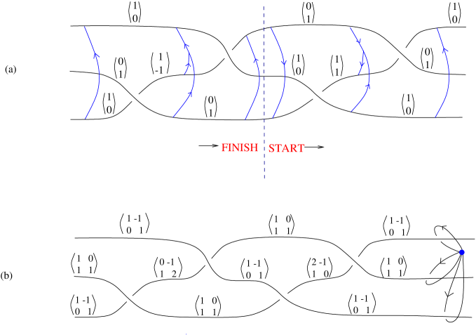
Figure 7: (a) The root junction $\vec{\alpha}$ can be transformed to $-\vec{\alpha}$ by a translation all the way around the braid. As one moves from one section of the braid to the next, Hanany-Witten transitions are performed to keep the junction in a canonical form in the upper half of a plane transverse to the braid. The vanishing cycles with respect to a path in the upper half plane are indicated above each segment of the braid. The vanishing cycles are eigenvectors of the monodromies indicated in (b).

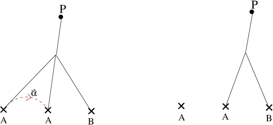
Figure 8: In the three–strand braid representation of the trefoil, the root junction $\vec{\alpha}$ is equivalent to zero. Therefore, any string junctions related by the addition or subtraction of $\vec{\alpha}$ are equivalent. Thus, the string junction lattice is actually that of a Kodaira type $II$, rather than of type $III$.

The string junction lattice is only part of what is required to determine the spectrum of light charged matter on a five–brane wrapped near a singularity. Extra constraints are required, which we will discuss later. In this particular example, however, we expect that the infrared limit of the five-brane worldvolume theory in the neighborhood of the cusp is the same as that in the neighborhood of a type $II$ Kodaira fiber over a smooth component of the discriminant curve. This is because, based on arguments in [10], the cusp singularity can not describe a conformal fixed point with a Weierstrass form invariant under scale transformations. Furthermore, the operators which deform a smooth type $II$ into a cusp are irrelevant, while those which deform a smooth type $III$ into a cusp are relevant. This is consistent with the result that the string junction lattice is that of a type $II$. We conclude that the light state spectrum at a cusp singularity is $N=2$ supersymmetric and identical to the spectrum for a Kodaira type $II$ fiber over points in the smooth part of the discriminant curve. This spectrum was computed in [9, 28].

5 Deforming the equation: normal crossing intersections of the discriminant

In the previous section, we gave an example of a singularity where it was not necessary to deform the discriminant curve, since the Kodaira type fibers in a neighborhood of $P_{0}$ are of type $I_{1}$. Here we present three different examples where the Kodaira type fibers in a neighborhood of $P_{0}$ are no longer of type $I_{1}$. Therefore, in these examples, we first need to deform the discriminant curve, before regularizing the singularity with the sphere $S^{3}$. In the case of the normal crossing intersection, the links on $S^{3}$ are, in fact, simple linked circles and there is an obvious minimal braid (with no extra relations on the string junction lattice). Thus, while in the previous example we focused on the braids, in the following examples we will focus on the deformations.

Before we consider the examples of simple normal crossing singularities, we will revisit the case of a smooth part of the discriminant curve, as discussed in [9]. Unlike [9], however, in this section we will use a deformation which leaves the multiplicity of the discriminant fixed at a point and regularize the singularity with the sphere $S^{3}$. All the examples in [9] could have been computed in this manner. We present this method here, since it gives a simple illustration of the features which will occur, in a more complicated form, for simple normal crossing singularities.

5.1 The smooth locus of the discriminant

We consider the smooth part of the discriminant of Kodaira type $I_{2}$, in Figure 1. Pick any point $P_{0}$ on the smooth part of $\sigma$, and choose the origin of the $s,t$ coordinates to be at that point. In the neighborhood of this point, the associated sections have the form

$$g_{2}=3a^{2},\qquad g_{3}=a^{3}-s^{2},\qquad\Delta=s^{2}f^{2}$$ (5.1)

where $a$ and $f$, to leading order in $s$, are non–zero functions of $t$ only. (See for example, Table $1$ in Section 3.

We choose a deformation of the Weierstrass representation which fixes the order of vanishing (here the order of vanishing is $2$) of the discriminant at the origin. After the deformation, the singular fibers outside the origin become of Kodaira type $I_{1}$. A suitable such deformation of the equation has the form

$$y^{2}=4x^{3}-3a^{2}x-(a^{3}-(s+\epsilon t)(s-\epsilon t))$$ (5.2)

with discriminant

$$\Delta_{\epsilon}=(s+\epsilon t)(s-\epsilon t)b,$$ (5.3)

where $b$ does not vanish near $P_{0}$. Note that this is also the “relevant” deformation used in [9] of the general elliptic surface through $P_{0}$, with $\epsilon t$ the deformation parameter.

The general elliptic surface of the deformed model through $P_{0}$ (obtained by setting, say $t=0$) also has Kodaira type fiber of type $I_{2}$. Similarly, the order of vanishing of the discriminant at $P_{0}$ is $2$, both in the deformed and non-deformed models. This satisfies the rules stated in Section 2. Then, as for the cusp singularity, we will regulate the crossing point by considering the intersection of the deformed discriminant curve with the sphere $S^{3}$ of infinitesimal radius $R$ centered $P_{0}$. We obtain the “link” shown in Figure 9 (see Appendix A and A.3). Since this link is composed of points all in the smooth part of the discriminant curve, the Kodaira type of fiber degeneration over any point in the link can be determined by canonical methods.

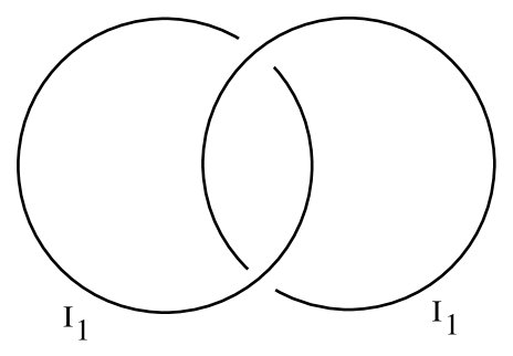
Figure 9: Link associated to the deformed $I_{2}$ smooth locus.

As before, we represent this link as a braid. Since this link is so simple, the proof that the string junction lattice is that of the minimal braid is straightforward. This minimal braid (see A.2) is shown in Figure $10$.

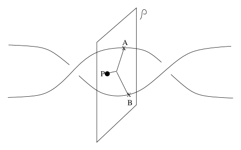
Figure 10: Minimal braid associated to the deformed $I_{2}$ smooth locus.

Note that the braid intersects ${\mathcal{P}}$ in two points. The elliptic fibration over ${\mathcal{P}}$, which we denote by ${\cal{T}}_{R}$, is our regularization of the surface ${\cal{T}}$. ${\cal{T}}_{R}$ has two separated discriminant points, with Kodaira type $I_{1}$. The monodromies of these points can be computed and are found to be of type $A$. Using the Hanany–Witten mechanism, it is not too hard to show that any string junction starting at $P$ can always be represented by a two–legged string junction in the plane ${\mathcal{P}}$. Note that the string junction we obtain in this manner corresponds to a two Kodaira type $I_{1}$ fiber degeneracy.

Because the braid is composed by two simply linked segments, there are no further relations on the string junction lattice in the plane $\cal P$, which is the lattice of a type $I_{2}$. Note that the vanishing of the discriminant at $P_{0}$ is equal to the number of strands of the braid. This is a general fact, see A.2 and the end of the Introduction. Without the restriction on the allowed deformations, we could have obtained a braid with fewer strands. It would no longer have been clear how to see a “cut” of this braid as a deformation of the Kodaira type $I^{2}$.

In general, if $P_{0}$ is a smooth point of the discriminant, then any allowed deformation is also a deformation of the general elliptic surface through $P_{0}$. The associated link is given by $n$ simple linked circles, where $n$ is the order of vanishing of the discriminant at $P_{0}$. The associated minimal braid has $n$ strands, because we have $n$ distinct links; any allowed deformation is also a deformation of the general elliptic surface through $P_{0}$. Hence, we find the string junction lattice of the general surface through $P_{0}$.

5.2 Simple Normal Crossing Intersection: Kodaira type $I_{1}$ and $I_{2}$

We now apply the techniques described in the previous subsection to simple normal crossing intersection of the discriminant curve. In the discriminant locus shown in Figure $1$, there are $28$ simple normal crossing intersections of the components $\Sigma$ and $\sigma$ of the curve. Consider one such intersection $P_{0}$ and choose local coordinates $s,t$ around $P_{0}$. Then, in the neighborhood of this point, the sections $g_{2}$ and $g_{3}$ can be taken to be

$$g_{2}=3a^{2},\qquad g_{3}=a^{3}-s^{2}t,$$ (5.4)

where $a$ is a suitable constant (see Section 3). The equations of the Weierstrass model and the discriminant are given by

$$y^{2}=4x^{3}-3a^{2}x-(a^{3}-s^{2}t)$$ (5.5)

and

$$\Delta_{\epsilon}=s^{2}t[-2a^{3}+s^{2}t]$$ (5.6)

respectively. We choose a deformation of the Weierstrass representation which fixes the order of vanishing of the discriminant at the origin, while the singular fibers outside the origin become Kodaira type $I_{1}$.

The equation of the deformed Weierstrass threefold and the discriminant are given by

$$y^{2}=4x^{3}-3a^{2}x-(a^{3}-(s+\epsilon t)(s-\epsilon t))t$$ (5.7)

and

$$\Delta=(s+\epsilon t)(s-\epsilon t)t[-2a^{3}+(s+\epsilon t)(s-\epsilon t)t]$$ (5.8)

respectively. We see that any point with Kodaira type $I_{2}$, is split into two nearby discriminant points, each of Kodaira type $I_{1}$. Note that the general elliptic surface of the deformed model through $P_{0}$ (obtained, by setting, say, $t=s$) has the same type of singularities as the non-deformed one and that the multiplicity of the discriminant through $P_{0}$ is unchanged in the deformed and non-deformed models. This satisfies the rules stated in Section 2. Then, as in the previous example, we will regulate the crossing point by considering the intersection of the deformed discriminant curve with the sphere $S^{3}$ of infinitesimal radius $R$ centered $P_{0}$. We now obtain the “link” shown in Figure $11$. Again, this link is composed of points all in the smooth part of the discriminant curve and the Kodaira type of fiber degeneration over any point in the knot can be determined by canonical methods.

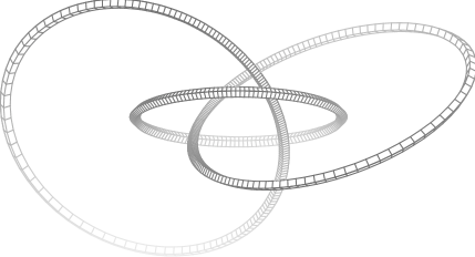
Figure 11: Link associated to the deformed $I_{2}$-$I_{1}$ intersection.

Next, we represent this link as a braid. Among the various braids representations we will consider only the simplest braid representation, which corresponds to choosing a generic base curve for the intersecting surface. This minimal braid (see A.2) is shown in Figure $12$.

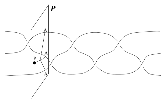
Figure 12: Minimal braid associated to the deformed $I_{2}$-$I_{1}$ intersection.

Note that the braid intersects ${\mathcal{P}}$ in three points. The elliptic fibration over ${\mathcal{P}}$, which we denote by ${\cal{T}}_{R}$, is our regularization of the surface ${\cal{T}}$. ${\cal{T}}_{R}$ has three separated discriminant points, with Kodaira type $I_{1}$. The monodromies of these points can be computed and are found to be of type $A$. This is indicated pictorially in Figure $12$. Using the Hanany–Witten mechanism, it is not too hard to show that any string junction starting at $P$ can always be represented by a three–legged string junction in the plane ${\mathcal{P}}$. As in the previous example, because the braid does not induce any relations among the end points, the associated string junction lattice has monodromy structure $A\cdot A\cdot A$. This is the lattice of a type $I_{3}$ fiber. Therefore, the light state spectrum at the $I_{1}-I_{2}$ simple normal crossing identifies to that of a type $I_{3}$ fiber over a smooth part of the discriminant. This spectrum was presented in [9].

5.3 Simple Normal Crossing Intersection: Kodaira type $I_{1}$ and $I^{*}_{0}$

Here we consider another type of simple normal crossing intersection, which also occurs in case 1 of example 2 in [9]. Two different components $\Sigma$ and ${\cal{S}}$ of the discriminant, of Kodaira type $I_{1}$ and $I^{*}_{0}$ respectively, meet with a simple normal crossing intersection at a point $P_{0}$. We can choose local coordinates $s,t$ around $P_{0}$, with $P_{0}$ as the origin. Then, in the neighborhood of this point, the sections $g_{2}$ and $g_{3}$ can be taken to be

$$g_{2}=3(sa)^{2},\qquad g_{3}=(ac)^{3}-s^{3}t,$$ (5.9)

where $a$ is a suitable function (see Section 3). The equation of the deformed Weierstrass threefold and the discriminant are given by

$$y^{2}=4x^{3}-3(sa)^{2}x+(sa)^{3}+t(s^{3})$$ (5.10)

$$t\cdot(s^{6})\cdot(4a^{3}+t)=0.$$ (5.11)

As before, we choose a deformation of the Weierstrass representation which fixes the singularity of the discriminant at the origin, so that the singular fibers outside the origin become of type $I_{1}$ in the deformed model. The equation of the deformed Weierstrass threefold and the discriminant are given by

$$y^{2}=4x^{3}-3(sa)^{2}x+(sa)^{3}+t(s^{3}-\epsilon^{3}t^{3})$$ (5.12)

$$t\cdot(s-\epsilon t)\cdot(s-\epsilon e^{\frac{2\pi i}{3}}t)\cdot(s-\epsilon e^{\frac{4\pi i}{3}}t)\cdot(-\epsilon^{3}t^{4}+s^{3}(4a^{3}+t))=0.$$ (5.13)

This Weierstrass model defines a threefold $W_{\epsilon}$, which is smooth outside the point $y=x=t=s=0$ ($a$ is non-zero at the origin). The singular fibers are of type $I_{1}$, except at the point ${s=t=0}$. This deformation preserves the type of singularity of the generic elliptic surface through $P$. The corresponding braid can be shown to be a $7$-braid. It is more complicated to draw, so we limit ourselves to describe it in words, and display the (MAPLE generated) picture of the corresponding knot. The braid is composed of four simple linked circles (as in the previous example) and a 3-stranded minimal braid. It is easy to see that, by cutting with a general real plane $\cal P$, we obtain a monodromy structure of type $A^{5}\cdot B\cdot C$. Since there are no further relations among the different strands, this will also be the monodromy structure in the threefold. From Table 4 in [9], we find that the corresponding junction lattice is that of a type $I^{*}_{1}$ singularity. Therefore, the light state spectrum at the $I_{1}-I^{*}_{0}$ simple normal crossing identifies to that of a type $I_{1}^{*}$ fiber over a smooth part of the discriminant.

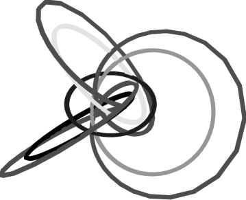
Figure 13: Knot corresponding to the deformed $I^{*}_{1}$ and $I^{*}_{0}$ simple normal crossing intersection.

6 A puzzle: Non-transversal Intersections

We also studied many examples of non-transversal intersections. We found that in these cases no deformation leaves the $I_{1}$ locus fixed, and that we cannot determine which strands of the knot correspond to the deformation of the un-deformed points of the discriminant. Therefore, the two-dimensional analysis cannot be used in these examples. This might indicate that supersymmetry is broken at the point $P_{0}$, and that the string junction lattice of the threefold no longer coincides with that of the general elliptic surface through $P_{0}$, as in the ${N}=2$ case. As an example of this problem, let us consider a case where the supersymmetry is known to be broken to ${N}=1$.

In the discriminant locus shown in Figure $1$, there are $5$ non-transversal intersections of the components $\Sigma$ and ${\mathcal{S}}$ of the curve. Let us consider one such intersection point and choose local coordinates $s,t$ which vanish at that point. Then, in the neighborhood of this point, the sections $g_{2}$ and $g_{3}$ can be taken to be

$$g_{2}=st^{3},\qquad g_{3}=t^{5}$$ (6.1)

It follows that the Weierstrass representation of the fiber and the discriminant are given by

$$y^{2}=4x^{3}-st^{3}x-t^{5}$$ (6.2)

and

$$\Delta=t^{9}(s^{3}-27t)$$ (6.3)

respectively. The Kodaira type over $t=0$ is of type $III^{*}$. A possible allowed deformation is

$$y^{2}=4x^{3}-st^{3}x-(t^{5}+\epsilon s^{5})$$ (6.4)

with discriminant

$$\Delta=t^{9}s^{3}-27(t^{10}+\epsilon^{2}s^{10}+2\epsilon t^{5}s^{5})$$ (6.5)

Because deformation does not leave the (original) $I_{1}$ locus fixed, we cannot determine which strands of the knot correspond to the deformation of the $III^{*}$ locus. We do not believe that any such deformation exists. This makes examples of this kind completely different from the $N=2$ cases discussed previously in this paper.

7 Supersymmetry at Low Energy.

The field theory on the worldvolume of a five-brane in the bulk has ${N}=1$ supersymmetry. However, the amount of supersymmetry may be greater in the infrared limit. For example, if the five-brane wraps an elliptic curve over a generic point in the base of the Calabi-Yau threefold away from the discriminant curve, the IR theory is an ${N}=4$ $U(1)$ gauge theory. This can be understood heuristically as a consequence of the correspondence between long distances on the five-brane and short distances in the transverse space-time. In the IR, the five-brane probes only the local transverse geometry of the Calabi-Yau base, which is ${\mathbf{R}}^{4}$ when the brane wraps a fiber over a generic point in the base. In the IR, the scalar fields associated with this ${\mathbf{R}}^{4}$, together with the axion and $S_{1}/Z_{2}$ moduli, belong to a multiplet under the ${N}=4$ $SO(6)$ R symmetry. The situation is different when the five-brane wraps a fiber over the discriminant curve. When this fiber lies over a smooth component of the discriminant curve, the IR theory has ${N}=2$ supersymmetry.

When the fiber lies over a singular point of the discriminant curve, infrared properties can be studied using the methods of [10]. The authors of [10], studied the low energy theories of three-brane probes of Calabi-Yau geometries in F-theory, which are the same as the theories which arise in our context. If the IR theory is an interacting fixed point with ${N}=1$ supersymmetry, then the local form of the singularity is preserved by IR flow, meaning that the local Weierstrass equation,

$$y^{2}=x^{3}-f(s,t)x-g(s,t).$$ (7.1)

is invariant under scaling when appropriate dimensions are assigned to $x,y,u$ and $v$. The holomorphic three-form of the Calabi-Yau threefold,

$$\Omega=\frac{ds\wedge dx\wedge dt}{2y}$$ (7.2)

should have dimension $[\Omega]=2$ (see [10]). Furthermore, for unitarity one requires $[s]>1$ and $dim[t]>1$.

As an example, consider the tangential crossing of $III^{*}$ with $I_{1}$ described by

$$y^{2}=4x^{3}-st^{3}x-t^{5},$$ (7.3)

with a five-brane wrapped over the point $s=t=0$. This example (discussed in [10]) is consistent with an ${N}=1$ CFT in the infrared limit. The scaling relations $2[y]=3[x]=[s]+3[t]+[x]=5[t]$ and $[\Omega]=[s]+[t]+[x]-[y]=2$ gives the anomalous dimensions $[s]=4/3$ and $[t]=4$.

When the conditions for ${N}=1$ supersymmetry in the IR are not satisfied, one expects the theory to flow to an ${N}=2$ fixed point in the infrared limit. Heuristically, one can understand this process as a smoothing of the singularity, such that the local geometry seen by the five-brane looks like that over a smooth component of the discriminant curve. As an example, consider the cusp singularity $y^{2}=4x^{3}-sx-t$, with a five-brane wrapped over the point $s=t=0$. In the infrared limit, the theory flows to a CFT with no dimensional parameters. If this CFT has $N=1$ supersymmetry, the discriminant curve singularity should be fixed under the infrared flow, that is the Weierstrass equation above should have no dimensional parameters. The dimensions would have to satisfy the following relations: $2[y]=3[x]=[s]+[x]=[t]$, and also that $[\Omega]=[s]+[t]+[x]-[y]=2$ . This would imply that $[s]=8/9$, which is not consistent with the unitarity bound $[s]\geq 1$ on scalar fields in a unitary superconformal theory. Thus the cusp can not describe a non-trivial $N=1$ fixed point. A natural guess is that the theory flows in the infrared to an $N=2$ conformal theory, described either by the Weierstrass model $y^{2}=4x^{3}-t$ or by $y^{2}=4x^{3}-sx$. The former possibility seems more likely for the following reasons. In the $N=2$ CFT described by $y^{2}=4x^{3}-t$, the scaling dimension of $[s]$ is $1$, as $s$ is a free scalar field describing motion parallel to the discriminant curve. The scaling relation $2[y]=3[x]=[t]$, together with $[\Omega]=[s]+[t]+[x]-[y]=2$ yields $[t]=6/5$. Then the (analytic) deformation which gives a cusp singularity is given by $y^{2}=4x^{3}-\epsilon sx-t$. This deformation is irrelevant since $[\epsilon]=-1/5$. However, for the $N=2$ CFT described by $y^{2}=4x^{3}-sx$, the scaling dimensions satisfy $[t]=1$, $2[y]=3[x]=[s]+[x]$ and $[\Omega]=[s]+[t]+[x]-[y]=2$. This means that the deformation which gives a cusp singularity, $y^{2}=4x^{3}-sx-\epsilon t$, is relevant since $[\epsilon]=1$. This suggests that in the infrared limit, the theory described by the cusp singularity flows to an $N=2$ CFT described by the Weierstrass model of a type $II$ Kodaira fiber over a smooth component of the discriminant curve.

As one further example, consider the simple normal crossing of $I_{2}$ with $I_{1}$ described by $y^{2}=4x^{3}-3a^{2}x-(a^{3}-s^{2}t)$, with a five-brane wrapped over $s=t=0$. There is no way to assign scaling dimensions, so that there are no dimensional parameters in the Weierstrass model. Hence $[s]$ and $[t]$ have dimension $>1$, and $[\Omega]=2$. One would have to satisfy $2[y]=3[x]=2[a]+[x]=3[a]=2[s]+[t]$, but if the parameter $a$ has dimension zero, then $2[s]+[t]=0$ and $[\Omega]=[s]+[t]=2$. Note that, in this example, the $I_{2}$ and $I_{1}$ fibers are mutually local (same vanishing cycle), so that there are no states with mutually non-local $(p,q)$ charges. Consequently one does not expect to find a non-trivial CFT in the infrared limit. The IR flow will never give a local form of the Weierstrass equation which is invariant under scaling. The low energy theory is a $U(1)$ gauge theory with electrically charged matter, and flows to a free theory in the infrared limit.

Acknowledgements We would like to thank B. Johnson, P. Melvin and L. Zulli for helpful conversations.

B. Ovrut is supported in part by the DOE under contract No. DE-ACO2-76-ER-03071. A. Grassi’s research was supported in part by NSF grants DMS-9706707 and DMS-0074980. Part of this work was completed while A.G. was a member at the Institute for Advanced Study, Princeton, NJ and supported by N.S.F. grant DMS-9729992. Z. Guralnik is supported in part by the DOE under contract No. DE-ACO2-76-ER-03071.

Appendix: Curve Singularities, Knots and Braids

In this section, we derive examples of knots (or links) and braids associated to an isolated plane curve singularity. In [37] Milnor studied properties of isolated (complex) singularities of hypersurfaces in ${\mathbf{C}}^{n}={\mathbf{R}}^{2n}$ by intersecting the hypersurface with a sphere $S^{2n-1}$ of radius $R$ centered at the singularity. In the case of complex plane curves, the intersection is a real curve, called a knot, if it has one component, a link otherwise. These are also called algebraic knots (links). The idea is that the type of singularity of the curve is closely related to the topological property of the associated knot (or link). For example, as we will see below, the knot associated with a smooth point is a circle (unknot).

Take $(s,t)$ to be complex coordinates in the plane ${\mathbf{C}}^{2}\sim{\mathbf{R}}^{4}$, so that the complex curve has an isolated singularity at the point ${(s,t)=(0,0)}$. To describe the intersection of the curve and $S^{3}$ it is easier to use polar coordinates:

$$\xi e^{i\theta}=t,\eta e^{i\phi}=s;$$

the equation of the sphere of radius $R$ is then $\xi^{2}+\eta^{2}=R^{2}$. Recall that $S^{3}$ can also be thought of two solid tori glued along the boundary. In the example we consider, the intersection of the complex curve with $S^{3}$ will be a knot (or link) on the (boundary of) tori. These are called torus knots (or links).

A.1: A smooth point is the unknot

Let us assume that ${s=0}$ is the local equation of the curve around the origin. It is easy to see that the intersection of the curve with the sphere $\xi^{2}+\eta^{2}=R^{2}$ is a circle $S^{1}$ of radius $R$. We can cut the circle in a point and obtain a line segment; we can recover the circle by identifying the endpoints of the segment. The segment is called an associated braid. Similarly, given a braid, we obtain a knot by closing the braid. For a precise definition of a braid see, for example, [38] and [44].

A.2: On braids

We can associate many different braids to a knot; it is a hard result that every knot (link) can be represented by a closed braid [39]; (see again [38] and [44]). Many different braids can be associated to a knot (link) [38] (2.14). Among the different braid representations of the knot, the one with the fewest strands is called the minimal braid. The number of strands of the minimal braid is called the braid index. The braid index is an invariant of the knot [38]. Our analysis of string junction lattices led us to conjecture that the braid index of these algebraic knot would always be equal to the order of vanishing of the complex curve at $(s,t)=(0,0)$. It turns out that this statement is indeed always true, but it is a hard and beautiful result. The first proof was given in [40]. A shorter, elegant proof is given by [41], using technique from dynamical system (see also [42] in the same volume, for an algebraic version). In the above example, for the smooth point (i.e. the order of vanishing is one), we have a one strand braid.

A.3: An isolated cusp singularity and the trefoil knot

As in Section 4, we take $t^{2}+s^{3}=0$ to be the local equation of the singularity. (Note that the order of vanishing is two, and we will find a two-strand minimal braid). We show that we obtain the trefoil knot, and we construct two braids, the minimal two-strand braid and a three-stranded braid. It is easy to see that the intersection of the discriminant and the sphere $S^{3}_{R}$ of radius $R$ centered at the origin is the parametric curve:

$$(t,s)=(\xi_{0}e^{i3\theta},\eta_{0}e^{i\frac{\pi}{3}}e^{i2\theta}),$$

where $\xi_{0}$ and $\eta_{0}$ are fixed positive constant which depend on $R$. From the parametric equation we see that this real curve lies on $S^{1}\times S^{1}$, the product of two circles of radius $\xi_{0}$ and $\eta_{0}$ respectively; the exponential $(e^{i3\theta},e^{i2\theta})$ give a slope of $(3,2)$ on the square obtained by “cutting open” the torus (see Figure 14).

Figure 14: The torus is obtained by identifying the top with the bottom and the left with the right side. The horizontal line is the $t$ axis ($s=0$), while the vertical one is the $s$ axis ($t=0$). The slanted line represents the intersection of the complex curve of equation $t^{2}+s^{3}=0$ and $S^{3}$ of slope $(3,2)$. Note that a vertical cut corresponds on the plane $(s,t)$ with the line $s$ constant, and an horizontal cut with the line $t$ constant.

This curve is connected, hence it is a knot; it is often denoted as the $(3,2)$ torus knot. In Figure 15 we can see that this knot is exactly the trefoil knot of Figure 2 in Section 4.

A general result shows that all the knots obtained by intersecting a complex curve with $S^{3}$ are torus knots or can be described from torus knots (the “iterated torus knots”).

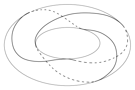
Figure 15: The $(3,2)$ knot is the trefoil.

In the next Figure 16 we show that by “folding” the square in Figure 14 horizontally (vertically), we obtain a two (three)-strand braid. These foldings correspond to cutting the torus (and the knot) along a horizontal (resp vertical) meridian.

Figure 16: Two braids representations of the $(3,2)$ torus knot. The two braids are obtained by cutting the torus along the meridian and the longitude. This corresponds by folding the square in the previous pictures in half, first horizontally then vertically.

It is easy to see that the first braid corresponds to a cut $t=c_{1}$ and the second to a cut $s=c_{2}$, where $c_{1}$ and $c_{2}$ are constants depending on $R$, the radius of $S^{3}$. In the limit $R\to 0$, the first $s=c_{1}$ cut intersects the cuspidal curve with multiplicity $2$ (a generic intersection), while the second cut $s=c_{2}$ has intersection multiplicity $3$.

A.4: A transversal intersection (nodal singularity)

Here we consider a local equation $(s+\epsilon t)(s-\epsilon t)=0$, as in Section 5.1; instead of a knot, we will obtain a link. It is easy to see the intersection of the curve with $S^{3}$ lives again on $S^{1}\times S^{1}$. In the following Figure 17 we represent this torus by a square with identified sides, and the braid obtained by folding horizontally (as in the previous section). We see that we have two differen simply linked components.

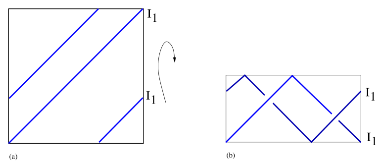
Figure 17: The link associated with a nodal singularity and a two-strand braid.

References

- [1] A. Lukas, B. A. Ovrut, K. S. Stelle and D. Waldram, The Universe as a Domain Wall, Phys.Rev. D59 (1999) 086001; Heterotic M-theory in Five Dimensions, Nucl.Phys. B552 (1999) 246-290.
- [2] A. Lukas, B. A. Ovrut and D. Waldram, Non-Standard Embedding and Five-Branes in Heterotic M-Theory, Phys.Rev. D59 (1999) 106005.
- [3] R. Donagi, A. Lukas, B. A. Ovrut and D. Waldram, Non-Perturbative Vacua and Particle Physics in M-Theory, JHEP 9905 (1999) 018; Holomorphic Vector Bundles and Non-Perturbative Vacua in M-Theory, JHEP 9906 (1999) 034.
- [4] A. Lukas, B. A. Ovrut and D. Waldram, Five–Branes and Supersymmetry Breaking in M–Theory, JHEP 9904 (1999) 009.
- [5] R. Donagi, B. A. Ovrut and D. Waldram, Moduli Spaces of Fivebranes on Elliptic Calabi-Yau Threefolds, JHEP 9911 (1999) 030.
- [6] R. Donagi, B. A. Ovrut, T. Pantev and D. Waldram, Standard Models from Heterotic M-theory, hep-th/9912208.
- [7] B. A. Ovrut, T. Pantev and J. Park, Small Instanton Transitions in Heterotic M-Theory, hep-th/0001133.
- [8] P. Hořava and E. Witten, Heterotic and Type I String Dynamics from Eleven Dimensions, Nucl. Phys. B460(1996) 506; Eleven–Dimensional Supergravity on a Manifold with Boundary, Nucl. Phys. B475(1996) 94.
- [9] A. Grassi, Z. Guralnik and B. Ovrut, Five-Brane BPS States in Heterotic M-theory, hep-th/0005121.
- [10] O. Aharony, S. Kachru and E. Silverstein, New Superconformal Field Theories in Four Dimensions from D-brane Probes, Nucl.Phys.B488 (1997) 159, hep-th/9610205.
- [11] N. Arkani-Hamed, S. Dimopoulos and G. Dvali, Phys. Lett. B429 (1998) 263; I. Antoniadis, N. Arkani-Hamed, S. Dimopoulos and G. Dvali, Phys. Lett. B436 (1998) 257; L. Randall and R. Sundrum, An Alternative to Compactification, Phys.Rev.Lett. 83 (1999) 4690-4693.
- [12] K. Kodaira, On compact analytic surfaces, II, III, Ann. of Math. 77 (1963) 563–626, 78 (1963) 1–40.
- [13] A. Lukas, B. A. Ovrut, K.S. Stelle and D. Waldram Cosmological Solutions of Horava-Witten Theory, Phys.Rev. D59 (1999) 086001.
- [14] A. Lukas, B. A. Ovrut, and D. Waldram Boundary Inflation, Phys.Rev. D61 (2000) 023506.
- [15] M. Braendle, A. Lukas and B. A. Ovrut Heterotic M-Theory Cosmology in Four and Five Dimensions, hep-th/0003256.
- [16] G. Huey, P.J. Steinhardt, B. A. Ovrut, and D. Waldram A Cosmological Mechanism for Stabilizing Moduli, Phys.Lett. B476 (2000) 379-386.
- [17] A. Lukas, B. A. Ovrut, and D. Waldram Cosmological Solutions of Type II String Theory, Phys.Lett. B393 (1997) 65-71; String and M-Theory Cosmological Solutions with Ramond Forms, Nucl.Phys. B495 (1997) 365-399; Stabilizing dilaton and moduli vacua in string and M–Theory cosmology, Nucl.Phys. B509 (1998) 169-193.
- [18] R. Friedman, J. W. Morgan, E. Witten, Vector Bundles and F Theory, Commun.Math.Phys. 187 (1997) 679-743.
- [19] G. Curio, Chiral matter and transitions in heterotic string models, Phys. Lett. B435 39 (1998).
- [20] B. Andreas, On Vector Bundles and Chiral Matter in Heterotic Compactifications, hep-th/9802202.
- [21] N. Nakayama, On Weierstrass models, in: “Algebraic Geometry and Commutative Algebra,” Vol. II, Kinokuniya, Tokyo, 1988, pp. 405–431.
- [22] A. Grassi, On minimal models of elliptic threefolds, Math. Ann. 290 (1990) 287-301.
- [23] V. Braun, P. Candelas, X. De la Ossa, A. Grassi Dualities between theories, hep-th/0001208.
- [24] A. Grassi and D. R. Morrison Group representations and the Euler characteristic of elliptically fibered Calabi–Yau threefolds.
- [25] W. Barth, C. Paters, A. Van de Ven , “Compact Complex Surfaces,” Ergebn. Math. Grenzegeb. (3) 4, Springer-Verlag, Berlin, 1984.
- [26] B. Greene, A, Shapere, C. Vafa, S. Yau Stringy cosmic strings and non-compact Calabi-Yau manifolds Nucl. Phys. B 337 (1990) 1.
- [27] O. DeWolfe and B. Zwiebach, String junctions for arbitrary Lie algebra representations Nucl. Phys. B541 (1999) 509-565, hep-th/9804210.
- [28] O. DeWolfe, T. Hauer, A. Iqbal and B. Zwiebach, Constraints On The BPS Spectrum Of N=2, D=4 Theories With A-D-E Flavor Symmetry, Nucl. Phys. B534 (1998) 261-274, hep-th/9805220.
- [29] A. Mikhailov, N. Nekrasov, S. Sethi, Geometric Realizations of BPS States in N=2 Theories, Nucl. Phys. B531 (1998) 345-362, hep-th/9803142.
- [30] F. Ferrari, The Dyon Spectra of Finite Gauge Theories, Nucl.Phys.B501 (1997) 53-96, hep-th/9702166.
- [31] F. Ferrari, A. Bilal, The Strong Coupling Spectrum of the Seiberg Witten Theory, Nucl.Phys.B469 (1996) 387-402, hep-th/9602082.
- [32] P. Argyres and M. Douglas, New Phenomena in Supersymmetric Gauge Theory, Nucl. Phys. B448 (1995) 93-126, hep-th/9505062.
- [33] P. Argyres, M. Plesser, N. Seiberg and E. Witten, New Superconformal Field Theories in Four Dimensions, Nucl. Phys. B461 (1996) 71-84, hep-th/9511154.
- [34] J. Minahan and D. Nemeschansky, An Superconformal Fixed Point with Global Symmetry, Nucl. Phys. B482 (1996) 142-152, hep-th/9608047; J. Minahan and D. Nemeschansky, Superconformal Fixed Points with Global Symmetry. Nucl. Phys. B489 (1997) 24-46, hep-th/9610076.
- [35] M. Bershadsky, K. Intrilligator, S. Kachru, D. R. Morrison, V. Sadov, and C. Vafa, Geometric Singularities and Enhanced Gauge Symmetries, Nucl.Phys. B481 (1996) 215-252, hep-th/9605200.
- [36] P. Aspinwall, S. Katz, and D. R. Morrison, Lie Groups, Calabi-Yau Threefolds, and F-Theory, hep-th/0002012.
- [37] J. Milnor “Singular points of compex hypersurfaces” Ann. Math. Studies 61, Princeton, NJ: Princeton University Press, 1968
- [38] G. Burde, H. Zieschang “Knots”, de Gruyter Studies in Math, vol. 5, Berlin-New York 1985.
- [39] J.W. Alexander A lemma on systems of knotted curves Proc. Nat. Acad. Sci. USA, 9 1923, 93–95
- [40] H. Schubert Uber eine numerische Knoteninvariante Math. Z. 61, 245–288, 1954
- [41] R. Williams The braid index of an algebraic link in “Braids”, Santa Cruz, 1986, 607–703
- [42] A. Libgober On divisibility properties of braids associated with algebraic curves in “Braids”, Santa Cruz, 1986, 607–703
- [43] A. Kawauchi “A survey of knot theory”, Birkhauser, Basel, 1996
- [44] K. Murasugi “Knot theory and its applications” Birkh user, Boston, 1996