WATPPHYS-TH01/09
Abelian Higgs Hair for Rotating and Charged Black Holes
A. M. Ghezelbash† and
R. B. Mann‡
†,‡Department of Physics, University of Waterloo,
Waterloo, Ontario N2L 3G1, CANADA
†Department of Physics, Alzahra University,
Tehran 19834, IRAN
We study the problem of vortex solutions in the background of rotating black holes
in both asymptotically flat and asymptoticlly anti de Sitter spacetimes.
We demonstrate the Abelian Higgs field equations in the background
of four dimensional Kerr, Kerr-AdS and Reissner-Nordstrom-AdS black holes
have vortex line solutions. These solutions, which have axial symmetry,
are generalization of the Nielsen-Olesen string. By numerically solving
the field equations in each case, we find that these black holes
can support an Abelian Higgs field as hair. This situation holds even
in the extremal case, and no flux-expulsion occurs. We also compute the
effect of the self gravity of the Abelian Higgs field show that the
the vortex induces a deficit angle in the corresponding black hole metrics.
1 Introduction
The conjecture that the only long-range information associated with the
endpoint of gravitational collapse is that of its total mass, angular
momentum and electric charge is referred to as the no-hair conjecture of
black holes [1]. Much work has been carried out over the years on
this conjecture, either upholding it in certain instances (e.g. scalar
fields [2]) or challenging it in others, such painting Yang-Mills,
quantum hair [3] or Nielsen-Olesen vortices [4] on black
holes. In fact the uniqueness of the classical no-hair theorems is a
qualified uniqueness[5], incorporating additional criteria associated
with stability, non trivial topology, and the possibility of field
configurations on the horizon (referred to as ‘dressing’), and one must be
quite specific about what is meant by ‘hair’ [4]. The study of
Nielsen-Olesen vortices in the background of the charged black holes was
done in [6],[7],[8] and [9].
Virtually all efforts in this area have been concerned with asymptotically
flat spacetimes, and it is only recently that extensions to other types of
asymptotia have been considered. Scalar fields minimally coupled to gravity
cannot provide hair for asymptotically de Sitter black holes [10],
but can do so if the spacetime is asymptotically anti de Sitter (AdS) [11]. A solution to the Einstein-Yang-Mills equations that
describes a stable Yang-Mills hairy asymptotically AdS black hole has been
shown to exist [3]. In a recent paper with Dehghani, we have shown
that the Higgs field equations have a vortex solution in both four
dimensional AdS spacetime [12] and AdS-Schwarzschild backgrounds [13].
In this paper we extend our investigation of possible vortex hair for
non-asymptotically flat black holes to include rotation and charge.
Specifically, we seek numerical solutions of the Abelian-Higgs field
equations in the four dimensional rotating Kerr-AdS and
Reissner-Nordstrom-AdS black hole backgrounds. Although an analytic or
approximate solution to these equations appears to be intractable, we
confirm by numerical calculation that Kerr-AdS and Reissner-Nordstrom-AdS
black holes could support a long range vortex (or cosmic string) as a form
of stable hair. This is the first demonstration that rotating black holds
can carry Abelian Higgs hair, for both the asymptotically flat and
asymptotically AdS cases. We also show (to first order in the
gravitational coupling) that the effect of the vortex on a rotating black
hole is to create a deficit angle through the spacetime, analogous to its
non-rotating counterpart. We consider the question of flux-expulsion by
extremal black holes and find that in the case of extremal Kerr-AdS, Kerr
and Reissner-Nordstrom-AdS black holes, an extremal horizon is indeed
pierced by the vortex, and its flux is not expelled from the black holes.
This not only confirms earlier computations of non-expulsion of vortex lines
[8, 9] for the extremal Reissner-Nordstrom case, but also proves the
non-expulsion phenomenon to the extremal rotating case in asymptotically AdS
and asymptotically flat spacetimes. Finally, we consider the dependence of
the characteristic vortex on the rotation parameter of the black hole and
find that it is qualitatively the same its dependence on the magnitude of
the cosmological constant: an increase in both causes a decrease in the
thickness of the core.
In section two, we solve numerically the Abelian-Higgs equations in the
Kerr-AdS background for different values of the cosmological constant and
black hole rotation parameter. In section three, we consider the
Abelian-Higgs equations in the limiting case of Kerr-AdS background with
cosmological constant to be zero, yielding the vortex equation in the Kerr
black hole background. In section four, we repeat this calculation for a
Reissner-Nordstrom-AdS background for different values of the black hole
charge. In the limiting case of Reissner-Nordstrom-AdS black hole with
cosmological constant to be zero, yielding Reissner-Nordstrom black hole,
our solution is in good agreement with the previous obtained results [9]. In section five, by an analytical discussion, we obtain the effect of
the vortex self gravity on the Kerr black hole to the first order of
gravitational constant. We establish that the effect of the vortex is to
induce a deficit angle in the Kerr background and find the deficit angle in
terms of vortex fields. Then in section six, by studying the behaviour of
the string energy-momentum tensor, we find the effect of the vortex self
gravity on the Kerr-AdS and Reissner-Nordstrom-AdS black hole backgrounds.
We give some closing remarks in the final section.
2 Abelian Higgs Vortex in KerrAdS Black Hole
The Abelian Higgs Lagrangian is
|
|
|
(1) |
where is a complex scalar Klein-Gordon field,
is the field strength of the electromagnetic field and in which is the
covariant derivative in a spacetime with metric . We employ
Planck units which implies that the Planck mass is equal to
unity, and write the Kerr-AdS black hole metric in the analogue of
Boyer-Lindquist coordinates
|
|
|
(2) |
where
|
|
|
(3) |
|
|
|
(4) |
and The parameter is related to
the mass of the black hole by
|
|
|
and to the angular momentum by
|
|
|
The cosmological constant is equal to The
metric (2) is valid only where and is
singular where If has at
most two real roots and the event horizon is located at the
largest real root of the equation For some values of the
parameters the two real roots coincide in which case the Kerr-AdS
black hole is extremal. If roots are not real, then the spacetime
described by the metric (2) is a naked singularity. As in
the non-rotating case [13], we define the real fields via the following equations
|
|
|
|
|
(5) |
from which we can rewrite the Lagrangian ( 1) and the equations of
motion in terms of these fields as
|
|
|
(6) |
|
|
|
|
|
(7) |
where is the
field strength of the corresponding gauge field .
Provided the field is not single valued, the resultant solutions
contain physical information and are referred to as vortex solutions [14]. The requirement that be single-valued implies that the line
integral of over any closed loop is where is an
integer. Through such a closed loop the flux of electromagnetic field is quantized with quanta
We seek a vortex solution for the Abelian Higgs Lagrangian (6) in
the background of Kerr-AdS black hole. This solution can be interpreted as a
string piercing the black hole (2). Considering the static
case of winding number with the gauge choice,
|
|
|
(8) |
and , we rescale
|
|
|
(9) |
where thereby obtaining
|
|
|
(10) |
|
|
|
(11) |
for the equations of motion (7), where The equations (10) and (11) in the special cases of and reduce to the equations of motion of the vortex in the
Schwarzschild-AdS and AdS backgrounds respectively [13],[12].
We emphasize that even in the simplest case of an Abelian Higgs vortex in
asymptotically flat spacetime ((10) and (11) in the limit ), no solution that is everywhere analytic has
been found. Indeed, even for no exact analytic solutions are known
for equations (10) and (11). Furthermore, no vortex
solutions have ever been obtained for rotating black hole spacetimes. We now
proceed with a numerical search for the existence of vortex solutions for
the above coupled non linear partial differential equations.
First, we consider the thin string with winding number one, in which
one can assume Thicker vortices and larger winding numbers will be
discussed later in this section. Employing the ansatz
|
|
|
(12) |
where , we obtain the following equations:
|
|
|
(13) |
|
|
|
(14) |
where the functions and are given by,
|
|
|
(15) |
|
|
|
(16) |
When the vortex solutions of the Abelian Higgs equations in flat
spacetime (without a black hole) satisfy the limit of
equations up to errors which are proportional to [12]. These errors are very tiny far from
the black hole horizon, whereas near the horizon they
are of the order of which is negligible for large mass
black holes. This suggests that a string vortex solution could be painted to
the horizon of a Schwarzschild black hole, and numerical calculations [4] have indeed shown the existence of vortex solutions of the Abelian
Higgs equations in this background.
The situation is somewhat different for finite . For (and ) we have shown in a previous paper [12] that the Abelian Higgs
equations of motion in the background of Anti-de-Sitter spacetime ( (13) and (14) in the limit of and ) have vortex
solutions (denoted by and ) with core radius
. The functions and satisfy eqs. (13) and (14) up to errors which are proportional to Although these errors go to zero far from the black hole, for a
large mass black hole, , the term is at least of the order of unity, and so the possibility of
obtaining a string vortex solution for finite in this background is
unclear.
By numerically solving eqs. (13,14) in the case we
have shown that vortex solutions exist on, near and far from the horizon of
the AdS-Schwarzschild black hole for various winding numbers and different
values of [13]. As in the asymptotically flat case the results
indicate that increasing the winding number yields a greater vortex
thickness. Furthermore as decreases the black hole becomes completely
covered by a vortex of decreasingly large winding number. Also, for a vortex
with definite winding number, the string core decreases with decreasing
but the ratio of string core to the size of the black hole horizon
increases. The and fields less rapidly approach their respective
maximum and minimum values at larger angles as decreases.
For finite values of the rotation parameter , equations (13) and (14) which are equivalent to equations (10) and (11)
are considerably more complicated than in the case. To obtain
numerical solutions of (10) and (11) outside the black hole
horizon we must first select appropriate boundary conditions. At large
distances from the horizon physical considerations motivate a clear choice:
we demand that the solutions approach the solutions of the vortex
equations in pure AdS spacetime given in ref. [12]. This means that we
demand and as goes to infinity. On the
symmetry axis of the string and beyond the radius of horizon , i.e. and , we take and
. Finally, on the horizon, we initially take and
We then employ a polar grid of points where goes
from to some large value of ( ) which is much
greater than and runs from to We use the
finite difference method and rewrite the non linear partial differential
equation (10) and (11) as
|
|
|
(17) |
|
|
|
(18) |
where and For
the interior grid points and horizon grid points, the coefficients can be straightforwardly determined
from the corresponding continued differential equations (10) and (11). The form of the coefficients is somewhat complicated, and we so
relegate them to an appendix.
Using the well known successive overrelaxation method [15] for the
above mentioned finite difference equations, we obtain the values of and
fields inside the grid, which we denote them by and .
Then by calculating the -gradients of and just outside the
horizon and iterating the finite difference equations on the horizon, we get
the new values of and fields on the horizon points. Then these new
values of and fields are used as the new boundary condition on the
horizon for the next step in obtaining the values of and fields
inside the grid which could be denoted by and . Repeating
this procedure, the value of the each field in the -th iteration is
related to the -th iteration by
|
|
|
(19) |
|
|
|
(20) |
where the residual matrices and
are the differences between the left and right hand sides of the equations (17) and (18) respectively,
evaluated in the -th iteration and is the overrelaxation
parameter. The iteration is performed many times to some value such
that and
for a
given error . It is a matter of trial and error to find the
value of that yields the most rapid convergence.
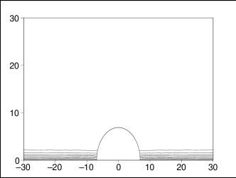
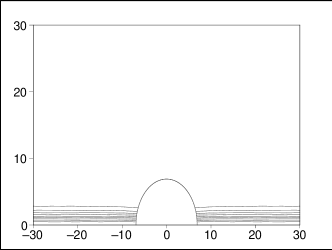
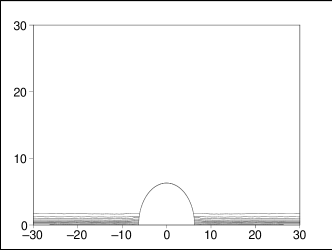
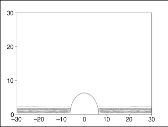
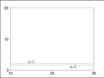
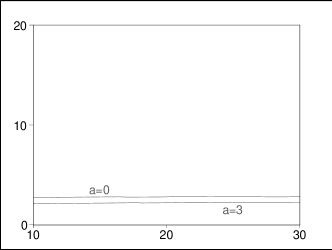
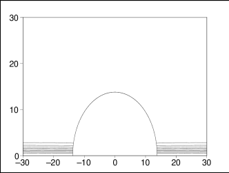
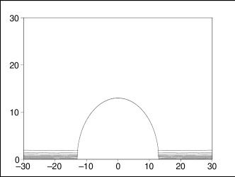
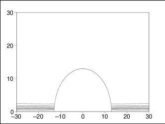
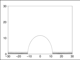
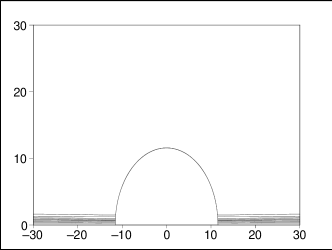
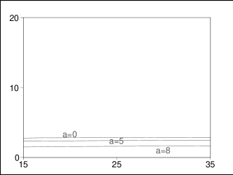
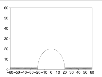
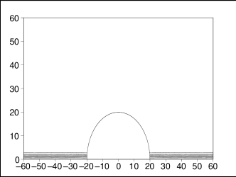
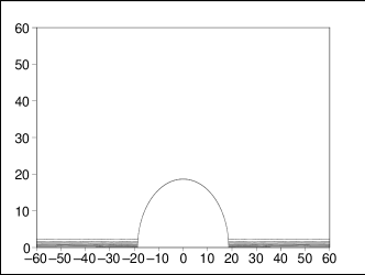
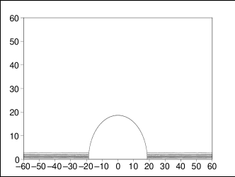
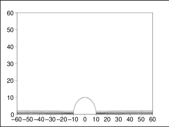
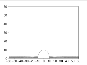
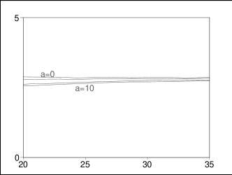
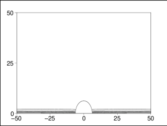
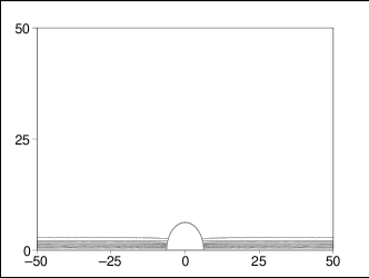
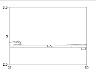
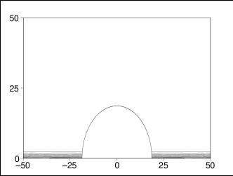
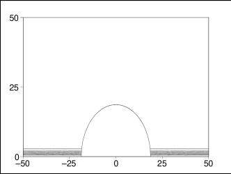
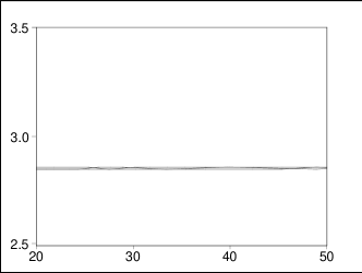
Some typical results of this calculation are displayed in figures (1), (2) and (4),(5), (6) for different
values of and , respectively. In the first case, we consider
both and and in the second case, we consider For , the black hole mass is taken to be the constant value whereas
for the mass is taken to be In the horizon is
located in for and for Also, for the
case of the horizon for different values of are respectively. For these two values of , the
black holes are non-extremal for all values of . The diagrams (1) and (4) when are exactly the same as the results of [13] for the AdS-Schwarzschild black hole. We notice that by increasing
the rotation parameter from to the string core decreases
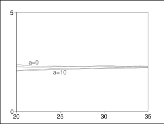
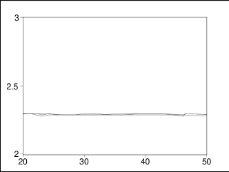
slightly in the Kerr-AdS black hole. Figure (3) shows
explicitly the string core decreasing as the rotation parameter increases.
The physical reason for the core size decreasing with increasing rotation
parameter is due to a decrease in the horizon radius . This
quantity is given by the root of equation (3) and decreases
slowly as the parameter increases from to its maximum value. On
the other hand, since we know from previous work that the string thickness
compared to horizon radius drastically changes by changing unbounded
physical quantities like the winding number or black hole mass, we expect
that string core changes a little with changing the bounded black hole
parameters like the rotation parameter . Since the effect of increasing (when ) is the same as the effect of decreasing on the value
of the horizon size we expect commensurate changes in the horizon
size. Indeed this is what we find: the core thickness increases with
decreasing parameter , analogous to what happens when the value of is
increased for .
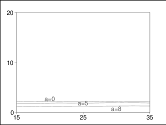
Figure (7) illustrates for a similar decrease of the string
core as increases from to and then to confirming again
our expectation. Our numerical results agree with the above statement
relating the horizon radius and different physical quantities of the black
hole. Similar calculations for the string with larger winding numbers in a
Kerr-AdS black hole with definite parameters , show that increasing the
winding number yields a greater vortex thickness.
For the extremal Kerr-AdS black hole with cosmological parameters mass and rotation parameter we have calculated the
vortex fields. In this case the horizon radius is located at We find that the behaviour of the vortex and fields are the same
as the non-extremal cases. The contours of the and fields attach
to the horizon in the same way they attach to the horizon of non extremal
black holes presented in the figures 1,2,4,5,6. Since the results are so similar to the non-extremal
cases we do not present them here. The crucial point is that in the extremal
case, no flux-expulsion is occurred in the thin vortex configuration.
4 Abelian Higgs Vortex in Reissner-Nordstrom-AdS and
Reissner-Nordstrom black holes
In this section, we consider the Abelian Higgs vortex Lagrangian (1)
in the background of a charged black hole. The background metric is given
by,
|
|
|
(24) |
is the total charge of black hole which measured by a far observer
located at and the black hole horizon is located at the largest real root of the equation In the special case of , the horizon is located at The Abelian Higgs Lagrangian is as the same as (1) with the real
fields again given by the
relations (5), whose equations of motion are (6) and
(7). The equations of motion derived from the Lagrangian for the and fields after rescaling of coordinates in
the background (24) are
|
|
|
|
|
(25) |
|
|
|
|
|
(26) |
We note that in the special case , the equations of motion (25) and (26) reduce to the equations of motion of the
vortex in the background of AdS-Schwarzschild background studied in [13]. Also we note that in the special case of
the above mentioned equations reduce to the equations of motion in the
background of the Reissner-Nordstrom black hole discussed in [6] and
[7].
We consider the static case of a string solution with winding number one.
Using the overrelaxation method described in section two, we solve
numerically the equations of motion. A typical result for the string fields
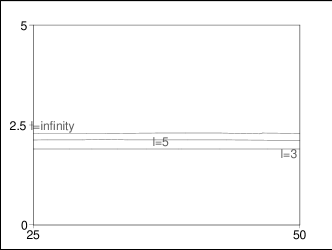
in the background of the Reissner-Nordstrom-AdS black hole with and is presented in figure (12). As figure (13) shows,
by increasing the parameter from to the string core
changes a little. Such a tiny increase of string core also has been observed
in the case of AdS-Schwarzschild black hole by increasing the parameter
[13]. In the special case of , a typical
solution of (25) and (26) for a Reissner-Nordstrom
black hole with and is shown in figure (14). In
figure (15), the and contours are plotted for three
different values of the charge parameter The last case
corresponds to extremal case So, we observe that despite the
smaller horizon radius for a black hole with more charge, the string core
does not change drastically for the charged black holes for a wide range of
the charge parameter . In the extremal case we find that an
extremal horizon is indeed pierced by a thin string, confirming earlier
computations carried out in references [8] and [9], and that the vortex flux is not expelled from the black hole. In these calculations,
we have used a grid in the directions, a much
finer resolution than employed in previous studies [6, 7, 8, 9].
Note that there are no values of or for which the black hole becomes
extremal in the asymptotically AdS case.
5 Vortex Self Gravity and Kerr Black Holes
In this section, we study the effect of the vortex on the Kerr black hole.
The Kerr metric (21) can be written in the axisymmetric Weyl
form as follows [16]:
|
|
|
(27) |
where the functions are independent of and
are given by,
|
|
|
(28) |
The quantities , and are given by
|
|
|
(29) |
The transformation between the spherical coordinates in (21)
and Weyl coordinates in (27) is given by,
|
|
|
(30) |
These Weyl coordinates are useful for studying the back reaction of the
vortex on the Kerr black hole.
In order to get the gravitational effect of the vortex on the Kerr black
hole, we consider a general static axisymmetric metric of the form
|
|
|
(31) |
where and are dependent on the Weyl coordinates
and The Einstein equations become
|
|
|
(32) |
|
|
|
(33) |
|
|
|
(34) |
|
|
|
(35) |
where and is the determinant of the metric
(31). The non-vanishing energy-momentum components are given by
|
|
|
(36) |
Writing where we can solve the equations (32)-(35) to first order in To order zero in the
background metric is give by (27) and the string fields by and So to first order in equation (32) becomes
|
|
|
(37) |
which can be solved by assuming the form Here,
we take Then function satisfies
|
|
|
(38) |
which can be solved to give
|
|
|
(39) |
Since outside the vortex core the string fields and
rapidly approach constant values, the integrals in (39) go
correspondingly to the respective constant values and This gives , and the
solutions of the other coupled equations (33)-(35) are
found to be and
where Using these
quantities in (31) and rescaling the coordinates
and function , by and we get
finally,
|
|
|
(40) |
which describes the Kerr metric with a deficit angle, since the angle belongs to the interval
6 Vortex Self Gravity on the Kerr-AdS and Reissner-Nordstrom-AdS
Black Holes
We now first consider the effect of the vortex on the Kerr-AdS black hole.
As we have seen in [13], this is a formidable problem even for the
simpler cases of the effect of the vortex on the AdS-Schwarzschild or
Schwarzschild black hole backgrounds.
For the AdS-Schwarzschild black hole, it has been shown that the components
of the energy-momentum tensor rapidly go to zero outside the core string,
leading to a situation similar to that of pure AdS spacetime. A full study
of vortex self gravity in pure AdS spacetime was carried out in ref. [13]. We assume for the present case that the thickness of the vortex is
much smaller than all other relevant length scales and that the
gravitational effects of the string are weak enough so that the linearized
Einstein-Abelian Higgs differential equations are applicable. So, we
consider a thin string with the winding number in the Kerr-AdS
background with . The analysis for other values of is similar. The
rescaled diagonal components of the energy-momentum tensor are
|
|
|
|
|
(41) |
where the functions and are
complicated functions of the coordinates Their
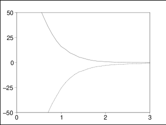
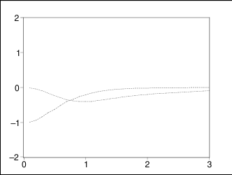
functional forms are presented in the appendix. In the figure (16)
the behaviour of energy-momentum tensor components for a fixed value of
is shown. We have checked that the behaviour of the components other
directions is similar.
It is clear from these figures that the components of the energy-momentum
tensor rapidly go to zero outside the core of the vortex, rendering the
situation similar to that of AdS-Schwarzschild spacetime. Performing the
same calculation as for pure AdS spacetime described in detail in [13], we obtain the following metric for the Kerr-AdS spacetime incorporating
the effect of the vortex
|
|
|
(42) |
which is a constant dependent on the different parameters of the
black hole. The above metric describes a Kerr-AdS metric with a deficit
angle. Also if we take the limiting case of we get
the following Kerr spacetime incorporated the effect of the string on it,
|
|
|
in which is another constant that also depends on the different
parameters of the Kerr black hole as noted above in (40).
So, using a physical Lagrangian based model, we have established that the
presence of the cosmic string induces a deficit angle in the Kerr-AdS and
Kerr black holes metric. In the case of charged Reissner-Nordstrom-AdS black
hole, the energy-momentum tensor also goes rapidly to zero outside the core
string, so the above arguments are still applicable: the effect of the
vortex on the background (24) simply multiplies the angle
coordinate by a constant, inducing a deficit angle in the
Reissner-Nordstrom-AdS black hole spacetime.
8 Appendix
Here we present the coefficients
appear in the equations (17) and (18). Let us
rename the coefficients of the and (fifth term) appearing in the equation
(10) by
respectively. Also, we rename the coefficients of the appearing in the equation (11) by respectively. Then the
coefficients inside the grid points are given by the
following relations,
|
|
|
The coefficients have the similar
form as with the replacements by and
|
|
|
The coefficient is equal to zero.
Here, we present also some of the functional form of the functions and which was appeared in the
formula (41).
|
|
|
Other functions have similar complicated structures; we shall not present
them here.
This work was supported by the Natural Sciences and Engineering Research
Council of Canada.