Bootstrap Methods in 1+1-Dimensional

Quantum Field Theories:

the Homogeneous Sine-Gordon Models

Olalla A. Castro Alvaredo^,

Departamento de Física de Partículas, Facultade de Física,

Universidade de Santiago de Compostela,

E-15706 Santiago de Compostela, Spain

Abstract

The bootstrap program for 1+1-dimensional integrable Quantum Field Theories (QFT’s) is developed to a large extent for the Homogeneous sine-Gordon (HSG) models. This program can be divided into various steps, which include the computation of the exact S-matrix, Form Factors of local operators and correlation functions, as well as the identification of the operator content of the QFT and the development of various consistency checks. Taking as an input the fairly recent S-matrix proposal for the HSG-models, we confirm its consistency by carrying out both a Thermodynamic Bethe Ansatz (TBA) and a Form Factor analysis, which allow for extracting the main characteristics of the underlying Conformal Field Theory (CFT) associated to these theories. In contrast to many other 1+1-dimensional integrable models studied in the literature, the HSG-models possess two remarkable features, namely the parity breaking, both at the level of the Lagrangian and S-matrix, as well as the presence of unstable particles in the spectrum. These features have specific consequences in our analysis which are given a physical interpretation. By exploiting the Form Factor approach, we develop further the QFT advocated to the HSG-models by evaluating correlation functions of various local operators of the model. We compute the renormalisation group (RG) flow of Zamolodchikov’s c-function and $\Delta$-functions which carry information about the RG-flow of the operator content of the underlying CFT and provide a means for the identification of the operator content of the QFT. For these functions, as well as for the scaling function computed in the TBA-context, an ‘staircase’ pattern which can be physically interpreted, by associating the different plateaux to energy scales for the onset of stable and/or unstable particles of the model, is found. For the $SU(3)_{2}$-HSG model we show how the form factors of different local operators are interrelated by means of the momentum space cluster property. We find closed formulae for all $n$-particle form factors of a large class of operators of the $SU(N)_{2}$-HSG models. These formulae are expressed in terms of universal building blocks which allow both a determinant and an integral representation.

SUPERVISOR

Prof. Dr. J.L. MIRAMONTES ANTAS,
Departamento de Física de Partículas, Universidade de Santiago de Compostela, Spain.

THESIS COMMISSION

Dr. P.E. DOREY,
Department of Mathematical Sciences, University of Durhan, England.

Dr. A. FRING,
Institut für Theoretische Physik, Freie Universität Berlin, Germany.

Prof. Dr. G. MUSSARDO,
International School for Advanced Studies, Trieste, Italy and
Istituto Nazionale di Fisica Nucleare, Sezione di Trieste, Trieste, Italy.

Prof. Dr. J. SÁNCHEZ GUILLÉN,
Departamento de Física de Partículas, Universidade de Santiago de Compostela, Spain.

Prof. Dr. G. SIERRA RODERO,
Instituto de Matemáticas y Física Fundamental, C.S.I.C., Madrid, Spain.

The original work presented in this PhD thesis, collects the results which can be found in the following publication list:

1. Decoupling the $SU(N)_{2}$-homogeneous sine-Gordon model.
   O.A. Castro-Alvaredo and A. Fring,
   Accepted for publication in Phys. Rev. D.
   hep-th/0010262. Chapter 5.
   

2. Renormalization group flow with unstable particles.
   O.A. Castro-Alvaredo and A. Fring,
   Phys. Rev. D63 (2001) 21701.
   hep-th/0008208. Chapter 4.
   

3. Identifying the Operator Content, the Homogeneous Sine-Gordon models.
   O.A. Castro-Alvaredo and A. Fring,
   Nucl. Phys. B604 (2001) 367.
   hep-th/0008044. Chapter 4.
   

4. Form factors of the homogeneous sine-Gordon models.
   O.A. Castro-Alvaredo, A. Fring and C. Korff,
   Phys. Lett. B484 (2000) 167.
   hep-th/0004089. Chapter 4.
   

5. Massive symmetric space sine-Gordon soliton theories and perturbed conformal field theory.
   O.A. Castro-Alvaredo and J.L. Miramontes,
   Nucl. Phys. B581 (2000) 643.
   hep-th/0002219. Chapter 2.
   

6. Thermodynamic Bethe ansatz of the homogeneous sine-Gordon models.
   O.A. Castro-Alvaredo, A. Fring, C. Korff and J.L. Miramontes,
   Nucl. Phys. B575 (2000) 535.
   hep-th/9912196. Chapter 3.
   

Chapter 1 Introduction

The study of 1+1-dimensional massive quantum field theories (QFT) has turned out to be a very fruitful research field for almost three decades. Various distinguished properties arising in the 1+1-dimensional context are responsible of this success and it is our intention to begin this thesis by providing a very brief glimpse of them through points I-IV:

I. Conformal invariance becomes in the 1+1-dimensional context an extremely powerful symmetry [1, 2, 3, 4]. In any dimension, conformal transformations are the subset of coordinate transformations which leave the metric invariant up to a local scale factor, namely

$$g_{\mu\nu}\rightarrow e^{\Lambda({x})}g_{\mu\nu}.$$

However, it turns out that only in 1+1-dimensions the conformal symmetry algebra becomes infinite dimensional, which means that there will be infinitely many conserved quantities associated to any 1+1-dimensional conformal field theory (CFT) . Consequently, conformal invariance becomes an extremely constraining requirement in the 1+1-dimensional context and many problems, which for general QFT’s can only be handled with great difficulties find an exact solution within the context of 1+1-dimensional CFT’s.

II.   Although it is more restrictive for 1+3-dimensional massive QFT’s, the so-called Coleman-Mandula theorem [5] is one of the key properties one has to appeal to in order to unravel the origin of the distinguished features of 1+1-dimensional massive QFT’s. The mentioned theorem was formulated and proven in 1967 by S. Coleman and J. Mandula [5]. These authors determined (under certain assumptions) the maximum S-matrix symmetry group associated to a 1+3-dimensional massive QFT. They found that for any local, relativistic, massive 1+3-dimensional QFT a symmetry group, $G$, containing the Poincaré group, $\mathcal{P}$, and an arbitrary internal symmetry group, $\mathcal{I}$, should necessarily be a direct product of the form

$$G=\mathcal{I}\otimes\mathcal{P},$$

Amongst all the hypothesis involved in the derivation of Coleman-Mandula theorem, it is worth emphasising that the symmetry group $G$ is assumed to be a Lie group whose generators obey a Lie algebra based on commutators. Alternatively, the theorem can be formulated by stating that, under the mentioned assumptions [5], space-time and internal symmetries can not be combined in any but a trivial way for 1+3-dimensional massive QFT’s.

III.  As mentioned above, the Coleman-Mandula theorem explicitly refers to the 1+3-dimensional domain. Nonetheless it has also a crucial counterpart in the 1+1-dimensional context. The result we are referring to can be formulated in very close spirit to the Coleman-Mandula theorem: the combination of space-time and internal symmetries in a non-trivial way is possible for 1+1-dimensional massive QFT’s. Equivalently, in 1+1-dimensions and assuming a purely massive particle spectrum, the existence of conserved quantities different from the energy, the space momentum, and the charges associated to internal symmetries does not force the S-matrix to be trivial. However, the S-matrix is constrained in a very severe way whenever the mentioned additional symmetries are present in the theory. In that case, the corresponding QFT is said to be integrable and the precise constraints we refer to are the following:

Absence of particle production in any scattering process.

‘Strict’ momentum conservation i.e., equality of the sets of momenta of incoming and outgoing particles.

Factorisability of all $n$-particle scattering amplitudes into $2$-particle ones.

Denoting by $S_{a_{1}\cdots a_{n}}^{b_{1}\cdots b_{k}}(p_{a_{1}},\cdots,p_{a_{n}};p_{b_{1}},\cdots,p_{b_{k}})$ the scattering amplitude of a process with $n$ incoming particles of quantum numbers $a_{1},\cdots,a_{n}$ and momenta $p_{a_{1}},\cdots,p_{a_{n}}$ and $k$ outgoing particles of quantum numbers $b_{1},\cdots,b_{k}$ and momenta $p_{b_{1}},\cdots,p_{b_{k}}$, the previous constraints can be expressed as

$$S_{a_{1}\cdots a_{n}}^{b_{1}\cdots b_{k}}(p_{a_{1}},\cdots,p_{a_{n}};p_{b_{1}},\cdots,p_{b_{k}})\propto\delta_{n,k}\prod_{i=1}^{n}\delta(p_{a_{i}}-p_{b_{i}})\equiv S_{a_{1}\cdots a_{n}}^{b_{1}\cdots b_{n}}(p_{1},\cdots,p_{n}),$$

$$S_{a_{1}\cdots a_{n}}^{b_{1}\cdots b_{n}}(p_{1},\cdots,p_{n})=\prod_{i<j,l<k}S_{a_{i},a_{j}}^{b_{k},b_{l}}(p_{i},p_{j}).$$

Such severe constraints to the form of the scattering amplitudes for integrable models were originally observed in the context of the study of various concrete 1+1-dimensional QFT’s [6]. In particular, the investigation of these models lead the different authors to conjecture the factorisability property mentioned above. Remarkably, a very analogous property had been already encountered much earlier in the non-relativistic framework (see e.g. [7]). The properties itemized above were thereafter reviewed in more generality by R. Shankar and E. Witten [8] and by D. Iagolnitzer in [9]. The arguments presented in those articles relied on the assumption of the presence of infinitely many conserved quantities in the QFT, in order to derive the outlined S-matrix constraints. Later, S. Parke refined the arguments in [8, 9] by showing in [10] that actually the presence of just two non-trivial conserved quantities in the theory leads to the same conclusions drawn in [8, 9]. The main arguments presented in [8, 9, 10] will be reviewed in chapter 2 of this thesis.

In the previous equations, the particles $a_{i},b_{i}$, for all values of $i=1,\cdots,n$ are particles belonging to the same mass multiplet. The conservation of the set of momenta of incoming and outgoing particles still allows for a possible exchange of quantum numbers between particles in the $in$- and $out$-states. This is possible whenever the particle spectrum is degenerate, namely there is more than one particle in each particle multiplet. In that case the S-matrix is said to be non-diagonal. However, for many interesting theories (in particular, the ones studied in this thesis) the mentioned degeneration does not occur and the two-particle scattering amplitudes can be written as

$$S_{a_{i},a_{j}}^{b_{k},b_{l}}(p_{i},p_{j})=\delta_{i}^{k}\delta_{j}^{l}S_{i,j}(p_{i},p_{j}),$$

which means that the corresponding S-matrix is diagonal and usually simplifies its explicit construction.

The constraints arising from integrability are also in the origin of the so-called Yang-Baxter [11] and bootstrap equations [12] which together with the physical requirements of unitarity, crossing symmetry, Hermitian analyticity, and Lorentz invariance of the scattering amplitudes [12, 13, 14, 15, 16, 17] allow in many cases for the exact calculation of the corresponding S-matrix. The main steps involved in such a construction as well as the nature of the properties summarised above will be analysed in detail in the next chapter.

IV.  A fundamental link between the properties stated in I and III was established by A.B. Zamolodchikov in [18]. This result has been extensively exploited in the study of 1+1-dimensional integrable QFT’s over the last decade and can be summarised as follows: a 1+1-dimensional QFT may be viewed as a perturbation of a CFT by means of a particular operator of the CFT itself. Equivalently, one could write formally the action functional associated to a 1+1-dimensional QFT as

$$S=S_{\text{CFT}}+\lambda\int d^{2}x\,\Phi(x,t),$$

for $S_{\text{CFT}}$ to be the action of the unperturbed CFT, $\lambda$ a coupling constant and $\Phi(x,t)$ a local field which in the ultraviolet limit corresponds to a local field of the CFT. In this fashion the unperturbed or underlying CFT is recovered in the ultraviolet limit of the perturbed CFT. Equivalently, the perturbation of the CFT breaks the original conformal invariance by taking the CFT away from its associated renormalisation group critical fixed point. Nonetheless, being the original conformal invariance extremely powerful it is to be expected that it has some ‘remaining’ counterpart in the massive QFT. Indeed, it was proven in [18] that for suitable choices of the perturbing field (we will see what this means in the next chapter), we will end up with a massive QFT which is not conformally invariant but still possesses an infinite number of conserved quantities and is therefore integrable in the sense of III. In order to prove the integrability of the model at hand, those conserved quantities can be explicitly constructed by doing perturbation theory around the original CFT or their existence may be proven by appealing to the so-called counting-argument presented in [18].

As a summary of the previous points I-IV, let us consider a 1+1-dimensional CFT for which, if we are fortunate, a lot of information will be available. We may perturb it by means of a certain local field of the CFT itself and construct this way a 1+1-dimensional massive QFT. Thereafter, by exploiting the methods mentioned in IV, we might be able to establish whether or not the perturbed CFT is integrable. In case the answer is positive the properties stated in III are automatically fulfilled namely, the latter QFT will be described by a factorisable S-matrix and there will be no particle production in any scattering process. Furthermore, the scattering amplitudes are forced to satisfy other requirements already mentioned in III, which may allow for the exact construction of the S-matrix associated to the massive QFT by carrying out the so-called bootstrap program [12]. It is important for later purposes to mention that, the outlined procedure often involves certain assumptions and ambiguities which are ultimately justified by the self-consistency of the results obtained. An example of the former is the extrapolation of semi-classical results to the QFT and, concerning the latter, any S-matrix proposal will be always determined up to certain factors, the so-called CDD-factors [19]. These factors are functions which do not add any physical information to the S-matrix proposal and satisfy trivially all the requirements summarised in III.

In the light of the previous observations, once a certain S-matrix has been constructed by means of the bootstrap program and assumed to describe the scattering theory associated to a certain 1+1-dimensional integrable QFT, it is highly desirable to develop tools which allow for consistency checks of this S-matrix proposal, that is, approaches which permit a definite one-to-one identification between the S-matrix constructed and the particular QFT under consideration. If the massive QFT has been constructed along the lines summarised in the preceding paragraph, its ultraviolet limit should lead to the original unperturbed CFT, whose main characteristics are

Virasoro central charge

Conformal dimension of the perturbing field

Local operator content

Therefore, having a certain perturbed CFT at hand, for which an S-matrix proposal has been constructed, we want to develop methods which taking this S-matrix proposal as an input allow for checking if it really corresponds to the specific massive QFT under study. Moreover, since the massive QFT has been constructed as perturbed CFT, such consistency checks may exploit the knowledge of the characteristics of the underlying CFT itemized above. These sorts of tools or approaches are commonly referred to as Bootstrap methods [12]. Amongst them, the thermodynamic Bethe ansatz (TBA) originally proposed by C.N. Yang and C.P. Yang in [20] and formulated in the present form by A.B. Zamolodchikov [21], and the form factor approach, pioneered in the late seventies by the Berlin group of the Freie Universität [22], constitute prominent examples. The purpose of the work presented in this thesis will be the application of these methods to the study of a concrete family of 1+1-dimensional massive integrable QFT’s together with the further investigation of the mentioned approaches themselves.

We do not want to describe in detail now the formulation of these two approaches, which will be done in subsequent chapters. Nonetheless, it is worth noticing here that both the TBA- and form factor approach take as an input the knowledge of the exact S-matrix associated to a certain 1+1-dimensional QFT and allow in principle for computing both the Virasoro central charge of the underlying CFT and the conformal dimension of the perturbing field. Moreover, in the TBA-context, the finite size scaling function [23] can be computed (usually numerically). The latter function can be understood for unitary CFT’s as a sort of ‘off-critical’ Virasoro central charge which measures the amount of effective light degrees of freedom present in the theory at each energy scale. Such a function has a counterpart which is expressible in terms of correlation functions involving different components of the energy momentum tensor and is known as Zamolodchikov’s $c$-function [24]. It carries the same physical information as the finite size scaling function and both functions turn out to be qualitatively very similar, despite the fact, that their precise relationship is still an outstanding problem. The computation of Zamolochikov’s $c$-function will be possible within the form factor framework, since the knowledge of the form factors associated to a certain local operator allows for the computation of its two-point correlation function.

Moreover, it must be emphasised that the form factor approach goes, at least at present, beyond the previous applications and, in contrast to the TBA-analysis, allows also for the further development of the QFT advocated to a certain model. In particular, as noticed above, the knowledge of the form factors associated to any local operator of the QFT allows for the computation of correlation functions involving such operator. The latter use of form factors can be exploited, for instance, in re-constructing at least a large part of the local operator content of the underlying CFT (apart from the perturbing field) by assuming a one-to-one correspondence between the local operator content of the unperturbed and perturbed CFT. Such correspondence can be established by evaluating the ultraviolet conformal dimensions of local operators of the massive QFT, that is, the conformal dimensions of those primary fields of the underlying CFT which are identified as their counterpart in the UV-limit. In order to carry out this identification we can consider the UV-limit of the two-point functions of local operators of the QFT, and extract thereafter the associated conformal dimension. Alternatively, in the form factor framework, $\Delta$-sum rules, like the one proposed in [27] which requires the knowledge of the two-point function of the local operator at hand and the trace of the energy momentum tensor, can be numerically evaluated for the ultraviolet conformal dimensions of certain local fields of the QFT.

The identification of the conformal dimensions of certain local operators of the underlying CFT, different from the perturbing field, can also be carried out in the TBA-context. This requires the re-formulation of this approach in order to extract the energies of excited states of the QFT, instead of the ground state energy available in the standard TBA-framework. These energies can be related thereafter to the conformal dimensions of certain operators of the underlying CFT. Work in this direction was first carried out in [25], where models whose ground state becomes degenerated for large volume were studied. Later in [26], the energies of excited states have been found to be obtainable via the analytical continuation to the complex plane of the parameters entering the standard TBA-equations. Unlike as in the form factor context described above, the latter “excited TBA” analysis still does not provide a direct mechanism which allows for matching the operator contents of the perturbed and unperturbed CFT. Instead, this analysis allows, in principle, for reconstructing the Hilbert space of the theory at different energy scales (system sizes), providing therefore a map between energy eigenstates in the UV- and IR-limits. In the form factor context, the $\Delta$-sum rule proposed in [27] can be modified by introducing a dependence on the RG-parameter, as shown in [28] in such a way that we can now reconstruct the operator content of the theory at different energy scales, as we show in particular for the HSG-models in this thesis. In that context, we will compute quantities which we could name as “off-critical” conformal dimensions $\Delta(r)$, whose variation in terms of the RG-parameter from the UV- to the IR-regime, reproduces the renormalisation group flow of the operator content of the theory in terms of the RG-energy scale.

Having now introduced the main ideas entering the study we will present in this thesis, what is left is the description of the concrete theories for which the TBA- and form factor analysis will be carried out. These theories are particular examples of the large family of Toda field theories [29] which arise as field generalisations of one of the simplest classically integrable models: the Toda lattice [30, 31]. The Toda lattice is a discrete mechanical system consisting of a set of $n$ particles located along a line and characterised by non-linear interactions. In fact, as shown in the picture at the end of this chapter, it is usual to distinguish between the Toda lattice and Toda molecule, to indicate that in the $n$-particle system mentioned above the two particles on the extremes are coupled to a solid wall (lattice) or that this wall is ‘taken to infinity’ (molecule) and, in that sense, there are no boundaries. A precursor of these models was studied by E. Fermi, J. Pasta and S. Ulam in [32] in the course of a numerical simulation to study heat conductivity in solids and their field generalisations gave rise to the large family of theories whose main features shall be itemize below. The mentioned generalisation is carried out by adding to the original discrete coordinates $q_{i}(t)$, $i=1,\cdots,n$, a space dependence of the form $q_{i}(x,t)$. Thereafter, the latter functions can be naturally arranged into a field, $h(x,t)$ which takes values in a certain Lie algebra, $g$. If the field takes values in the Cartan subalgebra of $g$, the corresponding theories are known as abelian Toda field theories. These theories have been extensively studied in the literature and can be further classified into the three following groups:

If the Lie algebra $g$ is finite, the corresponding abelian Toda field theories are known as conformal Toda field theories [29]. As their name indicates, they are conformally invariant. The simplest example of this type of theories is Liouville’s theory.

If the Lie algebra is an affine Kac-Moody algebra (affine extension of $g$ without central extension), the resulting theories are known as affine Toda field theories (ATFT). These are massive QFT’s which may be understood, following point IV, as perturbations of the class of conformally invariant models introduced in the previous paragraph. Amongst these theories, we encounter two very different groups depending whether the associated coupling constant, $\beta$ is real or purely imaginary. In the former case, the corresponding models do not possess solitonic solutions at classical level and their description, although well established in the infrared limit, is problematic in the ultraviolet regime. These theories constitute examples of 1+1-dimensional QFT’s which have been most extensively studied in the literature, first on a case-by-case basis, both for simply laced Lie algebras [33, 34, 35, 36, 37] and for the non simply-laced case [38]. Eventually, universal representations for the S-matrices valid for all simply laced ATFT’s with real coupling constant in form of hyperbolic functions [39] and integral representations valid for all ATFT’s [40, 41] based on purely algebraic quantities, were formulated thereafter (see also [42]). However, a rigorous proof of the equivalence between the S-matrix representation in terms of hyperbolic functions and the integral representation for all ATFT’s was first carried out in [41]. The simplest example of ATFT’s is the sinh-Gordon model [43, 44]. Concerning ATFT’s associated to purely imaginary coupling constant, one of its most relevant features is the existence of solitonic solutions. The infrared description of such theories involves in general non-unitary S-matrices but their ultraviolet limit is better established than for the ATFT’s with real coupling constant mentioned before. The simplest and best known example of this class of models is the sine-Gordon model ($SU(2)$-ATFT) even though scattering matrices corresponding to other choices of the Lie algebra have been also constructed in [45].

Finally, the last example of abelian Toda field theories are the so-called conformal affine Toda field theories [46], which may be obtained from the affine Toda field theories by introducing auxiliary fields $\eta,\mu$ in order to restore conformal invariance. They can also be defined as those conformal theories whose spontaneous symmetry breaking leads to the affine Toda field theories defined above.

On the other hand, when the field $h(x,t)$ takes values in a non-abelian Lie algebra $g$, a new rich family of models emerges. These models are known as non-abelian Toda field theories (NAAT) [47] and a particular subset of them will be the final object of our study. The NAAT-theories were originally constructed as non-abelian generalisations of the abelian Toda field theories described above. Such a generalisation can be carried out in different ways. The original construction due to A.N. Leznov and M.V.  Saveliev (see first reference in [47]) associates different types of equations of motion to each possible embbeding of $sl(2,\mathbb{C})$ into the non-abelian Lie algebra $g$. However, a systematic and more general description of the NAAT-theories was carried out in the two last references in [47] and in [48]. The mentioned construction associates different types of equations of motion to each possible gradation of an affine Lie algebra $\hat{g}$ associated to a finite semisimple Lie algebra $g$. This gradation is induced by a finite order automorphism of $g$, usually denoted by $\sigma$ [48]. However, it is worth mentioning that the explicit use of affine Lie algebras is not needed but when one attempts to explicitly construct higher spin conserved quantities.

Although all NAAT-theories are classically integrable, it was shown in [48] that at quantum level only two particular subsets of NAAT-theories can be associated with unitary and massive QFT’s. These two families of theories were named in [48] as homogeneous sine-Gordon models (HSG) and symmetric space sine-Gordon models (SSSG). The latter two subsets of NAAT-theories are of special interest since, remarkably, they simultaneously possess classical solitonic solutions, their ultraviolet description is well established and they are expected to admit also an infrared description in terms of unitary S-matrices, which have been explicitly constructed in [51] for the HSG-models corresponding to simply-laced Lie algebras.

The HSG-models have been studied to quite a large extent by members of the Theory group of the University of Santiago de Compostela (Spain) along the last years [48, 49, 50, 51, 52, 53]. This study gave rise ultimately to an S-matrix proposal for all the HSG-models associated to simply-laced Lie algebras [51] which constitutes the starting point of the whole analysis presented in this thesis. The development of consistency checks for this S-matrix proposal has been one of the main aims of the work presented here.

The action associated both to the HSG- and SSSG-models may be written in the general form

$$S=S_{WZNW}+\frac{m^{2}}{\pi\beta^{2}}\int d^{2}x\,\langle\Lambda_{+},h^{\dagger}\Lambda_{-}h\rangle,$$

where the first term is the action of a Wess-Zumino-Novikov-Witten (WZNW) [57, 58] coset model, associated to a coset of the general form $G_{0}/U(1)^{p}$. $G_{0}$ is the Lie group associated to a compact finite and semisimple Lie algebra $g_{0}\subset g$ and $p$ is an integer whose value depends on the particular type of theories under study. The WZNW-models [57, 58] are conformally invariant theories so that the HSG- and SSSG-models may be understood as perturbed CFT’s in the sense described in IV. The perturbing field is identified in that case to be $\Phi=\langle\Lambda_{+},h^{\dagger}\Lambda_{-}h\rangle$ where $\Lambda_{\pm}$ are two semisimple elements of $g$ and $\langle\,,\,\rangle$ denotes a bilinear form in $g$.

For the HSG-models $g_{0}=g$ and the integer $p$ equals the rank of the Lie algebra $g$, which we will denote by $\ell$. Therefore, they are perturbations of WZNW-coset models associated to cosets of the form $G_{k}/U(1)^{\ell}$ which are also known in the literature as $G_{k}$-parafermion theories. Here we introduced an integer $k$ that is called the ‘level’ [57, 58] and in terms of which the coupling constant $\beta^{2}$ gets quantized for the quantum theory to be well-defined. The main characteristics of these CFT’s have been studied in [59, 60, 61] and, in particular, their local operator content is well classified, a fact which we might exploit in the context of our form factor analysis. Finally, the elements $\Lambda_{\pm}$ characterising the perturbing field take values in the Cartan subalgebra of $g$. The simplest example amongst the HSG-models is associated to $g=su(2)$ and can be identified with the so-called complex sine-Gordon model [62, 63]. This theory corresponds to the perturbation of the usual $\mathbb{Z}_{k}$-parafermions [64] by the first thermal operator [65], whose exact factorisable scattering matrix is the minimal one associated to $A_{k-1}$ [64, 33].

As mentioned above, recently an S-matrix proposal for all HSG-models related to simply-laced Lie algebras has been provided in [51]. These S-matrices include some novel features with respect to many other integrable QFT’s which is worth emphasising already at this point: they break parity invariance, they have resonance poles which may interpreted as the trace of the presence of unstable particles in the model and they posses at the same time a well-defined Lagrangian description. Although in [54] the SSSG-models associated to the symmetric space $SU(3)/SO(3)$ were first investigated and found to be quantum integrable and to possess the above mentioned properties, an S-matrix proposal for these concrete theories is absent for the time being. Therefore, the S-matrices constructed in [51] for the HSG-models still provide the first examples of scattering amplitudes which having a non-trivial rapidity dependence, incorporate consistently parity breaking together with the presence of unstable particles in their spectrum.

Concerning the SSSG-models, some of their characteristics have been studied in [56, 55] despite the fact that little information is known in comparison to the above mentioned HSG-models. In particular, the development of an S-matrix proposal is an open problem for the time being for all SSSG-theories. However, part of their classical soliton spectrum was constructed in [56] and also the quantum integrability of a subset of them proven. We will devote part of the next chapter to a more detailed description of the results obtained in [56] for these models.

The SSSG-theories are in one-to-one correspondence with the compact symmetric spaces $G/G_{0}$ [66] which also means that the Lie algebra $g$ associated to $G$ admits a decomposition of the form $g=g_{0}\oplus g_{1}$. Here $g_{0}$ is a subalgebra of $g$ whereas $g_{1}$ is a certain subspace of $g$ in which the elements $\Lambda_{\pm}$ take values. These theories are perturbations of WZNW-coset models associated to cosets of the form $G_{0}/U(1)^{p}$, where the value of $p$ is now not fixed but can take a certain range of values which is determined by the properties of the elements $\Lambda_{\pm}$. In particular there are two specially interesting situations:

$p=0$ : in that case the corresponding SSSG-model is just an integrable perturbation of the WZNW-theory associated to the Lie group $G_{0}$. These models have been called split models in [56, 55].

$p=\ell_{0}$: in that case the corresponding model is a perturbation of a WZNW-coset theory associated to a coset of the form $G_{0}/U(1)^{\ell_{0}}$, for $\ell_{0}$ to be the rank of $G_{0}$. Therefore we have new integrable perturbations of $G_{0}$-parafermion theories, different from the ones provided by the HSG-models.

The simplest examples of SSSG-models are the sine-Gordon model, which corresponds to the symmetric space $G/G_{0}=SU(2)/SO(2)$ and again the complex sine-Gordon theory which is now related to the symmetric space $Sp(2)/U(2)$. Also the SSSG-theories related to the symmetric space $SU(3)/SO(3)$ have been studied by V.A. Brazhnikov in [54]. In particular, for $p=1$, the perturbed CFT associated to the latter coset corresponds again to the perturbation of the usual $\mathbb{Z}_{k}$-parafermion theories [64], in this case by the second thermal operator.

Having now presented the key ideas entering the work we will carry out in this thesis, as well as the main defining characteristics of the homogeneous sine-Gordon models [48, 49], we will now summarise the content of each of the subsequent chapters:

In chapter 2 we will provide a fairly detailed revision of the most relevant properties of 1+1-dimensional QFT’s. In particular, since these properties are closely linked to the powerful nature of conformal invariance in the 1+1-dimensional context, we will start the chapter with a review of some of the most important properties of 1+1-dimensional CFT’s. Thereafter, we will enter the analysis of the properties of massive QFT’s constructed as perturbed CFT’s along the lines of [18]. We will also summarise the arguments presented in [8, 10], concerning the distinguished features of the scattering amplitudes of 1+1-dimensional integrable QFT’s mentioned in III. We will analyse the constraints any scattering amplitude is subject to in virtue of Lorentz invariance, unitarity, Hermitian analyticity and crossing symmetry and describe the link between the pole structure of the S-matrix and the stable and unstable particle content of the QFT [12, 13, 14, 15, 16, 17]. After this general part we will enter the analysis of the main properties of the non-abelian affine Toda field theories (NAAT) [47] paying special attention to the description of the classical and quantum aspects of the subset of these theories known under the name of homogeneous sine-Gordon models (HSG) [48, 49]. In particular, we will present in detail the semi-classical construction of their stable particle spectrum carried out in [50], as well as the S-matrix proposal of [51]. These data will constitute the starting point of the analysis carried out in the next chapters. We also present in this chapter a revision of some of the most relevant aspects of the symmetric space sine-Gordon models (SSSG) investigated in [55, 56]. Finally, we provide the reader with a brief overview of the characteristics of the $g|\tilde{g}$-theories proposed in [67], whose S-matrices have been constructed as generalisations of the HSG-model and minimal ATFT [33] S-matrices and, therefore, contain the latter as particular examples.

In chapter 3 we will introduce the fundamental ideas entering the thermodynamic Bethe ansatz approach (TBA) [20, 21] and carry out a TBA-analysis for the HSG-models [48, 49, 50, 51]. Our TBA-analysis will permit the identification of the Virasoro central charge of the underlying CFT for all the HSG-models. Also, the conformal dimension of the perturbing field will be identified by conjecturing its relation to the periodicities of the so-called $Y$-systems [139]. The finite size scaling function and $L$-functions entering the TBA-equations will be numerically computed for some particular examples of the $SU(3)_{k}$-HSG models, corresponding to $k=2,3$ and 4 and different values of the resonance parameter characterising the mass of the unstable particles present in the model. The original results presented in this chapter can be found in [68] (see also [69, 70, 71]).

In chapter 4 we will present the fundamental properties and applications of form factors to the study of 1+1-dimensional QFT’s and carry out a form factor analysis for the $SU(3)_{2}$-HSG model. We will introduce the consistency equations derived originally in [22], whose solution leads to the exact computation of the form factors associated to a certain local operator of the QFT, that is, matrix elements of the mentioned operator between the vacuum state and an $n$-particle $in$-state. Thereafter, we will discuss in total generality the applications of these form factors to the computation of different interesting quantities: the Virasoro central charge of the underlying CFT, Zamolodchikov’s $c$-function [24], the conformal dimensions of various local operators of the underlying CFT, the renormalisation group flow of the operator content of the underlying CFT, etc…After this general introduction we will carry out a detailed form factor analysis for the $SU(3)_{2}$-HSG model. We shall construct all $n$-particle form factors associated to a large class of local operators of the model in terms of general building blocks which admit both a determinant and an integral representation. We will identify the ultraviolet conformal dimensions of these operators by exploiting the knowledge of the operator content of the underlying CFT. We will also compute the Virasoro central charge of the unperturbed CFT and identify the conformal dimension of the perturbing field. We will numerically determine Zamolodchikov’s $c$-function [24] and generalise the $\Delta$-sum rule proposed in [27] to the ‘off-critical’ situation. We shall also analyse in detail the so-called momentum space cluster property of form factors for the model at hand. The original results presented in this chapter collect the work published in [72, 73, 28] (see also [71]).

In chapter 5 we will generalise the study of the previous chapter to all $SU(N)_{2}$-HSG models. We shall also construct all $n$-particle form factors associated to a large class of operators of the model finding again the same sort of building blocks encountered in the $SU(3)_{2}$-case. We will compute the Virasoro central charge, Zamolodchikov’s $c$-function and the conformal dimension of the perturbing field for several concrete values of $N$. We will also study the renormalisation group flow of the operator content of the underlying CFT and define what we have called $\beta$-like functions in order to have a clear-cut identification of the different fixed points both the $c$- and $\Delta$-function surpass in their flow from the ultraviolet to the infrared regime. The original work presented in this chapter may be found in [74].

In chapter 6 we will summarise the main conclusions of the work carried out in this thesis and state some open problems which are left for future investigations.

In appendix A we collect some useful properties of elementary symmetric polynomials.

In appendix B we present the explicit expressions of the form factors associated to a large class of operators of the $SU(3)_{2}$-HSG model up to the 8-particle form factor.

Chapter 2 1+1-dimensional integrable massive quantum field theories

In the previous introduction we provided a first glimpse of the distinguished properties of 1+1-dimensional integrable quantum field theories (QFT’s). Our aim was to furnish an introductory justification for the enormous interest that these sort of models have achieved over the last 30 years. In particular, we introduced the Toda field theories as a especially prominent class of QFT’s included in the previous category. We also reported very briefly the main properties of 1+1-dimensional integrable QFT’s and emphasised their consequences, in particular, in what concerns the construction of exact S-matrices.

The aim of the present chapter will be first, a more detailed analysis and derivation of the properties of 1+1-dimensional integrable QFT’s: their construction, the special characteristics of their S-matrices, and the general procedure which may allow for the exact construction of these S-matrices on the basis of a series of physical requirements together with the concrete constraints due to integrability. Second, we want to use the previous general results and techniques for the study of a concrete family of 1+1-dimensional integrable QFT’s, a subset of the non-abelian affine Toda (NAAT) field theories [47, 48]. In particular, we will pay special attention to a subclass of the latter theories, the homogeneous sine-Gordon (HSG) models [49], whose study, has been carried out to a large extent by the Theory group of the University of Santiago de Compostela (Spain), over the last years [48, 49, 50, 51, 52, 53]. The development of non-perturbative tests of the S-matrix proposal provided in [51] for those theories is one of the main objectives of the work we will present in this thesis. However, it must be emphasised that our results constitute also a valuable contribution to the understanding of several aspects related to the thermodynamic Bethe ansatz and form factor approach themselves.

In addition, we will also provide in this chapter original results [56] concerning the quantum properties of a second family of theories, the symmetric space sine-Gordon (SSSG) models [48, 55], which are also particular examples of massive NAAT-theories and whose study, for the time being, has not been carried out to such an extent as for the HSG-theories. Even the construction of exact S-matrices related to the SSSG-models is still a completely open problem. However, since the main objectives of this thesis are the ones stressed in the previous paragraph, we will not present here in detail the results found in [56].

More concretely, the structure of the present chapter will be the following:

In section 2.1 we shall present a brief overview of the main properties of conformally invariant theories [3, 4], necessary for the understanding of the more relevant characteristics of perturbed CFT’s. Recall that it was pointed out by A.B. Zamolodchikov in [18] that a 1+1-dimensional QFT may be viewed as a perturbation of a CFT which takes the latter away from its associated renormalisation group fixed point. The results provided in [18] will be reviewed in subsection 2.1.2. Thereafter, in section 2.2, we will analyse the specific properties of 1+1-dimensional integrable QFT’s, paying special attention to their consequences in what concerns the exact computation of S-matrices. After the introduction of the so-called Zamolodchikov’s algebra [16] in subsection 2.2.1 as a means for representing the asymptotic states in a 1+1-dimensional QFT, we will present the definition and properties of the so-called higher spin conserved charges. We shall explain how their existence in 1+1-dimensional QFT’s leads to the conclusion that the corresponding S-matrix factorises into products of two particle S-matrices and that there is no particle production in any scattering process [8, 9, 10]. In section 2.3 we shall summarise the specific properties of two-particle scattering amplitudes in 1+1-dimensional QFT’s [12, 13, 14, 15, 16, 17]. These properties are Lorentz invariance, Hermitian analyticity, unitarity and crossing symmetry together with two sets of highly non-trivial equations known as Yang-Baxter [11] and bootstrap equations [12, 13]. The first set of properties have their origin in physically motivated requirements whereas the latter two equations exploit the specific consequences of quantum integrability or the existence of higher spin conserved charges in the QFT. All these constraints allow in many cases for the exact computation of the S-matrix associated to a 1+1-dimensional QFT by means of the bootstrap program, originally proposed in [12]. We will also pay attention in section 2.3 to the pole structure of the two-particle scattering amplitudes, and report its intimate connection with the stable and unstable particle spectrum of the model at hand. Once the general framework and techniques have been reported, we will turn in section 2.4 to the description of the specific theories we will focus our interest on: the non-abelian affine Toda (NAAT) field theories [47]. After a very brief review on classical integrability, we will go through the quantum properties of all NAAT-theories, studied in [48, 49, 50, 63, 90, 52, 53, 51], exploiting the general results of sections 2.1, 2.2 and 2.3. In particular, we will describe in detail the characteristics of the two families of unitary and massive NAAT-theories found in [48]: the symmetric space (SSSG) and homogeneous sine-Gordon (HSG) theories. Since the latter models have been studied to a larger extent than the former and most of the original results presented in this thesis are related to the HSG-models, we will pay more attention to the description of the properties of these theories, and ultimately report the S-matrix proposal for the HSG-models related to simply-laced Lie algebras derived in [51]. We will also dedicate subsection 2.4.3 to a brief description of the properties of the SSSG-models, report the most prominent results obtained in [56] and provide arguments in order to motivate the interest of their further investigation. Finally, we will recall some of the features of a new type of S-matrices proposed in [67] which contain the HSG-models [49] and minimal ATFT [33, 34] as particular distinguished examples and whose underlying CFT was studied in [61]. These are the $g|\tilde{g}$-theories proposed by A. Fring and C. Korff in [67] for $g$, $\tilde{g}$ to be simply laced Lie algebras and recently generalised by C. Korff in [80] for the case when $\tilde{g}$ is non-simply laced.

2.1 From conformal field theory to massive quantum field theory

As outlined above, since in 1989 A.B. Zamolodchikov [18] pointed out that a 1+1-dimensional integrable QFT may be formally viewed as a perturbation of a CFT by means of a certain relevant field of the CFT itself, the latter approach has been successfully exploited by many authors in the course of the construction, classification and characterisation of 1+1-dimensional QFT’s. In the spirit of [18], the original ultraviolet CFT plays the role of starting point in the construction of a 1+1-dimensional massive integrable QFT. The key idea is that a CFT can always be thought of as a renormalisation group (RG) critical fixed point (see e.g. [4]). Therefore, its perturbation by means of any relevant operator amounts to “moving” the CFT away from its associated RG-fixed point and consequently, to breaking the initial conformal invariance. For arbitrary choices of the perturbing field one would expect to end up with a 1+1-dimensional QFT which, in general, may be neither conformal invariant nor integrable in the sense of possessing an infinite number of integrals of motion. However, the combination of a suitable choice of the perturbation together with the fact that conformal symmetry is an extremely high symmetry which provides every CFT with an infinite number of local conserved quantities, allows for the construction of 1+1-dimensional QFT’s which, although breaking conformal invariance still have associated an infinite number of conserved quantities. These conserved quantities arise as particular combinations of those of the original unperturbed CFT and may even be explicitly constructed along the lines of [18]. This construction has been carried out for instance for the mentioned HSG- and some SSSG-models in [49] and [56] respectively, aiming to prove their integrability. However, it is worth mentioning that the integrability of the perturbed CFT, is guaranteed by the existence of such quantities. This means that their explicit construction is not necessary in order to prove the integrability of the model whenever their existence can be established by other means. In this direction, it is possible to resort to the so-called “counting-argument” developed also by A.B. Zamolodchikov in [18], which will be described in detail later. The mentioned argument provides a sufficient condition for the existence of conserved quantities in a perturbed CFT and can be worked out provided the characters of the irreducible representations of the Virasoro algebra (see subsection 2.1.1) associated to the unperturbed CFT are known. As we said this criterium is sufficient to prove the existence of conserved charges in the massive QFT. To our knowledge, the mentioned characters are not known up to now for the generality of the underlying CFT’s related to the HSG- and SSSG-models, which is the reason why the explicit construction of some conserved quantities has been necessary for establishing their integrability.

The above qualitative arguments justify the important role CFT plays in the construction of 1+1-dimensional integrable QFT’s, of which the non-abelian affine Toda field theories [47] at hand are particular examples. We will devote the next subsection to the introduction of some basic notions on conformal field theory necessary for the subsequent understanding of the most relevant features of perturbed conformal field theory. Some of these properties will also be recovered both in the thermodynamic Bethe ansatz and form factor context since the application of any of these approaches to the study of 1+1-dimensional integrable models allows ultimately for the identification of the main data characterising the CFT which describes the ultraviolet behaviour of the QFT at hand.

2.1.1 Conformal field theory: a brief overview

In the light of the previous paragraph and to achieve self-consistency we will now introduce some basic notions on 1+1-dimensional conformal field theory. A more exhaustive discussion and derivation of these properties may be found for instance in [3, 4].

The classical conformal group

The conformal group in arbitrary dimension $d$ is the subset of coordinate transformations which leave the metric $g_{\mu\nu}$ invariant up to a scale transformation, namely

$$g_{\mu\nu}\rightarrow e^{\Lambda(x)}g_{\mu\nu}.$$ (2.1)

It can be proven by considering initially infinitesimal transformations of the type $x_{\mu}\rightarrow x_{\mu}+\epsilon_{\mu}$, that conformal symmetry requires

$$\partial_{\mu}\epsilon_{\nu}+\partial_{\nu}\epsilon_{\mu}=\frac{2}{d}\partial_{\rho}\epsilon^{\rho}\,\eta_{\mu\nu}$$ (2.2)

provided we consider a flat metric $g_{\mu\nu}=\eta_{\mu\nu}$. In this thesis we will be interested in the 1+1-dimensional case. Hence, the latter equation gives

$$\partial_{1}\epsilon_{1}=\partial_{2}\epsilon_{2},\,\,\,\,\,\,\text{and}\,\,\,\,\,\,\partial_{1}\epsilon_{2}=-\partial_{2}\epsilon_{1},$$ (2.3)

which, according to the Cauchy-Riemann theorem, suggests the definition of two new functions $\epsilon(z)$ and $\bar{\epsilon}(\bar{z})$ depending upon the complex coordinates $z,\bar{z}=x^{0}\pm ix^{1}$ as follows,

$$\epsilon(z)=\epsilon_{1}+i\epsilon_{2},\,\,\,\,\,\,\text{and}\,\,\,\,\,\,\bar{\epsilon}(\bar{z})=\epsilon_{1}-i\epsilon_{2}.$$ (2.4)

This result amounts to the conclusion that 1+1-dimensional conformal transformations are just analytic coordinate transformations in the complex plane of the form,

$$z\rightarrow f(z),\,\,\,\,\,\,\,\,\,\,\,\,\text{and}\,\,\,\,\,\,\,\,\,\,\,\,\bar{z}\rightarrow\bar{f}(\bar{z}).$$ (2.5)

The algebra which generates the sort of transformations (2.5) is infinite dimensional and the corresponding infinitesimal generators are found to be

$$l_{n}=-z^{n+1}\partial,\,\,\,\,\,\,\,\,\,\,\,\,\text{and}\,\,\,\,\,\,\,\,\,\,\,\,\bar{l}_{n}=-\bar{z}^{n+1}\bar{\partial},$$ (2.6)

with $\partial:=\partial/{\partial z}$ and $\bar{\partial}:=\partial/{\partial\bar{z}}$ and $n\in\mathbb{Z}$. These generators satisfy the Witt algebra,

$$\left[l_{n},l_{m}\right]=(m-n)l_{n+m},\,\,\,\,\,\,\left[\bar{l}_{n},\bar{l}_{m}\right]=(m-n)\bar{l}_{n+m},$$ (2.7)

with $\left[l_{n},\bar{l}_{m}\right]=0$ for any value of $n,m$. Therefore, the conformal algebra is the direct product of two isomorphic subalgebras generated by the $l$’s and the $\bar{l}$’s. At the quantum level, these commutation relations acquire an additional constant contribution on the r.h.s., giving rise to a so-called Virasoro algebra.

Having (2.6) at hand one easily observes that in the limits $z\rightarrow 0,\infty$ only the infinitesimal generators $l_{0},l_{\pm 1}$ are globally well defined and similarly for their anti-holomorphic counterpart. Moreover, Eq. (2.7) shows that their commutation algebra closes and is isomorphic to $sl(2,\mathbb{C})/\mathbb{Z}_{2}$. It might also be easily derived that $l_{-1},\bar{l}_{-1}$ are the generators of translations ($z\rightarrow z+a$) whereas $l_{0}+\bar{l}_{0}$ and $i(l_{0}-\bar{l}_{0})$ generate dilatations ($z\rightarrow\lambda z$) and rotations ($z\rightarrow e^{i\theta}z$) respectively.

Conformal symmetry at quantum level

Over the last 30 years, conformal field theory has became one of the most active and fruitful research fields in the context of mathematical physics. The explanation of this success relies on the fact that conformal invariance turns out to be an extremely powerful symmetry in 1+1-dimensions since, only in that case it is associated to an infinite number of independent generators. Consequently, many problems which can only be handled with great difficulties for general QFT’s find in this context an exact solution. In the framework of physical systems characterised by local interactions, conformal invariance can be understood as an immediate consequence of scale invariance. This observation was originally made by A.M. Polyakov [75]. Thereafter there have been various works elaborating on these ideas, e.g. [1]. However, the key work which really initiates the modern study of conformal invariance in 1+1-dimensions dates back to 1984 and is due to A.A. Belavin, A.M. Polyakov and A.B. Zamolodchikov [2]. In [2] the authors showed how to construct completely solvable CFT’s, the minimal models, which thereafter have been extensively studied in the literature [76]. In particular they were able to formulate differential equations (Ward identities) satisfied by correlation functions.

In the light of the previous paragraph, we want to devote this subsection to a review of some of the most important features of 1+1-dimensional CFT’s. We will not give here all the details of the quantization procedure which matches the results of the preceding subsection with the ones we want to present now. To keep it brief we start, at classical level, with a formulation of the theory by means of the coordinates $\sigma^{0}$, $\sigma^{1}$ and introduce, as usual in Euclidean space, the complex coordinates $\omega,\bar{\omega}=\sigma^{0}\pm i\sigma^{1}$. The first step in the quantization procedure is the compactification of the space dimension: $\sigma^{1}\equiv\sigma^{1}+2\pi$. Therefore we end up with a theory formulated in an infinitely long cylinder whose circumference is identified as the compactified space dimension. Thereafter, the introduction of the conformal map $z=e^{\omega}$, which allows for defining the QFT in the $z$-plane, transforms the problem in what is usually referred to as radial quantization.

The conserved charges associated to the QFT in the $z$-plane are generated by the energy momentum tensor $T_{\mu\nu}$ which is always symmetric and in conformally invariant theories, also traceless ($T^{\mu}_{\mu}:=\Theta=0$). It is usually more convenient to express the components of the energy momentum tensor in terms of the $z,\bar{z}=x^{0}\pm ix^{1}$ coordinates. We obtain

$$T_{zz} = \frac{1}{4}(T_{00}-2iT_{10}-T_{11}),$$

$$T_{\bar{z}\bar{z}} = \frac{1}{4}(T_{00}+2iT_{10}-T_{11}),$$

$$T_{z\bar{z}} = T_{\bar{z}z}=\frac{1}{4}(T_{00}+T_{11})=\frac{\Theta}{4}.$$ (2.8)

The conservation of the energy momentum tensor amounts to the imposition of the following constraints,

$$\bar{\partial}T_{zz}=\partial T_{\bar{z}\bar{z}}=0,$$ (2.9)

which justify the definitions $T(z):=T_{zz}$ and $\bar{T}(\bar{z}):=T_{z\bar{z}}$. Consequently, local conformal transformations in the complex $z$-plane are generated by the holomorphic and anti-holomorphic components of the energy momentum tensor defined before. In fact, Eq. (2.9) suggests the introduction of an infinite set of generators $L_{n}$, $\bar{L}_{n}$ which arise as the ‘coefficients’ of the Laurent expansion of the holomorphic and anti-holomorphic components of the energy momentum tensor,

$$T(z)=\sum_{n\in\mathbb{Z}}z^{-n-2}L_{n}\iff L_{n}=\oint_{z}\frac{d\omega}{2\pi i}(\omega-z)^{n+1}T(\omega),$$ (2.10)

and act on the space of local fields of the CFT. A similar mode expansion can be performed for the anti-holomorphic component $\bar{T}(\bar{z})$ in terms of modes $\bar{L}_{n}$. In order to compute now the algebra of commutators satisfied by these modes it is required the evaluation of commutators of contour integrals of the type $\left[\oint dz,\oint d\omega\right]$ together with the computation of operator product expansions (OPE) of the holomorphic and anti-holomorphic components of the energy momentum tensor. These OPE’s characterise the leading order behaviour in the limit $z\rightarrow\omega$ and they can be easily computed once the QFT has been formulated in the plane by means of the radial quantization procedure summarised before. In 1+1-dimensions and in the Euclidean regime we can exploit our knowledge about contour integrals and complex analysis, in particular when evaluating short distance expansions and we refer the reader to [3] for a more complete description of these applications. For the energy momentum tensor we have the following relevant OPE

$$T(z)T(\omega)=\frac{c/2}{(z-\omega)^{4}}+\frac{2T(\omega)}{(z-\omega)^{2}}+\frac{\partial T(\omega)}{(z-\omega)}.$$ (2.11)

The constant $c$ arising in the $\mathcal{O}((z-\omega)^{-4})$-term is the so-called central charge of the CFT and depends on the particular theory considered being one of its most characteristic data. The latter OPE has a completely analogous counterpart when considering the anti-holomorphic component of the energy momentum tensor and allows for the computation of the algebra satisfied by the generators $L_{n}$ above introduced. The mentioned algebra has the form

$$\left[L_{n},L_{m}\right]\,=\,(n-m)L_{n+m}\,+\,\frac{c}{12}\,n(n^{2}-1)\delta_{n+m,0},$$ (2.12)

and is known as Virasoro algebra although the central extension was originally found by J. Weis (see note added in proof of [77]). Consequently, the central charge $c$ is usually referred to also as Virasoro central charge. Notice that the algebra (2.12) is a sort of ‘extension’ of the classical algebra (2.7) which is still recovered for the generators $L_{n}$, with $n=0,\pm 1$. Constant terms of the type ${c}\,n(n^{2}-1)\delta_{n+m,0}/12$ which arise at quantum level and have the effect of providing additional constant contributions to the classical commutation relations are generically called central extensions.

In summary, if at classical level one has an algebra of symmetry transformations of the type (2.7), at quantum level the commutation relations are expected to acquire quantum corrections (typically $\mathcal{O}(\hbar^{2})$) which should give rise to a new symmetry algebra still compatible with the Jacobi identities. This is easily achieved whenever the mentioned quantum corrections are proportional to an element of the symmetry algebra whose commutator with all the remaining generators vanishes. In that case the proportionality coefficient is referred to as a central extension, as explained for instance in [78].

Fields and correlation functions in CFT

Let us now consider a conformal mapping of the form $z\rightarrow f(z)$ and $\bar{z}\rightarrow\bar{f}(\bar{z})$ and a local field of the CFT, say $\phi(z,\bar{z})$, which under this map transforms as

$$\phi(z,\bar{z})\rightarrow(\partial f)^{\Delta}(\bar{\partial}\bar{f})^{\bar{\Delta}}\phi(f(z),\bar{f}(\bar{z})).$$ (2.13)

This sort of transformation is very similar to the transformation law of a tensor of the form $\phi_{z\cdots z\bar{z}\cdots\bar{z}}(z,\bar{z})$ with $\Delta$ lower $z$-indices and $\bar{\Delta}$ lower $\bar{z}$-indices. Such transformation property defines what is known as a primary field of the CFT of conformal dimensions $(\Delta,\bar{\Delta})$. However, there will be many fields in a CFT which do not have this sort of transformation property, for instance, the energy momentum tensor introduced above. They are referred to as secondary or descendant fields. There is an especially relevant subclass of secondary fields which are known as quasi-primary fields. Quasi-primary fields satisfy (2.13) but only when the mapping $z,\bar{z}\rightarrow f(z),\bar{f}(\bar{z})$ is generated by the globally defined Virasoro generators $L_{0},L_{\pm 1}$ namely, they are primary fields under global conformal transformations. The holomorphic and anti-holomorphic components of the energy momentum tensor are particular examples of quasi-primary fields of conformal dimensions (2, 0) and (0, 2) respectively. It is also clear from the previous definitions that a primary field is automatically quasi-primary.

By using the transformation property (2.13) and exploiting the fact that the theory is conformally invariant, it is possible to establish very restrictive constrains for the general form of any correlation function involving quasi-primary fields. In particular, the two-point function of a quasi-primary field $\phi(z,\bar{z})$ must necessarily have the form

$$\langle\phi(z,\bar{z})\phi(\omega,\bar{\omega})\rangle=\frac{\mathcal{C}}{(z-\omega)^{2\Delta}(\bar{z}-\bar{\omega})^{2\bar{\Delta}}},$$ (2.14)

for $\mathcal{C}$ being a constant. In particular it is common to define $s:=\Delta-\bar{\Delta}$ and $d:=\Delta+\bar{\Delta}$ as the spin and scale dimension of the field under consideration. Thus, for spinless fields ($s=0$) the two-point function reduces to a simpler form

$$\langle\phi(z,\bar{z})\phi(\omega,\bar{\omega})\rangle=\frac{\mathcal{C}}{|z-\omega|^{4\Delta}},$$ (2.15)

which we will exploit in the form factor context (see chapters 4 and 5) in order to extract the conformal dimensions of part of the quasi-primary fields of the unperturbed CFT. This can be done once the assumption that there is a one-to-one correspondence between the field content of the perturbed and unperturbed CFT is made (we will provide arguments which support this belief in the next sections). Consequently, we will be able to extract the conformal dimensions of primary fields of the underlying or unperturbed CFT by studying the ultraviolet behaviour of the two-point functions of their corresponding counterparts in the perturbed CFT, which are in principle available within the form factor approach. The mentioned ultraviolet behaviour is therefore expected to be of the form (2.15).

Similarly, conformal invariance together with the transformation law (2.13) also restrict severely the possible form of the 3- and 4-point functions. However, since we will not require their behaviour in what follows we will not report them in here.

Another aspect which is relevant concerning the properties of primary fields is the form of their OPE’s with the holomorphic and anti-holomorphic components of the energy momentum tensor. They turn out to be

$$T(z)\phi(\omega,\bar{\omega}) = \frac{\Delta\,\phi(\omega,\bar{\omega})}{(z-\omega)^{2}}+\frac{\partial\phi(\omega,\bar{\omega})}{z-\omega},$$

$$\bar{T}(\bar{z})\phi(\omega,\bar{\omega}) = \frac{\bar{\Delta}\,\phi(\omega,\bar{\omega})}{(\bar{z}-\bar{\omega})^{2}}+\frac{\bar{\partial}\phi(\omega,\bar{\omega})}{\bar{z}-\bar{\omega}},$$ (2.16)

meaning that once the previous OPE’s are known, the conformal dimensions of a primary field can be identified by looking at the proportionality constant characterising the $\mathcal{O}((z-\omega)^{-2})$ and $\mathcal{O}((\bar{z}-\bar{\omega})^{-2})$ terms. It must be emphasised once more that the OPE’s (2.16) characterise only primary fields, therefore they do not have the same form for quasi-primary fields like, for instance, the energy momentum tensor itself. In fact, this is clear from the OPE (2.11) which shows in that case that the leading order behaviour when $z\rightarrow\omega$ is governed by the term containing the Virasoro central charge, term which does not have a counterpart for primary fields. However, if we ignore the $\mathcal{O}((z-\omega)^{-4})$ contribution to (2.11) the remaining terms are entirely analogous to the ones encountered in (2.16) and confirm the previous assertion that the conformal dimensions of the holomorphic and anti-holomorphic components of the energy momentum tensor are indeed $(2,0)$ and $(0,2)$ respectively.

Combining now Eqs. (2.10) and (2.16) for a purely holomorphic primary field $\phi(z)$ one can easily derive

$$\left[L_{n},\phi(z)\right]=\Delta(n+1)z^{n}\phi(z)+z^{n+1}\partial\phi,$$ (2.17)

which means that $\left[L_{n},\phi(0)\right]=0$ for $z=0$ and $n>0$ and $\left[L_{0},\phi(0)\right]=\Delta\phi(0)$. The latter property is of great relevance in what concerns the definition of the asymptotic states in conformally invariant QFT’s, which will be constructed by means of the successive action of a primary field on the vacuum state $|0\rangle$.

Let $|0\rangle$ denote the vacuum state of the theory. If we require the regularity of $T(z)|0\rangle$ at $z=0$ it follows from the expansion (2.10) that

$$L_{n}|0\rangle=0,\,\,\,\,\,\,\,\,\,\text{for}\,\,\,\,\,\,\,\,\,n\geq-1.$$ (2.18)

On the other hand, we may use the convention $L^{\dagger}_{n}=L_{-n}$ and similarly for the anti-holomorphic generators, which is consistent with the hermitian character of the holomorphic and anti-holomorphic components of the energy momentum tensor, $T(z)$, $\bar{T}(\bar{z})$. Therefore, (2.18) is equivalent to

$$\langle 0|L_{n}=0,\,\,\,\,\,\,\,\,\,\text{for}\,\,\,\,\,\,\,\,\,n\leq 1.$$ (2.19)

Notice that again the subalgebra $\{L_{0},L_{\pm 1}\}$ appears to play a distinguished role since only these generators are common to the sets (2.18), (2.19) namely, they simultaneously annihilate the $|0\rangle$ and $\langle 0|$ states.

Integrals of motion in CFT

Once the vacuum state has been defined satisfying the conditions (2.18), (2.19) one is in the position to construct highest weight states, namely eigenstates of the Virasoro generators $L_{n},\bar{L}_{n}$ generating a highest weight representation of the Virasoro algebra (2.12). The construction of this sort of representations starts with a single primary field $\phi(z)$ of conformal dimension $(\Delta,0)$, i.e. let us consider the generic asymptotic state

$$|\Delta\rangle=\phi(0)|0\rangle,$$ (2.20)

created by the holomorphic field $\phi(z)$. Following (2.17) and the subsequent discussion we derive

$$L_{0}|\Delta\rangle=\Delta|\Delta\rangle,\,\,\,\,\,\,\,\,L_{n}|\Delta\rangle=0,\,\,\,\,\,\,n>0.$$ (2.21)

Any state satisfying the latter conditions is referred to as a highest weight state.

The combination of the constraints (2.18) and (2.19) with the Virasoro algebra (2.12) and the previous definition of a highest weight state gives, for $n>0$, the interesting relationship

$${||L_{-n}|\Delta\rangle||}^{2}=\langle\Delta|\left[L_{n},L_{-n}\right]|\Delta\rangle=(2n\Delta+cn(n^{2}-1)/12)||\,|\Delta\rangle\,||^{2},$$ (2.22)

from which we infer that, if we assume the norm of the states $|\Delta\rangle$ in the Hilbert space to be positive, taking $n=1$ and using the fact that $L_{-1}|0\rangle=0$, we obtain the condition $\Delta\geq 0$ whereas for $n$ to be very large, we get the constraint $c>0$. Therefore, for unitary CFT’s the conformal dimensions of fields and the Virasoro central charge must be non-negative.

All the states constructed by the successive application of Virasoro generators $L_{-n}$ with $n>0$ to a highest weight state are referred to as descendant states and have the generic form,

$$L_{-n_{1}}L_{-n_{2}}\cdots L_{-n_{p}}|\Delta\rangle,\,\,\,\,\,\,\,n_{i}>0,\,\,\,\,i=1,\cdots,p.$$ (2.23)

They are also eigenstates of $L_{0}$ with weight or eigenvalue $n=\Delta+\sum_{i=1}^{p}n_{i}$. Therefore, starting with a highest weight state $|\Delta\rangle$, it is possible to construct a ‘tower’ of states (2.23) which is usually referred to as a Verma module. However, it is not guaranteed that this collection of states are all independent from each other and frequently, depending on the concrete values of $\Delta$ and the central charge $c$, one can find vanishing combinations of states of the same weight. These combinations are known as null states and an irreducible representation of the Virasoro algebra built up from the initial state $|\Delta\rangle$ is ultimately constructed by removing all the null states of the Verma module.

Another important concept to be introduced in order to identify the integrals of motion characterising a CFT are the so-called descendant or secondary fields, already mentioned at the beginning of the previous subsection. As we have seen the highest weight representations of the Virasoro algebra are obtained starting with a primary field. The remaining fields of the representation can be obtained from this initial one by the commutation of the Virasoro generators $L_{-n}$ with the initial primary field. In other words the descendant states (2.23) can be seen also as

$$L_{-n_{1}}L_{-n_{2}}\cdots L_{-n_{p}}|\Delta\rangle=L_{-n_{1}}L_{-n_{2}}\cdots L_{-n_{p}}\phi(0)|0\rangle\equiv\psi(0)|0\rangle,$$ (2.24)

where $\psi(0)=L_{-n_{1}}L_{-n_{2}}\cdots L_{-n_{p}}\phi(0)$ would be a descendant field of conformal dimensions $(\Delta+\sum_{i=1}^{p}n_{i},0)$.

A relevant example of a descendant field is the energy momentum tensor. By using (2.10) and denoting by $\mathcal{I}$ the identity operator we find

$$(L_{-n}\mathcal{I})(z)=\frac{\partial^{n-2}T(z)}{(n-2)!},$$ (2.25)

which means that for $n=2$ we obtain the energy momentum tensor $T(z)=(L_{-2}\mathcal{I})(z)$. All the descendant fields of the identity are composite fields build up from the holomorphic component of the energy momentum tensor and its derivatives. They span an infinite dimensional space which we shall denote by $\mathcal{D}$ and which admits a decomposition

$$\mathcal{D}=\bigoplus_{s=-\infty}^{\infty}\mathcal{D}_{s},$$ (2.26)

in term of subspaces $\mathcal{D}_{s}$ spanned by holomorphic fields of spin $s$, namely conformal dimensions $(s,0)$. Equivalently

$$L_{0}\mathcal{D}_{s}\,=\,s\mathcal{D}_{s},\,\,\,\,\,\,\,\,\,\,\bar{L}_{0}\mathcal{D}_{s}\,=\,0.$$ (2.27)

It is clear from (2.9) and (2.25) that the fields in $\mathcal{D}$ are analytic or chiral, namely

$$\bar{\partial}{\mathcal{D}}=0,$$ (2.28)

similarly to the field $T(z)$.

Notice that the fields constructed in (2.25) are not all linearly independent. All the fields arising for $n>2$ are in fact total derivatives and it is convenient for our analysis to eliminate them from the space $\mathcal{D}$. In other words we define the new space

$$\hat{\mathcal{D}}=\mathcal{D}/{L_{-1}\mathcal{D}},$$ (2.29)

where we take out the total derivatives $L_{-1}\mathcal{D}$. The subspace of $\mathcal{D}$ denoted by $\hat{\mathcal{D}}$ can be also decomposed similarly to (2.26) in terms of subspaces $\hat{\mathcal{D}}_{s}$ which also satisfy the relations (2.27).

Let us now denote by $\mathcal{T}_{s}$ any field belonging to the subspace $\hat{\mathcal{D}}_{s}$. As usual, these fields admit a mode expansion of the form

$$\mathcal{T}_{s}=\sum_{n\in\mathbb{Z}}z^{-n-s}\mathcal{L}_{s,n}\iff\mathcal{L}_{s,n}=\oint_{z}\frac{d\omega}{2\pi i}(\omega-z)^{n+s-1}\mathcal{T}_{s},$$ (2.30)

in terms of the modes $\mathcal{L}_{s,n}$. Let now $\xi(z,\bar{z})$ be a local field of the CFT. The operators

$$(\mathcal{L}_{s,n}\xi)(z,\bar{z})\,=\,{\oint_{z}}{\frac{d\omega}{2\pi i}{(\omega-z)}^{n+s-1}\mathcal{T}_{s}(w)\xi(z,\bar{z})},$$ (2.31)

with $n=\pm 1,\pm 2,...$ are an infinite set of linearly independent integrals of motion associated to any CFT. The key result in order to construct integrable perturbed CFT’s is that for suitable choices of the perturbation certain combinations of the fields (2.31) may remain conserved, even after the CFT has been perturbed. Therefore, we have now all the ingredients required for the study of perturbed CFT. Before we enter this study, we will now report some basic notions concerning the formulation of a CFT on the cylinder. These results will be used later within the context of the thermodynamic Bethe ansatz analysis.

Conformal field theory on the cylinder

We already pointed out before in this section that the components $T(z),\bar{T}(\bar{z})$ of the energy momentum tensor do not transform tensorially under conformal transformations. In other words, the energy momentum is not a primary but a quasi-primary field of the CFT. In fact, under a conformal transformation $z,\bar{z}\rightarrow\omega,\bar{\omega}$, the holomorphic component of the energy momentum satisfies,

$$T(z)\rightarrow T(\omega) = \Bigg{(}\frac{\partial{z}}{\partial{\omega}}\Bigg{)}^{2}T(z)+\frac{c}{12}S(z,\omega),\,\,\,\,\,\,\,\,\textnormal{with}\,\,\,\,\,\,\,\,$$

$$\Bigg{(}\frac{\partial z}{\partial\omega}\Bigg{)}^{2}S(z,\omega) = \frac{\partial z}{\partial w}\frac{\partial^{3}z}{\partial\omega^{3}}-\frac{3}{2}\Bigg{(}\frac{\partial^{2}z}{\partial\omega^{2}}\Bigg{)}^{2},$$ (2.32)

instead of (2.13), and analogously for the anti-holomorphic component, $\bar{T}(z)$. The function $S(z,\omega)$ is usually named as the Schwartzian derivative, and the quantity $c$ is the Virasoro central charge of the conformal field theory.

Let us consider now a CFT defined on an infinitely long cylinder, with periodic boundary conditions defined in terms of the coordinates $-\infty<\sigma^{0}<\infty$ and $0\leq\sigma^{1}\leq R$ which are related to the $z$-plane by means of the conformal mapping

$$z=e^{{2\pi\omega}/{R}}=e^{{2\pi(\sigma^{0}+i\sigma^{1})}/R},$$ (2.33)

then we may perform the transformation (2.32) and obtain the expression of the holomorphic component of the energy momentum tensor,

$$T(w)_{cylinder}=\Bigg{(}\frac{2\pi}{R}\Bigg{)}^{2}\Big{(}z^{2}T(z)_{plane}-\frac{c}{24}\Big{)},$$ (2.34)

and analogously for the anti-holomorphic part $\bar{T}(\bar{z})$. By substituting the mode expansion (2.10) and its anti-holomorphic counterpart in (2.34) we obtain the following expression

$$T(w)_{cylinder}=\Bigg{(}\frac{2\pi}{R}\Bigg{)}^{2}\Big{(}\sum_{n\in\mathbb{Z}}z^{-n}L_{n}-\frac{c}{24}\Big{)}=\Bigg{(}\frac{2\pi}{R}\Bigg{)}^{2}\sum_{n\in\mathbb{Z}}\Big{(}z^{-n}L_{n}-\frac{c}{24}\delta_{n,0}\Big{)}.$$ (2.35)

Therefore, the generator $(L_{0})_{cylinder}$ on the cylinder is given in terms of the $L_{0}$ generator in the plane as

$$(L_{0})_{cylinder}=\Bigg{(}\frac{2\pi}{R}\Bigg{)}^{2}\Big{(}L_{0}-\frac{c}{24}\Big{)},$$ (2.36)

and the same for its anti-holomorphic counterpart. Now, the last step towards a derivation of the hamiltonian of the CFT in the new geometry, is to notice that the combination $L_{0}+\bar{L}_{0}$ generates dilatations in the plane, namely transformations of the type $z\rightarrow\lambda z$. These transformations are mapped via (2.33) into time translations in the cylinder, namely

$$z\rightarrow\lambda z\,\,\,\leftrightarrow\,\,\,\omega\rightarrow\omega+\frac{R}{2\pi}\ln\lambda.$$ (2.37)

Therefore, the combination $(L_{0})_{cylinder}+(\bar{L}_{0})_{cylinder}$ can be identified as the generator of time translations in the cylinder which in other words means that, apart from a constant factor, it gives the hamiltonian of the system in the new cylindrical geometry. Accordingly we can finally write,

$$H_{cylinder}=\frac{2\pi}{R}\Big{(}L_{0}+\bar{L}_{0}-\frac{c}{12}\Big{)}$$ (2.38)

where the latter expression is obtained after integration of the energy density over the space dimension, which cancels out one of the factors $\frac{2\pi}{R}$ present in (2.36).

2.1.2 Perturbed conformal field theory: conserved densities

As mentioned at the beginning of this section, 1+1-dimensional QFT’s can be understood as particular perturbations of 1+1-dimensional CFT’s [18]. Therefore the action describing a 1+1-dimensional QFT can be written as

$$S=S_{CFT}+\lambda\int d^{2}x\Phi(x^{0},x^{1}),$$ (2.39)

where $S_{CFT}$ is the action of the original unperturbed CFT, $\lambda$ is a coupling constant and $\Phi(x^{0},x^{1})$ is the perturbing field, a primary field of the original CFT which is taken to have conformal dimensions $(\Delta,\bar{\Delta})$. Here, we simplify (2.39) by considering a single perturbing field although in the most general case one could have a sum of terms involving different perturbations and coupling constants. However, the models we will treat in this thesis are described by actions of the type (2.39) and consequently, it will be sufficient for our purposes to consider this simplified case.

We will assume that the conformal dimensions of the perturbation are positive, which always holds for unitary CFT’s like the ones we will study later. Furthermore, we will consider that both “right” and “left” dimensions are equal, namely the field $\Phi(x^{0},x^{1})$ is spinless and has scale dimension $d=2\Delta$. Moreover, the perturbation must be relevant, meaning that $\Delta<1$. In fact, we will see below that the study of perturbed CFT’s gets considerably simplified if $\Delta$ is taken to be smaller than $1/2$, which is the condition of super-renormalisability at first order. Dimensionality arguments indicate that the coupling constant must have dimensions $(1-\Delta,1-\Delta)$ in order to guarantee the dimensionless character of the action, $S$.

Aiming towards the construction of conserved densities or integrals of motion associated to the perturbed CFT we start by making the fundamental assumption that the local field content of the original CFT is enough to describe also the perturbed CFT provided the latter is super-renormalisable. In [18] a qualitative argument which supports this assumption was provided. In general, the local fields of the original CFT have to be renormalised when the CFT is perturbed but, if the resulting perturbed CFT is super-renormalisable, this ensures that each field acquires under renormalisation a finite set of additional terms which involve local fields of lower conformal dimensions. Therefore one ends up with the same local field content of the original theory.

Following the previous argument, we assume that, whenever we consider a field $\mathcal{T}_{s}\in\hat{\mathcal{D}}_{s}$, which before the CFT has been perturbed satisfies $\bar{\partial}\mathcal{T}_{s}=0$, in the perturbed CFT we will have

$$\bar{\partial}\mathcal{T}_{s}=\lambda\mathcal{R}_{s-1}^{(1)}+\lambda^{2}\mathcal{R}_{s-1}^{(2)}+\cdots+\lambda^{n}\mathcal{R}_{s-1}^{(n)}+\cdots,$$ (2.40)

where $\mathcal{R}_{s-1}^{(n)}$ is a local field of the original CFT which has conformal dimensions $(s-n(1-\Delta),1-n(1-\Delta))$ and therefore spin $s-1$. Taking into account that we are considering unitary CFT’s, all the fields on the r.h.s. of (2.40) must have non-negative conformal dimensions

$$s-n(1-\Delta)\geq 0,\,\,\,\,\,\,\,\,\,\,\,\,\,1-n(1-\Delta)\geq 0,$$ (2.41)

which means that we can always find a value of $n$ high enough such that the right conformal dimension of the field $\mathcal{R}_{s-1}^{(n)}$ becomes negative or equivalently, the term $\lambda^{n}\mathcal{R}_{s-1}^{(n)}$ is vanishing. This $n$ is the smallest integer satisfying

$$n>\frac{1}{1-\Delta}.$$ (2.42)

Therefore, we conclude that the amount of terms on the r.h.s. of (2.40) is always finite for unitary CFT’s. In the simplest case only the $\mathcal{O}(\lambda)$-term will arise in (2.40), which reduces to

$$\bar{\partial}\mathcal{T}_{s}=\lambda\mathcal{R}_{s-1}.$$ (2.43)

In what follows we will focus our discussion on this particular situation. Although (2.43) seems to be a very special and restrictive case, it can be directly deduced from (2.42) that we will encounter that situation whenever the perturbing field is chosen in such a way that

$$0<\Delta<\frac{1}{2}.$$ (2.44)

In this case we say that the perturbed CFT is super-renormalisable at first order. It was proven in [49, 56] that the constraint (2.44) holds in particular for the HSG- and SSSG-models for values of the level of the Kac-Moody representation, $k$, higher than a certain minimum value which depends on the particular model under consideration.

In summary, the conservation laws of the unperturbed CFT are mapped into the new equations (2.43) whenever the theory is perturbed by means of a primary, relevant and spinless fields of the original CFT having scale dimension smaller than 1.

Clearly, the next step would be the explicit identification of the field $\mathcal{R}_{s-1}$ for which we need to perform conformal perturbation theory (CPT) around the unperturbed CFT. Any correlation function involving the field $\mathcal{T}_{s}$ will have the form

$$\langle\mathcal{T}_{s}\cdots\rangle=\langle\mathcal{T}_{s}\cdots\rangle_{CFT}+\lambda\int{d\omega}\int{d\bar{\omega}}\langle\Phi(\omega,\bar{\omega})\mathcal{T}_{s}(z)\cdots\rangle_{CFT},$$ (2.45)

for $\langle\cdots\rangle_{CFT}$ to be the correlation functions computed in the original CFT and $\Phi(\omega,\bar{\omega})$ the perturbing field. In particular we can use the OPE

$$\mathcal{T}_{s}(z)\Phi(w,\bar{w})=\sum_{n\in\mathbb{Z}}{(z-\omega)}^{n-s}(\mathcal{L}_{s,-n}\Phi)(w,\bar{w}),$$ (2.46)

which is easily derived from (2.25) and (2.31). The combination of the OPE (2.46) with the formal identity

$$\bar{\partial}{(w-z)}^{-m-1}=-\frac{2\pi i}{m!}\partial^{m}\delta^{(2)}(z-w),$$ (2.47)

gives the following crucial relation

$$\mathcal{R}_{s-1}(z,\bar{z})=\oint_{z}\frac{d\omega}{2\pi i}\Phi(\omega,\bar{z})\mathcal{T}_{s}(z).$$ (2.48)

Therefore, we have identified the field arising on the r.h.s. of (2.43) in terms of the perturbing field and the conserved quantities of the unperturbed CFT. It is now clear that a chiral field $\mathcal{T}_{s}$, that is, a field conserved in the original CFT, will remain conserved only if (2.48) is a total derivative, that is

$$\mathcal{R}_{s-1}=\partial\Theta_{s-2},$$ (2.49)

for $\Theta_{s-2}$ to be a local field of spin $s-2$ of the initial CFT. Thus, the conservation laws in the perturbed CFT acquire the form,

$$\bar{\partial}\mathcal{T}_{s}=\partial\Theta_{s-2}.$$ (2.50)

Therefore, in order to prove the quantum integrability of a 1+1-dimensional QFT constructed as shown in (2.39), one starts with one of the chiral fields of the original CFT of a certain spin $s$ and computes the OPE occurring in (2.48) in the usual fashion. In case we are fortunate, the evaluation of the residue of this OPE as indicated on the r.h.s. of (2.48) may turn out to give a total derivative. Provided this is the case, we can conclude that the quantity $\mathcal{T}_{s}$ is also one of the integrals of motion of the perturbed CFT. However, this procedure does not seem to be very effective if we do not have any guess for the values of the spin $s$ at which we expect to find conserved quantities. In this direction, there exists a “counting-argument” due also to A.B. Zamolodchikov [18] which is derived as follows: We know from subsection 2.1.1 that $\mathcal{T}_{s}\in\hat{\mathcal{D}}_{s}$ whereas the field $\mathcal{R}_{s-1}\in\hat{\mathcal{D}}_{s-1}$. We can now re-interpret Eq. (2.43) as a map ${{f}}_{s}$ of the form

$${f}_{s}:\hat{\mathcal{D}}_{s}\,\,\rightarrow\,\,\hat{\mathcal{D}}_{s-1},$$ (2.51)

As usual, we can associate to this map a kernel, $\textnormal{Ker}{f}_{s}$, which will contain the fields in $\hat{\mathcal{D}}_{s}$ satisfying $\bar{\partial}{\mathcal{T}_{s}}=0$ modulo total derivatives, that is, those fields which remain conserved in the perturbed CFT. Consequently, the existence of spin $s$ conserved quantities in the perturbed CFT will be guaranteed provided

$$\dim\textnormal{Ker}f_{s}\neq 0,$$ (2.52)

which means Eq. (2.52) is a necessary and sufficient condition for the existence of spin $s$ conserved quantities in the massive QFT.

Associated to the map ${f}_{s}$ we will also find an image, $\textnormal{Im}{f}_{s}$, defined as the subspace of $\hat{\mathcal{D}}_{s-1}$ containing those fields $\mathcal{R}_{s-1}$ which arise on the r.h.s. of Eq. (2.43). Obviously,

$$\dim\hat{\mathcal{D}}_{s}=\dim\textnormal{Ker}{{f}}_{s}+\dim\textnormal{Im}{{f}}_{s}.$$ (2.53)

Since the image contains always fields in the subspace $\hat{\mathcal{D}}_{s-1}$, namely $\dim\textnormal{Im}{{f}}_{s}\leq\dim{\hat{\mathcal{D}}_{s-1}}$, whenever the condition

$$\dim{\hat{\mathcal{D}}_{s}}>\dim{\hat{\mathcal{D}}_{s-1}},$$ (2.54)

is satisfied, we can surely claim it does exist some spin $s$ conserved charge of the underlying CFT which remains conserved in the perturbed CFT, since the constraint (2.54) ensures that (2.52) is fulfilled. However, the opposite statement is not true in general, since (2.52) could hold even if (2.54) does not. Therefore, the counting-argument [18] provides a sufficient condition which allows for proving the quantum integrability of a perturbed CFT by making only use of the knowledge of the dimensionalities of the subspaces $\hat{\mathcal{D}}_{s}$ and $\hat{\mathcal{D}}_{s-1}$ and without the need of explicitly computing the corresponding conserved charges. Such dimensionalities are available once the characters of the irreducible representations of the Virasoro algebra associated to the unperturbed CFT are known [18]. As we mentioned before, the counting-argument has not been used for the HSG- and SSSG-models. To our knowledge, the outlined characters have not been computed for the underlying CFT’s related to these models. For that reason, the integrability of the HSG- and part of the SSSG-models was established in [49, 56] via the explicit construction of certain higher rank conserved charges.

Still, there is the question of how many of these quantities need to be identified in order to conclude the quantum integrability of the perturbed CFT. Although the quantum integrability of a 1+1-dimensional massive QFT possessing an infinite number of quantum conserved charges was established in the light of the results found in [6] whitin the study of concrete models and argued in more generality in [8, 9], the answer to the question posed at the beginning of this paragraph was given by S. Parke [10] who demonstrated that really, only the existence of two of these quantities different from the energy momentum tensor and having different spin from each other needs to be proven in order to conclude the quantum integrability of the theory. We report the main arguments leading to this important conclusion as well as the key consequences integrability has concerning the exact computation of S-matrices in the next section.

2.2 Exact S-matrices: Factorisability and absence of particle production

In 1967 S. Coleman and J. Mandula [5] demonstrated that, under certain assumptions, the existence of any conserved charge which transforms under Lorentz transformations like a tensor of spin higher than one in a QFT formulated in more than one space dimension is sufficient to conclude that its S-matrix is trivial, namely particles do not interact amongst each other. This observation is usually referred to as Coleman-Mandula theorem. Amongst other assumptions which are explained in detail in the original paper, it is especially important to mention that the S-matrix symmetry group is assumed to be a Lie group whose generators satisfy an algebra based on commutators. This assumption turns out to be crucial in the derivation of the theorem. Very different results are obtained when the presence of anticommutators in the S-matrix symmetry algebra is allowed [79], that is, the latter algebra is a supersymmetry algebra.

This pioneering result immediately suggests that if the existence of higher spin conserved quantities turns out to be such a constraining condition in more than one space dimension, forcing the whole S-matrix to be $S=\pm 1$, in 1+1-dimensions it should at least restrict severely the form and properties of the mentioned S-matrix. Indeed, in the light of the result of S. Coleman and J. Mandula [5], later investigations have shown that this conjecture is justified, which is on the basis of the enormous success the study of 1+1-dimensional integrable QFT’s has achieved over the last 30 years.

The pioneer works which pointed out the drastic consequences the existence of higher spin conserved quantities has in 1+1-dimensional QFT where concerned with the investigation of the scattering matrices of concrete QFT’s [6]. The severe constraints to the form of the S-matrices observed in [6] were later reviewed by R. Shankar and E. Witten [8] and by D. Iagolnitzer [9] in 1977. By exploiting model-independent arguments which we will report later in more detail, these authors shown that the existence of an infinite number of higher spin conserved quantities associated to a 1+1-dimensional QFT has two immediate consequences:

i) There is no particle production in any scattering process, namely the number of particles in the $in$- and $out$-states is the same. Moreover, the set of momenta associated to incoming and outgoing particles coincide.

ii) The S-matrix associated to any scattering process always factorises into a product of two-particle scattering matrices.

As anticipated before, properties i), ii) show that quantum integrability in 1+1-dimensions turns out to be a very powerful property in what concerns the form of the S-matrix and the construction of exact S-matrices appears to be a much simpler task in that context. In particular, we infer from ii) that the scattering matrix of a 1+1-dimensional integrable QFT is completely determined once all the two-particle scattering amplitudes are known. This fact, together with i) allowed for the exact computation of the exact S-matrices associated to many 1+1-dimensional QFT’s by carrying out the so-called bootstrap program originally proposed in [12]. Amongst the models for which exact S-matrices have been computed, we find the sine-Gordon and non-linear $\sigma$ model [17, 16], the supersymmetric non-linear $\sigma$ model [8], the sinh-Gordon model [44, 12], the affine Toda field theories [33, 34, 35, 36, 37, 39, 38, 40, 41] etc… Fairly recently also the S-matrices of the HSG-models related to simply laced Lie algebras have been determined [51] via the bootstrap program and the extrapolation of semi-classical results [50]. Exact S-matrices have also been constructed in [67] for the $g|\tilde{g}$-theories, $g$ and $\tilde{g}$ being simply-laced Lie algebras, as a generalisation of those related to the HSG-models and minimal ATFT’s. This construction has been extended thereafter in [80] to the case when $\tilde{g}$ is a non-simply laced Lie algebra.

However, the results presented in [8] require the existence of infinitely many higher spin conserved quantities in the theory in order to prove properties i) and ii). On the other hand, one is in general able to construct explicitly or prove by other means the existence of only a certain finite number of conserved quantities which makes the result of S. Parke [10] very useful in this context. In 1980 he established [10] that the existence of at least two higher spin conserved quantities of different spin in a 1+1-dimensional QFT is sufficient to conclude the quantum integrability of the latter theory. Concretely, the proof developed in [10] takes as its starting point the assumption of the existence of only two higher spin conserved charges, which differentiates his arguments from the ones provided in [8] in what concerns the proof of the S-matrix factorisability.

Let us now review in more detail the arguments contained in [8, 10] (see e.g. [37, 81] for a more recent review) and introduce the definition and basic properties of the higher spin conserved charges in 1+1-dimensional QFT’s. For this purpose it is interesting first to review the definition of the physical states in a 1+1-dimensional QFT by recalling what is known as Zamolodchikov’s algebra [16].

2.2.1 Zamolodchikov’s algebra

As mentioned above, the existence of an infinite number of higher spin conserved quantities associated to any 1+1-dimensional integrable QFT makes it exhibit the two fundamental properties of factorisability and absence of particle production [8, 10]. As a consequence, the task of computing the corresponding exact S-matrices becomes much simpler.

The construction of the two-particle S-matrices requires, as a fundamental assumption, the existence of a set of vertex operators of creation and annihilation type, which we will denote by $V_{A}(\theta_{A})$ representing a particle whose quantum numbers are labeled by the index ${A}$ and which has rapidity $\theta_{A}$.

It is common in this context to characterise the particle states by the rapidity variable $\theta_{A}$, which is defined by the relations

$$p^{0}_{A}=M_{A}\cosh\theta_{A},\,\,\,\,\,\,\,\,\,\,\,\,p^{1}_{A}=M_{A}\sinh\theta_{A},$$ (2.55)

for $M_{A}$ to be the mass of the particle and ${p}_{A}^{\mu}=(p^{0}_{A},p^{1}_{A})$ its momentum.

Let $p_{A}^{\mu}=(M_{A},0)$ be the components of the momentum of the particle in the rest frame, that is, $\theta_{A}=0$, and study now the transformation of the momentum components under a Lorentz boost characterised by a velocity $v$. If we denote by ${p}_{A}^{\mu\,\,\prime}$ the momentum after the Lorentz transformation, its components will be given by

$${p}_{A}^{\mu\,\,\prime}=\frac{M_{A}}{\sqrt{1-v^{2}}}(1,v).$$ (2.56)

Recalling the relations (2.55), the value of the rapidity in the new reference frame is easily found to be

$$\theta_{A}^{\prime}=\ln\Lambda,\,\,\,\,\,\,\textnormal{with}\,\,\,\,\,\,\Lambda=\sqrt{\frac{1+v}{1-v}}.$$ (2.57)

Therefore, the change experienced by the rapidity variable has been simply a constant shift. Such property can be easily extended to the case when we take as our starting point a frame different from the rest frame. Therefore, the rapidity difference between two particles $A,B$, usually denoted as $\theta_{AB}:=\theta_{A}-\theta_{B}$, is a Lorentz invariant. This property is on the basis of the common use of the rapidity variable in the study of 1+1-dimensional QFT’s. Since the scattering amplitudes must be Lorentz invariant the two-particle S-matrices can only depend upon the rapidity difference between the interacting particles. In particular, as we reported at the beginning of this section, for a 1+1-dimensional integrable QFT there is no particle production in any scattering process. Moreover, it can be proven that the rapidities of the incoming and outgoing particles have to be the same, so that for a general $2$ particle $\rightarrow$ 2 particle scattering process of the type $A+B\rightarrow C+D$ we can write the two-particle scattering amplitude as

$$S_{A_{1}A_{2}}^{B_{1}B_{2}}(\theta_{A_{1}}=\theta_{B_{1}},\theta_{A_{2}}=\theta_{B_{2}}):=$$

$$\,\,\,\,\,\,\,\,\,\,\,\,\,\,\,\,\,\,\,\,\,\,\,\,\,\,\,\,\,\,\,\,\,\,=_{\,\,out}\langle V_{B_{1}}(\theta_{1})V_{B_{2}}(\theta_{2})|V_{A_{1}}(\theta_{1})V_{A_{2}}(\theta_{2})\rangle_{in}=S_{A_{1}A_{2}}^{B_{1}B_{2}}(\theta_{12}),$$ (2.58)

where the characterisation of the $in$- and $out$-states will be presented below. The vertex operators $V_{A_{i}}(\theta_{i})$ provide a generalisation of bosonic or fermionic algebras and allow for the definition of a space of physical states. They are assumed to obey the following highly non-trivial algebra, involving the S-matrix which was originally employed as an auxiliary algebra in the construction of the S-matrix [16]

$$V_{A_{i}}(\theta_{i})V_{A_{j}}(\theta_{j}) = \sum_{B_{i},B_{j}}S_{A_{i}A_{j}}^{B_{i}B_{j}}(\theta_{ij})V_{B_{j}}(\theta_{j})V_{B_{i}}(\theta_{i}),$$ (2.59)

$$V_{A_{i}}^{\dagger}(\theta_{i})V_{A_{j}}^{\dagger}(\theta_{j}) = \sum_{B_{i},B_{j}}S_{A_{i}A_{j}}^{B_{i}B_{j}}(\theta_{ij})V_{B_{j}}^{\dagger}(\theta_{j})V_{B_{i}}^{\dagger}(\theta_{i}),$$ (2.60)

$$V_{A_{i}}(\theta_{i})V_{A_{j}}^{\dagger}(\theta_{j}) = \sum_{B_{i},B_{j}}S_{A_{i}A_{j}}^{B_{i}B_{j}}(-\theta_{ij})V_{B_{j}}^{\dagger}(\theta_{j})V_{B_{i}}(\theta_{i})+2\pi\delta_{A_{i}A_{j}}\delta(\theta_{ij}),$$ (2.61)

which is known in the literature as Zamolodchikov’s algebra [16] and also named sometimes as Faddeev-Zamolodchikov algebra, since the last term in (2.61) was suggested by L.D. Faddeev in [82]. A space-time interpretation for this algebra was recently proposed by B. Schroer [83].

Therefore, each commutation of these operators is interpreted as a scattering process. Being the S-matrix of the theory involved in (2.59)-(2.61), the explicit form of the vertex operators associated to a 1+1-dimensional integrable QFT depends very much on the particular theory under consideration and, in fact, an explicit realisation for such operators has not been found for many theories. As mentioned above, once the vertex operators $V_{A_{i}}(\theta_{i})$ have been introduced, they can be used in order to define a space of physical states. For this purpose one starts by defining the vacuum state as the one annihilated by any vertex operator, namely

$$V_{A_{i}}\arrowvert 0\rangle=0=\langle 0\arrowvert V_{A_{i}}^{\dagger},$$ (2.62)

thus the Hilbert space will be generated by the repeated action of creation operators on this vacuum state

$$\arrowvert V_{A_{1}}(\theta_{1})V_{A_{2}}(\theta_{2})\cdots V_{A_{n}}(\theta_{n})\rangle=V_{A_{1}}^{\dagger}(\theta_{1})V_{A_{2}}^{\dagger}(\theta_{2})\cdots V_{A_{n}}^{\dagger}(\theta_{n})\arrowvert 0\rangle.$$ (2.63)

Since they obey (2.59)-(2.61), these states are not all of then independent and one has to introduce a certain prescription in order to select out a basis of independent or physical states. The mentioned prescription consists of characterising the $in$- and $out$-states as follows:

An in-state is characterised by the fact that there are no further interactions when we consider the limit $t\rightarrow-\infty$. Consequently, the particle possessing the highest rapidity (the “fastest” one) must be on the left (see Fig. 2.1), the particle possessing the lowest rapidity (the “slowest” one) must be on the right and all the rest should be ordered in between, namely for an $n$-particle in-state,

$${\arrowvert V_{A_{1}}(\theta_{1})V_{A_{2}}(\theta_{2})\cdots V_{A_{n}}(\theta_{n})\rangle}_{in},\,\,\,\,\,\textnormal{with}\,\,\,\,\,\theta_{1}>\theta_{2}>\cdots>\theta_{n}.$$ (2.64)

Likewise, an $n$-particle out-state contains particles which do not interact when $t\rightarrow\infty$. Then, its natural definition is

$${\arrowvert V_{A_{1}}(\theta_{1})V_{A_{2}}(\theta_{2})\cdots V_{A_{n}}(\theta_{n})\rangle}_{out},\,\,\,\,\,\textnormal{with}\,\,\,\,\,\theta_{1}<\theta_{2}<\cdots<\theta_{n}.$$ (2.65)

The latter definitions of the $in$- and $out$-states allow for dropping out the subindices $in$ or $out$ in what follows, since the ordering of the rapidities permits a clear-cut distinction between the set of incoming and outgoing particles without the need of more information.

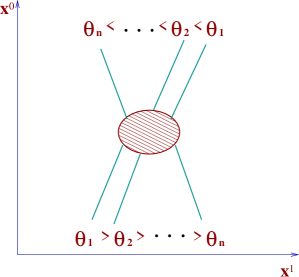
Figure 2.1: ${n}$-particle scattering process.

2.2.2 Higher spin conserved charges

Within the study of any QFT we will encounter in general two types of conserved charges. First of all, the familiar momentum and charges associated to internal symmetries of the model, which under the Lorentz group transform as vectors and scalars, respectively. Second, we can encounter also higher spin conserved charges namely, objects whose Lorentz transformations read

$$Q_{\ell}\rightarrow\Lambda^{\ell}Q_{\ell},$$ (2.66)

for $\Lambda$ a Lorentz boost. In particular, for $\ell=\pm 1$ we obtain the transformation laws of the light-cone components $p^{\pm}=p^{0}\pm p^{1}$ of the momentum ${p}^{\mu}=(p^{0},p^{1})$.

In what follows we shall make the assumption that the charges $Q_{\ell}$ are local, meaning that they can be expressed as integrals of local current densities

$$Q_{\ell}\sim\int\limits_{-\infty}^{\infty}d^{2}x\mathcal{T}_{\ell+1},$$ (2.67)

where $\mathcal{T}_{\ell+1}$ may be one of the integrals of motion defined in the previous section, which remains conserved in the perturbed CFT. However, one should keep in mind that also non-local conserved quantities can be present in the QFT at hand. Examples of such a situation have been studied in [84].

Provided (2.67) holds, the quantities (2.66) satisfy the following algebra of commutators

$$\left[Q_{\ell},Q_{n}\right]=0,$$ (2.68)

for all $n,\ell$. Since the light-cone components of the momenta and the masses of the particles are respectively conserved charges of spins 1 and 0, Eq. (2.68) indicates that the eigenstates of higher spin conserved quantities are linear combinations of eigenstates of the mass namely, states representing particles in the same mass multiplet. Consequently, each multiplet will contain a set of one-particle states which simultaneously diagonalise the momentum and charges $Q_{\ell}$, $\ell=\pm 1,\pm 2,..$. These states will be characterised as mentioned in the previous subsection by the vertex operators, $|V_{A}(\theta_{A})\rangle$ for $A$ to be the quantum numbers of the particle under consideration.

The eigenvalues of the charges $Q_{\ell}$ are determined by Lorentz invariance to be

$$Q_{\ell}|V_{A}(\theta_{A})\rangle=\xi_{A}^{\ell}(M_{A}e^{\theta_{A}})^{\ell}|V_{A}(\theta_{A})\rangle,$$ (2.69)

where $\xi_{A}^{\ell}$ are non-vanishing Lorentz scalars. The locality assumption (2.67) ensures that the generalisation of Eq. (2.69) to multi-particle states $|\theta_{1}\theta_{2}\cdots\theta_{n}\rangle$ is easily obtained as the sum of the actions over each individual particle state $|\theta_{A}\rangle$, $A=1,\cdots,n$,

$$Q_{\ell}|V_{A_{1}}(\theta_{1})V_{A_{2}}(\theta_{2})\cdots V_{A_{n}}(\theta_{n})\rangle=\left[\sum_{i=1}^{n}\xi_{i}^{\ell}(M_{i}e^{\theta_{i}})^{\ell}\right]|V_{A_{1}}(\theta_{1})V_{A_{2}}(\theta_{2})\cdots V_{A_{n}}(\theta_{n})\rangle$$ (2.70)

Let us now consider a scattering process with $k$ particles in the $in$-state and $n$ particles in the $out$-state. The associated scattering amplitude will be

$$S_{A_{1}A_{2}\cdots A_{k}}^{B_{1}B_{2}\cdots B_{n}}:=\langle V_{B_{1}}(\theta_{1})V_{B_{2}}(\theta_{2})\cdots V_{B_{n}}(\theta_{n})|V_{A_{1}}(\theta_{1})V_{A_{2}}(\theta_{2})\cdots V_{A_{k}}(\theta_{k})\rangle$$ (2.71)

where the S-matrix establishes a correspondence between the basis of $in$- and $out$-states. By looking at this completely general scattering process we can easily prove property ii) in the introduction, i.e. the absence of particle production or the fact that necessarily $n=k$ in (2.71). If $Q_{\ell}$ is a higher spin conserved quantity satisfying (2.70) it must remain conserved in the scattering process (2.71), namely

$$\sum_{i=1}^{k}\xi_{A_{i}}^{\ell}(M_{A_{i}}e^{\theta_{A_{i}}})^{\ell}=\sum_{i=1}^{n}\xi_{B_{i}}^{\ell}(M_{B_{i}}e^{\theta_{B_{i}}})^{\ell}.$$ (2.72)

If we further assume that the number of conserved charges $Q_{\ell}$ is infinite, the latter equation is really a system of infinitely many equations for different values of $\ell$ which, for generic values of the rapidities of the particles, admits only the trivial solution $n=k$ and

$$\theta_{A_{i}}=\theta_{B_{i}},\,\,\,\,\,\,\,\,\,\,\,\,\,\,\,\,\,\,\,\,\xi_{A_{i}}^{\ell}(M_{A_{i}})^{\ell}=\xi_{B_{i}}^{\ell}(M_{B_{i}})^{\ell},$$ (2.73)

for $i=1,\cdots,n$. Therefore, there is no particle production and the set of momenta of the particles in the $in$- and $out$-states must be the same. The only freedom allowed by the second set of equations in (2.73) is the possible exchange of quantum numbers between particles in the $in$- and $out$-state, in case there are more than one particle in each particle multiplet namely, the spectrum is degenerate.

The argument reported above can be found in [8, 81] and, as we have specified, requires the assumption of the existence of infinitely many conserved charges $Q_{\ell}$. This assumption allows also for proving the S-matrix factorisability, as we might see in the next subsection. However, it is interesting to report now the arguments exhibited by S. Parke in [10], who established quantum integrability as a consequence of the existence of only two of the mentioned conserved charges. These arguments can also be found in the review article [81]. In that case, the proofs of i),ii) are not so straightforward but due to the relevance of this result it is interesting to summarise here the key steps of Parke’s argument.

2.2.3 Factorisability and absence of particle production

The starting point of the argument in [10] and also of the proof of the S-matrix factorisability presented in [8] is the assumption that asymptotic one-particle states, $|\theta_{A}\rangle$ can be represented by means of localised wave packets $\Psi_{A}(x^{0},x^{1})$. Although the wave function formalism is not valid in the context of relativistic QFT, because of particle production and annihilation, we can make use of it when considering asymptotic multi-particle states ($in$- or $out$-states) namely, states describing a set of particles in the limits $t\rightarrow\pm\infty$, $t$ being the time, in which assuming a purely massive particle spectrum and short range interactions, particles become free. In that situation we can associate to each particle in the multi-particle $in$- ($|\theta_{A}\rangle$) or $out$-state ($\langle\theta_{A}|$), a localised wave packet

$$\Psi_{A}(x^{0},x^{1}) = \mathcal{N}\,\int{dp^{1}\,{e^{f(p^{1})}}}$$

$$f(p^{1}) = -a{(p^{1}-p^{1}_{A})}^{2}\,+\,i{(p^{1}(x^{1}-x^{1}_{A})-p^{0}_{A}(x^{0}-x^{0}_{A}))},$$ (2.74)

where $p^{1}_{A}$ is the mean spatial momentum of the particle $A$ and $p^{0}_{A}$ its energy. $\mathcal{N}$ is a normalisation constant and $(x^{0}_{A},x^{1}_{A})$ are the coordinates of the centre of the wave packet, namely the approximated time-space position of the particle $A$. Finally, the parameter $a$ is a constant expressing the spreading on the velocity of the wave packet. Therefore, any multi-particle state will be represented by a set of wave packets of this type whose overlapping regions are identified to be the regions where particles interact. The key property we want to use in the course of our argumentation is the fact that the transformation of the wave function (2.74) generated by an operator $e^{i\alpha Q_{\ell}}$, $\alpha$ being a free parameter, amounts to shifting the coordinates of the centre of the wave packet as follows

$$x^{0}_{A}\rightarrow x^{0}_{A}+\alpha\ell\xi_{A}^{\ell}(M_{A}e^{\theta_{A}})^{\ell-1},$$ (2.75)

$$x^{1}_{A}\rightarrow x^{1}_{A}+\alpha\ell\xi_{A}^{\ell}(M_{A}e^{\theta_{A}})^{\ell-1}.$$ (2.76)

A relevant characteristic is that the mentioned shift is not constant in general but, on the contrary, depends upon the rapidity of the particle under consideration. This is a crucial fact which means that when performing the same type of transformation for a multi-particle state, the outcome will be another multi-particle state where the mean positions of the particles differ from the original ones by a factor which is different for particles with different masses and rapidities. This observation turns out to be fundamental in order to prove the factorisability of the S-matrix into two-particle scattering matrices in massive 1+1-dimensional QFT’s.

Absence of particle production

The absence of particle production is a property which, as we have seen, is easily proven once the assumption of the existence of infinitely many higher spin conserved quantities is made. However, the proof becomes more involved if only two of these quantities are assumed to exist. We will not present here the details but only summarise the main ideas involved. First of all, the scattering amplitude must be invariant under transformations generated by the conserved charges $Q_{\ell}$ which means

$$S_{A_{1}A_{2}\cdots A_{k}}^{B_{1}B_{2}\cdots B_{n}}=e^{-i{\alpha}{Q_{\ell}}}S_{A_{1}A_{2}\cdots A_{k}}^{B_{1}B_{2}\cdots B_{n}}e^{i{\alpha}{Q_{\ell}}}.$$ (2.77)

In particular, Eq. (2.77) should also hold if we substitute $Q_{\ell}$ by a linear combination of two higher spin conserved quantities of spin $m$ and $-s$

$$Q_{\varphi}=\frac{\cos\varphi}{m}Q_{m}-\frac{\sin\varphi}{s}Q_{-s},$$ (2.78)

where $\varphi$ is a free parameter taking values in the interval $[0,2\pi)$. In [10] it was proven that any transformation generated by a conserved charge of type (2.78) acting on the scattering amplitude (2.77) for $k=2$ will lead to a violation of the macrocausality principle whenever the set of rapidities of the particles in the $in$- and $out$-states are different. The macrocausality principle states that the interaction time associated to the two incoming particles, say $t_{12}$, has to be always smaller of equal than the time at which any of the outgoing particles is produced. The key observation presented in [10] is that this principle could be violated if there was particle production in the scattering process and if the set of rapidities associated to incoming and outgoing particles are different. Consequently, the conclusion that $n$ should be always $2$ for the case at hand is immediate. Since in the next subsection we will see that any scattering amplitude can be ultimately expressed as a product of two-particle amplitudes, the proof of the absence of particle production can be easily generalised to any scattering process even when the number of incoming particles is bigger than two. In short, we can write

$$S_{A_{1}A_{2}\cdots A_{k}}^{B_{1}B_{2}\cdots B_{n}}\sim\delta_{kn}\prod_{i=1}^{n}\delta(\theta_{A_{i}B_{i}}).$$ (2.79)

Factorisability of the scattering amplitudes

The factorisability of any scattering amplitude in a 1+1-dimensional integrable QFT is easily proven provided a wave function description of the type (2.74) is used. As we have seen, the action of a conserved charge $Q_{\ell}$ on a multi-particle $in$- or $out$-state amounts to shifting the wave packet centres by a factor which is rapidity-dependent. The consequences of this property leading to the conclusion of the S-matrix factorisability are typically analysed by considering the three possible $3$   particle $\rightarrow$ $3$   particle scattering processes depicted in Fig. 2.2.

In a generic QFT there will not be in principle any reason to think the scattering amplitudes describing these three processes should have something to do with each other. However, if the theory possesses at least two higher spin conserved quantities, like the ones entering Eq. (2.78) and is 1+1-dimensional, the mentioned amplitudes are automatically forced to be identical. The reason is that any of the three diagrams in Fig. 2.2 can be transformed into each other by means of the ‘translation’ of one of the particles. Such a ‘translation’ can be generated by means of a conserved charge (2.78) and, according to (2.77), must leave invariant the corresponding scattering amplitude. Consequently, the processes in Fig. 2.2 correspond to the same scattering amplitude, which leads to the following set of equations

$$S_{A_{1}A_{2}}^{\,k\,\,p}(\theta_{12})S_{kA_{3}}^{B_{1}r}(\theta_{13})S_{\,p\,\,r}^{B_{2}B_{3}}(\theta_{23})=S_{A_{1}k}^{rB_{3}}(\theta_{13})S_{A_{2}A_{3}}^{\,p\,\,k}(\theta_{23})S_{\,r\,\,p}^{B_{1}B_{2}}(\theta_{12}).$$ (2.80)

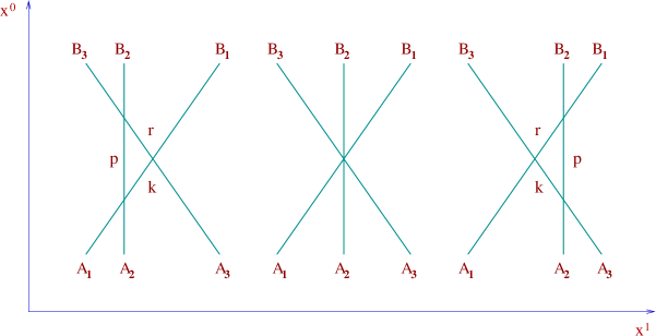
Figure 2.2: Graphical representation of the Yang-Baxter equation

It is also evident that the same argument holds for any $n\rightarrow n$ scattering process whose scattering matrix will then factorise into a product of $n(n-1)/2$ two-particle scattering amplitudes. Eq. (2.80) is known in the literature as Yang-Baxter equation [11]. In particular, when the number of particles in each particle multiplet is just one, i.e. the particle spectrum is non-degenerate, not only the rapidities but also the quantum numbers of the particles must be the same in the $in$- and $out$-states. In that case the S-matrix is diagonal, meaning that it has the general form

$$S_{A_{1}A_{2}}^{B_{1}B_{2}}(\theta_{12})=\delta_{A_{1}}^{B_{1}}\delta_{A_{2}}^{B_{2}}S_{A_{1}A_{2}}(\theta_{12}),$$ (2.81)

and consequently, the Yang-Baxter equation (2.80) becomes trivial. For this reason the construction of diagonal S-matrices is in general much simpler than in the non-diagonal case. In this thesis we will be concerned with the diagonal case, since the HSG S-matrices constructed in [51] are diagonal.

To close this section we would like to qualitatively show how the Coleman-Mandula theorem [5] turns out to be a very natural property in the light of the arguments of this section and, in particular, as a consequence of the properties of higher spin conserved quantities exploited here. Recall that the Coleman-Mandula theorem [5] states that, under certain assumptions, the S-matrix of any $1+d$-dimensional QFT with $d>1$ is trivial if the theory possesses any higher spin conserved quantity. The reason becomes clear if we consider any of the scattering processes in Fig. 2.2 but now in more than one space dimension. The existence of a single conserved charge $Q_{\ell}$ would allow us to ‘translate’ particles away from the plane where the interaction is taking place and to separate them from each other as much as we like. Therefore, the particles would not interact anymore and the scattering amplitudes should necessarily be trivial.

2.3 Analytical properties of two-particle scattering amplitudes

It is clear from the preceding section that the determination of the exact S-matrix associated to a 1+1-dimensional massive integrable model is equivalent to the exact computation of all two-particle scattering amplitudes, corresponding to the different $2\rightarrow 2$ scattering processes occurring in the theory. Therefore, before we enter the specific description of the non-abelian affine Toda field theories [47], it is interesting to provide a general description of the main properties of two-particle scattering amplitudes, paying special attention to non-parity invariant theories, since the S-matrices of the HSG-models which will enter our analysis in subsequent chapters break parity invariance. A more detailed derivation of these properties may be found in [12, 13, 14, 15, 16, 17].

In the context of 1+1-dimensional integrable QFT’s the calculation of exact two-particle S-matrices is possible by solving a set of constraining equations. These equations arise as a consequence of very general physical principles, in particular as we have stressed before, quantum integrability itself imposes severe restrictions on the two-particle scattering amplitudes which, in the non-diagonal case, must satisfy the highly non-trivial Yang-Baxter equation [11] reported in (2.80). Apart from the latter equation, the two-particle scattering amplitudes are constrained by other requirements which we itemise below

Lorentz invariance.

Analyticity.

Unitarity.

Crossing symmetry.

Moreover, in case bound states are present in the theory, the two-particle S-matrices have to obey the so-called bootstrap equations [12, 13] which we will report later. By solving the set of equations emerging from the previous constraints it is possible to determine the exact S-matrix of the theory up to certain multiplicative factors which, without adding any physical information, trivially satisfy all the constraining equations. These ambiguity factors are usually referred to as CDD-factors and their existence was pointed out in [19] by L. Castillejo, R.H. Dalitz and F.J. Dyson. They are usually fixed by appealing to consistency requirements, although these sort of arguments are in general not rigorous enough in order to make sure a certain S-matrix proposal is certainly correct, meaning it is really describing the scattering theory of a very specific model which is known through a Lagrangian formulation or by some other physical quantities. Recall that in the UV-limit one should recover the underlying CFT serving as starting point for our construction. For this reason it is desirable to develop tools which allow for consistency checks of the outlined proposal. The thermodynamic Bethe ansatz [20, 21] and form factor approach [22, 153] are precisely examples of this sort of tools which we might exploit in order to check the consistency of the S-matrix proposal [51] for the HSG-models.

Let us now commence with a more detailed discussion on the physical requirements summarised above. We already pointed out before that Lorentz invariance of the two-particle scattering amplitudes ensures that the S-matrix dependence upon the momenta of the particles has to enter via Lorentz invariant quantities. In particular, it is well known in 1+3-dimensions that the quantities we refer to are the so-called Mandelstam variables $s$, $t$ and $u$, defined as

$$s=({p}_{A}+{p}_{B})^{2},\,\,\,\,\,t=({p}_{A}-{p}_{C})^{2}\,\,\,\,\,u=({p}_{A}-{p}_{D})^{2},$$ (2.82)

for a scattering process of the type $A+B\rightarrow C+D$. However, in 1+1-dimensions only one of these three variables is really independent, so that the two-particle amplitudes shall depend only on one of Mandelstam’s variables, say $s$.

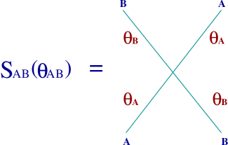
Figure 2.3: Two-particle scattering amplitude.

The sort of theories we will be interested in are characterised by a non-degenerate particle spectrum which ensures that the S-matrix will be diagonal, meaning that all two-particle scattering amplitudes have the form (2.81). Therefore, the Yang-Baxter equation (2.80) is trivially satisfied, in other words, it does not introduce any new constraint for the two-particle scattering amplitudes. Consequently, the incoming and outgoing particles involved in any two-particle scattering process have the same momenta (rapidities), say $p_{A},p_{B}$ ($\theta_{A},\theta_{B}$), in virtue of integrability, and the same quantum numbers, say $A,B$, due to the non-degeneracy of the spectrum (see Fig. 2.3). We will then denote such an amplitude by $S_{AB}(\theta_{AB})$. If the masses of the two incoming (outgoing) particles are $M_{A},M_{B}$, the Mandelstan variable $s$ reads

$$s=({p}_{A}+{p}_{B})^{2}=M_{A}^{2}+M_{B}^{2}+2M_{A}M_{B}\cosh\theta,$$ (2.83)

where, as usual $\theta=\theta_{AB}:=\theta_{A}-\theta_{B}$. The dependence of the $s$-variable on the rapidity difference is consequent with the discussion leading to Eq. (2.58).

We can now interpret the scattering amplitude $S_{AB}(\theta)=S_{AB}(s)$ as a function of the variables $s$ or $\theta$, which can take values in all the complex plane, namely we analytically continue the real variables $s$, $\theta$ to the complex plane. Once this is done, the unitarity and crossing symmetry of the scattering amplitudes, which we will talk about a bit later, imply that the amplitude $S_{AB}(s)$ must have square root branch points starting at the values $s=(M_{A}\pm M_{B})^{2}$ which correspond to $\theta=0,i\pi$ in the $\theta$-plane. These branch points give rise to branch cuts along the real axis $s\leq(M_{A}-M_{B})^{2}$ and $s\geq(M_{A}+M_{B})^{2}$ so that the two-particle amplitude, as a function of $s$, is not a meromorphic function. However, as a function of the $\theta$-variable, $S_{AB}(\theta)$ is a meromorphic function since, using the fact that $s(\theta)=s(-\theta)$, the mentioned branch cuts do not occur in the $\theta$-plane. In order to guarantee that the analytical continuation of the scattering amplitudes to the complex plane (both in $s$ and $\theta$) gives rise to uniquely defined functions, several Riemann sheets have to be considered. In particular, in the diagonal case, the number of Riemann sheets in the $\theta$-plane is just two. The physical values of the rapidity $\theta$ are constrained to the strip,

$$\text{Im}\,\theta\in(0,\pi).$$ (2.84)

The region of physical values of $\theta$ given in (2.84) is known under the name of physical sheet and corresponds to the first of the two Riemann sheets arising when diagonal scattering amplitudes are expressed in terms of the rapidity variable. Obviously, the relationship (2.83) between the $s$ and $\theta$ variables implies also that, associated to the region (2.84), there is a corresponding physical sheet for the $s$-variable.

As we shall see later in more detail, scattering amplitudes corresponding to the creation of stable bound states will be characterised by purely imaginary poles in the $\theta$-variable located at the physical strip, whereas the presence of unstable particles in the spectrum will be related to the existence of complex poles in the scattering amplitudes located in the second $\theta$ Riemann sheet, beyond the physical sheet (2.84).

Analyticity

Being the region of physical values of $s$ defined by (2.84), the physical values of the two-particle scattering amplitudes correspond to

$$S_{AB}^{\text{phys}}(s):=\lim_{\epsilon\rightarrow 0^{+}}S_{AB}(s+i\epsilon),$$ (2.85)

for $s$ to be real, in the spirit of Feynman’s $i\epsilon$ prescription in perturbation theory. Hermitian analyticity [85, 86, 87] then postulates that the physical scattering amplitude $S_{AB}(s)$ and its complex conjugated $[S_{BA}(s)]^{*}$ are boundary values in opposite sides of the $s$-plane branch cut of the same analytic function, namely

$$[S_{BA}^{\text{phys}}(s)]^{*}:=\lim_{\epsilon\rightarrow 0^{+}}S_{AB}(s-i\epsilon).$$ (2.86)

Taking furthermore into account that

$$\lim_{\epsilon\rightarrow 0^{+}}S_{AB}(s\pm i\epsilon)=S_{AB}(\pm\theta),\,\,\,\,\,\,\,\theta>0,$$ (2.87)

the Eqs. (2.85) and (2.86) translate into the condition

$$S_{AB}(\theta)=[S_{BA}(-\theta^{*})]^{*}$$ (2.88)

after analytic continuation to the complex plane and using the fact that if $S_{AB}(s)$ is an analytic function of $s$ the same holds for $[S_{AB}(s^{*})]^{*}$. A consequence of (2.88) is that the amplitudes $S_{AB}(\theta)$ will not be real analytic functions unless there are additional symmetries in the theory like parity invariance,

$$S_{AB}(\theta)=S_{BA}(\theta).$$ (2.89)

In that case the combination of (2.88) with the latter equation gives

$$S_{AB}(\theta)=[S_{AB}(-\theta^{*})]^{*},$$ (2.90)

which is the usual condition of real analyticity for two-particle scattering amplitudes. Therefore, the two-particle S-matrices are real analytic functions in 1+1-dimensional QFT’s only in the parity invariant case (for S to be diagonal). We will see later that some of the HSG S-matrices [51] provide particular examples of amplitudes which break parity invariance and therefore satisfy (2.88) instead of (2.90).

Unitarity

The S-matrix also has to be unitary, meaning that $SS^{\dagger}=1$ for physical values of the variables $s$, $\theta$. The unitarity of the S-matrix expresses the fact that the total probability of producing an arbitrary $out$-state from any initial $in$-state must be one. Physical unitarity together with the Hermitian analyticity condition (2.88) lead to

$$S_{AB}(\theta)S_{BA}(-\theta)=1,$$ (2.91)

which by analytic continuation to the complex plane can be assumed to hold for any complex value of $\theta$.

Crossing symmetry

The two-particle scattering amplitudes have to satisfy also the constraints derived from crossing symmetry which means they must remain invariant under the replacement of an incoming particle by an outgoing particle of opposite momentum. This leads to the constraint

$$S_{AB}(i\pi-\theta)=S_{B\bar{A}}(\theta),$$ (2.92)

where $\bar{A}$ denotes the antiparticle of the particle $A$. Notice that changing the momentum of the particle $A$ to $-p_{A}$ amounts to changing the Mandelstam $s$-variable to the $t$-variable, which explains the branch cut at $(M_{A}-M_{B})^{2}$. Eq. (2.92) expresses the fact that scattering processes described in the $s$- and $t$-channels are not independent from each other.

Bootstrap equations

All the constraints summarised above do not require any information about the particle content of the theory, they are completely general for any 1+1-dimensional integrable QFT and in fact, they are sufficient to establish already the general form of the two-particle scattering amplitudes, which in [88] were shown to be products of general building blocks depending upon hyperbolic functions of the form

$$f_{x}(\theta):=\frac{\sinh\frac{1}{2}\Big{(}\theta+i\pi x\Big{)}}{\sinh\frac{1}{2}\Big{(}\theta-i\pi x\Big{)}},$$ (2.93)

whenever the scattering matrix is assumed to be diagonal. The preceding building blocks (2.93) depend on certain variables $x$ which might encode the information about the particle spectrum of the theory. At this point, specific information about the QFT considered enters the S-matrix construction. It is clear that the block (2.93) has a simple pole corresponding to the value $\theta=i\pi x$. If the pole lies on the physical sheet $0<\text{Im}\,(\theta)<\pi$ which means $0<x<1$ it is assumed to be the trace of the formation of a stable bound state.

Let us now consider again the scattering amplitude $S_{AB}(\theta)$ which, in the light of the previous paragraph, will be a certain product of building blocks of the type (2.93). Suppose that, for the particular QFT at hand, the mentioned scattering amplitude possesses a simple pole $\theta=i\,u_{AB}^{C}$ characterising the formation of a stable bound state, say $C$, of mass $M_{C}$ in a scattering process of the type $A+B\rightarrow C$. By stable bound state we mean that particle $C$ is one of the asymptotic one-particle states present in the theory. Therefore, the mass of the bound state $C$ is given by,

$$M_{C}^{2}=M_{A}^{2}+M_{B}^{2}+2M_{A}M_{B}\cos u_{AB}^{C},$$ (2.94)

which is easily derived from (2.83) by considering the formation of particle $C$ in the centre-of-mass collision of particles $A,B$. Notice that Eq. (2.94) establishes a relationship between the masses of the stable particles present in the model. The values $u_{AB}^{C}$ are commonly referred to as fusing angles.

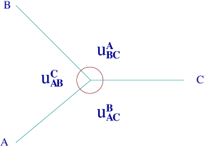
Figure 2.4: Fusing angles associated to the scattering processes ${A+B\rightarrow C}$, ${A+C\rightarrow B}$ and ${B+C\rightarrow A}$.

In fact, appealing to crossing symmetry, any of the three particles $A$, $B$ or $C$ may be seen as a bound state of the other two corresponding to fusing angles $u_{AB}^{C}$, $u_{BC}^{A}$ and $u_{AC}^{B}$ respectively. Consequently, we could write two more equations completely analogue to (2.94) by permuting the indices $A,B,C$. The combination of these equations leads to the constraint,

$$u_{AB}^{C}+u_{BC}^{A}+u_{AC}^{B}=2\pi,$$ (2.95)

which admits the graphic representation shown in Fig. 2.4.

The consideration of stable bound states as part of the asymptotic particle spectrum of the theory together with the integrability of the model leads to the so-called bootstrap equations [12, 13], which establish the equality of the scattering amplitudes related to the two scattering processes depicted in Fig. 2.5. Notice that again the representation of one-particle asymptotic states by means of localised wave packets together with Eqs. (2.75) and (2.76) are on the basis of the outlined relationship. Mathematically, this equivalence leads to the mentioned bootstrap equations which have the general form,

$$S_{AD}(\theta+i\bar{u}_{A\bar{C}}^{B})S_{BD}(\theta-i\bar{u}_{B\bar{C}}^{A})=S_{CD}(\theta),$$ (2.96)

where $\bar{u}_{AB}^{C}=\pi-u_{AB}^{C}$.

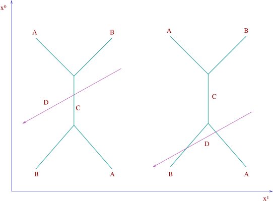
Figure 2.5: Graphical representation of bootstrap equations

Unstable particles

The discussion reported above refers exclusively to the presence of stable bound states related to purely imaginary simple poles in the rapidity variable located in the physical sheet, $0<\text{Im}\,(\theta)<\pi$. However, we might encounter a situation in which also unstable bound states can be present in the theory. In particular, the HSG-models on which we will mainly focus our attention later, provide examples of theories possessing unstable particles in their spectrum, that is, particles possessing a finite lifetime. Accordingly, some explanation is necessary concerning the interpretation of unstable bound states within the scattering theory context, in other words, we wish to identify the trace left by the formation of an unstable particle in a two-particle scattering amplitude.

Therefore, let us consider again a scattering process $A+B\rightarrow\tilde{C}$, where the particle $\tilde{C}$ is now unstable i.e., it is not encountered as part of the one-particle asymptotic spectrum which only contains particles whose lifetime is infinite. Similarly to the description of stable bound states, the unstable particle $\tilde{C}$ is expected to be produced whenever the particles $A$, $B$ scatter at a certain centre-of-mass energy $\sqrt{s}$ close enough to the mass of the unstable particle. In that case the scattering amplitude $S_{AB}(s)$ is expected to have a resonance pole located at a certain complex value of the Mandelstam variable $s$ given by

$$s_{R}:=M_{R}^{2}=\left[M_{\tilde{C}}-\frac{i\Gamma_{\tilde{C}}}{2}\right]^{2},$$ (2.97)

which shows that the description of unstable particles is usually carried out by complexifying the physical mass of a stable particle. In the $s$-plane, the mentioned complexification amounts to adding to the physical mass a complex contribution given by the decay width $\Gamma_{\tilde{C}}>0$, whose inverse is identified as the lifetime of the unstable particle. Therefore, the form of the two-particle S-matrix near to the resonance pole $s_{R}$ is given by the well known Breit-Wigner resonance formula [89, 14, 15]

$$S_{AB}(s)\approx 1-\frac{2iM_{\tilde{c}}\Gamma_{\tilde{C}}}{s-s_{R}}.$$ (2.98)

As mentioned in [14], whenever $M_{\tilde{C}}\gg\Gamma_{\tilde{C}}$ the following approximation

$$M_{R}^{2}\approx M_{\tilde{C}}^{2}+iM_{\tilde{C}}\Gamma_{\tilde{C}},$$ (2.99)

is justified, which allows for a clear-cut interpretation of $M_{\tilde{C}}$ as the physical mass of the unstable particle. The pole $s_{R}$ in the Mandelstam variable has a counterpart in the rapidity description which we will denote by

$$\theta_{R}=\sigma_{AB}^{\tilde{C}}-i\bar{\sigma}_{AB}^{\tilde{C}},$$ (2.100)

that is, in the $\theta$-plane, the presence of unstable particles in the models reflects in the existence of complex poles in the second Riemann sheet or non physical sheet. Therefore, $\sigma_{AB}^{\tilde{C}},\bar{\sigma}_{AB}^{\tilde{C}}>0$. In comparison to the description of stable particles, the fusing angles $u_{AB}^{C}$ describing stable bound states, get formally complexified as follows

$$u_{AB}^{C}\rightarrow-\bar{\sigma}_{AB}^{\tilde{C}}-i\sigma_{AB}^{\tilde{C}},$$ (2.101)

from where it is easily inferred that, unstable particles are associated to poles arising in the non physical sheet, namely $\textnormal{Im}(\theta_{R})$ is now negative. In addition, whenever the so-called resonance parameter $\sigma_{AB}^{\tilde{C}}$ is vanishing, the unstable particle $\tilde{C}$ becomes a ‘virtual state’, meaning that $\theta_{R}$ becomes purely imaginary as for the case of stable bound states, but still does not lie inside the physical strip. In that situation, unstable particles become virtual states characterised by poles on the imaginary axis beyond the physical sheet.

The particularisation of Eq. (2.94) to the case at hand amounts to substituting $M_{C}$ by $M_{R}$ and $u_{AB}^{C}$ as shown in (2.101). The identification of the real and imaginary part of this equation leads to the following relations

$$M_{\tilde{C}}^{2}-\frac{(\Gamma_{\tilde{C}})^{2}}{4} = (M_{A})^{2}+(M_{B})^{2}+2M_{A}M_{B}\cosh\sigma_{AB}^{\tilde{C}}\cos\bar{\sigma}_{AB}^{\tilde{C}},$$ (2.102)

$$M_{\tilde{C}}\Gamma_{\tilde{C}} = 2M_{A}M_{B}\sinh\sigma_{AB}^{\tilde{C}}\sin\bar{\sigma}_{AB}^{\tilde{C}}.$$ (2.103)

It becomes again clear from (2.102) and (2.103) that, whenever the resonance parameter $\sigma_{AB}^{\tilde{C}}$ is vanishing the unstable particle becomes a virtual state. The decay width $\Gamma_{\tilde{C}}$ vanishes in virtue of (2.103) as would correspond to an stable particle but, as mentioned above, the corresponding pole is located in the non physical sheet.

2.4 Non-abelian affine Toda field theories

In the preceding sections we have summarised the most relevant features of 1+1-dimensional integrable QFT’s. We started our study by reviewing their construction as perturbations of conformally invariant QFT’s and reported their most celebrated properties, which we have shown to be intimately linked to the powerful implications conformal symmetry has in 1+1-dimensions. As we have seen, the trace of these implications is still crucial once the CFT is driven away from its associated RG-fixed point. The most substantial consequence of the distinguished properties of 1+1-dimensional integrable massive QFT’s reported above is that, in many cases, they allow for the exact computation of the S-matrix of the theory under consideration. It is identified as the solution to a certain set of physically-motivated consistency equations expressing the requirements of unitarity, crossing symmetry, Hermitian analyticity and Lorentz invariance of the scattering amplitudes, together with the mentioned Yang-Baxter [11] and bootstrap equations [12, 13].

Having now settled the general framework and techniques, it is interesting to exploit these techniques in order to study a concrete family of 1+1-dimensional integrable theories, the so-called non-abelian affine Toda (NAAT) field theories [47], whose equations of motion were originally formulated by A.N. Leznov and M.V. Saveliev in 1983. The NAAT-theories are particular examples of Toda field theories which, as we have seen in the introduction, constitute field generalisations of the well known Toda lattice [32, 30, 31].

Clasically, the NAAT-equations [47] are integrable (multi-component) generalisations of the sine-Gordon equation for a bosonic field which takes values in a non-abelian Lie group, in contrast with the usual Toda field theories where the field takes values in the (abelian) Cartan subgroup of a Lie group [29]. The mentioned equations can be obtained as the equations of motion associated to an action functional which is the sum of the WZNW-action [57, 58, 78] associated to a complex non-abelian Lie group $\bar{G}_{0}$ and a bosonic field $h(x^{0},x^{1})$, and a potential $V(h)$, depending upon this field,

$$S[h]\>=\>{1\over\beta^{2}}\>\Bigl{\{}S_{WZNW}[h]\>-\>\int d^{2}x\>V(h)\Bigr{\}}\>.$$ (2.104)

Here $\beta$ is a coupling constant which does not play any role in the classical theory but gets quantized in the quantum theory in terms of an integer, $k$, usually referred to as “level” [57, 78, 3] (see also Eq. (2.125).

The latter structure already gives a first glimpse concerning the quantum formulation of these theories, which may be viewed, at least in some cases, as perturbations of a gauged WZNW-coset action [59, 60, 61, 64] by means of a primary field of the latter CFT. Consequently, all the properties and techniques described before in this chapter will inspire the quantum study of some NAAT-theories.

The most general construction of the NAAT-theories was carried out in [48] and takes as its starting point a semisimple, complex and finite Lie algebra denoted by $\bar{g}$, and a finite order automorphism $\sigma$ of the latter, which induces the following decomposition,

$$\bar{g} = \bigoplus_{\j\in\mathbb{Z}}\bar{g}_{\bar{\j}},\,\,\,\,\,\,\,\,\left[g_{\bar{\j}},g_{\bar{k}}\right]\subset\bar{g}_{\overline{\j+k}},$$ (2.105)

$$\sigma(x) = e^{2\pi ij/N}x,\,\,\,\,\,\,\,\,\text{for}\,\,\,\,\,\,\,x\in\bar{g}_{\bar{\j}}.$$ (2.106)

It is clear from (2.106) that $\sigma$ is an order-$N$ automorphism i.e., $\sigma^{N}=1$. A decomposition of the type (2.105) is referred to as a ${\mathbb{Z}}/{N\mathbb{Z}}$-gradation of the Lie algebra $\bar{g}$. The subindices $\bar{\j}$ must be understood as $\bar{\j}=\j\,\,\text{modulo}\,\,N$. Furthermore, the invariant subspace under the action of the automorphism, $\bar{g}_{0}$, is in virtue of (2.105), a complex subalgebra of $\bar{g}$, whose associated Lie group is denoted by $\bar{G}_{0}$. It is this Lie group where the field of every NAAT-theory related to a particular pair $(\bar{g},\sigma)$ takes values i.e., $h(x^{0},x^{1})\in\bar{G}_{0}$. Notice that until here we have always referred to finite Lie algebras, although the explicit construction of classically conserved charges requires the use of the affine or extended Lie algebra, $\hat{g}$.

Concerning the construction of quantum NAAT-theories, it was found in [48] (see also [90]) that, although there is a large class of interesting QFT’s related at classical level to NAAT-models, only a certain subset of NAAT-equations lead at quantum level to QFT’s possessing the following remarkable properties:

i) Unitarity, which in that context means we are interested in theories whose action functional takes real values. In other words, we wish to study the subset of theories which are expected to lead at quantum level to a Hilbert space containing only particle states of non-negative norm. In [48] it was shown that the reality condition is satisfied for the choice of action functionals whose kinetic term is positive-definite, whereas the potential is real and bounded from below.

ii) Existence of a mass-gap namely, we are interested in theories possessing a purely massive spectrum. Notice that our discussion of the preceding sections always referred to massive particles and accordingly, it is this sort of models which are expected to admit an S-matrix description of the type described in subsection 2.2.

In [48] the preceding requirements where shown to be only fulfilled by two families of NAAT-theories which were named as Homogeneous sine-Gordon (HSG) and Symmetric Space sine-Gordon (SSSG) theories and are in one-to-one correspondence with the different compact Lie groups and compact symmetric spaces, respectively. Actually, the HSG- and SSSG-theories of [48] are particular examples of the deformed coset models constructed by Q-H. Park in [63] and the Symmetric Space sine-Gordon models constructed by I. Bakas, Q-H. Park and H-J. Shin in [91], respectively, where the specific form of the potential makes them exhibit a mass gap namely, a purely massive particle spectrum.

Some remarks on classical integrability

The results presented in this thesis are mainly concerned with the quantum characteristics of the previously mentioned HSG- and SSSG-theories. For this reason, we want to report now in this subsection only a very briefly overview on the meaning and main implications of classical integrability, and its specific consequences in the context of NAAT-models. For a more detailed discussion concerning general aspects of classical integrability we refer the reader for instance to [92, 93]. The specific study of the classical integrability of the HSG- and SSSG-models was carried out in [49, 56] respectively, where the classically conserved charges were explicitly constructed.

The classical integrability of all NAAT-theories can be inferred from their associated equations of motion, which admit a zero-curvature expression of the form

$${\partial}_{-}(h^{-1}{\partial}_{+}h)=-m^{2}\left[\Lambda_{+},h^{-1}\Lambda_{-}h\right]$$ (2.107)

$$\Updownarrow$$

$$\left[{\partial}_{+}\,+h^{-1}{\partial}_{+}h+i\,m\Lambda_{+},{\partial}_{-}\,+i\,m\,h^{-1}\Lambda_{-}h\right]=0$$ ,

where we used the light-cone coordinates $x^{\pm}=x^{0}\pm x^{1}$. The objects $\Lambda_{\pm}$ are semisimple elements taking values in the subspaces $\bar{g}_{\bar{k}}$ and $\bar{g}_{\overline{N-k}}$ defined in (2.105) and (2.106) respectively. These elements enter into the expression of the potential $V(h)$ arising in (2.104) which has the general form

$$V(h)=-\frac{m^{2}}{\pi}\langle\Lambda_{+},h^{\dagger}\Lambda_{-}h\rangle,$$ (2.108)

where $m$ is a coupling constant that has mass dimension and the brackets $\langle\,,\,\rangle$ denote an invariant and non-degenerate bilinear form in $\bar{G}$ [94, 95].

The classical concept of integrability is encoded in Liouville’s theorem which defines a classically integrable model as a Hamiltonian system possessing at the same time a $2n$-dimensional phase space and $n$ independent conserved charges $Q_{i}$, $i=1,\cdots,n$ in involution, namely

$$\frac{\partial Q_{i}}{\partial x^{0}}=0,\,\,\,\,\,\,\,\,\,\,\,\,\,\,\,\{Q_{i},Q_{j}\}=0,\,\,\,\,\,\,\,\,\,\,i,j=1,\cdots,n,$$ (2.109)

$\{\,,\,\}$ denoting Poisson brackets.

As mentioned above, the zero-curvature expression (2.107) is intimately related to the classical integrability of NAAT-theories. This is based on the celebrated Lax-pair formalism commonly used in the formulation of classically integrable models. A Lax-pair $(L,B)$ is a pair of operators depending on the dynamical variables of the system at hand. Although the classical equations of motion of integrable systems are often non-linear, they can be formulated in terms of Lax-pairs in the form

$$\frac{\partial{L}}{\partial x^{0}}=\left[L,B\right].$$ (2.110)

Once a suitable Lax-pair $(L,B)$ has been constructed, the existence of infinitely many classically conserved charges follows immediately (see e.g. [92]) and their form is easily found to be $Q_{n}=\text{Tr}(L^{n})$. There are various ways to identify the most suitable Lax-pair associated to a certain model. In particular, the generalised Drinfel’d-Sokolov construction of [96] was used in [49, 56] to obtain the conserved densities related to (2.107) for the HSG- and part of the SSSG-models. It was also observed in [49, 56] that the classically conserved charges of a certain spin are recovered from the corresponding quantum higher rank conserved quantities in the limit $\hbar\rightarrow 0$. This result provides a consistency check for the quantum conserved charges constructed along the lines reported in subsection 2.1.2.

It is worth emphasising that one of the most important characteristics of classically integrable theories is the fact that their equations of motion very often posses solitonic and multi-solitonic solutions [93]. These sort of configurations turn out to be of special interest, since the classical interaction between solitons has, for classically integrable systems, very similar properties to the interaction of particles at quantum level, described by means of an S-matrix. The reason is that a soliton is defined as a non-singular solution to the classical non-linear equations of motion whose energy density is localised and remains undistorted under the time evolution. Consequently, soliton solutions have finite energy [93]. These properties suggest a relationship between soliton solutions and extended particles described by localised wave packets of the form (2.74). Indeed, very often at least part of the quantum spectrum of the model can be constructed by means of the semi-classical quantization of the classical solitonic solutions and there is a link between the semi-classical limit of the S-matrix and the solitonic solutions of the classical scattering [97, 93].

In particular, all NAAT-equations [47] admit solitonic solutions, which is in contrast with the usual affine Toda field theories [33, 34, 35, 36, 37], where the condition of having soliton solutions (imaginary coupling constant) leads to an ill defined action [98]. In particular in [50] the semi-classical spectrum of the HSG-models was constructed. Thereafter, the S-matrix proposal pointed out in [51] made use of this result by assuming the exact spectrum of stable particles at quantum level to coincide with part of the solitonic spectrum determined semi-classically. We will see in later chapters that all our consistency checks of the S-matrix proposal for the HSG-models have confirmed the legitimacy of the mentioned assumption.

Let us now turn to the description of some other general properties of NAAT-field theories and ultimately focus our attention in the homogeneous and symmetric space sine-Gordon models [48].

2.4.1 Quantum aspects of non-abelian affine Toda theories

Classically all NAAT-theories are integrable and make perfect sense for each possible choice of the objects $\{\bar{g},\sigma,\Lambda_{\pm}\}$ characterising their action functional (2.104). However, it was shown in [48] that not all classical NAAT-theories would be expected to lead at quantum level to well defined QFT’s in the sense described in the previous section (see i), ii)). It was found also in [48] that every consistent quantum NAAT-field theory will be described by an action of the form

$$S[h]\>=\>{1\over\beta^{2}}\>\Bigl{\{}S_{WZNW}[h]\>+\frac{m^{2}}{\pi}\>\int d^{2}x\>\langle\Lambda_{+},h^{\dagger}\Lambda_{-}h\rangle\Bigr{\}}\>,$$ (2.111)

where now the matrix element $\langle\Lambda_{+},h^{\dagger}\Lambda_{-}h\rangle$ entering the potential (2.108) is identified with a matrix element of a certain spinless primary WZNW-field i.e., at quantum level the potential $V(h)$ turns out to play the role of perturbing field in the sense of (2.39).

Therefore, the NAAT-theories will provide a Lagrangian formulation for some already known integrable perturbations of CFT’s and, furthermore, they will also lead us to discovering new ones.

The unitarity and the presence of a mass-gap in the theory are conditions which turn out to restrict severely the possible choices of the objects $\{\bar{g},\sigma,\Lambda_{\pm}\}$ at quantum level. In particular

i) The unitarity of the QFT requires an action functional whose kinetic term is positive-definite. This can only be achieved if the bilinear form $\langle\,,\,\rangle$ has a definite sign. This requires that the Lie group $G_{0}$ is chosen to be a compact Lie group. In that case the bilinear form $\langle\,,\,\rangle$ is the compact real form [94, 95]. This fact additionally implies, for $G_{0}$ to be non-abelian, that the field is unitary

$$h^{\dagger}=h^{-1}.$$ (2.112)

The latter property is only consistent with the NAAT-equations (2.107) if

$$\Lambda_{\pm}^{\dagger}=\Lambda_{\pm}\Rightarrow V(h)\in\mathbb{R}.$$ (2.113)

The previous equation, together with the conditions $\Lambda_{+}\in g_{k}$ and $\Lambda_{-}\in g_{N-k}$ reported in the previous section, restricts severely the possible inequivalent choices of the automorphism $\sigma$, which can only have order $N=1$ or 2. Then, the decomposition (2.105) gives

$$\sigma = 1\Rightarrow g=g_{0},\,\,\,\,\,\,\,\,\,\,\,\,\,\,\,\,\,\,\,\,\,\,\,\,\,\,\,\,\,\,\,\,\,\,\,\,\,\,\,\,\,\,\,\,\,\,\,\,\,\,\,\,\,\,\,\,\,\left[g_{0},g_{0}\right]\subset g_{0}$$ (2.114)

$$\sigma^{2} = 1\Rightarrow g=g_{0}\oplus g_{1},\,\,\,\,\,\,\,\,\,\,\left[g_{0},g_{1}\right]\subset g_{1},\,\,\,\left[g_{1},g_{1}\right]\subset g_{0},\,\,\,\left[g_{0},g_{0}\right]\subset g_{0}.$$ (2.115)

Accordingly,

$$\Lambda_{\pm}\in g_{0}\,\,\,\,\,\,\,\,\,\,\,\,\,\,\,\,\,\,\,\,\,\,\,\,\,\,\,\,\,\,\,\,\,\,\,\,\,\,\,\,\,\,\,\,\,\,\,\,\,\,\,\text{for $\sigma=1$},$$ (2.116)

$$\Lambda_{\pm}\in g_{1}\,\,\,\,\,\,\,\,\,\,\,\,\,\,\,\,\,\,\,\,\,\,\,\,\,\,\,\,\,\,\,\,\,\,\,\,\,\,\,\,\,\,\,\,\,\,\,\,\,\,\,{\text{for $\sigma^{2}=1$}}.$$ (2.117)

In this fashion we can restrict ourselves to the two families of NAAT-theories associated to the identity automorphism $(\sigma=1,N=1)$ or to involutions $(\sigma^{2}=1,N=2)$. The first family of theories are the already mentioned Homogeneous sine-Gordon models, whereas the NAAT- theories associated with involutions were named as Symmetric space sine-Gordon models [48], for the reason they are related to symmetric spaces in the way we will see later. However, at this stage of the construction there is still an additional requirement to be fulfilled.

ii) We wish to investigate theories with a purely massive particle spectrum. This leads to additional constraints which select out the precise CFT whose perturbations we want to investigate. The concrete details of the derivation of these constraints can be found in [48]. To put it briefly, the potential (2.108) can be shown to be globally invariant under certain transformations of the field

$$h(x^{0},x^{1})\rightarrow\alpha_{+}h(x^{0},x^{1})\alpha_{-},$$ (2.118)

for $\alpha_{\pm}\in g_{\pm}$ and $g_{\pm}$ being subalgebras of $g$. The breaking of such a symmetry amounts to the possibility of the existence of massless particles in the spectrum. In order to avoid that situation i.e., the degeneracy of the vacuum configuration, it is necessary to identify the mentioned symmetry with a gauge symmetry of the model, so that the different vacuum configurations are identified under gauge transformations. Therefore, one must substitute the classical action (2.104) by a gauged action for which is needed to modify the original WZNW-action associated to the Lie group $G_{0}$ by introducing certain gauge fields and select thereafter a particular gauge-fixing prescription. The outcome of the whole procedure is that the term $S_{WZNW}$ entering the action of the massive HSG- and SSSG-models (2.111) is a gauged WZNW-coset action [59, 60, 61, 64] associated to cosets of the general form $G_{0}/U(1)^{p}$ where $g_{\pm}=u(1)^{p}$ is the gauge symmetry algebra where the gauge fields take values, and

$$\,\,\,\,\,\,\,\,p=\ell,\,\,\,\,\,\,\,\,\,\,\,\,\,\,\,\,\,\,\,\,\,\,\,\,\Lambda_{\pm}\in U(1)^{\ell}\,\,\,\,\,\,\,\,\, \text{for the HSG-models},$$ (2.119)

$$0\leq\ell-\ell_{G/G_{0}}\leq p\leq{\mathrm{m}in\/}[\ell_{0},\ell-\nu],\,\,\,\,\,\,\,\,$$ for the SSSG-models (2.120)

Here $\ell,\ell_{0}$ are the ranks of the compact Lie algebras $g$ and $g_{0}$ respectively, $\ell_{G/G_{0}}$ is the rank of the compact symmetric space $G/G_{0}$, defined as the dimension of the maximal abelian subspaces contained in $g_{1}$ [66], and $\nu=2$ or 1 depending on whether $\Lambda_{+}$ and $\Lambda_{-}$ are linearly independent or not, respectively. In particular, the lower bound is reached when $\Lambda_{+},\Lambda_{-}\in g_{1}$ are regular, meaning that, the subset of elements of $g$ which simultaneously commute with $\Lambda_{\pm}$ constitute already a maximal abelian subspace of $g$. It is important to mention also here that, once the gauge has been fixed, the action (2.111) still possesses a remaining $U(1)^{p}$ global symmetry. This symmetry is responsible for the fact that the soliton solutions we will describe in the next subsection carry conserved Noether charges.

It is worth emphasising that the particular form of the abelian gauge transformation (2.118) has a crucial consequence which effects further results concerning the properties of the HSG S-matrices. The HSG- and SSSG-models are not parity invariant in general, unless the elements $\Lambda_{\pm}$ are not linearly independent from each other, namely $\Lambda_{+}=\eta\Lambda_{-}$. This is in the origin of the parity breaking of some of the scattering amplitudes we will encounter in the study of the HSG-theories.

iii) Moreover, if the quantum theory is to be well defined, the coupling constant has to be quantized: $\beta^{2}=1/k$, for some positive integer $k$ (see [57, 78, 56] for a more precise form of this quantization rule). Such a quantization does not occur in the sine-Gordon theory or the usual affine Toda theories because the field takes values in an abelian group in those cases. An important consequence of this is that, in the quantum theory, the $\beta^{2}$ will not be a continuous coupling constant. However, the quantum theory will have other continuous coupling constants that appear in the potential and, in particular, determine the mass spectrum.

The constraints stated in i),ii), iii) result in a rich variety of HSG- and SSSG-models. In summary:

I. The HSG-theories are perturbations of WZNW-coset theories associated to cosets of the type $G_{k}/U(1)^{\ell}$, for $\ell$ to be the rank of the compact Lie algebra $g$ and $k$ an integer which is identified with the level of the Kac-Moody representation of the Virasoro algebra [57] generating the conformal symmetry of the WZNW-models. These sort of CFT’s are also named as $G$-parafermion theories and their properties have been studied in [59, 60, 61].

II. The SSSG-theories include a larger variety of models, since the value of $p$ given by (2.120) is not fixed like for the HSG-models. They are associated to perturbations of WZNW-coset models related to cosets of the form $G_{0}/U(1)^{p}$. There are several interesting subclasses of SSSG-models that include, for $p=\ell_{0}$, new massive perturbations of the theory of $G_{0}$-parafermions different from those provided by the Homogeneous sine-Gordon theories [49]. Notice that this case happens only if the symmetric space satisfies $\ell_{0}\leq\ell-\nu$. Another particularly interesting class of models occurs when $\ell=\ell_{G/{G_{0}}}$ and $p=0$. In this case, the SSSG-theory is just a massive perturbation of the WZNW-model corresponding to $G_{0}$. We have named this particular subclass of theories as Split models and performed an investigation of their classical and quantum integrability in [56]. A scheme of some of the different types of Toda field theories, including the families of models studied here was presented in the previous chapter.

In the light of the preceding discussion, it is also clear that the HSG- and SSSG-models are just particular examples of NAAT-theories and it must be emphasised that they are not the only ones of physical interest. Other types of NAAT-theories have been also object of study in the literature (see for instance the work by J.F. Gomes et al. [99]).

Having now established the defining features of the families of models we will be interested in, we shall devote the next sections to a more detailed description of the properties of these theories which have been investigated in the literature. The study of the HSG-models has been carried out to a large extent over the last years. In [49] their classical integrability and quantum integrability were established. In [50] soliton and multi-soliton solutions were explicitly constructed by means of a semi-classical analysis. The latter semi-classical study has been also exploited in [51] for the explicit construction of all S-matrices describing the scattering theory of the HSG-models associated to simply-laced Lie algebras. On the other hand, the results available for the SSSG-theories are considerably more limited and the aim of this thesis has been also to partially fill this gap [56]. However, we will only report here the main conclusions of this work and focus more our discussion on the properties of the HSG-models to which we will continuously appeal in the next chapters.

2.4.2 The homogeneous sine-Gordon models

As we have explained in the previous paragraph there are many properties of the homogeneous sine-Gordon theories which are quite well understood for the time being and their quantum study has been carried out along the general lines described in sections 2.1, 2.2 and 2.3.

The simplest HSG-theory is associated to $G=SU(2)$, whose equation of motion is the complex sine-Gordon equation [62, 63]. This theory corresponds to the perturbation of the usual $\mathbb{Z}_{k}$-parafermions [64] by the first thermal operator [65], whose exact factorisable scattering matrix is the minimal one associated to $A_{k-1}$ [64, 33]. In fact, we will see later that the proposed scattering matrix [51] for the HSG-models related to simply laced Lie algebras consists partially of $\ell$ copies of minimal $A_{k-1}$-affine Toda field theory, whose mutual interaction is characterised by an S-matrix which violates parity.

The perturbing field characterising the action (2.111) was identified in [49] to be a spinless primary field having conformal dimension

$$\Delta=\bar{\Delta}=\frac{h^{\vee}}{k+h^{\vee}},$$ (2.121)

where $h^{\vee}$ is the dual Coxeter number of $g$. In the following we will often consider simply laced Lie algebras, so that we can write $h^{\vee}=h$ for $h$ to be the Coxeter number of $g$ whose definition may be found for instance in [100, 101, 78]. Combining (2.121) with the condition of super-renormalisability at first order (2.44), we obtain the constraint

$$k>h^{\vee}.$$ (2.122)

It is in this regime where the quantum integrability of the HSG-models has been established.

Furthermore, the remaining characteristics of the unperturbed CFT are well understood [59, 60, 78, 61] and in particular, one of the most relevant ones is, as usual, the associated central charge $c$,

$$c_{G_{k}/U(1)^{\ell}}=\frac{kh-h^{\vee}}{k+h^{\vee}}\,\ell.$$ (2.123)

Notice that (2.123) is nothing but the usual expression for the coset central charge [102] and we have used the general relation $\dim g=\ell(h+1)$.

Quantum integrability

The quantum integrability of the HSG-models was established by C.R. Fernández-Pousa, M.V. Gallas, T.J. Hollowood and J.L. Miramontes in [49] by means of the explicit construction of $\ell$ higher spin conserved densities, $\mathcal{T}_{s}$, of spin $s=\pm 2$ and $s=\pm 3$. In addition, classically conserved quantities associated to these same values of the spin were explicitly constructed by means of the mentioned generalised Drinfel’d-Sokolov construction [96]. Due to the specific choice of the objects $\{g,\sigma=I,\Lambda_{\pm}\}$ which characterise the HSG-models, it was shown that infinitely many classically conserved charges arise in these theories and that they are distributed in such a way that $\ell$ of them exist associated to each value of the spin $s=\pm 1,\pm 2,...$ At quantum level, this characteristic seems to be preserved, since the link between classical and quantum charges is achieved by identifying

$$J=J^{A}t^{A}=(\hbar k)\partial_{-}hh^{\dagger},\,\,\,\,\,\,\hbar k=\frac{1}{\beta^{2}}.$$ (2.124)

Here we explicitly introduced Plank’s constant in order to exhibit the precise relationship between the semi-classical, $\hbar\rightarrow 0$, the weak coupling, $\beta^{2}\rightarrow 0$, and the $k\rightarrow\infty$ limits. Notice that the second equality in (2.124) means that the semi-classical and weak coupling limits are equivalent. In Eq. (2.124) $J^{A}$ are the local currents which generate the conformal symmetry of the WZNW-model associated to the Lie algebra $g$, and $A=1,\cdots,\dim g$. The modes $J_{n}^{A}$ arising in the Laurent expansion of these currents satisfy a so-called Kac -Moody algebra

$$\left[J_{n}^{A},J_{m}^{B}\right]=f^{ABC}J_{n+m}^{C}+\frac{1}{2}k\,n\,\delta^{AB}\delta_{n+m,0},$$ (2.125)

which also provides a representation of the Virasoro algebra (2.12) by means of the so-called Sugawara construction [104]. The Kac-Moody algebra is characterised at quantum level, by a central extension given by the integer $k$ which is known as the level of the Kac-Moody representation [57, 78, 3] and takes always integer values. Finally the antihermitian generators $t^{A}$ arising in (2.124) provide a compact basis for the Lie algebra $g$ and their commutation relations $\left[t^{A},t^{B}\right]=f^{ABC}t^{C}$ involve the structure constants $f^{ABC}$ arising in (2.125).

The current $J$ and its anti-holomorphic counterpart are conserved in the original CFT,

$$\bar{\partial}{J(z)}=0,\,\,\,\,\,\,\,\,\,{\partial}{\bar{J}(\bar{z})}=0.$$ (2.126)

Since the holomorphic and anti-holomorphic components of the energy momentum tensor can be expressed in terms of the currents $J,\bar{J}$ by means of Sugawara’s construction [104] (see also [78, 3]), the previous equations imply the conservation of the energy momentum tensor in the unperturbed CFT.

As a consequence of the previous observations, the infinitely many locally conserved charges of the unperturbed CFT are generated by combinations of normal ordered products of the currents $J^{A},\bar{J}^{A}$, some of which remain conserved after the perturbation. Accordingly, the general form of the spin-2 and 3 conserved densities computed in [49] is

$$\mathcal{T}_{2}(z) = \mathcal{D}_{AB}(J^{A}J^{B})(z),$$ (2.127)

$$\mathcal{T}_{3}(z) = \mathcal{P}_{ABC}(J^{A}(J^{B}J^{C}))(z)+\mathcal{Q}_{AB}(J^{A}\partial J^{B})+\mathcal{R}_{A}(\partial^{2}J^{A})(z).$$ (2.128)

Here the parenthesis $(\,(\,\cdots\,)\,)$ denote normal ordering. The concrete normal ordering prescription for two arbitrary operators we are using here consists of selecting out the first regular term arising in their OPE. Such a prescription is used for instance in [103] and the second reference in [3].

Clearly, the latter densities are conserved in the original CFT in virtue of (2.126) and in [49] it was proven, by direct evaluation of Eq. (2.48), that, all the classically conserved spin-2 and 3 charges associated to the HSG-models give rise, at quantum level after a suitable renormalisation, to quantum conserved charges. These charges correspond to particular choices of the tensors $\mathcal{D}_{AB}$, $\mathcal{P}_{ABC}$, $\mathcal{Q}_{AB}$ and $\mathcal{R}_{A}$ in (2.127) and (2.128). Analogously, we may construct negative spin densities by changing $J\rightarrow\bar{J}$ in (2.127) and (2.128). Appealing now to the results reported in section 2.2, the existence of these conserved densities allows for concluding the quantum integrability of all HSG-theories. Recall that the counting argument has not been exploited for this class of theories for the reasons summarised at the end of subsection 2.1.2. Therefore, the HSG-models are expected to admit an S-matrix description and their exact S-matrix can be constructed by means of the bootstrap program [12] described in section 2.3.

The homogeneous sine-Gordon particle spectrum

The results of section 2.3 have shown that the exact S-matrices of 1+1-dimensional massive integrable QFT’s can be obtained as the solutions to a certain set of consistency equations expressing the physical requirements of analyticity, crossing symmetry, unitarity and Hermitian analyticity together with the Yang-Baxter and bootstrap equations, which are both highly non-trivial. The latter equations are the only ones which actually encode information concerning the specific nature of the theory under study. In particular, the bootstrap equations encode information about the pole structure of the S-matrix, intimately related to the presence in the model of stable and/or unstable particle bound states. The fusing angles $u_{AB}^{C}$ can be determined once the masses of the stable particles present in the theory are known by means of Eq. (2.94), which means the knowledge of the mass spectrum of the theory is fundamental in order to unravel the pole structure of the S-matrix.

Accordingly, we shall start our study by recalling the semi-classical mass spectrum associated to the HSG-models related to simply-laced Lie algebras, $g$, which was determined by C.R. Fernández-Pousa and J. L. Miramontes in [50]. In this paper the authors have shown that the equations of motion of the HSG-models (2.107) admit classical time-dependent soliton and multi-soliton solutions. Multi-soliton solutions associated to HSG-models related to simply-laced Lie algebras can be constructed by using the so-called solitonic specialisation, technique proposed by D.I. Olive et al. in [105] and linked thereafter to the method of dressing transformations in [106]. Furthermore, it was shown also in [50] that soliton and multi-soliton solutions associated to arbitrary HSG-theories can be constructed by using the well known soliton solutions arising in the complex sine-Gordon (CSG) model [65] and noticing that the latter model is nothing but the HSG-theory associated to $g=su(2)$. Thus, the construction of soliton solutions corresponding to arbitrary HSG-theories can be performed by embedding CSG one-soliton solutions into the $su(2)$ subalgebras of $g$ spanned by the Chevalley generators $\{E_{\pm\alpha},H_{\alpha}\}$ associated to each of its positive roots, $\alpha$ (see e.g. [94, 95, 101]).

When considered in their rest frame, the soliton solutions for the HSG-models are time-periodic and they allow for the investigation of the quantum spectrum of particles in the semi-classical approximation. This can be done by means of the so-called Bohr-Sommerfield quantization rule, which establishes that

$$S^{\text{sol}}+M^{\text{sol}}T^{\text{sol}}=2\pi n\hbar,\,\,\,\,\,\,\,n\in\mathbb{Z},$$ (2.129)

where $S^{\text{sol}}$, $M^{\text{sol}}$ and $T^{\text{sol}}$ are the action, mass and time-period of a classical soliton solution, respectively.

Proceeding this way, it was shown in [50] that, in the simply-laced case, there exist $k-1$ soliton solutions ($k$ being again the level) associated to each of the positive roots of $g$, whose masses are given by

$$M_{c}(\vec{\alpha})=\frac{k}{\pi}m(\vec{\alpha})\sin\Big{(}\frac{\pi c}{k}\Big{)},\,\,\,\,\,\,c=1,\cdots,k-1,$$ (2.130)

with

$$m(\vec{\alpha})=2m\sqrt{(\vec{\alpha}\cdot\Lambda_{+})(\vec{\alpha}\cdot\Lambda_{-})}.$$ (2.131)

The $m(\vec{\alpha})$ are the masses of the fundamental particles of the theory namely, the particles produced by fluctuations of the field $h$ around a vacuum configuration $h_{0}$. Their masses were identified by linearising the equations of motion in the approximation when the fluctuations are small ( i.e., $h=h_{0}e^{\varphi}$, $\varphi\ll 1$ ). As a consequence of the existence of a global symmetry associated to the Lie group ${U(1)}^{\ell}$ (see point ii) in the previous subsection), all soliton solutions of the theory carry a conserved Noether charge which was shown in [50] to have the form

$$Q_{c}(\vec{\alpha})=c\,\vec{\alpha}\,\,\text{modulo}\,\,k\Lambda_{R}^{*},\,\,\,\,\,\,\,\,\,c=1,\cdots,k-1,$$ (2.132)

where $\Lambda_{R}^{*}$ is the co-root lattice of $g$ [100, 95] which is the same as the root lattice in the simply-laced case, and $k$ is the level.

The result (2.130) shows that we can label each soliton solution, say $C$, by two quantum numbers $C:=(c,\vec{\alpha})$, notation which, with small modifications, turns out to be also natural for describing the quantum particle spectrum. It can be seen easily from (2.130) that whenever $c=a+b\,\,\text{modulo}\,\,k$ then

$$M_{c}(\vec{\alpha})<M_{a}(\vec{\alpha})+M_{b}(\vec{\alpha}),\,\,\,\,\,\,\,\,\,\,\,Q_{c}(\vec{\alpha})=Q_{a}(\vec{\alpha})+Q_{b}(\vec{\alpha}),$$ (2.133)

which supports the interpretation of the state $(c,\vec{\alpha})$ as a bound state of $(a,\vec{\alpha})$ and $(b,\vec{\alpha})$.

On the other hand, if we now consider the decomposition of any positive root $\vec{\alpha}$ in terms of simple roots $\vec{\alpha}_{1},\cdots,\vec{\alpha}_{\ell}$ of the Lie algebra $g$,

$$\vec{\alpha}=\sum_{i=1}^{\ell}{\kappa}_{i}\vec{\alpha}_{i},$$ (2.134)

we can see that

$$M_{c}(\vec{\alpha})\geq\sum_{i=1}^{\ell}M_{c\cdot{\kappa}_{i}}(\vec{\alpha}_{i}),\,\,\,\,\,\,\,\,\,\,\,Q_{c}(\vec{\alpha})=\sum_{i=1}^{\ell}Q_{c\cdot{\kappa}_{i}}(\vec{\alpha}_{i}).$$ (2.135)

Therefore, it is natural to expect the particle $(c,\vec{\alpha})$ to be unstable and decay into stable particles associated to the simple roots $\vec{\alpha}_{i}$, of the Lie algebra $g$.

Putting now together the results (2.133) and (2.135) we can already predict the stable and unstable bound state structure we might encounter at quantum level and, consequently, we have already an anticipation of the pole structure we expect to find when constructing the S-matrices associated to the HSG-models which enters the bootstrap equations (2.5). At this stage, we have the following picture concerning the quantum stable and unstable particle spectrum associated to the HSG-models (recall that we will focus our attention in the simply-laced case):

i) Associated to each simple root $\vec{\alpha_{i}}$, with $i=1,\cdots,\ell$, we have, according to (2.130), a tower of $k-1$ soliton solutions which may be associated to the stable particle spectrum at quantum level and whose masses will be assumed to be given by the same formula (2.130). We rewrite now this formula as

$$M_{a}^{i}:=M_{a}(\vec{\alpha}_{i})=\frac{k}{\pi}m_{i}\sin\Big{(}\frac{a\pi}{k}\Big{)},\,\,\,\,\,\,\,a=1,\cdots,k-1\,\,\,\,\,\text{and}\,\,\,\,\,i=1,\cdots,\ell.$$ (2.136)

Here we changed the notation for the masses of the fundamental particles in the obvious way $m(\vec{\alpha}_{i})=m_{i}$. Therefore, we expect to find $\ell\times(k-1)$ stable particles associated to each HSG-model corresponding to a coset of the form $G_{k}/U(1)^{\ell}$. The masses (2.136) coincide for each fixed simple root $\vec{\alpha}_{i}$ with the mass spectrum encountered for the minimal $A_{k-1}$-ATFT and, in fact, we may observe that the S-matrices describing the interaction of particles labeled by the same simple root will be the same found for the latter theories [33, 35, 36, 39, 107]. Accordingly, we may label the stable solitons (2.136) by two quantum numbers

$$A=(a,i),\,\,\,\,\,\,\,\,\,\,\,\,\,\,a=1,\cdots,k-1\,\,\,\,\,\,\,\,\,\,\,\,\,i=1,\cdots,\ell.$$ (2.137)

notation which we borrowed from [67], as we will see later. Due to the $\mathbb{Z}_{2}$-symmetry of the $A_{k-1}$-Dynking diagram each particle $A$ will have an associated antiparticle $\bar{A}$ of the same mass and quantum numbers $\bar{A}=(k-a,i)=\overline{(a,i)}$ similar to ATFT. The distinction between particles and anti-particles is possible in the HSG-models due to the existence of classically conserved charges associated to even values of the spin, which have opposite values for a particle and its anti-particle. Consequently, a particle and its associated anti-particles belong to different mass-multiplets, which turn out to be non-degenerate. For that reason the S-matrices determined by J.L. Miramontes and C.R. Fernández-Pousa in [51] are diagonal, as outlined before.

It is also interesting to present here the mass ratios $M_{c}^{i}/M_{c}^{j}$,

$$\frac{m_{i}}{m_{j}}=\frac{M_{c}^{i}}{M_{c}^{j}}=\sqrt{\frac{(\vec{\alpha}_{i}\cdot\Lambda_{+})(\vec{\alpha}_{i}\cdot\Lambda_{-})}{(\vec{\alpha}_{j}\cdot\Lambda_{-})(\vec{\alpha}_{j}\cdot\Lambda_{+})}}.$$ (2.138)

Since like in ATFT [35, 36, 39], the classical mass ratios are expected to remain preserved in the full quantum theory, this relation provides a direct link between full quantum and purely classical quantities.

ii) Additionally, every particle of mass (2.130) associated to a positive non-simple root, $\vec{\alpha}$, may be identified as an unstable particle and expected to decay into stable particles associated to the simple roots arising in the decomposition (2.134). In order to distinguish between stable and unstable particles we may use the same notation (2.137) for unstable particles but add to their quantum numbers a ‘tilde’. For instance, let us consider an unstable particle $\tilde{C}=(\tilde{c},\tilde{k})$ associated to a root $\vec{\alpha}$ which admits the decomposition $\vec{\alpha}=\vec{\alpha}_{i}+\vec{\alpha}_{j}$, in terms of simple roots. Then, one would expect to encounter a scattering process of the form

$$A+B\rightarrow \tilde{C} \rightarrow A+B,$$

$$\Updownarrow$$

$$(a,i)+(b,j)\rightarrow (\tilde{c},\tilde{k}) \rightarrow(a,i)+(b,j)$$ (2.139)

at quantum level. Following section 2.3, the presence of the unstable particle $(\tilde{c},\tilde{k})$ in the spectrum amounts to the existence of a corresponding resonance pole in the scattering amplitude $S_{AB}(\theta):=S_{ab}^{ij}(\theta)$ for a certain value of the rapidity $\theta_{R}=\sigma_{AB}-i\bar{\sigma}_{AB}$. Notice that, with respect to the general expression (2.100) in subsection 2.3, we have dropped out the upper index $\tilde{C}$ in $\sigma_{AB}$ and $\bar{\sigma}_{AB}$, which will simplify notations, without loss of information. In particular, for a scattering process like (2.139) we will denote the resonance parameter $\sigma_{AB}:=-\sigma_{ij}$ and the imaginary part of $\theta_{R}$, $\text{Im}(\theta_{R})=\bar{\sigma}_{AB}:=\bar{\sigma}_{ij}$. The scattering matrices associated to the formation of unstable particles have a novel feature in the HSG-models which distinguishes them from most of the diagonal scattering matrices associated to other 1+1-dimensional integrable massive QFT’s. This feature is the parity breaking $S_{AB}(\theta)\neq S_{BA}(\theta)$ whose origin is explained below.

In [50, 51] the following semi-classical relationship between the masses of the particles involved in the scattering process (2.139) whenever their quantum numbers satisfy $a=b=c=\tilde{c}$ was pointed out

$$(M_{\tilde{c}}^{\tilde{k}})^{2}=(M_{c}^{i})^{2}+(M_{c}^{j})^{2}+2M_{c}^{i}M_{c}^{j}\cosh\sigma_{ij}.$$ (2.140)

Here the definition (2.131) is crucial and the same relation (2.140) in fact holds for the corresponding fundamental particles. The parameters $\sigma_{ij}$ depend upon the roots and the elements $\Lambda_{\pm}$ as follows,

$$\sigma_{ij}=-\sigma_{ji}=\ln\,\sqrt{\frac{(\vec{\alpha}_{i}\cdot\Lambda_{+})(\vec{\alpha}_{j}\cdot\Lambda_{-})}{(\vec{\alpha}_{i}\cdot\Lambda_{-})(\vec{\alpha}_{j}\cdot\Lambda_{+})}}\,\,\,.$$ (2.141)

Since the HSG-theories are not parity invariant whenever the elements $\Lambda_{\pm}$ are linearly independent, we have to pay attention to the sign of the parameter $\sigma_{ij}$ in (2.140) which determines the sign of the rapidity difference $\theta_{c}^{i}-\theta_{c}^{j}:=\theta_{ij}$ of the incoming particles $(c,i),(c,j)$ at which the particle $(\tilde{c},\tilde{k})$ is produced. Remarkably, it was shown in [51] that only the positive sign i.e. $\sigma_{ij}>0$ is compatible with the classical integrability of the HSG-models related to simply-laced algebras. This conclusion was drawn on the basis of the explicit computation of the spin-$s$ classically conserved charges associated to the solitonic solutions constructed in [50] (see also the last reference in [47]). Notice that we have chosen the same name for the parameter $\sigma_{ij}$ as for the resonance parameter arising at quantum level when unstable particles are present in the theory. The reason is that these two parameters are indeed the same since the resonance poles of the S-matrix will be located at the values $\theta_{R}=-\sigma_{ij}-\frac{i\pi}{k}$. Therefore, in the semi-classical limit $k\rightarrow\infty$, $\theta_{R}\rightarrow-\sigma_{ij}$, which is fully consistent with (2.140).

The homogeneous sine-Gordon S-matrices

At this stage of the investigation the existence of a well-defined Lagrangian description for the HSG-models can give support to the conjecture that the formation of an unstable particle $(a,i)+(b,j)\rightarrow(\tilde{c},\tilde{k})$ really occurs at quantum level. It must be emphasised that, although other interesting 1+1-dimensional massive integrable theories whose S-matrices possess resonance poles have been investigated in the literature, they all lack a consistent Lagrangian description and have been formulated only from the point of view of scattering theory. Examples of this are the roaming trajectory or roaming sinh-Gordon models formulated by Al.B. Zamolodchikov in [108], their generalisations, due to M.J. Martins [109] and P. Dorey and F. Ravanini [110], and the theories possessing infinitely many resonance poles studied in [111].

The construction of the exact S-matrices associated to the HSG-models related to simply-laced Lie algebras carried out in [51] provides an interesting example of how the combination of various ingredients like, for instance, data extractable from different approaches, physically-motivated requirements or assumptions ultimately justified by the self-consistency of the results obtained, may lead to the exact calculation of two-particle scattering amplitudes within the context of 1+1-dimensional massive integrable models. Notice that, according to the results presented in section 2.3, the exact S-matrix associated to a 1+1-dimensional massive QFT whose mass spectrum is non-degenerate may always be expressed in terms of certain building blocks of the form (2.93), independently of the concrete theory under consideration. In the light of the results already presented in this section it is expected that the S-matrices of the HSG-models are diagonal. Thus, the really unknown data one needs to extract is the pole structure of the two-particle scattering amplitudes, which enters the building blocks (2.93) through the complex numbers $x$. As we also know, we expect to encounter two sorts of simple poles associated to real and complex values of $x$ in the physical strip. The techniques exploited in [51] in order to fix the positions of the latter poles can be summarised as follows:

i) Concerning the stable particle spectrum of the theory, in [51] the assumption that the soliton spectrum (2.136) computed semi-classically coincides with the exact mass spectrum of the stable particles encountered in the quantum theory has been fundamental. Once this assumption is made, the corresponding fusing angles associated to the formation of stable bound states are fixed by the equations (2.94). We already pointed out after Eq. (2.136) that the masses of the stable solitons coincide precisely with the mass spectrum arising in minimal $A_{k-1}$-ATFT [33]. In [51] it was found that, in fact, also the positions of the fusing angles computed through (2.94) are the same than in $A_{k-1}$-ATFT. Therefore, the natural conclusion is that the interaction between stable particles associated to the same simple root $\alpha_{i}$ is described by the two-particle scattering amplitudes $S_{ab}^{ii}(\theta)$ associated to minimal $A_{k-1}$-ATFT [33]. There are also other ways to determine these S-matrices like imposing $\mathbb{Z}_{k}$ invariance of the scattering amplitudes [33] or even using the knowledge of the values of the spin for which there are quantum conserved quantities in the theory. The mentioned S-matrices have the form,

$$S_{ab}^{ii}(\theta) = (a+b)_{\theta}\,(|a-b|)_{\theta}\prod_{n=1}^{\min(a,b)-1}(a+b-2n)_{\theta}^{2}\,\,$$ (2.142)

$$= \exp\int\frac{dt}{t}2\cosh\frac{\pi t}{k}\,\left(2\cosh\frac{\pi t}{k}-I\right)_{ab}^{-1}e^{-it\theta},$$ (2.143)

where the building blocks,

$$f_{x/k}(\theta):=(x)_{\theta}=\frac{\sinh\frac{1}{2}(\theta+i\frac{\pi x}{k})}{\sinh\frac{1}{2}(\theta-i\frac{\pi x}{k})}$$ (2.144)

have been used. Notice that Eq. (2.143) provides an integral representation for the scattering amplitudes which was derived in [68] and is part of the original results presented in this thesis. Such a representation is more convenient for the thermodynamic Bethe anstaz analysis we will carry out in the next chapter and also in the context of form factors, which will become clear in chapters 4 and 5. The calculation of (2.143) from the initial block expression (2.142) may be performed by specialising the analysis in [113, 41] to the particular case at hand (see also [42]). Although integral representations of scattering matrices appeared before in the literature (see e.g. [40, 42]), the analysis carried out in [41] goes further, providing a proof valid for all ATFT’s of the equivalence between such a representation and the usual representation in terms of hyperbolic functions employed in [51] for the original construction of the S-matrices of the HSG-models.

Notice the occurrence in (2.143) of the incidence matrix $I$, which is defined in terms of the Cartan matrix, $K$, as $I:=2-K$. The conclusion that the scattering amplitude (2.142) indeed describes the interaction between solitons labeled by the same simple root $\alpha_{i}$ was also checked for consistency by exploiting the knowledge of the HSG-Lagrangian, which allows for performing perturbation theory in the coupling constant, $\beta^{2}$. The key observation is that the results obtained from the tree-level calculation (see first reference in [35, 36]) of the scattering amplitude (2.142) must be recovered from the exact expression (2.142) upon the substitution $\beta^{2}=1/k$ and taking $k\rightarrow\infty$ thereafter, that is, in the semi-classical limit. This has been explicitly confirmed in [51].

ii) What is now left is the computation of the scattering amplitudes which involve the formation of unstable bound states. Having the Lagrangian (2.111) at hand one may perform perturbation theory in the coupling constant $\beta^{2}$ in order to determine the decay width associated to the process (2.139) together with the two-particle scattering amplitude in the tree-level approximation. The outcome of this calculation, whose details may be found in [51], allowed for checking that the process (2.139) corresponds in fact to the formation of an unstable bound state in the quantum theory and permitted the subsequent deduction of the position of the corresponding resonance poles arising in the scattering amplitudes $S_{ab}^{ij}(\theta)$. The latter result was obtained by using the fact that the general equation (2.102) for an unstable particle should reduce to Eq. (2.140) in the $k\simeq 1/\beta^{2}\rightarrow\infty$ limit and when considering a particle of very long lifetime, namely $\Gamma_{\tilde{c}}^{\tilde{k}}\ll M_{\tilde{c}}^{\tilde{k}}$. At the same time Eq. (2.103) must give in the same limit the decay width computed perturbatively. These constraints lead the authors of [51] to the following result,

$$S_{ab}^{ij}(\theta) = (\eta_{ij})^{ab}\prod\limits_{n=0}^{\min(a,b)-1}(-|a-b|-1-2n)_{\theta+\sigma_{ij}}\,,\quad\quad\quad K_{ij}^{g}\neq 0,2$$ (2.145)

$$= (\eta_{ij})^{ab}\exp-\int\frac{dt}{t}\,\left(2\cosh\frac{\pi t}{k}-I\right)_{ab}^{-1}e^{-it(\theta+\sigma_{ij})},\,\,\,K_{ij}^{g}\neq 0,2\,,$$ (2.146)

with $K^{g}$ denoting the Cartan matrix of the simply laced Lie algebra $g$. Here the $\eta_{ij}=\eta_{ji}^{*}$ are arbitrary $k$-th roots of $-1$ taken to the power $a$ times $b$ which have to be introduced in order to guarantee that the bootstrap equations (2.5) are fulfilled by these S-matrices. The shifts in the rapidity variables are functions of the vector couplings $\sigma_{ij}$ given by Eq. (2.141). Due to the fact that these shifts are real, the function $S_{ab}^{ij}(\theta)$ for $i\neq j$ will have poles beyond the imaginary axis at the positions

$$(\theta_{R})_{ij}=\sigma_{ji}-\frac{i\pi x}{k},$$ (2.147)

with $x=|a-b|+1+2n$ such that the parameters $\sigma_{ji}$ characterise resonance poles as we anticipated before. Therefore, the S-matrix (2.145) is not parity invariant and the parity breaking takes place through the phases $\eta_{ij}$ and the resonance parameters $\sigma_{ij}$. It can be proven that the latter amplitudes satisfy all the physical requirements presented in section 2.3. In particular, due to the parity breaking, the amplitudes (2.145) are not real analytic but satisfy the condition of Hermitian analyticity given by Eq. (2.88) [85, 86, 87]. The integral representation (2.146) was found in [68] in the context of the thermodynamic Bethe ansatz we will present in the next chapter.

iii) The remaining scattering amplitudes where shown to be $1$, namely particles associated to quantum numbers $(a,i)$, $(b,j)$, with $K_{ij}^{g}=0$ will interact freely.

In the light of (2.142) and (2.145) we can conclude that the proposed scattering matrix [51] for the HSG-models related to simply laced Lie algebras consists partially of $\ell$ copies of minimal $A_{k-1}$-ATFT [33], whose mutual interaction is characterised by the S-matrix (2.145), which violates parity.

How many free parameters do we have in our model?

The number of free parameters we have at our disposal will play a very important role in the course of the TBA- and form factor analysis since it determines the amount of plateaux we may observe when computing numerically the finite size scaling function and Zamolodchikov’s $c$-function [24]. For this reason, we want to devote a brief subsection to the computation of the amount of free parameters we expect to find in the HSG-models under consideration.

First of all, computing mass shifts from renormalisation, we only expect to accumulate contributions from intermediate states having the same colour as the two scattering solitons. Thus, making use of the well known fact that the masses of the minimal $A_{k-1}$-affine Toda theory all renormalise with an overall factor (see the first two references in [35, 36]), i.e. for the solitons $(a,i)$ we have that $\delta M_{a}^{i}/M_{a}^{i}$ equals a constant for fixed colour value $i$ and all possible values of the main quantum number $a$, we acquire in principle $\ell$ different mass scales $m_{1},\ldots,m_{\ell}$ in the HSG-models.

The previous argument is also in perfect agreement with the counting of free parameters which enter the S-matrix construction. As we have seen in detail before, we have $\ell$ different mass scales characterising the fundamental particles of the model (in one-to-one correspondence to the simple roots of $g$). In addition we find $\ell-1$ independent resonance parameters in the theory, $\sigma_{ij}=-\sigma_{ji}$ for each $i,j$ such that $K_{ij}^{g}\neq 0,2$, characterising resonance poles in the scattering amplitudes which are interpreted as the trace of the presence of unstable particles in the spectrum. Such an interpretation will be later confirmed by our TBA- and form factor analysis.

This means overall we have $2\ell-1$ independent parameters in the quantum theory. There is a precise correspondence to the free parameters which one obtains from the classical point of view. In the latter case we have the $2\ell$ independent components of $\Lambda_{\pm}$ at our free disposal. This number is reduced by $1$ as a result of the symmetry $\Lambda_{+}\rightarrow c\Lambda_{+}$ and $\Lambda_{-}\rightarrow c^{-1}\Lambda_{-}$ which introduces an additional dependence as may be seen from the explicit expressions for the classical mass ratios and the classical resonance shifts given by Eqs. (2.138) and (2.141). The masses of the stable particles of the model which will enter the TBA-equations (3.20) are given by Eq. (2.136).

As we have already said, the number of free parameters at our disposal, that is $2\ell-1$, will determine the maximum number of plateaux we may observe when computing the corresponding finite size scaling function. Such a result will also provide further support for the physical picture anticipated in [50, 51] for the HSG-models.

The exact computation of the S-matrix presented in this subsection closes our general review of the quantum properties of the HSG-models. As stressed before, one of the main results presented in this thesis is concerned with the development of consistency checks of the latter S-matrix proposal and also with a further development of the full QFT. The mentioned S-matrices are fully consistent at this point but their construction is based, as we have seen, on certain assumptions. Our consistency checks have been carried out within two different non-perturbative approaches known as thermodynamic Bethe ansatz [20, 21] and form factor approach [22, 153]. We will see in later chapters that all our results indeed confirm the consistency of the S-matrix proposal [51], meaning that all the relevant data characterising the underlying CFT which are extractable in those two approaches will be entirely consistent with our expectations based on the knowledge of the properties of the underlying coset CFT [59, 60, 61].

We will now describe the main results obtained for the other family of massive integrable non-abelian Toda field theories mentioned in this section, the SSSG-models. Some of the classical properties as well as quantum aspects of these theories have been studied in [56, 55] and we shall report very briefly in the next subsection our most prominent results. Although we will not go into detail about this second type of theories, it is mainly our intention to emphasise the richness of different massive non-abelian affine Toda field theories available. The latter statement should be clear in the light of Eqs. (2.119) and (2.120) and, in particular, the second of these equations shows that the SSSG-models represent a really huge class of theories whose quantum study has only been carried out to a very small extent in comparison to the HSG-theories described above. The interest of carrying out a more extensive study of these theories will be motivated below.

2.4.3 The symmetric space sine-Gordon models

In the same fashion the HSG-theories are in one-to-one correspondence with the finite, semisimple and compact Lie algebras, $g$, the classification of the SSSG-models exploits the existence of a correspondence between the SSSG-theories associated to a Lie algebra $g=g_{0}\oplus g_{1}$ and the compact symmetric spaces $G/G_{0}$, for $G$, $G_{0}$ to be the corresponding Lie groups associated to the Lie algebras $g,g_{0}$, which will be better justified later. The SSSG-models admit also a well-defined Lagrangian formulation (2.111), being now $h(x^{0},x^{1})$ a $G_{0}$-valued field. As we have also reported, these theories describe perturbations of either the WZNW CFT corresponding to $G_{0}$ or a coset CFT of the form $G_{0}/H$, where $H\simeq U(1)^{p}$ is a torus of $G_{0}$, not necessarily maximal. The equations of motion of this kind of theories for more general choices of the normal subgroup $H$ were originally considered in the context of the so-called reduced two-dimensional $\sigma$-models [114], although their Lagrangian formulation was not known until much later [91]. The results of [48, 90] show that they fit quite naturally into the class of non-abelian affine Toda theories and, what is more important, that the condition of having a mass gap requires that $H$ is either trivial or abelian. The simplest SSSG theories are the ubiquitous sine-Gordon field theory, which corresponds to $G/G_{0}=SU(2)/SO(2)$, and the complex sine-Gordon theory, which is related this time to $Sp(2)/U(2)$ [90] (recall that it is also the HSG theory associated to $SU(2)$). Actually, these two theories serve as paradigms of what can be expected in more complex situations. Other theories already discussed in the literature that belong to the class of SSSG theories are the integrable perturbations of the $SU(2)_{k}$ WZNW model and its $\widetilde{so(2)}$ reduction constructed by V.A. Brazhnikov [54]. Both of them are related to the symmetric space $SU(3)/SO(3)$ and, moreover, the second is identified with the perturbation of the usual $\mathbb{Z}_{k}$-parafermions by the second thermal operator.

The classification of the SSSG theories as perturbed CFT’s is achieved through the calculation of the central charge of the unperturbed CFT and the conformal dimension of the perturbation. Since the unperturbed CFT is always a coset CFT of the form $G_{0}/H$, its central charge is given by the usual expression (2.123) [102]. In contrast, the calculation of the conformal dimension of the perturbation requires the knowledge of the structure of the symmetric space.

A symmetric space $G/G_{0}$ is associated with a Lie algebra decomposition $g=g_{0}\oplus g_{1}$ that satisfies the commutation relations

$$[g_{0}\>,\>g_{0}]\subset g_{0}\>,\quad[g_{0}\>,\>g_{1}]\subset g_{1}\>,\quad[g_{1}\>,\>g_{1}]\subset g_{0}\>,$$ (2.148)

that is, precisely Eq. (2.115), which justifies in retrospect our statement concerning the correspondence between SSSG-theories and compact symmetric spaces. Then, the conformal properties of the perturbation depend on the structure of the representation of $g_{0}$ provided by $[g_{0},g_{1}]\subset g_{1}$. First of all, if the perturbation is to be given by a single primary field, then this representation has to be irreducible. This amounts to restrict the choice of $G/G_{0}$ to the so-called ‘irreducible symmetric spaces’ [66], which have been completely classified by Cartan and are labeled by type I and type II.

One of the most important results of our work [56, 55] has been the explicit computation of the conformal dimension of the perturbation corresponding to all the SSSG models related to type I symmetric spaces. This calculation can be done by making use of the relationship between the classification of type I symmetric spaces and the classification of the finite order automorphisms of complex Lie algebras and our results are reported in tables 2.1 and 2.2, for the cases when the Lie algebra, $g$, is classical and exceptional, respectively. It is worth noticing that this analysis only depends on the structure of the representation of $g_{0}$ given by $[g_{0},g_{1}]\subset g_{1}$. Therefore, our results apply to any SSSG related to a type I symmetric space, irrespectively of the choice of the normal subgroup $H$ that determines the coset $G_{0}/H$ and specifies the underlying CFT. For example, they provide the conformal dimension of the perturbation in the SSSG models constructed by I. Bakas, Q-H. Park and H-J. Shin in [91], which include the generalised sine-Gordon models related to the NAAT-equations based on $sl(2)$ embeddings constructed by T. Hollowood, J.L. Miramontes and Q-H. Park in [90]. It is also worth noticing that all the conformal dimensions reported tables 2.1, 2.2 decrease as $k$ increases, which means that $\Delta<1$ (the perturbation is relevant) above some minimal value of $k$ which is characteristic of each SSSG-theory. It is also clear that all the conformal dimensions obtained vanish in the semi-classical or weak coupling limit $k\rightarrow\infty$ which, according to Eq. (2.123) shows that the theory consists of $\dim g_{0}-p$ massive bosons in this limit.

In [56] it was also established the classical and quantum integrability of the subset of SSSG-theories which we named before as Split models. Recall that these models provide integrable perturbations of WZNW-models related to compact Lie groups $G_{0}$. It is expected that such integrability, which is ensured classically for all NAAT-theories in virtue of Eq. (2.107), extends to the quantum theory for all SSSG-models. Therefore, the latter family of models is expected to provide a huge class of new 1+1-dimensional integrable massive QFT’s which, in virtue of the general discussion of sections 2.1, 2.2 and 2.3, is by itself a motivation for their further study.

There are however various other reasons that justify the interest of a more extensive study of the quantum properties of the SSSG-theories:

i) First of all, although some already known integrable massive QFT’s are encountered as particular examples of SSSG-models, most of the SSSG-theories provide completely new perturbations of WZNW-coset theories (or of WZNW-theories for the case $p=0$ in Eq. (2.120)) which, in view of the results obtained in [49, 56], are expected to be quantum integrable. Therefore, all the study performed for the HSG-models could be generalised to the SSSG-theories and, in particular, they are expected to admit an S-matrix description at quantum level. In particular, in [56] part of the solitonic spectrum of the mentioned Split models was explicitly constructed. Also their classical and quantum integrability were established along the same lines as for the HSG-theories. In particular, the non-existence of classically conserved quantities which are associated to even values of the spin was shown . Recall that the existence of these charges allowed in [51] for the distinction between particles and anti-particles and was on the origin of the diagonal character of the S-matrix. Thus, as a novel feature, the S-matrices associated to the SSSG-models are expected to be in general non-diagonal, which will certainly make their construction more involved.

ii) The SSSG-models are expected to present the same type of distinguished features encountered for the HSG-models with respect to other integrable QFT’s. In particular, their S-matrices may break parity and have also resonance poles associated to unstable particles. The presence of unstable particles in the spectrum makes these theories capture realistic properties of QFT which are not often available in other bi-dimensional integrable models. Obviously, there is also a well-defined Lagrangian formulation for the SSSG-models. The parity breaking and presence of unstable particles in the spectrum have also specific consequences in the thermodynamic Bethe ansatz and form factor framework which further support the interest of these models. In particular, we expect to encounter the characteristic “staircase” pattern that we will find later for the scaling function of the HSG-models.

iii) Additionally, in [56] soliton solutions associated to a certain subset of the SSSG-models were found. For the models studied there these solutions have been shown to carry topological charges, similarly to the ones which characterise the sine-Gordon soliton and multi-soliton solutions (see for instance [93]). This in contrast to the soliton solutions constructed for the HSG-models [50], which carry Noether charges associated to the global $U(1)^{\ell}$ symmetry of the Lagrangian. However, for general SSSG-models, it was pointed out in [56] that, in fact, it is expected to encounter soliton solutions which may carry at the same time topological and Noether charges namely, “Dyon-like” solutions [115] to the classical equations of motion. To our knowledge, such feature has not been encountered before in the literature for other 1+1-dimensional massive integrable QFT and provides additional motivation for a further study of the SSSG-models.

2.4.4 The ${g|\tilde{g}}$-theories.

To close this chapter, we want to report some results concerning a family of theories recently proposed by A. Fring and C. Korff in [67] which contains the HSG-models and minimal ATFT’s as particular examples and can be understood, in fact, as a generalisation of them (see also [69, 71]). The particles arising in these models are labeled by two quantum numbers $(a,i)$, notation which we have borrowed in this thesis for labeling the HSG-solitons. Each of these quantum numbers is associated to a simply-laced Lie algebra in such a way that $a=1,\cdots,\ell$, for $\ell$ to be rank of a Lie algebra ${g}$ and $i=1,\cdots,\tilde{\ell}$, for $\tilde{\ell}$ to be the rank of a Lie algebra $\tilde{g}$. Consequently, the mentioned models have been named as $g|\tilde{g}$-theories. The corresponding two-particle scattering amplitudes will be denoted by $S_{ab}^{ij}$, notation which we have also used in this thesis for the HSG S-matrices and which slightly differs from the one used in the original literature [51]. The construction of the $g|\tilde{g}$-theories provided in [67] has been very recently generalised by C. Korff to the case when the $\tilde{g}$-algebra is non simply-laced [80].

The first quantum numbers $a,b$ govern the fusing structure and are usually referred to as main quantum numbers while the second quantum numbers $i,j$ will be named as colours and some of the scattering amplitudes corresponding to $i\neq j$ will break parity.

It is worth noticing that the construction of the $g|\tilde{g}$-theories carried out in [67] follows very different lines to what we have seen for the NAAT-models. The starting point in [67] is not the existence of a consistent Lagrangian formulation but a new S-matrix proposal which satisfies all the physical requirements presented in section 2.3 and therefore, is perfectly consistent form the scattering point of view. Consequently, a Lagrangian formulation is not known for the time being for a large subset of the $g|\tilde{g}$-theories, apart from the particular cases

$$A_{k-1}|\tilde{g}\equiv\,\,\,\,\, \tilde{G}_{k}\,\,\text{HSG-models},$$ (2.149)

$$g|A_{1}\equiv\,\,\,\,\,\,\,\,\,\, \text{minimal ATFT},$$ (2.150)

The S-matrix proposal presented in [67] takes advantage of the fact that for many theories the structure of the two-particle scattering amplitudes is of the form

$$S_{AB}(\theta)=S_{AB}^{\text{min}}(\theta)S_{AB}^{\text{CDD}}(\theta,B).$$ (2.151)

This is the case, for instance, for all ATFT’s related to simply-laced Lie algebras [35, 36] and also for the HSG-models. The first piece, $S_{AB}^{\text{min}}(\theta)$ is the so-called minimal S-matrix, which satisfies by itself all the physical requirements summarised in section 2.3. The second part, $S_{AB}^{\text{CDD}}(\theta,B)$, is a so-called CDD-factor [19], namely a function which satisfies trivially the conditions summarised in section 2.3 and at the same time does not have poles in the physical sheet. It depends on the effective coupling constant $B$.

The S-matrices characterising the $g|\tilde{g}$-theories were proposed in [67] to be,

$$S_{ab}^{ij}(\theta) = S_{ab}^{\text{min}}(\theta),\,\,\,\,\,\text{for $i=j$,}$$

$$S_{ab}^{ij}(\theta) = S_{ab}^{\text{CDD}}(\theta,B_{ij}),\,\,\,\,\,\,\text{for $i\neq j$}.$$ (2.152)

where as a novel feature the mentioned substructure $A=(a,i)$ for the particle quantum numbers was introduced. Accordingly, there are now a set of effective coupling constants $B_{ij}$ labeled by colour quantum numbers and satisfying $B_{ii}=0$. In [67] it was shown that the previous S-matrix proposal is perfectly consistent, meaning that, it satisfies all the necessary physical requirements. This is guaranteed by its definition (2.152), since both the minimal and CDD parts satisfy these requirements by themselves. Therefore every $g|\tilde{g}$-theory contains a set of $\ell\times\tilde{\ell}$ stable particles and is characterised by the existence of $\tilde{\ell}$ different mass scales. The corresponding S-matrix is given by (2.152) and its explicit form can be found in [67], where an integral representation, very useful in many contexts, was provided.

The thermodynamic Bethe ansatz (see chapter 3) carried out in [67] revealed that if as usual we view the $g|\tilde{g}$-theories as perturbed conformal field theories, the Virasoro central charge associated to the underlying CFT will have the general form

$$c_{g|\tilde{g}}=\frac{\ell\tilde{\ell}\tilde{h}}{h+\tilde{h}},$$ (2.153)

where $h,\tilde{h}$ are the Coxeter numbers of the Lie algebras $g,\tilde{g}$ respectively. The latter central charges coincide with the ones found in [61] for a class of parafermionic theories which can be interpreted as generalisations of the ones proposed in [59]. Also at the conformal level, when $g$ is taken to be not $A_{n}$, there exist so far no Lagrangian description.

$G/{G_{0}}$	$\ell_{G/G_{0}}$	$\Delta$
$SU(3)/SO(3)$	2	$\frac{6}{k+2}$
$SU(4)/SO(4)$	3	$\frac{4}{k+2}$
$SU(n)/{SO(n)}$,    $(n\geq 5)$	$n-1$	$\frac{n}{2(k+n-2)}$
$SU(2n)/Sp(n)$,    $(n\geq 1)$	$n-1$	$\frac{n}{k+n+1}$
${SO(n+2)}/{SO(n)\times U(1)}$,    $(n\geq 5)$	$2$	$\frac{n-1}{2(k+n-2)}+\frac{1}{2k}$
${SO(n+3)}/{SO(n)\times SO(3)}$,    $(n\geq 4)$	3	$\frac{n-1}{2(k+n-2)}+\frac{1}{k+2}$
${SO(n+m)}/{SO(n)\times SO(m)}$,    $(n,m\geq 4)$	min$(n,m)$	$\frac{n-1}{2(k+n-2)}+\frac{m-1}{2(k+m-2)}$
$Sp(n+m)/{Sp(n)\times Sp(m)}$,    $(n,m\geq 1)$	min$(n,m)$	$\frac{1+2n}{4(k+n+1)}+\frac{1+2m}{4(k+m+1)}$
${SU(n+m)}/{SU(n)\times SU(m)\times U(1)}$,	min$(n,m)$	$\frac{(n-1)(n+1)}{2n(k+n)}+\frac{(m-1)(m+1)}{2m(k+m)}+\frac{n+m}{2nmk}$
$(n,m\geq 2)$
${Sp(n)}/{SU(n)\times U(1)}$,    $(n\geq 2)$	n	$\frac{(n-1)(n+2)}{n(k+n)}+\frac{2}{nk}$
${SO(2n)}/{SU(n)\times U(1)}$,    $(n\geq 3)$	$[n/2]$	$\frac{n^{2}-n-4}{2n(k+n-1)}+\frac{2}{nk}$

Table 2.1: Conformal dimensions of the perturbations corresponding to the type I SSSG-models associated to the classical Lie groups $G$.

$G/{G_{0}}$	$\ell_{G/G_{0}}$	$\Delta$
${E_{6}}/{Sp(4)}$	6	$\frac{6}{k+5}$
${E_{6}}/{F_{4}}$	2	$\frac{6}{k+9}$
${E_{7}}/{SU(8)}$	7	$\frac{9}{k+8}$
${E_{8}}/{SO(16)}$	8	$\frac{15}{k+14}$
${F_{4}}/{SO(9)}$	1	$\frac{9}{2(k+4)}$
${E_{6}}/{SU(6)\times SU(2)}$	4	$\frac{21}{4(k+6)}+\frac{3}{4(k+2)}$
${E_{7}}/{SO(12)\times SU(2)}$	4	$\frac{33}{4(k+10)}+\frac{3}{4(k+2)}$
${E_{8}}/{E_{7}\times SU(2)}$	4	$\frac{57}{4(k+18)}+\frac{3}{4(k+2)}$
${F_{4}}/{Sp(3)\times SU(2)}$	4	$\frac{15}{4(k+4)}+\frac{3}{4(k+2)}$
${G_{2}}/{SU(2)\times SU(2)}$	2	$\frac{15}{4(3k+2)}+\frac{3}{4(k+2)}$
${E_{6}}/{SO(10)\times U(1)}$	2	$\frac{767}{128(k+8)}+\frac{1}{128k}$
${E_{7}}/{E_{6}\times U(1)}$	3	$\frac{527}{72(k+12)}+\frac{1}{72k}$

Table 2.2: Conformal dimensions of the perturbations corresponding to the type I SSSG-models associated to the exceptional Lie groups $G$.

Chapter 3 Thermodynamic Bethe Ansatz of the Homogeneous sine-Gordon models

The thermodynamic Bethe ansatz (TBA) is established as an important method which serves to investigate “off-shell” properties of 1+1 dimensional quantum field theories (QFT’s). Originally formulated in the context of the non-relativistic Bose gas by Yang and Yang [20], it was extended thereafter by Zamolodchikov [21] to relativistic quantum field theories whose scattering matrices factorise into two-particle ones. The latter property is always guaranteed when the QFT in question is integrable, as explained in the previous chapter. Provided the S-matrix has been determined in some way, for instance via the bootstrap program [12, 13] and/or by extrapolating semi-classical results as it is the case for the Homogeneous sine-Gordon (HSG) models, the TBA allows for calculating the ground state energy of the integrable model on an infinite cylinder whose circumference is identified as compactified time direction. When the circumference is sent to zero the effective central charge of the conformal field theory (CFT) governing the short distance behaviour can be extracted. In the case in which the massive integrable field theory is obtained from a conformal model by adding a perturbative term which breaks the conformal symmetry, the TBA constitutes an important consistency check for the S-matrix since it allows for the explicit computation of the Virasoro central charge associated to the underlying CFT.

The main purpose of this chapter is to apply this technique to the scattering matrices described in subsection 2.4.2 of the previous chapter, which have recently been proposed [51] to describe the HSG-models [48, 49, 50, 63, 90] related to simply laced Lie algebras. Within the TBA-context, we will investigate the physical picture anticipated for these models in the original literature i.e., we want to check for consistency the S-matrix proposal [51].

Although we have already summarised in the previous chapter the main features of the HSG-models, it is worth to emphasise again before entering our specific TBA-analysis, that the HSG-models possess very remarkable properties which distinguish them from many other 1+1-dimensional integrable quantum field theories studied in the literature so far, and that these properties have specific consequences in the TBA-analysis:

i) some of the two-particle S-matrices violate parity [51], namely $S_{AB}(\theta)\neq S_{BA}(\theta)$ in general. Such parity violation is intimately related in these theories to the existence of resonance poles in the S-matrix which, for the time being, we will assume are the only trace of the presence of unstable particles in the spectrum of a 1+1-dimensional integrable QFT. This feature i.e., the parity violation, will reflect itself in various ways along the TBA-analysis as, for instance, we may have to distinguish two sets of different TBA-equations (see section 3.2) or the so-called $L$-functions entering the TBA-analysis which are symmetric functions of the rapidity in parity invariant theories will not be symmetric anymore once any of the resonance parameters $\sigma_{ij}$ characterising the mass scale of the unstable particles is different from zero.

ii) the mentioned existence of unstable particles in the spectrum is also a remarkable feature by itself. Although the presence of resonance poles in the S-matrix has been observed also for other models like the roaming sinh-Gordon model originally introduced by Zamolodchikov in [108] and generalised thereafter in [109, 110], and also in [111, 112] where S-matrices containing an infinite number of resonance poles have been proposed, the HSG-models are distinguished essentially in two aspects. First, as we said, they break parity invariance and second, the HSG-models are not only consistent from the scattering theory point of view but also allow for a Lagrangian description [48] which makes possible the direct identification of some of the resonance poles with unstable particles [51] by means of a semi-classical analysis [50, 51]. However, the existence of resonance poles has similar effects in the outcome of the TBA-analysis for the HSG-models and for the models studied in [108, 109, 110]. In particular we shall observe that the finite size scaling function computed in the TBA turns out to have for the HSG-models a “staircase-like” behaviour, similar to the one originally observed for the roaming sinh-Gordon model [108] and for its generalisations [109, 110]. However, for the HSG-models such a behaviour admits a very nice physical interpretation when the resonance poles are understood as the trace of the presence of unstable particles in the spectrum. In this case the scaling function gives information about the energy scale at which the onset of every stable or unstable particle in the model takes place. This is a consequence of the fact pointed out in the previous chapter that the plateaux in the scaling function are directly related to the amount of free parameters in the model. Such a relationship does not hold neither for the roaming trajectory models [108], nor for the generalisations studied in [109, 110]. For these theories infinitely many plateaux arise in the scaling functions, although the amount of free parameters available is finite.

The main results presented in this chapter can be found in [68] (see also [69, 70, 71]). The chapter is organised as follows:

In section 3.1 we recall the basic ideas entering the thermodynamic Bethe ansatz approach [20, 21, 116]: in subsection 3.1.1 we start by studying a 1+1-dimensional integrable QFT in a circumference whose dimension $L$ will be sent to infinity in the so-called thermodynamic limit which we consider in subsection 3.1.2. The constraints for the momenta of the particles arising as a consequence of the introduction of periodic boundary conditions lead in the thermodynamic limit, when the equilibrium configuration is considered, to a set of coupled non-linear integral equations which are known as thermodynamic Bethe ansatz equations. They are presented also in subsection 3.1.2 for a general 1+1-dimensional integrable QFT. The study of the QFT in the thermodynamic limit at finite temperature is shown to be equivalent to its formulation on an infinite cylinder whose circumference is identified as the compactified time dimension. In the ultraviolet limit, we will derive a crucial relation between the equilibrium free energy of the QFT at finite temperature and the Virasoro central charge of the corresponding underlying CFT. The generalisation of this relationship from the critical point to the “off-critical” situation leads to the definition of the finite size scaling function as a measure of effective light degrees of freedom in a QFT and closes section 3.1. In section 3.2 we introduce the TBA equations for a parity violating system and carry out the ultraviolet limit recovering the expected coset central charge. We also justify and present in detail the approximations leading to the analytical calculation of the latter coset central charge. Section 3.3 is devoted to a detailed study of the TBA for the $SU(3)_{k}-$HSG model. In the subsequent subsections we discuss the “staircase” pattern of the scaling function and illustrate how the UV-limit for the HSG-model may be viewed as the UV-IR flow between different conformal models. We extract the ultraviolet central charges of the HSG-models. We study separately the case when parity is restored, derive universal TBA-equations and $Y$-systems. In section 3.4 we illustrate our analysis with several explicit examples which confirm the preceding analytical arguments. In particular the semi-classical limit $k\rightarrow\infty$ is studied in subsection 3.4.4. Finally, we state our conclusions and point out some open questions in section 3.5.

3.1 The thermodynamic Bethe ansatz approach

Before we attempt to carry out our specific TBA-analysis for the HSG-models we must introduce the basic ideas necessary for the understanding of the thermodynamic Bethe ansatz approach. The key points have already been anticipated very briefly in the introduction as well as the main motivation which justifies the interest of the TBA-approach in the context of 1+1-dimensional integrable quantum field theories. We may view a 1+1-dimensional massive integrable QFT as a certain integrable perturbation of a CFT by means of a relevant operator of the original or underlying CFT. Taking the original theory to be conformally invariant, there exists an infinite number of conserved quantities associated to it of which certain combinations might remain conserved in the perturbed QFT. For that reason, the perturbed QFT may be also integrable, namely, the corresponding S-matrix is factorisable in two-particle scattering matrices and there is no particle production in any scattering process. At this stage one might carry on and attempt to construct such S-matrix in the standard way i.e., by means of the bootstrap program [12, 13]. This procedure usually involves several assumptions. For example, for the models at hand, the HSG-models, the S-matrix proposal relies on the fundamental assumption that the soliton spectrum determined semi-classically coincides with the exact spectrum of stable particles at quantum level. This assumption is justified by the fact that the results obtained are self-consistent, namely the corresponding S-matrices [51] satisfy all the properties (2.88), (2.91), (2.92) and (2.96) introduced in the previous chapter and are consistent with the semi-classical physical picture [50, 51]. In addition, there exist usually some factors, the so-called CDD-factors originally introduced in [19], which one can always “add” to any S-matrix proposal, as they trivially satisfy all the requirements presented in section 2.3 and at the same time do not have poles in the physical sheet $0<\text{Im}(\theta)<\pi$. Therefore, provided we have been able to construct a S-matrix which is “candidate” for the description of the scattering theory associated to a very particular 1+1-dimensional integrable QFT, it is highly desirable to develop tools which permit to carry out this one-to-one correspondence. These consistency checks may consequently clarify finally the role of the mentioned ambiguities and assumptions. In this context, the thermodynamic Bethe ansatz approach turns out to be one of the tools we referred to above and so we intend to use it in order to check the consistency of the S-matrix proposal [51] for the HSG-models. Let us now review the basic ideas required in the thermodynamic Bethe ansatz approach, following the arguments presented in [21, 116, 117] (see also [37, 118, 69, 119]).

3.1.1 The Bethe wave function

Let us then start with a 1+1-dimensional integrable QFT whose S-matrix is factorisable and moreover diagonal, which will be the case for the HSG-models. Suppose also that we compactify the space dimension on a circumference of length $L$ which we assume to be very large since later we will consider the thermodynamic limit $L\rightarrow\infty$, $N_{A}\rightarrow\infty$, $N_{A}$ being the number of particles of type $A$, with $N_{A}/L$ finite. In general, a relativistic QFT can not be described by means of the wave function formalism. However, if we consider our system of $N=\sum_{A}N_{A}$ particles in the asymptotic limit in which all these particles are well separated from each other, meaning that their mutual interaction is negligible, we can associate to each of them a position $\{x_{1},\cdots,x_{N}\}$. In that situation, the system is describable in terms of a wave function $\Psi(x_{1},\cdots,x_{N})$ which is known as Bethe wave function and was originally proposed in [120].

Suppose now that we take one of these particles of type $A$, along the space direction, that is the circumference $[-L/2,L/2]$. Whenever there is another particle of type $B$ such that their positions $x_{A}$, $x_{B}$ are now close enough to allow a non-negligible interaction, the wave function description is not acceptable since the two particles can not be treated as free anymore. Clearly, their interaction will be characterised by the corresponding two-particle S-matrix $S_{AB}(\theta_{A}-\theta_{B})$. Therefore, the scattering theory must provide conditions in order to match the wave functions in the regions where the particle interactions are not negligible. Essentially, whenever the positions of two particles $A,B$ are interchanged, and interpreting then as $in$- and $out$-states, respectively, the wave function will pick up a factor $S_{AB}(\theta_{A}-\theta_{B})$. At the same time, since we have compactified the space dimension in the circumference $[-L/2,L/2]$ the wave function must also satisfy periodic boundary conditions,

$$\Psi(x_{1},\cdots,x_{A}=L/2,\cdots,x_{N})=\Psi(x_{1},\cdots,x_{A}=-L/2,\cdots,x_{N}).$$ (3.1)

Therefore, if we consider again a particle of type $A$ which is initially at the position $x_{A}=-L/2$ and we take it along the “world line” $[-L/2,L/2]$ so that it finally reaches the position $x_{A}=L/2$ the wave functions describing the initial and final situations should be identical since, taking (3.1) into account, there is not difference between the initial and final configurations. However, as we mentioned before, on its trip along the space direction the particle has interacted with all the other particles located at intermediate positions $-L/2<x_{i}<L/2$ and therefore the initial wave function must have picked up all the two-particle scattering amplitudes corresponding to each interaction. Consequently, by imposing the conditions,

$$\Psi(x_{1},\cdots,x_{A}=-L/2,\cdots,x_{N}) = e^{iLM_{A}\sinh\theta_{A}}\prod_{A\neq B}S_{AB}(\theta_{A}-\theta_{B})\times$$ (3.2)

$$\Psi(x_{1},\cdots,x_{A}=L/2,\cdots,x_{N}),$$

for $A=1,\cdots,n$, with $n$ being the number of particle species. Therefore, recalling now Eq. (3.1), we obtain the following set of constraints for the values of the rapidities $\theta_{A}$,

$$e^{iLM_{A}\sinh\theta_{A}}\prod_{A\neq B}S_{AB}(\theta_{A}-\theta_{B})=1\,\,\,\,\,\,\,\,\,\,\textnormal{for}\,\,\,\,\,\,\,\,\,\,A=1,\cdots,n.$$ (3.3)

Here $M_{A}$ is the mass of the particle species $A$ and, as usual, we write the momenta $p_{A}^{1}=M_{A}\sinh\theta_{A}$ in terms of the rapidities $\theta_{A}$. By taking now the logarithm of the latter equations and introducing the phase shifts

$$\delta_{AB}(\theta)=-i\ln S_{AB}(\theta),$$ (3.4)

we obtain a set of coupled transcendental equations for the rapidities

$$LM_{A}\sinh\theta_{A}+\sum_{B\neq A}\delta_{AB}(\theta_{A}-\theta_{B})=2\pi n_{A},\,\,\,\,\,\,\,\,\,\,\textnormal{for}\,\,\,\,\,\,\,\,\,\,A=1,\cdots,n,$$ (3.5)

which are known as Bethe ansatz equations. The numbers $n_{A}$ are integers which can be interpreted as quantum numbers labeling the multiparticle state at hand. In other words, the specific statistical nature of the particles enters through the collection of values $\{n_{1},\cdots,n_{n}\}$. Notice that in Eq. (3.5) we are associating one value $n_{A}$ to each particle species $A=1,\cdots,n$, therefore, each quantum number $n_{A}$ should be understood as a vector whose entries are the quantum numbers characterising each of the particles of the species $A$. For instance, if these particles are fermions, Pauli’s exclusion principle ensures that there can not exist two particles in the same quantum state, namely the values $(\theta_{A}^{(i)},n_{A}^{(i)})$ have to be different for each particle $i$. On the other hand, if the particles of a certain species $A$ are bosons, there is not a limit to the number of particles carrying the same quantum numbers. In addition, provided the $n_{A}$ entries are integers, the sum of all the equations (3.5) gives the expected quantization condition for the total momentum of a system

$$P=\sum_{A=1}^{n}M_{A}\sinh\theta_{A}=\frac{2\pi}{L}\hat{n}\,\,\,\,\,\,\,\,\,\,\textnormal{for}\,\,\,\,\,\,\,\,\,\,\hat{n}=\sum_{A=1}^{n}n_{A}\in\mathbb{Z},$$ (3.6)

subject to the periodic boundary conditions (3.1).

3.1.2 The thermodynamic limit

The Bethe ansatz equations (3.5) establish a set of constraints for the allowed rapidities of a system of $N$ particles subject to periodic boundary conditions. Let us now look at a particular particle species $A$ and suppose the system contains a number $N_{A}$ of particles of this type. As mentioned before, the corresponding quantum numbers $n_{A}$ occurring in Eq. (3.5) will have a certain substructure $\{n_{A}^{(1)},\cdots,n_{A}^{(N_{A})}\}$, namely the values $n_{A}^{(i)}$ must be interpreted as the individual quantum numbers of a particle $i$ of the species $A$. Similarly, we will denote the associated rapidities by $\theta_{A}^{(i)}$. Therefore, when solving the system (3.5) there will be solutions $\{\theta_{A}^{(i)}\}$ corresponding to the ‘allowed’ values of the quantum numbers $\{n_{A}^{(i)}\}$. These solutions are usually referred to as “roots”. Analogously, there will be a set of values of the rapidities $\{\theta_{A}^{(i)}\}$ which would be ‘solutions’ associated to the non permitted values of the quantum numbers $\{n_{A}^{(i)}\}$. These rapidities will be called “holes”.

The system (3.5) can be solved for the rapidities in the usual Bethe ansatz approach but in our case we will be interested in the so-called thermodynamic or low-density limit. In the thermodynamic limit both the dimension of the circumference $L$ where we compactified our system and the number of particles of each species $N_{A}$ are taken to be infinite whereas the density of particles of each type $N_{A}/L$ remains finite. In this macroscopic picture, it is useful to introduce three new functions which, following [21, 116, 117, 37, 118, 69, 119] we denote by $\rho^{(r)}_{A}(\theta)$, $\rho^{(h)}_{A}(\theta)$ and $\rho_{A}(\theta)$ and we define in the following way for each particle species $A$:

i) we define the function $\rho^{(r)}_{A}(\theta)$ as the rapidity density of “roots” per unit length, namely the number of particles of type $A$ possessing rapidities in an interval $[\theta,\theta+d\theta]$ divided by $L\,d\theta$,

$$\rho^{(r)}_{A}(\theta)=\frac{1}{L}\frac{dn_{A}^{(r)}}{d\theta},$$ (3.7)

where the superscript $r$ indicates that the integers $n_{A}^{(r)}$ are ‘allowed’ on the r.h.s. of (3.5), that is, they correspond to rapidities which are “roots” of (3.5).

ii) analogously , we can define now a function which measures the rapidity density of “holes” per unit length,

$$\rho^{(h)}_{A}(\theta)=\frac{1}{L}\frac{dn_{A}^{(h)}}{d\theta},$$ (3.8)

where the superscript $h$ in $n_{A}^{(h)}$ indicates that the corresponding rapidities $\theta_{A}$ are what we called “holes ”.

iii) Finally, we define the total rapidity density of states per unit length $\rho_{A}$ as

$$\rho_{A}(\theta)=\rho_{A}^{(r)}(\theta)+\rho_{A}^{(h)}(\theta)=\frac{1}{L}\frac{dn_{A}}{d\theta}.$$ (3.9)

In terms of the functions (3.7), (3.8) and (3.9), we can now safely carry out the thermodynamic limit ($L,N_{A}\rightarrow\infty$, $N_{A}/L$ finite) of (3.5). Hence, we obtain

$$\rho_{A}(\theta)=\rho_{A}^{(r)}(\theta)+\rho_{A}^{(h)}(\theta)=\frac{M_{A}}{2\pi}\cosh\theta+\sum_{B=1}^{n}\Phi_{AB}*\rho_{B}^{(r)}(\theta),$$ (3.10)

where the functions $\Phi_{AB}(\theta)$ containing the information about the dynamical interaction of the system are given, with the help of (3.4), by

$$\Phi_{AB}(\theta)=\Phi_{BA}(-\theta)\;=\frac{d\delta_{AB}(\theta)}{d\theta}=-i\frac{d}{d\theta}\ln S_{AB}(\theta)\,.$$ (3.11)

They are usually called kernels, and the symbol ‘  *  ’ denotes the rapidity convolution defined as

$$f*g(\theta):=\int\limits_{-\infty}^{\infty}\frac{d\theta^{\prime}}{2\pi}\,f(\theta-\theta^{\prime})g(\theta^{\prime}),$$ (3.12)

for two arbitrary functions $f$ and $g$. In (3.10) the densities of “roots” and “holes” $\rho_{A}^{(r)}$, $\rho_{A}^{(h)}$ are independent functions, which makes the system (3.10) still difficult to handle. However, additional constrains can be obtained when the equilibrium configuration at a certain finite temperature $T$ is studied. The thermodynamic equilibrium of the system is equivalent to the minimisation of the total free energy per unit length, which we denote by $f(\rho,\rho^{(r)})=\sum_{A}f(\rho_{A},\rho_{A}^{(r)})$ and is given by

$$f(\rho,\rho^{(r)})=h(\rho^{(r)})-Ts(\rho,\rho^{(r)}),$$ (3.13)

where the functions $h(\rho^{(r)})$ and $s(\rho,\rho^{(r)})$ are respectively the total energy and entropy of the system per unit length, i.e.,

$$h(\rho^{(r)}) = \sum_{A=1}^{n}h(\rho_{A}^{(r)})=\sum_{A=1}^{n}\int\limits_{-\infty}^{\infty}d\theta\,\rho_{A}^{(r)}(\theta)M_{A}\cosh\theta,$$ (3.14)

$$s(\rho,\rho^{(r)}) = \sum_{A=1}^{n}s(\rho_{A},\rho_{A}^{(r)})=\sum_{A=1}^{n}\ln{\mathcal{N}}(\rho_{A},\rho_{A}^{(r)}).$$ (3.15)

Here ${\mathcal{N}}(\rho_{A},\rho_{A}^{(r)})$ has to be understood as the density of quantum states labeled by the integers $n_{A}^{(i)}$ with $A=1,\cdots,n$ and $i=1,\cdots,N_{A}$, which correspond to the same density configuration $\rho_{A},\rho_{A}^{(r)}$. It can be computed as follows: Let $N^{\prime}_{A}$ be the number of quantum levels associated to the particle species $A$ contained in a rapidity interval $[\theta,\theta+d\theta]$. Taking definition (3.9) into account, it follows that $N^{\prime}_{A}\approx\rho_{A}(\theta)d\theta$. Let $n^{\prime}_{A}$ be the number of particles of type $A$ distributed in the same interval, namely $n^{\prime}_{A}\approx\rho_{A}^{(r)}(\theta)d\theta$. Taking Pauli’s exclusion principle into account one can easily obtain the number of different possible distributions of these $n^{\prime}_{A}$ particles of type $A$ between the $N^{\prime}_{A}$ different quantum levels,

$$\frac{N^{\prime}_{A}!}{n^{\prime}_{A}!(N^{\prime}_{A}-n^{\prime}_{A})!} \approx \frac{[\rho_{A}(\theta)d\theta]!}{[\rho_{A}^{(r)}(\theta)d\theta]![(\rho_{A}(\theta)-\rho_{A}^{(r)}(\theta))d\theta]!},\,\,\,\,\textnormal{fermionic case}$$

$$\frac{(N^{\prime}_{A}+n^{\prime}_{A}-1)!}{n^{\prime}_{A}!(N^{\prime}_{A}-1)!} \approx \frac{[(\rho_{A}(\theta)-\rho_{A}^{(r)}(\theta)-1)d\theta]!}{[\rho_{A}^{(r)}(\theta)d\theta]![(\rho_{A}(\theta)-1)d\theta]!},\,\,\,\,\,\,\,\,\textnormal{bosonic case}$$ (3.16)

Therefore, the corresponding entropies read

$$s(\rho,\rho^{(r)}) = \sum_{A=1}^{n}\int\limits_{-\infty}^{\infty}d\theta\Big{(}\rho_{A}\ln\rho_{A}-\rho_{A}^{(r)}\ln\rho_{A}^{(r)}-(\rho_{A}-\rho_{A}^{(r)})\ln(\rho_{A}-\rho_{A}^{(r)})\Big{)},\,\,\,$$ (3.17)

$$s(\rho,\rho^{(r)}) = \sum_{A=1}^{n}\int\limits_{-\infty}^{\infty}d\theta\Big{(}\rho_{A}\ln\rho_{A}-\rho_{A}^{(r)}\ln\rho_{A}^{(r)}-(\rho_{A}+\rho_{A}^{(r)})\ln(\rho_{A}+\rho_{A}^{(r)})\Big{)},\,\,\,$$ (3.18)

for the species $A$ to be fermions or bosons respectively. Notice that, in the derivation of the latter equations we have used Stirling’s formula $\ln N!\approx N(\ln N-1)\approx$$N\ln N$ for $N\gg 1$.

Having now explicit expressions for the energy and entropy of the system in terms of the densities $\rho_{A}$ and $\rho_{A}^{(r)}$ we are in the position to express the free energy per unit length (3.13) in terms of the mentioned densities and determine the extremum conditions corresponding to both fermionic and bosonic statistics. For this purpose it is convenient to define a set of new functions $\epsilon_{A}(\theta)$ which are referred to as “pseudo-energies” and which can be expressed in terms of the densities of “roots” and “holes” as follows,

$$e^{\epsilon_{A}} = \frac{\rho_{A}}{\rho_{A}^{(r)}}-1=\frac{\rho_{A}^{(h)}}{\rho_{A}^{(r)}},\,\,\,\,\,\,\textnormal{fermionic case},$$

$$e^{\epsilon_{A}} = \frac{\rho_{A}}{\rho_{A}^{(r)}}+1=\frac{\rho_{A}^{(h)}}{\rho_{A}^{(r)}}+2,\,\,\,\,\,\,\textnormal{bosonic case}.$$ (3.19)

Therefore, with the help of (3.10) and (3.11), the extremum conditions for the free energy per unit length (3.13) read,

$$\epsilon_{A}(\theta)=RM_{A}\cosh\theta-\sum_{B}\Phi_{AB}*L_{B}(\theta),$$ (3.20)

where $R=1/T$ and we have introduced the $L$-functions

$$L_{A}(\theta)=\ln(1+e^{-\epsilon_{A}(\theta)}),\,\,\,\,\,\,\,\,\,\,\,\,\,\,\,\,\textnormal{fermionic case},$$

$$L_{A}(\theta)=-\ln(1-e^{-\epsilon_{A}(\theta)}),\,\,\,\,\,\,\,\,\,\,\,\,\,\,\,\,\,\textnormal{bosonic case}.$$ (3.21)

From (3.20) and (3.21) one easily sees that whenever the S-matrix reduces to $\pm 1$, namely we study a system of free fermions or bosons, the pseudo-energies are simply given by

$$\epsilon_{A}(\theta)/R=M_{A}\cosh\theta,$$ (3.22)

that is, the free “on-shell” energies.

The non-linear integral equations (3.20) are usually called thermodynamic Bethe ansatz equations. In general, omitting the systems of free fermions or bosons studied in [116], the system (3.20) can not be solved analytically for the pseudo-energies for generic temperature, and we may ultimately resort to numerical methods. Once the pseudo-energies $\epsilon_{A}(\theta)$ have been computed in some way and, consequently the $L$-functions, it is possible to obtain the free energy of the system (3.13) subject to the extremum conditions (3.20) namely, the extremal free energy

$$f(R)=-\frac{1}{R}\sum_{A=1}^{n}M_{A}\int\limits_{-\infty}^{\infty}\frac{d\theta}{2\pi}L_{A}(\theta)\cosh\theta,$$ (3.23)

therefore, taking (3.22) into account, the equilibrium free energy for a system of free bosons or fermions reduces to the one of a relativistic Fermi or Bose gas at finite temperature $T=1/R$ (see section 6 in [116]).

As we will show later, the extremal free energy (3.23) is directly related to the ground state energy of the system which at the same time, in the UV limit, depends on the Virasoro central charge of the underlying CFT. These relationships justify the link between the infinite volume thermodynamics of a QFT, expressed in terms of its corresponding S-matrix by means of (3.20), and some of the relevant data characterising the original CFT.

Quantum field theory on a torus

As stated in several occasions, the analysis performed before is based on the study of a QFT compactified on a circumference of length $L$, which is taken to be infinity in the thermodynamic limit. Let us assume now that we formulate our QFT on a torus generated by two orthogonal circles of circumferences $R$ and $L$ and define a Cartesian (Euclidean) coordinates system in the way showed in Fig. 3.1. In that situation, we have at our disposal two possible choices for the quantization axis i.e., two possible ways to develop a quantum mechanical formulation of the theory, depending on whether we identify the directions $x$, $y$ with the space and time dimensions or vice-versa:

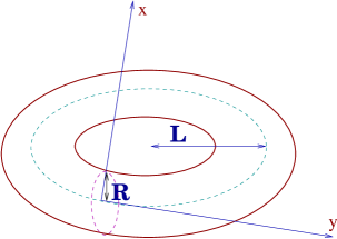
Figure 3.1: Torus generated by two circles of circumferences ${R}$ and ${L}$.

i) as a first choice, we may consider the $y$ axis as the one playing the role of time direction and let $L\rightarrow\infty$ with $R$ remaining finite. Then, if we denote by $H_{R}$ the hamiltonian describing the system in the compactified (periodic) space of dimension $R$ and by $\mathcal{H}_{R}$ the corresponding Hilbert space, the partition function associated to the field theory $\mathcal{Z}(R,L)$ is given by,

$$\mathcal{Z}(R,L)=\lim_{L\rightarrow\infty}\textnormal{Tr}_{\mathcal{H}_{R}}e^{-LH_{R}}\approx e^{-E_{0}(R)L},$$ (3.24)

for $E_{0}(R)$ to be the energy of the ground state, since in the limit $L\rightarrow\infty$, the term associated to the eigenstate of minimum energy of the Hamiltonian $H_{R}$ is the dominant contribution to the partition function $\mathcal{Z}(R,L)$,

ii) alternatively we could exchange the roles of the axis $x$, $y$ and associate them now to the time and space dimensions respectively. Hence, if we now perform the same limit carried out in i), namely we take $L\rightarrow\infty$ we are in a new situation in which the theory is time-periodic, with periodicity given by $R$. Moreover, if we identify the dimension $R$ as the same quantity occurring in the thermodynamic Bethe ansatz equations (3.20), namely the inverse temperature $R=1/T$, our alternative choice of axis is equivalent to a formulation of the QFT at finite temperature. Therefore, denoting by $H_{L}$ the new hamiltonian and by $\mathcal{H}_{L}$ the corresponding Hilbert space, the partition function $\mathcal{Z}(R,L)$ is now given by

$$\mathcal{Z}(R,L)=\lim_{L\rightarrow\infty}\textnormal{Tr}_{\mathcal{H}_{L}}e^{-RH_{L}}\approx e^{-RLf(R)},$$ (3.25)

where $f(R)$ is the free energy per unit length of the system at finite temperature $T=1/R$ namely, the same function obtained in (3.23).

iii) Putting now together the results coming from i) and ii) we obtain a relationship between the extremal free energy (3.23) and the ground state energy $E_{0}(R)$ which is simply

$$Rf(R)=E_{0}(R).$$ (3.26)

We are now able to extract information about the underlying CFT by performing the ultraviolet limit $R=1/T\rightarrow 0$. In this limit the partition function $\mathcal{Z}(R,L)$ must reduce to the one of the underlying CFT on a cylinder, as the limit $L\rightarrow\infty$ is nothing but the limit torus $\rightarrow$ infinite cylinder. Consequently, it is necessary at this point to make use of some basic notions of conformal field theory on a cylinder which for this purpose have been introduced in subsection 2.1.1 of the previous chapter. The results presented there guarantee that a relationship between the ground state energy $E_{0}(R)$, related to the equilibrium free energy by means of (3.26), and the energy of the eigenstates of the hamiltonian (2.38) can be now established. Clearly such a relationship arises in the UV limit in which the QFT studied in the previous subsections reduces to its underlying CFT on a cylinder of infinite length $L\rightarrow\infty$ and time dimension $R=1/T$. In the ultraviolet limit we obtain

$$\lim_{R\rightarrow 0}Rf(R)=-\frac{\pi}{6R}c_{eff}\,\,\,\,\,\,\,\,\textnormal{with}\,\,\,\,\,\,\,\,c_{eff}:=c-12(\Delta_{0}+\bar{\Delta}_{0}),$$ (3.27)

where $\Delta_{0},\bar{\Delta}_{0}$ are the lowest conformal dimensions related to the two chiral sectors. The latter relationship was originally derived in [23]. The quantity $c_{eff}$ is known as effective central charge and for unitary CFT’s coincides with the Virasoro central charge $c$, since the conformal dimensions $\Delta_{0},\bar{\Delta}_{0}$ are zero. Since the WZNW-coset models are unitary CFT’s, this will be the case for the HSG-models. Therefore, the introduction of periodic boundary conditions in a unitary CFT has the effect of generating a non-zero value for the ground state energy in the UV-limit and in that sense the effective central charge can be interpreted as Casimir energy.

The relation (3.27) will be fundamental for our TBA-analysis. Recall that the initial motivation for such an analysis was the search for consistency checks of the S-matrix proposal [51] for the HSG-models, checks which will exploit the interpretation of these models as perturbed coset theories. Therefore, having solved the TBA-equations (3.20) and extracted the corresponding $L$-functions we may introduce then in (3.23) and perform the corresponding integrals while carrying out the UV-limit. Proceeding this way we may have identified the Virasoro central charge of the original CFT. Since the HSG-models, like many other 1+1-dimensional integrable QFT’s, have been constructed as perturbations of a well-known CFT, the Virasoro central charge extracted from our analysis may be directly compared with its expected value ( see Eq. (2.123)).

However, this is not the only information we can extract from a TBA-analysis. In a similar fashion we defined the effective central charge $c_{eff}$ through (3.27) we can define a new function $c(R)$ which we will refer to as finite size scaling function,

$$c(R)=-\frac{6R^{2}}{\pi}f(R)=\frac{3R}{\pi^{2}}\sum_{A=1}^{n}M_{A}\int\limits_{-\infty}^{\infty}{d\theta}L_{A}(\theta)\cosh\theta.$$ (3.28)

In comparison to (3.27) the function $E_{0}(R)=-\pi c(R)/6R$ can be interpreted as “off-critical ” Casimir energy [21, 116]. It is clear that in the UV-limit,

$$\lim_{R\rightarrow 0}c(R)=c_{eff}=c-12(\Delta_{0}+\bar{\Delta}_{0}).$$ (3.29)

Thus, the solution of the TBA-equations (3.20) does not only allow for the identification of the Virasoro central charge of the underlying CFT but also for the computation (usually numerically) of the function $c(R)$ defined in (3.28). It is also expected that for a massive QFT the IR-limit of the finite size scaling function must be zero, and in the intermediate region $0<R<\infty$ it should provide information about the onset of the stable and unstable particles of the model i.e., the energy scale $R$ at which these particles can be formed. In particular, it will be shown later for the HSG-models that, for finite values of $R$, the scaling function $c(R)$ exhibits a very characteristic “staircase” pattern where the number of steps is determined by the number of free parameters in the model and is also related to the number of particles present in the theory. Such a behaviour was observed previously for the roaming sinh-Gordon model [108] and their generalisations [109, 110]. This behaviour suggests that, similarly to the well-known Zamolodchikov’s $c$-function [24], which we will compute in the context of the form factor program, the scaling function admits an interpretation as a measure of effective light degrees of freedom. In other words, starting in the deep UV-limit which corresponds to the situation in which the mass of any of the particles of the theory is much lower than the energy scale, and therefore they all can be formed and contribute to the Virasoro central charge $c$, we will observe the consecutive “decoupling” of the heaviest particles of the theory as soon as an energy scale much lower than the energy precise for their production is reached. Finally, in the IR-limit none of the particles can be formed and the scaling function will vanish. It is then clear that the information provided by the scaling function is crucial concerning the check of the physical picture expected for the HSG-models [48, 49, 50, 63, 90]. Recall that the S-matrix proposal [51] was based on the extrapolation of semi-classical results, in particular concerning the stable and unstable particle spectrum therefore, from that point of view, the outlined interpretation of the “staircase” behaviour of the scaling function provides strong support for the validity of the mentioned assumptions. It must be emphasised that such a clear physical interpretation is not possible for the mentioned roaming sinh-Gordon models [108, 109, 110], amongst other reasons, due to the lack of a consistent Lagrangian formulation.

We have now all the necessary ingredients to carry out our specific application of the TBA-approach for the the HSG-models. The main features of these theories have been already stated in subsection 2.4.2 of the previous chapter. As a fundamental input in the TBA-framework the knowledge of the two-particle scattering amplitudes and mass spectrum is needed. Also, some of the most characteristic data of the associated underlying coset CFT, like the Virasoro central charge (2.123) and the dimension of the perturbing field (2.121) have been reported in the previous chapter and we will frequently appeal to their expected values in the course of our TBA-analysis.

3.2 TBA with parity violation and resonances

In this section we are going to determine the conformal field theory which governs the UV-regime of the QFT associated with the S-matrix elements (2.143) and (2.146). According to the defining relation (2.111) and the discussion of the previous section, we expect to recover the WZNW-coset theory with effective central charge (2.123) in the extreme UV-limit by means of a TBA-analysis. Since up to now such an analysis has only been carried out for parity invariant S-matrices, a few comments are due to implement parity violation. Recall that the starting point in the derivation of the key equations are the Bethe ansatz equations, which are the outcome of dragging one soliton, say of type $A=(a,i)$, along the world line. For the time being we do not need the distinction between the two quantum numbers. On this trip the formal wave-function of $A$ picks up the corresponding S-matrix element as a phase factor when meeting another soliton (see subsection 3.1.1). Due to the parity violation it matters, whether the soliton is moved clockwise or counter-clockwise along the world line, such that instead of the set of equations (3.5) we end up with two apparently different sets of Bethe Ansatz equations

$$e^{iLM_{A}\sinh\theta_{A}}\prod\limits_{B\neq A}S_{AB}(\theta_{A}-\theta_{B})=1\quad\text{and \quad}e^{-iLM_{A}\sinh\theta_{A}}\prod\limits_{B\neq A}S_{BA}(\theta_{B}-\theta_{A})=1\,,$$ (3.30)

with $L$ denoting the length of the compactified space direction. These two sets of equations are of course not entirely independent and may be obtained from each other by complex conjugation with the help of the properties of unitarity and Hermitian analyticity of the S-matrix (2.88) summarised in the previous chapter. We may carry out the thermodynamic limit of (3.30) in the usual fashion [21] as described in subsection 3.1.2 and obtain the following sets of non-linear integral equations

$$\epsilon_{A}^{+}(\theta)+\sum_{B}\,\Phi_{AB}*L_{B}^{+}(\theta) = r\,M_{A}\cosh\theta,\quad$$ (3.31)

$$\epsilon_{A}^{-}(\theta)+\sum_{B}\,\Phi_{BA}*L_{B}^{-}(\theta) = r\,M_{A}\cosh\theta\,\,\,.$$ (3.32)

Here $r=m_{1}T^{-1}$ is the inverse temperature times the overall mass scale $m_{1}$ of the lightest particle and we also re-defined the masses by $M_{a}^{i}\rightarrow M_{a}^{i}/m_{1}$ keeping, however, the same notation. As pointed out before, it is useful in these considerations to introduce the so-called pseudo-energies $\epsilon_{A}^{+}(\theta)=\epsilon_{A}^{-}(-\theta)$ and the related functions

$$L_{A}^{\pm}(\theta)=\ln(1+e^{-\epsilon_{A}^{\pm}(\theta)}).$$ (3.33)

Notice that (3.32) may be obtained from (3.31) simply by the parity transformation $\theta\rightarrow-\theta$ and the first equality in (3.11). The main difference of these equations in comparison with the parity invariant case is that we have lost the usual symmetry of the pseudo-energies as functions of the rapidities, such that we have now in general $\epsilon_{A}^{+}(\theta)\neq\epsilon_{A}^{-}(\theta)$. This symmetry may be recovered by restoring parity.

It is also worth mentioning that according to (3.21) the $L$-functions (3.33) imply that we have chosen the statistical interaction to be of fermionic type. This choice has been made for all the theories studied in the TBA-context until now and relies on the fact that the S-matrix describing the interaction between identical particles namely, particles with the same quantum numbers and momenta is given by

$$S_{aa}^{ii}(0)=-1,$$ (3.34)

as follows from (2.142). Therefore, it coincides with the S-matrix describing the interaction between free fermions. This choice is not in contradiction with the bosonic character of the field $h(x^{0},x^{1})$ entering the action (2.111) and should not lead to confusion. In particular it is a well-known fact that in $1+d$-dimensions, with $d<3$ there is not an intrinsic meaning for the statistics and any QFT described in terms of bosonic fields admits also a description in terms of fermionic fields which only involves a suitable field transformation. Examples of such an “ambiguity” are provided by [122]. Concerning the role of the statistics in the TBA-context, in [118] the TBA-approach was formulated for a more general choice of the statistics known as Haldane statistics [123]. It was observed also in [118] that essentially any choice of the statistical interaction can be made leading to the same TBA-equations, if it is suitably compensated by a particular change in the phase of the S-matrix. Therefore, in the TBA-context we could extract the same information i.e., central charge, scaling function… even if we decided to choose a more “exotic” type of statistics, provided the S-matrix proposal was modified as suggested in [118]. Very recently [124], the TBA-approach has been generalised for Gentile statistics [125] along the same lines of [118].

The scaling function, may be computed similar as in (3.28)

$$c(r)=\frac{3\,r}{\pi^{2}}\sum_{A}M_{A}\int\limits_{0}^{\infty}d\theta\,\cosh\theta\,(L_{A}^{-}(\theta)+L_{A}^{+}(\theta))\,,$$ (3.35)

where we only used the property $L_{+}(\theta)=L_{-}(-\theta)$ to substitute the integral $\int_{-\infty}^{\infty}$ in (3.28) by $\int_{0}^{\infty}$ in (3.35). As we have seen in subsection 3.1.2, once the equations (3.31), (3.32) have been solved for the pseudo-energies $\epsilon_{A}^{\pm}$, of special interest is the deep UV-limit, i.e. $r\rightarrow 0$ in which, according to (3.29) we expect to identify the Virasoro central charge (2.123) of the underlying CFT. This assumption will turn out to be consistent with the analytical and numerical results.

3.2.1 Ultraviolet central charge for the HSG-models

In this section we follow the usual argumentation of the TBA-analysis [21] which leads to the effective central charge, paying, however, attention to the parity violation. We will recover indeed the value in (2.123) as the central charge of the HSG-models. In fact, following [21] we will be able to determine the effective central charge analytically when performing the limit $r\rightarrow 0$ in (3.35). The reason is that in this limit there will be various terms both in (3.35) and (3.31) which we can safely neglect and consequently, the evaluation of both expressions becomes simpler.

It is useful at this point to introduce the new variable $x=\ln(r/2)$ so that the UV-limit corresponds now to $x\rightarrow-\infty$. In this limit the factor $rM_{A}\cosh\theta$ arising both in the integral (3.35) and in the TBA-equations (3.31), (3.32) can be approximated in the following way,

$$rM_{A}\cosh\theta={M_{A}}\Big{(}e^{\theta+x}+e^{-\theta+x}\Big{)}\simeq{M_{A}}e^{\arrowvert\theta\arrowvert+x},$$ (3.36)

Here we find for the first time the occurrence of the term $M_{A}e^{x+\theta}$ in our analysis, which arises naturally in the formulation the TBA-equations for massless particles. The concept of massless scattering has been introduced originally in [126] as follows: The on-shell energy of a right and left moving particle is given by $E_{\pm}=M/2\,e^{\pm\theta}$ which is formally obtained from the on-shell energy of a massive particle $E=m\cosh\theta$ by the replacement $\theta\rightarrow\theta\pm\sigma/2$ and taking the limit $m\rightarrow 0,\sigma\rightarrow\infty$, while keeping the expression $M=m\,e^{\sigma/2}$ finite. We will encounter these on-shell energies in the course of our analysis.

The substitution of (3.36) into the expression for the scaling function (3.35) gives

$$c(r)\simeq\frac{3}{\pi^{2}}\sum_{A}M_{A}\int\limits_{0}^{\infty}d\theta\,e^{\theta+x}\,(L_{A}^{-}(\theta)+L_{A}^{+}(\theta))=\frac{3}{\pi^{2}}\sum_{A}M_{A}\int\limits_{x}^{\infty}d\theta\,e^{\theta}\,(L_{A}^{\small{>}}(\theta)+L_{A}^{\small{<}}(\theta)).$$ (3.37)

The second equality in (3.37) is simply obtained by shifting $\theta\rightarrow\theta+x$ and defining the so-called “kink” functions

$$L_{A}^{\small{>}}(\theta):=L_{A}^{+}(\theta-x),\,\,\,\,\,\,\,\,\,\,\,\,\,\,\,\,\textnormal{and}\,\,\,\,\,\,\,\,\,\,\,\,\,\,\,\,L_{A}^{\small{<}}(\theta):=L_{A}^{-}(\theta-x),$$ (3.38)

originally introduced in [21].

We can now carry out the same limit for the TBA-equations (3.31), (3.32),

$$M_{A}e^{\theta} \simeq \epsilon_{A}^{\small{>}}(\theta)+\sum_{B}\,\Phi_{AB}*L_{B}^{>}(\theta),$$ (3.39)

$$M_{A}e^{\theta} \simeq \epsilon_{A}^{\small{<}}(\theta)+\sum_{B}\,\Phi_{BA}*L_{B}^{\small{<}}(\theta),$$ (3.40)

where the approximation (3.36) has been used again. Taking now the derivative with respect to $\theta$ of the latter equations and using (3.11) and (3.12) we obtain

$$M_{A}e^{\theta} \simeq \frac{d\epsilon_{A}^{>}}{d\theta}+\sum_{B}\int\limits_{-\infty}^{\infty}\frac{d\theta^{\prime}}{2\pi}{\Phi_{AB}(\theta-\theta^{\prime})}\frac{dL_{B}^{>}(\theta^{\prime})}{d\theta^{\prime}},$$ (3.41)

$$M_{A}e^{\theta} \simeq \frac{d\epsilon_{A}^{<}}{d\theta}+\sum_{B}\int\limits_{-\infty}^{\infty}\frac{d\theta^{\prime}}{2\pi}{\Phi_{AB}(-\theta+\theta^{\prime})}\frac{dL_{B}^{<}(\theta^{\prime})}{d\theta^{\prime}}.$$ (3.42)

Notice that in the convolution terms the derivative with respect to $\theta$ has been substituted by a derivative with respect to $\theta^{\prime}$. This can be done using integration by parts and the trivial fact

$$\frac{d}{d\theta}\Phi_{AB}(\theta-\theta^{\prime})=-\frac{d}{d\theta^{\prime}}\Phi_{AB}(\theta-\theta^{\prime}).$$ (3.43)

Having Eqs. (3.41) and (3.42) at hand, it is possible to substitute the term $M_{A}e^{\theta}$ in (3.37) by the r.h.s. of these equations. By doing so, we obtain

$$\sum_{A}M_{A}\int\limits_{x}^{\infty}d\theta e^{\theta}L_{A}^{>}(\theta)=\sum_{A}M_{A}\int\limits_{x}^{\infty}d\theta L_{A}^{>}(\theta)\frac{d\epsilon_{A}^{>}}{d\theta}+\sum_{A,B}\int\limits_{x}^{\infty}L_{A}^{>}(\theta)\,\Phi_{AB}*(L_{B}^{>})^{\prime}(\theta),$$ (3.44)

where $(L_{A}^{>})^{\prime}$ denotes the derivative of the $L_{A}^{>}$ function. Obviously a completely analogous equation can be obtained for the other contribution to (3.37) by using (3.42).

Let us now look separately at each of the two contributions in (3.44). Using (3.33) it is trivial to see that the first one is simply

$$\sum_{A}M_{A}\int\limits_{x}^{\infty}d\theta\frac{d\epsilon_{A}^{>}}{d\theta}L_{A}^{>}(\theta)=\sum_{A}M_{A}\int\limits_{\epsilon_{A}^{>}(x)}^{\epsilon_{A}^{>}(\infty)}d\epsilon_{A}^{>}\ln(1+e^{\epsilon_{A}^{>}(\theta)}),$$ (3.45)

whereas for the second one we obtain

$$\sum_{A,B}\int\limits_{x}^{\infty}d\theta\,L_{A}^{>}(\theta)\,\Phi_{AB}*(L_{A}^{>})^{\prime}(\theta) = \sum_{A,B}\int\limits_{x}^{\infty}\frac{d\theta^{\prime}}{2\pi}\int\limits_{-\infty}^{\infty}d\theta\,L_{B}(\theta^{\prime})\Phi_{AB}(\theta-\theta^{\prime})\frac{dL_{A}(\theta)}{d\theta}$$ (3.46)

$$\simeq \sum_{A,B}\int\limits_{x}^{\infty}d\theta\frac{L_{A}^{>}(\theta)}{d\theta}\Phi_{AB}*L_{A}^{>}(\theta).$$

Here we used the approximation $\int_{x}^{\infty}\simeq\int_{-\infty}^{\infty}$ to obtain the last equality and the fact that there is a summation over the indices $A,B$, so that their names can safely be interchanged and similarly for the integration variables $\theta$, $\theta^{\prime}$. It is also necessary to take the first property in (3.11) into account together, of course, with the definition of the convolution (3.12). However, it is possible to express (3.46) still in a more suitable way by using now the approximated TBA-equation (3.39) to eliminate the convolution term and the defining relation (3.33) of the $L$-functions in terms of the pseudo-energies

$$\sum_{A,B}\int\limits_{x}^{\infty}d\theta\frac{L_{A}^{>}(\theta)}{d\theta}(\Phi_{AB}*L_{A}^{>})(\theta)\simeq\sum_{A}\int\limits_{\epsilon_{A}^{>}(x)}^{\epsilon_{A}^{>}(\infty)}d\epsilon_{A}^{>}\frac{\epsilon_{A}^{>}}{(1+e^{\epsilon_{A}^{>}})}-\sum_{A}\int\limits_{x}^{\infty}d\theta M_{A}e^{\theta}L_{A}^{>}(\theta).$$ (3.47)

Notice that the last term on the r.h.s., which is obtained after integration by parts, is precisely our starting point (3.44). Therefore, substituting the contributions (3.45) and (3.47) into (3.44) we obtain

$$\int\limits_{x}^{\infty}d\theta M_{A}e^{\theta}L_{A}^{>}(\theta)=\frac{1}{2}\int\limits_{\epsilon_{A}^{>}(x)}^{\epsilon_{A}^{>}(\infty)}d\epsilon_{A}^{>}\,M_{A}\ln(1+e^{\epsilon_{A}^{>}(\theta)})+\frac{1}{2}\int\limits_{\epsilon_{A}^{>}(x)}^{\epsilon_{A}^{>}(\infty)}d\epsilon_{A}^{>}\,\frac{\epsilon_{A}^{>}}{(1+e^{\epsilon_{A}^{>}})}.$$ (3.48)

A similar expression can be obtained for the second term in (3.37) so that, we can finally write

$$\lim_{r\rightarrow 0}\,c(r)\simeq\frac{3}{2\pi^{2}}\sum\limits_{p=+,-}\sum_{A}\int\limits_{\epsilon_{A}^{p}(0)}^{\epsilon_{A}^{p}(\infty)}d\epsilon_{A}^{p}\left[\ln(1+e^{-\epsilon_{A}^{p}})+\frac{\epsilon_{A}^{p}}{1+e^{\epsilon_{A}^{p}}}\right]\,\,\,,$$ (3.49)

where we use again the standard pseudo-energies $\epsilon_{A}^{\pm}$ instead of the “kink ” variables (3.38) and consequently substitute

$$\epsilon_{A}^{+}(0)=\epsilon_{A}^{>}(x)\,\,\,\,\,\,\,\,\,\,\,\,\,\,\,\textnormal{and}\,\,\,\,\,\,\,\,\,\,\,\,\,\,\,\epsilon_{A}^{-}(0)=\epsilon_{A}^{<}(x).$$ (3.50)

Upon the substitution $y_{A}^{p}=1/(1+\exp(\epsilon_{A}^{p}))$ we obtain the following expression for the effective central charge

$$c_{\text{eff}}=\lim_{r\rightarrow 0}\,c(r)=\frac{6}{\pi^{2}}\sum_{A}\mathcal{L}\left(\frac{1}{1+e^{\epsilon_{A}^{\pm}(0)}}\right)\,\,.$$ (3.51)

Here we used the integral representation for Roger’s dilogarithm function

$$\mathcal{L}(x)=1/2\int_{0}^{x}dy\Bigg{(}\frac{\ln y}{(y-1)}-\frac{\ln(1-y)}{y}\Bigg{)},$$ (3.52)

and the fact that $\epsilon_{A}^{+}(0)=\epsilon_{A}^{-}(0)$, $y_{A}^{+}(\infty)=y_{A}^{-}(\infty)=0$. Comparing Eq. (3.51) with the equivalent expression obtained in the parity invariant case (see e.g. [21]), we conclude that we end up precisely with the same situation: Having solved the TBA-equations (3.39) and (3.40), we may compute the effective central charge in terms of Roger’s dilogarithm thereafter. Notice that in the ultraviolet limit we have recovered the parity invariance and (3.51) holds for all finite values of the resonance parameter. Notice also that, in fact, in order to compute the effective central charge (3.51) we do not need to solve the TBA-equations (3.39), (3.40) for any value of $\theta$, since only the values of the pseudo-energies at zero rapidity enter the expression (3.51). Therefore, let us now consider the limit $\theta\rightarrow 0$ of Eqs. (3.39) and (3.40).

When we assume that the kernels $\Phi_{AB}(\theta)$ are strongly peaked at $\theta=0$ and develop the characteristic plateaux one observes for the scaling models, we can take out the $L$-functions from the integral in the equations (3.39), (3.40) and obtain

$$\epsilon_{A}^{\pm}(0)+\sum_{B}\,N_{AB}L_{B}^{\pm}(0)=0\qquad\quad\text{with \quad}N_{AB}=\frac{1}{2\pi}\int\limits_{-\infty}^{\infty}d\theta\,\,\Phi_{AB}(\theta)\,\,,$$ (3.53)

where we again appeal to (3.50). Note that in (3.53) we have recovered the parity invariance.

Having the resonance parameter $\sigma$ present in our theory we may also encounter a situation in which $\Phi_{AB}(\theta)$ is peaked at $\theta=\pm\sigma$. This means in order for (3.53) to be valid, we have to assume $\epsilon_{A}^{\pm}(0)=\epsilon_{A}^{\pm}(\pm\sigma)$ in the limit $r\rightarrow 0$ in addition, to accommodate that situation. This assumption will be justified for particular cases from the numerical results (see e.g. Fig. 3.2), but can also be derived from analytical considerations which make use of Eqs. (3.39) and (3.40). Recall that these equations have been obtained as the UV-limit of the original TBA-equations (3.31), (3.32). Obviously, since $x\rightarrow-\infty$, the condition $|\sigma|\ll x$ is always guaranteed in the UV-regime. At the same time, footnote 1 shows that the kernels $\Phi_{AB}(\theta)$ are strongly peaked either at $\theta=0$ or $\theta=\pm\sigma$. Therefore, one can safely approximate the convolution term in (3.39) at $\theta=x$ by

$$\Phi_{AB}*L_{B}^{>}(x)\simeq\Big{(}\int_{-\infty}^{\infty}\frac{dy}{2\pi}\Phi_{AB}(y)\Big{)}L_{B}^{>}(x)=N_{AB}L_{B}^{>}(x),$$ (3.54)

and analogously for (3.40). The substitution of (3.54) in (3.39) and equivalently in (3.40) leads to Eqs. (3.53) with the help of definitions (3.38).

For the case at hand we read off from the integral representation of the scattering matrices (2.143) and (2.146)

$$N_{AB}=N_{ab}^{ij}=\delta_{ij}\delta_{ab}-K_{ij}^{g}\,(K^{A_{k-1}})_{\,\,\,\,\,\,\,\,\,ab}^{-1}\,\,,$$ (3.55)

for $K^{g}$ and $K^{A_{k-1}}$ to be the Cartan matrices of $g$ and $A_{k-1}$ respectively.

With $N_{ab}^{ij}$ in the form (3.55) and the identifications

$$Q_{a}^{i}:=\prod_{b=1}^{k-1}(1+\exp(-\epsilon_{b}^{i}(0)))^{K_{ab}^{-1}},$$ (3.56)

the constant TBA-equations (3.53) are precisely the equations which occurred before in the context of the restricted solid-on-solid models [127, 128, 129, 130, 131]. It was noted in there that (3.53) may be solved elegantly in terms of Weyl-characters and the reported effective central charge coincides indeed with the one for the HSG-models (2.123). This is a highly non-trivial result which provides determinant support for the S-matrix proposal [51], since the ultraviolet central charge of all the parafermionic theories related to the cosets $G_{k}/U(1)^{\ell}$ is precisely reproduced. Also, from a purely mathematical point of view, the fact that the quantity $c_{eff}$ given by Eq. (3.51) is a rational number is quite exceptional. When this happens, the system (3.53) and (3.51) is known under the special name of accessible dilogarithms. A more general set of $N$-matrices, containing (3.55) as a particular example, was obtained in the context of the $g|\tilde{g}$-theories [67].

It should be noted that we understand the $N$-matrix here as defined in (3.53) and not as the difference between the phases of the S-matrix. In the latter case we encounter contributions from the non-trivial constant phase factors $\eta$. Also in that case we may arrive at the same answer by compensating them with a choice of a non-standard statistical interaction [118] as outlined in section 3.2.

We would like to close this section with a comment which links our analysis to structures which may be observed directly inside the conformal field theory. When one carries out a saddle point analysis, see e.g. [133, 134], on a Virasoro character of the general form

$$\chi(q)=\sum\limits_{\vec{m}=0}^{\infty}\frac{q^{\frac{1}{2}\vec{m}(\mathbf{1}-N)\vec{m}^{t}+\vec{m}\cdot\vec{B}}}{(q)_{1}\ldots(q)_{(k-1)\text{$\ell$}}}\,\,,$$ (3.57)

with $(q)_{m}=\prod_{k=1}^{m}(1-q^{k})$, one recovers the set of coupled equations as (3.53) and the corresponding effective central charge is expressible as a sum of Roger’s dilogarithms as (3.51). Note that when we choose $g\equiv A_{1}$ the HSG-model reduces to the minimal ATFT and (3.57) reduces to the character formulae in [169]. Thus the equations (3.53) and (3.51) constitute an interface between massive and massless theories, since they may be obtained on one hand in the ultraviolet limit from a massive model and on the other hand from a limit inside the conformal field theory. This means we can guess a new form of the coset character, by substituting (3.55) into (3.57). However, since the specific form of the vector $\vec{B}$ does not enter in this analysis (it distinguishes the different highest weight representations) more work needs to be done in order to make this more than a mere conjecture. Further results in this direction have been provided in [135].

3.3 Thermodynamic Bethe ansatz for the ${SU(3)_{k}}$-HSG model

We shall now focus our discussion on $G=SU(3)_{k}$. First of all we need to establish how many free parameters we have at our disposal in this case. According to the discussion in subsection 2.4.2 we can tune the resonance parameter and the mass ratio

$$\sigma:=\sigma_{21}=-\sigma_{12}\quad\text{and}\quad m_{1}/m_{2}\,\,.$$ (3.58)

It will also be useful to exploit a symmetry present in the TBA-equations related to $SU(3)_{k}$ by noting that the parity transformed equations (3.32) turn into the equations (3.31) when we exchange the masses of the different types of solitons. This means the system remains invariant under the simultaneous transformations

$$\theta\rightarrow-\theta\quad\quad\text{and\qquad}m_{1}/m_{2}\rightarrow m_{2}/m_{1}\,\,.$$ (3.59)

For the special case $m_{1}/m_{2}=1$ we deduce therefore that $\epsilon_{a}^{1}(\theta)=\epsilon_{a}^{2}(-\theta)$, meaning that a parity transformation amounts to an interchange of the colours. Furthermore, we see from (3.32) and the defining relation $\sigma=\sigma_{21}=-\sigma_{12}$ that changing the sign of the rapidity variable is equivalent to $\sigma\rightarrow-\sigma$. Therefore, we can restrict ourselves to the choice $\sigma\geq 0$ without loss of generality.

3.3.1 Staircase behaviour of the scaling function

We will now come to the evaluation of the scaling function (3.35) for finite and small scale parameter $r$. To do this we have to solve first the TBA equations (3.31) for the pseudo-energies, which up to now has not been achieved analytically for systems with a non-trivial dynamical interaction due to the non-linear nature of the integral equations. Nonetheless, numerically this problem can be controlled relatively well. In [113] a rigorous proof of the existence and uniqueness of solutions to TBA-equations of the type (3.31), (3.32) was provided. Before [113] such properties were simply assumed to hold in the light of the consistent analytical and numerical results obtained. However, the proof provided in [113] is very relevant since if the equations (3.31), (3.32) allowed several different solutions for the pseudo-energies $\epsilon_{A}^{\pm}(\theta)$, different values for the effective central charge could be obtained starting with the same S-matrix and statistics and, consequently, the results of the TBA-analysis would not provide a reliable consistency check of the mentioned S-matrix.

In the UV-regime, for $r\ll 1$, one is in a better position and can set up approximate TBA-equations involving, formally, massless particles, for which various approximation schemes have been developed which depend on the general form of the $L$-functions. Since those functions are not known a priori, one may justify ones assumptions in retrospect by referring to the numerics. In section 3.4 we present numerical solutions for the equations (3.31) for various levels $k$ showing that the $L$-functions develop at most two (three if $m_{1}$ and $m_{2}$ are very different) plateaux in the range $x<\theta<-x$ and then fall off rapidly (see Fig. 3.2). This type of behaviour is similar to the one known from minimal ATFT [21, 132], and we can therefore adopt various arguments presented in that context. The main difficulty we have to deal with here is to find the appropriate “massless” TBA equations accommodating the dependence of the TBA equations on the resonance shifts $\sigma$.

We start by giving also an integral representation for the kernel (3.11). This representation can be obtained from the integral representation of the two-point scattering matrices (2.143), (2.146) by using the same kind of arguments presented in [113] for ATFT’s related to simply laced Lie algebras. Moreover, we can separate the kernel (3.11) into two parts

$$\phi_{ab}(\theta) = \Phi_{ab}^{ii}(\theta)=\int dt\,\left[\delta_{ab}-2\cosh\tfrac{\pi t}{k}\left(2\cosh\tfrac{\pi t}{k}-I\right)_{ab}^{-1}\right]\,e^{-it\theta}\;,\quad$$ (3.60)

$$\psi_{ab}(\theta) = \Phi_{ab}^{ij}(\theta+\sigma_{ji})=\int dt\,\left(2\cosh\tfrac{\pi t}{k}-I\right)_{ab}^{-1}\,e^{-it\theta}\;\,\,,i\neq j,\,\,\,K_{ij}^{g}=-1.$$ (3.61)

Here $\phi_{ab}(\theta)$ is just the TBA-kernel of the $A_{k-1}$-minimal ATFT [113] and in the remaining kernel $\psi_{ab}(\theta)$ we have removed the resonance shift. Note that $\phi,\psi$ do not depend on the colour values $i,j$ and may therefore be dropped all together in the notation. They are generically valid for all values of the level $k$. The convolution term in (3.31) in terms of $\phi,\psi$ is then re-written as

$$\sum_{j=1}^{\ell}\sum_{b=1}^{k-1}\Phi_{ab}^{ij}*L_{b}^{j}(\theta)=\sum_{b=1}^{k-1}\phi_{ab}*L_{b}^{i}(\theta)+\sum\Sb j=1\\ j\neq i\endSb^{\ell}\sum_{b=1}^{k-1}(\psi_{ab}*L_{b}^{j})(\theta-\sigma_{ji})\,.$$ (3.62)

These equations illustrate that whenever we are in a regime in which the second term in (3.62) is negligible we are left with $\ell$ non-interacting copies of the $A_{k-1}$-minimal ATFT. In other words, whenever the resonance parameters $\sigma_{ij}$ become very big, the unstable particles can not be formed anymore so that all the two-particle scattering amplitudes satisfy Eq. (LABEL:and1) and we have $\ell$ copies of minimal $A_{k-1}$-ATFT.

We will now specialise the discussion on the $SU(3)_{k}$-case for which it is very useful to perform the shifts $\theta\rightarrow\theta\pm\sigma/2$ in the TBA-equations. In the UV-limit $r\rightarrow 0$ with $\sigma\gg 1$ the shifted functions can be approximated by the solutions of the following sets of integral equations

$$\varepsilon_{a}^{\pm}(\theta)+\sum_{b=1}^{k-1}\phi_{ab}*L_{b}^{\pm}\left(\theta\right)+\sum_{b=1}^{k-1}(\psi_{ab}*L_{b}^{\mp})\left(\theta\right) = r^{\prime}\,M_{a}^{\pm}\,e^{\pm\theta}\quad\,$$ (3.63)

$$\hat{\varepsilon}_{a}^{\pm}(\theta)+\sum_{b=1}^{k-1}(\phi_{ab}*\hat{L}_{b}^{\pm})\left(\theta\right) = r^{\prime}\,M_{a}^{\mp}\,\,e^{\pm\theta}\,,\quad$$ (3.64)

where we have introduced the parameter $r^{\prime}=r/2\,e^{\sigma/2}=e^{x+\sigma/2}$ familiar from the discussion of massless scattering [126] and the masses $M_{a}^{+/-}=M_{a}^{1\,/\,2}$. Notice that the indices “+”, “-” in the pseudo-energies and $L$-functions have nothing to do with the same indices used in section 3.2. Now, these labels refer to the two different possible colour indices $i=1,2$, since the rank of the Lie algebra $su(3)$ is $\ell=2$ and the functions $\varepsilon_{a}^{\pm}(\theta)$ are in fact related to the original ones $\epsilon_{a}^{i}(\theta)=$$\epsilon_{A}(\theta)=$$\epsilon_{A}^{+}(\theta)$ by means of a rapidity shift, in a similar fashion to the “kink” equations (3.38) introduced in subsection 3.2.1. The same relationship holds for the functions $\hat{\varepsilon}_{a}^{\pm}$ which make sense in a different regime of values of the parameters $r,\sigma$. More precisely, the relationship between the solutions of the system (3.63), (3.64) and those of the original TBA-equations is given by

$$\varepsilon_{a}^{+|-}(\theta) = \epsilon_{a}^{1|2}(\theta\pm\sigma/2)\qquad\text{for\quad}x\ll\pm\theta\ll x+\sigma$$ (3.65)

$$\hat{\varepsilon}_{a}^{+|-}(\theta) = {\epsilon}_{a}^{1|2}(\theta\pm\sigma/2)\qquad\text{for\quad}\pm\theta\ll\min[-x,x+\sigma].$$ (3.66)

where we have assumed the equality of the mass scales i.e, $m_{1}=m_{2}$. Similar equations may be written down for the generic case. The approximations leading to (3.63), (3.64) follow similar lines as the ones involved in the derivation of Eq. (3.51), with the difference that now two parameters $x,\sigma$ are involved in the discussion and their relative value has to be taken into account in order to establish which terms are negligible and which are not in the mentioned limit $r\rightarrow 0,\sigma\gg 1$.

In deriving (3.66) we have neglected the convolution terms $(\psi_{ab}*L_{b}^{1})(\theta+\sigma)$ and $(\psi_{ab}*L_{b}^{2})(\theta-\sigma)$ which appear in the TBA-equations for $\epsilon_{a}^{2}(\theta)$ and $\epsilon_{a}^{1}(\theta)$, respectively. This is justified by the following argument: For $|\theta|\gg$ $-x$ the free on-shell energy term is dominant in the TBA equations, i.e. $\epsilon_{a}^{i}(\theta)\approx r\,M_{a}^{i}\cosh\theta\simeq M_{a}^{i}e^{|\theta|+x}$ and the functions $L_{a}^{i}(\theta)$ are almost zero. The kernels $\psi_{ab}$ are centered in a region around the origin $\theta=0$ outside of which they exponentially decrease (see footnote in subsection 3.2.1 for an explanation of this). This means that the convolution terms in question can be neglected safely if $\theta\ll x+\sigma$ and $\theta\gg-x-\sigma$, respectively. Note that the massless system provides a solution for the whole range of $\theta$ for non-vanishing $L$-function only if the ranges of validity in (3.65) and (3.66) overlap, i.e. if  $x\ll\min[-x,x+\sigma]$ which is always true in the limit $r\rightarrow 0$ when $\sigma\gg 1$. The solution is uniquely defined in the overlapping region. These observations are confirmed by our numerical analysis.

The resulting equations (3.64) are therefore decoupled and we can determine $\hat{L}^{+}_{a}$ and $\hat{L}^{-}$ individually. In contrast, the equations (3.63) for $L_{a}^{\pm}$ are still coupled to each other due to the presence of the resonance shift. Formally, the on-shell energies for massive particles have been replaced by on-shell energies for massless particles in the sense of [126], such that if we interpret $r^{\prime}$ as an independent new scale parameter the sets of equations (3.63) and (3.64) could be identified formally as massless TBA-systems in their own right.

Introducing then the scaling function associated with the system (3.63) as

$$c_{\text{o}}(r^{\prime})=\frac{3\,r^{\prime}}{\pi^{2}}\sum_{a=1}^{k-1}\int d\theta\,\,\left[M_{a}^{+}\,e^{\theta}L_{a}^{+}(\theta)+\,M_{a}^{-}\,e^{-\theta}L_{a}^{-}(\theta)\right],$$ (3.67)

and analogously the scaling function associated with (3.64) as

$$\hat{c}_{\text{o}}(r^{\prime})=\frac{3\,r^{\prime}}{\pi^{2}}\sum_{a=1}^{k-1}\int d\theta\,\left[M_{a}^{+}\,e^{\theta}\hat{L}_{a}^{+}(\theta)+M_{a}^{-}\,e^{-\theta}\hat{L}_{a}^{-}(\theta)\right],$$ (3.68)

we can express the scaling function (3.35) of the HSG model in the regime $r\rightarrow 0$, $\sigma\gg 1$ approximately by

$$c(r,\sigma) = \frac{3\,r\,e^{\frac{\sigma}{2}}}{2\pi^{2}}\sum_{i=1,2}\sum_{a=1}^{k-1}M_{a}^{i}\int d\theta\,\left[\,e^{\theta}L_{a}^{i}(\theta-\sigma/2)+e^{-\theta}L_{a}^{i}(\theta+\sigma/2)\right]$$ (3.69)

$$\approx c_{\text{o}}\left(r^{\prime}\right)+\hat{c}_{\text{o}}\left(r^{\prime}\right)\,\;.$$

Thus, we have formally decomposed the massive $SU(3)_{k}$-HSG model in the UV regime into two massless TBA systems (3.63) and (3.64), reducing therefore the problem of calculating the scaling function of the HSG model in the UV-limit, $r\rightarrow 0$, to the problem of evaluating the scaling functions (3.67) and (3.68) for the scale parameter $r^{\prime}$. The latter depends on the relative size of $x$ and the resonance shift $\sigma.$ Keeping now $\sigma\gg 1$ fixed, and letting $r$ vary from finite values to the deep UV-regime, i.e. $r=0$, the scale parameter $r^{\prime}$ governing the massless TBA systems will pass different regions. For the regime $-x<\sigma/2$ we see that the scaling functions (3.67) and (3.68) are evaluated at $r^{\prime}>1$, whereas for $-x>\sigma/2$ they are taken at $r^{\prime}<1$. Thus, when performing the UV-limit of the HSG-models the massless TBA-systems pass formally from the “infrared” to the “ultraviolet” regime with respect to the parameter $r^{\prime}$. We emphasise that the scaling parameter $r^{\prime}$ has only a formal meaning and that the physical relevant limit we consider is still the UV-limit, $r\rightarrow 0$, of the HSG-models. However, we will find later, in the context of the form factor approach more reasons which support the description of systems of this type, containing resonance parameters, as massless systems (see section 4.10 in chapter 4). Proceeding this way has the advantage that we can treat the scaling function of the HSG-models by the UV and IR central charges of the systems (3.63) and (3.64) as functions of $r^{\prime}$

$$c(r,\sigma)\approx c_{\text{o}}\left(r^{\prime}\right)+\hat{c}_{\text{o}}\left(r^{\prime}\right)\approx\left\{\begin{array}[]{ll}\,c_{IR}+\hat{c}_{IR}\,,&0\ll-x\ll\frac{\sigma}{2}\\ c_{UV}+\hat{c}_{UV}\,,&\frac{\sigma}{2}\ll-x\end{array}\right.\,\,.$$ (3.70)

Here we defined the quantities $c_{IR}:=\lim_{r^{\prime}\rightarrow\infty}c_{\text{o}}(r^{\prime})$, $c_{UV}:=\lim_{r^{\prime}\rightarrow 0}c_{\text{o}}(r^{\prime})$ and $\hat{c}_{IR},\hat{c}_{UV}$ analogously in terms of $\hat{c}_{\text{o}}(r^{\prime})$.

In the case of $c_{IR}+\hat{c}_{IR}\neq c_{UV}+\hat{c}_{UV}$, we infer from (3.70) that the scaling function develops at least two plateaux at different heights. A similar phenomenon was previously observed for the theories discussed in [108, 109, 110], where infinitely many plateaux occurred which prompted to call them “staircase models”. As a difference, however the resonance shifts enter the corresponding S-matrices in a very different way.

In the next subsection we determine the central charges in (3.70) by means of the standard TBA central charge calculation, setting up the so-called constant TBA equations.

3.3.2 Central charges from constant TBA equations

In this subsection we will perform the limits $r^{\prime}\rightarrow 0$ and $r^{\prime}\rightarrow\infty$ for the massless systems (3.63) and (3.64) referring to them formally as “UV-” and “IR-limit”, respectively, keeping however in mind that both limits are still linked to the UV-limit of the HSG model in the scale parameter $r$, as discussed in the preceding subsection. We commence with the discussion of the “UV-limit” $r^{\prime}\rightarrow 0$ for the subsystem (3.63). We then have three different rapidity regions in which the pseudo-energies are approximately given by

$$\varepsilon_{a}^{\pm}(\theta)\approx\left\{\begin{array}[]{ll}r^{\prime}M_{a}\,e^{\pm\theta},&\text{for }\pm\theta\gg-\ln r^{\prime}\\ -\sum_{b}\phi_{ab}*L_{b}^{\pm}(\theta)-\sum_{b}\psi_{ab}*L_{b}^{\mp}(\theta),&\text{for }\ln r^{\prime}\ll\theta\ll-\ln r^{\prime}\\ -\sum_{b}\phi_{ab}*L_{b}^{\pm}(\theta),&\text{for }\pm\theta\ll\ln r^{\prime}\end{array}\right.\;.$$ (3.71)

We have only kept here the dominant terms up to exponentially small corrections. We proceed analogously to the discussion as may be found in [21, 132]. We see that in the first region the particles become asymptotically free. For the other two regions the TBA equations can be solved by assuming the $L$-functions to be constant. Exploiting once more that the TBA kernels are centered at the origin and decay exponentially, we can similarly as in section 3.2 take the $L$-functions outside of the integrals and end up with the sets of equations

$$x_{a}^{\pm} = \prod_{b=1}^{k-1}(1+x_{b}^{\pm})^{\hat{N}_{ab}}(1+x_{b}^{\mp})^{N_{ab}^{\prime}}\quad\quad\text{for }\ln r^{\prime}\ll\theta\ll-\ln r^{\prime},$$ (3.72)

$$\hat{x}_{a} = \prod_{b=1}^{k-1}(1+\hat{x}_{b})^{\hat{N}_{ab}}\qquad\qquad\qquad\quad\,\text{for }\pm\theta\ll\ln r^{\prime},$$ (3.73)

for the constants $x_{a}^{\pm}=e^{-\varepsilon_{a}^{\pm}(0)}$ and $\hat{x}_{a}=e^{-\varepsilon_{a}^{\pm}(\mp\infty)}$. The $N$-matrices can be read off directly from the integral representations (3.60) and (3.61)

$$\hat{N}_{ab}:=\frac{1}{2\pi}\int\limits_{-\infty}^{\infty}d\theta\,\,\phi_{ab}(\theta)=\delta_{ab}-2(K^{A_{k-1}})^{-1}_{\,\,\,\,ab}\,\,,$$ (3.74)

$$N_{ab}^{\prime}:=\frac{1}{2\pi}\int\limits_{-\infty}^{\infty}d\theta\,\,\psi_{ab}(\theta)=(K^{A_{k-1}})^{-1}_{\,\,\,\,ab}\,\,.$$ (3.75)

Notice that the latter $\hat{N},N^{\prime}$-matrices are just the particularisation of formula (3.55) for $K_{ij}^{g}=K_{ij}^{su(3)}$. The $\hat{N}$-matrix corresponds to the case $i=j$ and the ${N}^{\prime}$-matrix is obtained for $i\neq j$.

Since the set of equations (3.73) has already been stated in the context of minimal ATFT and its solutions may be found in [132], we only need to investigate the equations (3.72). These equations are simplified by the following observation. Changing $\theta$ by $-\theta$ the constant $L$-functions must obey the same constant TBA equation (3.72) but with the role of $L_{a}^{+}$ and $L_{a}^{-}$ interchanged. The difference in the masses $m_{1},m_{2}$ has no effect as long as $m_{1}\sim m_{2}$ since the on-shell energies are negligible in the central region $\ln r^{\prime}\ll\theta\ll-\ln r^{\prime}$. Thus, we deduce $x_{a}^{+}=x_{a}^{-}=:x_{a}$ and (3.72) reduces to

$$x_{a}=\prod_{b=1}^{k-1}(1+x_{b})^{N_{ab}}\;\qquad\quad\text{with}\quad N_{ab}=\delta_{ab}-(K^{A_{k-1}})^{-1}_{\,\,\,ab}\;.$$ (3.76)

Remarkably, also this set of equations may be found in the literature in the context of the restricted solid-on-solid models [128]. Specializing some of the general Weyl-character formulae in [128, 129] to the $su(3)_{k}$-case a straightforward calculation leads to

$$x_{a}=\frac{\sin\left(\frac{\pi\,(a+1)}{k+3}\right)\sin\left(\frac{\pi\,(a+2)}{k+3}\right)}{\sin\left(\frac{\pi\,\,a}{k+3}\right)\sin\left(\frac{\pi\,(a+3)}{k+3}\right)}-1\quad\text{and\quad}\hat{x}_{a}=\frac{\sin^{2}\left(\frac{\pi\,(a+1)}{k+2}\right)}{\sin\left(\frac{\pi\,\,a}{k+2}\right)\sin\left(\frac{\pi\,(a+2)}{k+2}\right)}-1\,\,\text{.}$$ (3.77)

Having determined the solutions of the constant TBA equations (3.72) and (3.76) one can proceed via the standard TBA-calculations along the lines of [21, 126, 132] and compute the central charges from (3.67), (3.68), expressing them in terms of Roger’s dilogarithm functions

$$c_{UV} = \lim_{r^{\prime}\rightarrow 0}c_{\text{o}}(r^{\prime})=\frac{6}{\pi^{2}}\sum_{a=1}^{k-1}\left[2\mathcal{L}\left(\frac{x_{a}}{1+x_{a}}\right)-\mathcal{L}\left(\frac{\hat{x}_{a}}{1+\hat{x}_{a}}\right)\right]\;,$$ (3.78)

$$\hat{c}_{UV} = \lim_{r^{\prime}\rightarrow 0}\hat{c}_{\text{o}}(r^{\prime})=\frac{6}{\pi^{2}}\sum_{a=1}^{k-1}\mathcal{L}\left(\frac{\hat{x}_{a}}{1+\hat{x}_{a}}\right)\,\,.$$ (3.79)

Using the non-trivial identities

$$\frac{6}{\pi^{2}}\sum_{a=1}^{k-1}L\left(\frac{x_{a}}{1+x_{a}}\right)=3\,\frac{k-1}{k+3}\quad\text{and}\quad\frac{6}{\pi^{2}}\sum_{a=1}^{k-1}L\left(\frac{\hat{x}_{a}}{1+\hat{x}_{a}}\right)=2\,\frac{k-1}{k+2}\;$$ (3.80)

found in [136] and [127], we finally end up with

$$c_{UV}=\frac{\left(k-1\right)(4k+6)}{\left(k+3\right)\left(k+2\right)}\qquad\text{and\qquad}\hat{c}_{UV}=2\,\frac{k-1}{k+2}\,\,.$$ (3.81)

For the reasons mentioned above, $\hat{c}_{UV}$ coincides with the effective central charge obtained from $A_{k-1}$ minimal ATFT describing parafermions [137] in the conformal limit, in other words is the central charge associated to the WZNW-coset $SU(2)_{k}/U(1)$. Notice that $c_{UV}$ corresponds formally to the coset $(SU(3)_{k}/U(1)^{2})/(SU(2)_{k}/U(1))$.

The discussion of the infrared limit may be carried out completely analogous to the one performed for the UV-limit. The only difference is that in case of the system (3.63) the constant TBA equations (3.72) drop out because in the central region the free energy terms becomes dominant when $r^{\prime}\rightarrow\infty$. Thus, in the IR-regime, the central charges of both systems coincide with $\hat{c}_{UV}$,

$$c_{IR}=\lim_{r^{\prime}\rightarrow\infty}c_{\text{o}}(r^{\prime})=\hat{c}_{IR}=\lim_{r^{\prime}\rightarrow\infty}\hat{c}_{\text{o}}(r^{\prime})=2\,\frac{k-1}{k+2}\;.$$ (3.82)

The results (3.81) and (3.82) show that we can identify the massless flow

$$(SU(3)_{k}/U(1)^{2})/(SU(2)_{k}/U(1))\rightarrow SU(2)_{k}/U(1),$$ (3.83)

as a subsystem inside the $SU(3)_{k}$-HSG model. The study of more sophisticated flows is left for future investigations [135].

In summary, collecting the results (3.81) and (3.82), we can express equation (3.70) explicitly in terms of the level $k$,

$$c(r,M_{\tilde{c}}^{\tilde{k}})\approx\left\{\begin{array}[]{ll}4\,\frac{k-1}{k+2}\,\,,&\qquad\text{for\quad}1\ll\frac{2}{r}\ll M_{\tilde{c}}^{\tilde{k}}\\ 6\,\frac{k-1}{k+3}\,,&\qquad\text{for\quad}M_{\tilde{c}}^{\tilde{k}}\ll\frac{2}{r}\end{array}\right.\,\,.$$ (3.84)

We have replaced the limits in (3.70) by mass scales in order to exhibit the underlying physical picture. Here $M_{\tilde{c}}^{\tilde{k}}$ is the smallest mass of an unstable bound state which may be formed in the process $(a,i)+(b,j)\rightarrow(\tilde{c},\tilde{k})$ for $K_{ij}^{g}\neq 0,2$. We also used that the Breit-Wigner formula (2.102) implies that $M_{\tilde{c}}^{\tilde{k}}\sim m\,e^{\sigma/2}$ for $m$ to be the mass scale of the stable particles and large positive $\sigma$. First, one should note that in the deep UV-limit we obtain the same effective central charge as in section 3.2.1, albeit in a quite different manner. On the mathematical side, this implies some non-trivial identities for Roger’s dilogarithm and, on the physical side, the relation (3.84) exhibits a more detailed behaviour than the analysis in section 3.2.1. In the first regime the lower limit indicates the onset of the lightest stable soliton in the two copies of the complex sine-Gordon model. The unstable particles are on an energy scale much larger than the temperature of the system. Thus, the dynamical interaction between solitons of different colours is “frozen” and we end up with two copies of the $SU(2)_{k}/U(1)$-coset which do not interact with each other. As soon as the parameter $r$ reaches the energy scale of the unstable solitons with mass $M_{\tilde{c}}^{\tilde{k}}$, the solitons of different colours start to interact, being now enabled to form bound states. This interaction breaks parity and forces the system to approach the $SU(3)_{k}/U(1)^{2}$-coset model, with central charge given by the formula in (2.123) for $G=SU(3)$.

The case when $\sigma$ tends to infinity is special and one needs to pay attention to the order in which the limits are taken, we have

$$4\,\frac{k-1}{k+2}=\lim_{r\rightarrow 0}\lim_{\sigma\rightarrow\infty}c(r,\sigma)\neq\lim_{\sigma\rightarrow\infty}\lim_{r\rightarrow 0}c(r,\sigma)=6\,\frac{k-1}{k+3}\,.$$ (3.85)

Physically, one can understand this result by arguing that if we take $\sigma\rightarrow\infty$ before we carry out the UV-limit the formation of bound states is never possible since the mass of the unstable particle $M_{\tilde{c}}^{\tilde{k}}\sim m\,e^{\sigma/2}\rightarrow\infty$ and therefore, is always on an energy scale much higher than the temperature of the system. Consequently, the theory reduces to two non-interacting copies of the ${SU(2)_{k}}/U(1)$-coset model. On the other hand, if the UV-limit is considered before, as long as we keep $\sigma$ finite, we will obtain the same result given in the second part of (3.84), namely the central charge related to the $SU(3)_{k}/U(1)^{2}$-coset. Since this value does not depend on the concrete value of $\sigma$, once the UV-limit has been carried out the value obtained is not modified by a posterior limit $\sigma\rightarrow\infty$.

One might enforce an additional step in the scaling function by exploiting the fact that the mass ratio $m_{1}/m_{2}$ is not fixed. So, it may be chosen to be very large or very small. This amounts to decoupling the TBA-systems for solitons with different colour by shifting one system to the infrared with respect to the scale parameter $r$. The plateau then has an approximate width of $\sim\ln|m_{1}/m_{2}|$ (see figure 3.3). However, as soon as $r$ becomes small enough the picture we discussed for $m_{1}\sim m_{2}$ is recovered.

3.3.3 Restoring parity and eliminating the resonances

In this subsection we are going to investigate the special limit $\sigma\rightarrow 0$ which is equivalent to choosing the vector couplings $\Lambda_{\pm}$ in (2.111) parallel or anti-parallel. For the classical theory it was pointed out in [48] that only then the equations of motion are parity invariant. Also the TBA-equations become parity invariant in the absence of the resonance shifts, albeit the S-matrix still violates it through the phase factors $\eta$. The reason is that the phases $\eta$ cancel when computing the kernels (3.60), (3.61) due to the definition (3.11). Since in the UV regime a small difference in the masses $m_{1}$ and $m_{2}$ does not effect the outcome of the analysis, we can restrict ourselves to the special situation $m_{1}=m_{2}$, in which case we obtain two identical copies of the system

$$\epsilon_{a}(\theta)+\sum_{b=1}^{k-1}(\phi_{ab}+\psi_{ab})*L_{b}(\theta)=r\,M_{a}\cosh\theta\;.$$ (3.86)

Then we have $\epsilon_{a}(\theta)=\epsilon_{a}^{1}(\theta)=\epsilon_{a}^{2}(\theta)$, $M_{a}=M_{a}^{1}=M_{a}^{2}$ and the scaling function is given by the expression

$$c(r,\sigma=0)=\frac{6\,r}{\pi^{2}}\sum_{a=1}^{k-1}M_{a}\int d\theta\,\,L_{a}(\theta)\cosh\theta\;.$$ (3.87)

The factor 2 in comparison with (3.35) takes the two copies for $i=1,2$ into account. The discussion of the high-energy limit follows the standard arguments similar to the one of the preceding subsection and as may be found in [21, 132]. Instead of shifting by the resonance parameter $\sigma$, one now shifts the TBA equations by $x=\ln(r/2)$. The constant TBA equation which determines the UV central charge then just coincides with (3.72). We therefore obtain

$$\lim_{r\rightarrow 0}\lim_{\sigma\rightarrow 0}c(r,\sigma)=\frac{12}{\pi^{2}}\sum_{a=1}^{k-1}L\left(\frac{x_{a}}{1+x_{a}}\right)=6\,\frac{k-1}{k+3}\;.$$ (3.88)

Thus, again we recover the coset central charge (2.123) for $G=SU(3)$, but this time without breaking parity in the TBA-equations. This is in agreement with the results of section 3.2.1, which showed that we can obtain this limit for any finite value of $\sigma$.

3.3.4 Universal TBA equations and $Y$-systems

Before we turn to the discussion of specific examples, for fixed values of the level $k$, we would like to comment that there exists an alternative formulation of the TBA-equations (3.31) in terms of a single integral kernel. This version of the TBA-equations is of particular advantage when one wants to discuss properties of the model and keep the level $k$ generic. The starting point towards this re-formulation of the TBA-equations is the computation of their Fourier transform. This is particularly simple for the TBA-kernels due to the general property,

$$\widetilde{f*g}(t)=\int\limits_{-\infty}^{\infty}dt\,e^{-it\theta}f*g(\theta)=\frac{1}{2\pi}\tilde{f}(t)\tilde{g}(t),$$ (3.89)

where the ‘tilde’ denotes now the Fourier transform. The Fourier transform of the TBA-kernels $\phi$ and $\psi$ can be now read off directly from (3.60) and (3.61),

$$\frac{\tilde{\phi}_{ab}(t)}{2\pi} = \delta_{ab}-2\cosh\tfrac{\pi t}{k}\left(2\cosh\tfrac{\pi t}{k}-I\right)_{ab}^{-1},$$ (3.90)

$$\frac{\tilde{\psi}_{ab}(t)}{2\pi} = \left(2\cosh\tfrac{\pi t}{k}-I\right)_{ab}^{-1},$$ (3.91)

where $I_{ab}$ is the incidence matrix of $A_{k-1}$. Defining now the functions $\xi_{a}^{i}(\theta)=\epsilon_{a}^{i}(\theta)-rM_{a}^{i}\cosh\theta$ one can rewrite the original TBA-equations (3.31), (3.32) in their Fourier transformed version as

$$2\pi\sum_{b=1}^{k-1}\left(2\cosh\tfrac{\pi t}{k}-I\right)_{ab}(\tilde{\xi}_{b}^{i}(t)+\tilde{L}_{b}^{i}(t))=\Big{(}2\cosh\tfrac{\pi t}{k}-e^{it\sigma_{ji}}\Big{)}\tilde{L}_{a}^{i}(t).$$ (3.92)

The inverse Fourier transform of the latter equations gives the set of integral equations

$$\epsilon_{a}^{i}(\theta)+\Omega_{k}*L_{a}^{j}(\theta-\sigma_{ji})=\sum_{b=1}^{k-1}I_{ab}\,\Omega_{k}*(\epsilon_{b}^{i}+L_{b}^{i})(\theta)\;.\quad$$ (3.93)

in terms of the kernel $\Omega_{k}$ which, with the help of (3.89), is easily found to be

$$\Omega_{k}(\theta)=\frac{k/2}{\cosh(k\theta/2)}\;.$$ (3.94)

Similarly to the analysis carried out in [139], the on-shell energies have dropped out in (3.93) because of the crucial relation [36, 138, 107]

$$\sum_{b=1}^{k-1}I_{ab}M_{b}^{i}=2\cos\tfrac{\pi}{k}\,M_{a}^{i}\;,$$ (3.95)

which is a property of the mass spectrum inherited from ATFT. Even though the explicit dependence on the scale parameter $r$ has been lost, it is recovered from the asymptotic condition

$$\epsilon_{a}^{i}(\theta)\stackunder{\theta\rightarrow\pm\infty}{\longrightarrow}rM_{a}^{i}\,e^{\pm\theta}\,\,\,.$$ (3.96)

The integral kernel present in (3.93) has now a very simple form and the $k$-dependence is easily read off.

Closely related to the TBA equations in the form (3.93) are the following functional relations also referred to as $Y$-systems. Using complex continuation (see e.g. [113] for a similar computation), together with the property

$$f(\theta+\frac{i\pi}{k})+f(\theta-\frac{i\pi}{k})=2\int\limits_{-\infty}^{\infty}dt\,e^{-it\theta}\cosh\frac{\pi t}{k}\,\tilde{f}(t),$$ (3.97)

which holds for any function $f(\theta)$ whose Fourier transform is well defined, and defining the quantities $Y_{a}^{i}(\theta)=\exp(-\epsilon_{a}^{i}(\theta))$ the integral equations are replaced by

$$Y_{a}^{i}(\theta+\tfrac{i\pi}{k})Y_{a}^{i}(\theta-\tfrac{i\pi}{k})=\left[1+Y_{a}^{j}(\theta-\sigma_{ji})\right]\prod_{b=1}^{k-1}\left[1+Y_{b}^{i}(\theta)^{-1}\right]^{-I_{ab}}\,.$$ (3.98)

The $Y$-functions are assumed to be well defined on the whole complex rapidity plane where they give rise to entire functions. These systems are useful in many aspects, for instance they may be exploited in order to establish periodicities in the $Y$-functions, which in turn can be used to provide approximate analytical solutions of the TBA-equations. By doing conformal perturbation theory (CPT) around the underlying CFT describing the UV-limit of the massive QFT it was shown in [21, 116] that the scaling function, both for unitary and non-unitary CFT’s, can be expanded in integer multiples of the period of the $Y$-functions which is directly linked to the dimension of the perturbing operator $\Delta$. Such expansion was found to have the general form

$$c(r)=c_{eff}+\frac{6}{\pi}B(\lambda)r^{2}+\sum_{n=1}^{\infty}{C}_{n}(r^{y}\lambda)^{n},$$ (3.99)

for $\lambda$ to be the coupling constant characterising the perturbing term (see Eq. (2.39) in chapter 2) and $y=2-\Delta$. As explained in [21, 116], the coefficients $C_{n}$ of the $r$-expansion can be computed by doing CPT around the underlying CFT, as well as the function $B(\lambda)$ which might be fixed by the requirement $\lim_{r\rightarrow\infty}c(r)=0$ in massive QFT’s. Clearly Eq. (3.99) also satisfies the condition $\lim_{r\rightarrow 0}c(r)=c_{eff}$.

Noting that the asymptotic behaviour of the $Y$-functions is

$$\lim_{\theta\rightarrow\infty}Y_{a}^{i}(\theta)\sim e^{-rM_{a}^{i}\cosh\theta},$$ (3.100)

we recover for $\sigma\rightarrow\infty$ the $Y$-systems of the $A_{k-1}$-minimal ATFT derived originally in [139]. In this case the $Y$-systems were shown to have a period related to the dimension of the perturbing operator (see (3.125)). We found some explicit periods for generic values of the resonance parameter $\sigma$, as we discuss in the next section for concrete examples.

3.4 Explicit examples

In this section we support our analytical discussion with some numerical results and, in particular, justify various assumptions for which we had no rigorous analytical argument so far. We numerically iterate the TBA-equations (3.31) and have to choose specific values for the level $k$ for this purpose. As we pointed out in chapter 2, quantum integrability has only been established for the choice $k>h$ [49]. Since, according to Eq. (2.121), the perturbation is relevant also for smaller values of $k$ and, in addition, the S-matrix makes perfect sense for these values of $k$, it will be interesting to see whether the TBA-analysis in the case of $SU(3)_{k}$ will exhibit any qualitative differences for $k\leq 3$ and $k>3$. From our examples for the values $k=2,3,4$ the answer to this question is that there is no apparent difference. Recall that the condition $k>h$ is a constraint which emerged as a way to ensure the super-renormalisability at first order of the models under consideration (see Eq. (2.122)). Provided this condition is satisfied, the task of explicitly construct the corresponding quantum conserved charges becomes simpler, as we have seen in subsection 2.1.2. However, there is no reason why integrability should not hold for different values of $k$ and, as mentioned above, this observation is supported by our TBA-results for different particular examples. For all cases studied we find the staircase pattern of the scaling function predicted in the preceding section as the values of $\sigma$ and $x$ sweep through the different regimes. Besides presenting numerical plots we also discuss some peculiarities of the systems at hand. We provide the massless TBA equations (3.63) with their UV and IR central charges and state the $Y$-systems together with their periodicities. Finally, we also comment on the classical or weak coupling limit $k\rightarrow\infty$.

3.4.1 The ${SU(3)_{2}}$-HSG model

This is the simplest model for the $SU(3)_{k}$-series, since it contains only the two self-conjugate solitons (1,1) and (1,2). The formation of stable particles via fusing is not possible and the only non-trivial S-matrix elements are those between particles of different colour

$$S_{11}^{11}=S_{11}^{22}=-1,\quad S_{11}^{12}(\theta-\sigma)=-S_{11}^{21}(\theta+\sigma)=\tanh\frac{1}{2}\left(\theta-i\frac{\pi}{2}\right)\;.$$ (3.101)

Here we have chosen $\eta_{12}=-\eta_{21}=i=\sqrt{-1}$. One easily convinces oneself that (3.101) satisfies indeed (2.88) and (2.92). This scattering matrix may be related to various matrices which occurred before in the literature. First of all, when performing the limit $\sigma\rightarrow\infty$, the scattering involving different colours becomes free and the systems consists of two free fermions leading to the central charge $c=1$. Taking instead the limit $\sigma\rightarrow 0$ the expressions in (3.101) coincide precisely with a matrix which describes the scattering of massless “Goldstone fermions (Goldstinos)” discussed in [126]. Apart from the factor $i$, the matrix $S_{11}^{21}(\theta)|_{\sigma=0}$ was also proposed to describe the scattering of a massive particle [140, 141, 142]. Having only one colour available one is not able to set up the usual crossing and unitarity equations and in [140, 141, 142] the authors therefore resorted to the strange concept of “anti-crossing”. As our analysis shows this may be consistently overcome by breaking the parity invariance. The TBA-analysis is summarized as follows

Unstable particle formation $$: \text{\qquad\quad}c_{su(3)_{2}}=\frac{6}{5}=c_{UV}+\hat{c}_{UV}=\frac{7}{10}+\frac{1}{2}$$

No unstable particle formation $$: \text{\qquad\quad}2c_{su(2)_{2}}=1=c_{IR}+\hat{c}_{IR}=\frac{1}{2}+\frac{1}{2}\,\,\,.$$

It is interesting to note that the flow from the tricritical Ising to the Ising model which was originally investigated in [126], emerges as a subsystem in the HSG-model in the form $c_{UV}\rightarrow c_{IR}$. This is the particularisation of the flow (3.83) pointed out in subsection (3.3.2). This suggests that we could alternatively also view the HSG-system as consisting out of a massive and a massless fermion, where the former is described by (3.67), (3.63) and the latter by (3.68), (3.64), respectively.

Our numerical investigations of the model match the analytical discussion and justifies various assumptions in retrospect. Fig. 3.2 exhibits various plots of the $L$-functions in the different regimes. We observe that for $-x=\ln(2/r)<\sigma/2,$ $\sigma\neq 0$ the solutions are symmetric in the rapidity variable, since the contribution of the $\psi$ kernels responsible for parity violation is negligible. The solution displayed is just the free fermion $L$-function, $L^{i}(\theta)=\ln(1+e^{-rM^{i}\cosh\theta})$. Approaching more and more the ultraviolet regime, we observe that the solutions $L^{i}$ cease to be symmetric signaling the violation of parity invariance. The second plateau is then formed, which will extend beyond $\theta=0$ for the deep ultraviolet (see Fig. 3.2). The staircase pattern of the scaling function is displayed in Fig. 3.3 for the different cases discussed in the previous section. We observe always the value $6/5$ in the deep ultraviolet regime, but depending on the value of the resonance parameter and the mass ratio, it may be reached sooner or later. The plateau at $c=1$ corresponds to the situation when the unstable particles can not be formed yet and we only have two copies of $SU(3)_{2}$ which do not interact. Choosing the mass ratios in the two copies to be very different, we can also “switch them on” individually as the plateau at $c=1/2$ indicates.

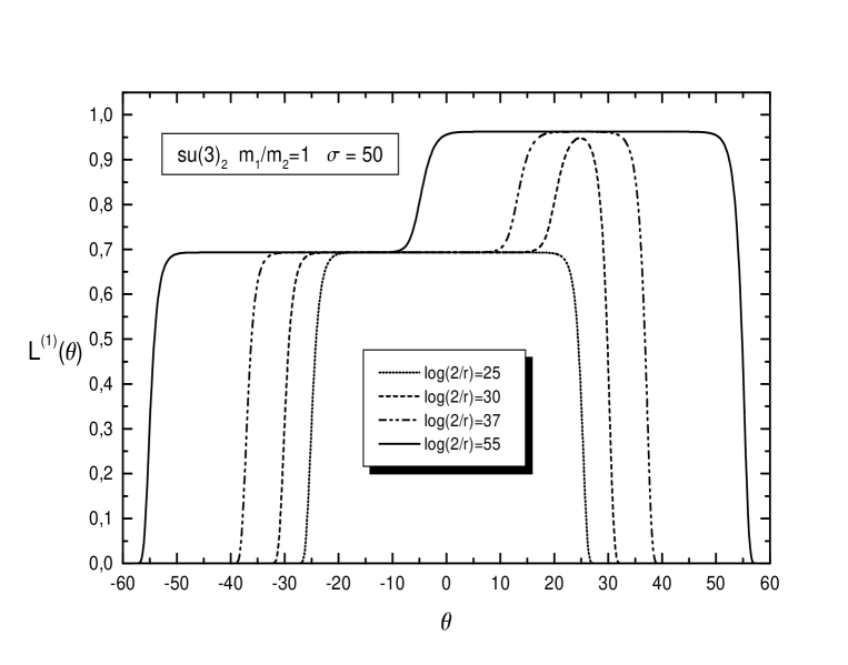
Figure 3.2: Numerical solution for ${L^{1}(\theta)}$ of the ${su(3)_{2}}$ related TBA-equations at different values of the scale parameter ${r}$ and fixed resonance shift and mass ratio.

The $Y$-systems (3.98) for $k=2$ read

$$Y_{1}^{i}\left(\theta+i\frac{\pi}{2}\right)Y_{1}^{i}\left(\theta-i\frac{\pi}{2}\right)=1+Y_{1}^{j}(\theta-\sigma_{ji})\quad i,j=1,2,\;i\neq j\,\,.$$ (3.102)

For $\sigma=0$ they coincide with the ones derived in [126] for the “massless” subsystem. Shifting the arguments in (3.102) appropriately, the periodicity

$$Y_{1}^{i}\left(\theta+\frac{5\pi i}{2}+\sigma_{ji}\right)=Y_{1}^{j}(\theta)\,\,$$ (3.103)

is obtained after a few manipulations. For a vanishing resonance parameter the relation (3.103) coincides with the one obtained in [21, 126]. These periods may be exploited in a series expansion of the scaling function in terms of the conformal dimension of the perturbing operator [21, 116]

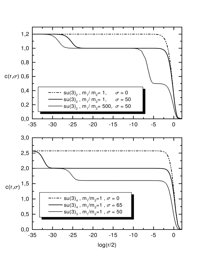
Figure 3.3: Numerical plots of the scaling function for ${su(3)_{k},\;k=2,3,4}$ as a function of the variable ${\ln(r/2)}$ at different values of the resonance shift and mass ratio.

All the results obtained in this subsection for the $SU(3)_{2}$-HSG will be reproduced in the next chapter within the context of a very different framework, the so-called form factor approach. In particular, the relation between the presence of resonance parameters in the S-matrix and the interpretation of the observed flows as massless flows will receive important support in the form factor context. Notice that in the TBA-context the conformal dimension of the perturbation can be related to the periodicities of the $Y$-systems, but such relationship is conjectured once the expected value of the conformal dimension $\Delta$ is known (see (2.121)). In the next chapter we will compute this conformal dimension in a completely different way and confirm the result conjectured in the TBA-context. In addition, we will be able to compute conformal dimensions of fields other than the one of the perturbing operator, which is up to now not possible in the TBA-approach.

3.4.2 The ${SU(3)_{3}}$-HSG model

This model consists of two pairs of solitons $\overline{(1,1)}=(2,1)$ and $\overline{(1,2)}=(2,2)$. When the soliton $(1,i)$ scatters with itself it may form $(2,i)$ for $i=1,2$ as a bound state. The two-particle S-matrix elements read

$$S^{ii}(\theta)=\left(\begin{array}[]{ll}(2)_{\theta}&-(1)_{\theta}\\ -(1)_{\theta}&(2)_{\theta}\end{array}\right)\quad\quad S^{ij}(\theta-\sigma_{ij})=\left(\begin{array}[]{ll}\eta_{ij}\,(-1)_{\theta}&\eta_{ij}^{2}\,(-2)_{\theta}\\ \eta_{ij}^{2}\,(-2)_{\theta}&\eta_{ij}\,(-1)_{\theta}\end{array}\right)\;.$$ (3.104)

Since soliton and anti-soliton of the same colour obey the same TBA equations we can exploit charge conjugation symmetry to identify $\epsilon^{i}(\theta):=\epsilon_{1}^{i}(\theta)=\epsilon_{2}^{i}(\theta)$ leading to the reduced set of equations

$$\epsilon^{i}(\theta)+\varphi*L^{i}(\theta)-\varphi*L^{j}(\theta-\sigma_{ji})=rM^{i}\cosh\theta,\quad\varphi(\theta)=-\frac{4\sqrt{3}\cosh\theta}{1+2\cosh 2\theta}\;.$$ (3.105)

The corresponding scaling function therefore acquires a factor two,

$$c(r,\sigma)=\frac{6\,r}{\pi^{2}}\sum_{i}M^{i}\int d\theta\,\cosh\theta\,L^{i}(\theta)\;.$$ (3.106)

This system exhibits remarkable symmetry properties. We consider first the situation $\sigma=0$ with $m_{1}=m_{2}$ and note that the system becomes free in this case

$$M^{1}=M^{2}=:M\;\Rightarrow\;\epsilon^{1}(\theta)=\epsilon^{2}(\theta)=rM\cosh\theta\;,$$ (3.107)

meaning that the theory falls apart into four free fermions whose central charges add up to the expected coset central charge of $2$. Also for unequal masses $m_{1}\neq m_{2}$ the system develops towards the free fermion theory for high energies, when the difference becomes negligible. This is also seen numerically.

For $\sigma\neq 0$ the two copies of the minimal $A_{2}$-ATFT or equivalently the scaling Potts model start to interact. The outcome of the TBA-analysis in that case is summarized as

Unstable particle formation $$: \text{\qquad\quad}c_{su(3)_{3}}=2=c_{UV}+\hat{c}_{UV}=\frac{6}{5}+\frac{4}{5},$$

No unstable particle formation $$: \text{\qquad\quad}2c_{su(2)_{3}}=\frac{8}{5}=c_{IR}+\hat{c}_{IR}=\frac{4}{5}+\frac{4}{5}\,\,\,.$$

As discussed in the previous case for $k=2$, the $L$-functions develop an additional plateau after passing the point $-x=\sigma/2$. This plateau lies at $L=\ln 2$ which is the free fermion value signaling that the system contains a free fermion contribution in the UV-limit as soon as the interaction between the solitons of different colours becomes relevant. Fig. 3.3 exhibits the same behaviour as the previous case. We clearly observe the plateau at $8/5$ corresponding to the two non-interacting copies of the minimal $A_{2}$-ATFT. As soon as the energy scale of the unstable particles is reached, the scaling function approaches the correct value of $c=2$.

The $Y$-systems (3.98) for $k=3$ read

$$Y_{1,2}^{i}\left(\theta+i\frac{\pi}{3}\right)Y_{1,2}^{i}\left(\theta-i\frac{\pi}{3}\right)=Y_{1,2}^{i}\left(\theta\right)\frac{1+Y_{1,2}^{j}(\theta+\sigma_{ij})}{1+Y_{1,2}^{i}\left(\theta\right)}\quad i,j=1,2,\;i\neq j\,\,.$$ (3.108)

Once again we may derive a periodicity

$$Y_{1,2}^{i}\left(\theta+2\pi i+\sigma_{ji}\right)=Y_{1,2}^{j}(\theta),$$ (3.109)

by making the suitable shifts in (3.108) and subsequent iteration.

3.4.3 The ${SU(3)_{4}}$-HSG model

This model involves 6 solitons, two of which are self-conjugate $\overline{(2,1)}=(2,1)$, $\overline{(2,2)}=(2,2)$ and two conjugate pairs $\overline{(1,1)}=(3,1)$, $\overline{(1,2)}=(3,2)$. The corresponding two-particle S-matrix elements are obtained from the general formulae (2.142) and (2.145)

$$S^{ii}(\theta)=\left(\begin{array}[]{ccc}(2)_{\theta}&(3)_{\theta}(1)_{\theta}&-(2)_{\theta}\\ (3)_{\theta}(1)_{\theta}&(2)_{\theta}^{2}&(3)_{\theta}(1)_{\theta}\\ -(2)_{\theta}&(3)_{\theta}(1)_{\theta}&(2)_{\theta}\end{array}\right),$$ (3.110)

for soliton-soliton scattering with the same colour values and

$$S^{ij}(\theta-\sigma_{ij})=\left(\begin{array}[]{ccc}\eta_{ij}(-1)_{\theta}&\eta_{ij}^{2}(-2)_{\theta}&\eta_{ij}^{3}(-3)_{\theta}\\ \eta_{ij}^{2}(-2)_{\theta}&-(-3)_{\theta}(-1)_{\theta}&\eta_{ij}^{2}(-2)_{\theta}\\ \eta_{ij}^{3}(-3)_{\theta}&\eta_{ij}^{2}(-2)_{\theta}&\eta_{ij}(-1)_{\theta}\end{array}\right),$$ (3.111)

for the scattering of solitons of different colours with $\eta_{12}=e^{i\frac{\pi}{4}}$. In this case the numerical analysis becomes more involved, but for the special case $m_{1}=m_{2}$ one can reduce the set of six coupled integral equations to only two by exploiting the symmetry $L_{a}^{1}(\theta)=L_{a}^{2}(-\theta)$ and using charge conjugation symmetry, $L_{1}^{i}(\theta)=L_{3}^{i}(\theta)$. The numerical outcomes, shown in Fig. 3.3 again match with the analytic expectations (3.84) and yield for $-x=\ln(2/r)>\sigma/2$ the coset central charge of $18/7$. In summary we obtain:

Unstable particle formation $$: \text{\qquad\quad}c_{su(3)_{4}}=\frac{18}{7}=c_{UV}+\hat{c}_{UV}=\frac{11}{7}+1$$

No unstable particle formation $$: \text{\qquad\quad}2c_{su(2)_{4}}=2=c_{IR}+\hat{c}_{IR}=1+1\,\,\,,$$

which matches precisely the numerical outcome in Fig.3.3, with the same physical interpretation as already provided in the previous two subsections.

3.4.4 The semi-classical limit ${k\rightarrow\infty}$

As last example we carry out the limit $k\rightarrow\infty$, which is of special physical interest since it may be identified with the weak coupling or equivalently the classical limit, as is seen from the relation $\hbar\beta^{2}=1/k+O(1/k^{2}).$ To illustrate this equivalence we have temporarily re-introduced Planck’s constant. It is clear from the TBA-equations that this limit may not be taken in a straightforward manner. However, we can take it in two steps, first for the on-shell energies and the kernels and finally for the sum over all particle contributions. The on-shell energies are easily computed by noting that the mass spectrum becomes equally spaced for $k\rightarrow\infty$

$$M_{a}^{i}=M_{k-a}^{i}=\frac{k}{\pi}m_{i}\sin\frac{\pi\,a}{k}\approx a\,m_{i}\;\qquad,\quad a<\frac{k}{2}\;.$$ (3.112)

For the TBA-kernels the limit may also be taken easily from their integral representations

$$\phi_{ab}(\theta)\stackunder{k\rightarrow\infty}{\longrightarrow}2\pi\,\delta(\theta)\,\left(\delta_{ab}-2\left(K^{A_{k-1}}\right)_{\,\,\,ab}^{-1}\right)$$

$$\psi_{ab}(\theta)\stackunder{k\rightarrow\infty}{\longrightarrow}2\pi\,\delta(\theta)\,\left(K^{A_{k-1}}\right)_{\,\,\,ab}^{-1},\;$$ (3.113)

when employing the usual integral representation of the delta-function. Inserting these quantities into the TBA-equations yields

$$\epsilon_{a}^{i}(\theta)\approx r\,a\,m_{i}\cosh\theta-\sum_{b=1}^{k-1}\left(\delta_{ab}-2\left(K^{A_{k-1}}\right)_{\,\,\,ab}^{-1}\right)L_{b}^{i}(\theta)-\sum_{b=1}^{k-1}\left(K^{A_{k-1}}\right)_{\,\,\,ab}^{-1}L_{b}^{j}(\theta-\sigma)\;.$$ (3.114)

We now have to solve these equations for the pseudo-energies. In principle we could proceed in the same way as in the case for finite $k$ by doing the appropriate shifts in the rapidity. However, we will be content here to discuss the cases $\sigma\rightarrow 0$ and $\sigma\rightarrow\infty$, which, as follows from our previous discussion, correspond to the situation of restored parity invariance and two non-interacting copies of the minimal ATFT, respectively. The related solutions to the constant TBA-equations (3.73) and (3.76) become

$$\sigma\rightarrow\infty:\;\hat{x}_{a}\stackunder{k\rightarrow\infty}{\longrightarrow}\frac{(a+1)^{2}}{a(a+2)}-1\quad\text{and\quad}\sigma\rightarrow 0:\;x_{a}\stackunder{k\rightarrow\infty}{\longrightarrow}\frac{(a+1)(a+2)}{a(a+3)}-1\;.$$ (3.115)

The other information we may exploit about the solutions of (3.114) is that for large rapidities they tend asymptotically to the free solution, meaning that

$$\sigma\rightarrow 0,\infty\;:\;\;\;\;\;L_{a}^{i}(\theta)\stackunder{\theta\rightarrow\pm\infty}{\longrightarrow}\ln(1+e^{-r\,a\,m_{i}\cosh\theta}).$$ (3.116)

We are left with the task to seek functions which interpolate between the properties (3.115) and (3.116). Inspired by the analysis in [143] we take these functions to be

$$\sigma \rightarrow \infty\;:\;\;\;\;\;L_{a}^{i}(\theta)=\ln\left[\frac{\sinh^{2}\left(\frac{a+1}{2}\,rm_{i}\cosh\theta\right)}{\sinh\left(\frac{a\,}{2}\,rm_{i}\cosh\theta\right)\sinh\left(\frac{a+2}{2}\,rm_{i}\cosh\theta\right)}\right],\,\,\,$$ (3.117)

$$\sigma \rightarrow 0\;:\;\;\;\;\;L_{a}^{i}(\theta)=\ln\left[\frac{\sinh\left(\frac{a+1}{2}\,rm_{i}\cosh\theta\right)\sinh\left(\frac{a+2}{2}\,rm_{i}\cosh\theta\right)}{\sinh\left(\frac{a}{2}\,rm_{i}\cosh\theta\right)\sinh\left(\frac{a+3}{2}\,rm_{i}\cosh\theta\right)}\right].\,\,\,$$ (3.118)

The expression (3.117) coincides with the expressions discussed in the context of the breather spectrum of the sine-Gordon model [143] and (3.118) is constructed in analogy. We are now equipped to compute the scaling function in the limit $k\rightarrow\infty$

$$c(r,\sigma)=\lim_{k\rightarrow\infty}\frac{3\,r}{\pi^{2}}\sum_{i=1}^{2}\int d\theta\,\cosh\theta\sum_{a=1}^{k-1}M_{a}^{i}L_{a}^{i}(\theta)\,\,.$$ (3.119)

Using (3.112), (3.117) and (3.118) the sum over the main quantum number may be computed directly by expanding the logarithm. We obtain for $k\rightarrow\infty$

$$\lim_{\sigma\rightarrow\infty}c(r) = -\dfrac{6r}{\pi^{2}}\,\,\sum_{i=1}^{2}\!\!\int\,\,d\theta\,m_{i}\cosh\theta\ln\left(1-e^{-r\,m_{i}\cosh\theta}\right),$$ (3.120)

$$\lim_{\sigma\rightarrow 0}c(r) = -\dfrac{6\,r}{\pi^{2}}\,\,\sum_{i=1}^{2}\!\!\int\!\!d\theta\,\,m_{i}\cosh\theta[\ln\left(1-e^{-r\,m_{i}\cosh\theta}\right)+$$ (3.121)

$$+ \,\,\,\,\,\,\,\,\ln(1-e^{-r\,2m_{i}\cosh\theta})].\,$$

Here we have acquired an additional factor of 2, resulting from the identification of particles and anti-particles which is needed when one linearizes the masses in (3.112). Taking now the limit $r\rightarrow 0$ we obtain

no unstable particle formation $$: \text{\quad\ }2\,c_{su(2)_{\infty}}=4\;$$ (3.122)

unstable particle formation $$: \text{\quad\ }c_{su(3)_{\infty}}=6\,\,.$$ (3.123)

The results (3.120), (3.122) and (3.121), (3.123) allow a nice physical interpretation. We notice that for the case $\sigma\rightarrow\infty$ we obtain four times the scaling function of a free boson. This means in the classical limit we obtain twice the contribution of the non-interacting copies of $SU(2)_{\infty}/U(1)$, whose particle content reduces to two free bosons each of them contributing $1$ to the effective central charge which is in agreement with (2.123). For the case $\sigma\rightarrow 0$ we obtain the same contribution, but in addition the one from the unstable particles, which are two free bosons of mass $2m_{i}$. This is also in agreement with (2.123).

Finally, it is interesting to observe that, when taking the resonance poles to be $\theta_{R}=\sigma-i\pi/k$, the semi-classical limit taken in the Breit-Wigner formula (2.102) leads to $m_{\tilde{k}}^{2}=(m_{i}+m_{j})^{2}$. On the other hand (3.121) seems to suggest that $m_{\tilde{k}}=2m_{i}$, which implies that the mass scales should be the same. However, since our analysis is mainly based on exploiting the asymptotics we have to be cautious about this conclusion.

3.5 Summary of results and open points

Our main conclusion is that the TBA-analysis indeed confirms the consistency of the scattering matrix proposed in [51]. In the deep ultraviolet limit we recover the $G_{k}/U(1)^{\ell}$-coset central charge for any value of the $2\ell-1$ free parameters entering the S-matrix, including the choice when the resonance parameters vanish and parity invariance is restored on the level of the TBA-equations. This is in contrast to the properties of the S-matrix, which is still not parity invariant due to the occurrence of the phase factors $\eta$, which are required to close the bootstrap equations [51]. However, they do not contribute to the TBA-analysis, which means that so far we can not make any definite statement concerning the necessity of the parity breaking, since the same value for the central charge is recovered irrespective of the value of the $\sigma$’s. The underlying physical behaviour is, however, quite different as our numerical analysis demonstrates:

• For vanishing resonance parameter $\sigma=0$ and taking the energy scale of the stable particles to be of the same order $m_{1}\simeq m_{2}$, the deep ultraviolet coset central charge is reached straight away. From the physical point of view, this is the expected behaviour since, according to (2.103) whenever the resonance parameter is vanishing the same happens to the decay width of the unstable particles. Therefore, the unstable particles become “virtual states” characterised by poles in the imaginary axis, beyond the physical sheet. They are on an energy scale of the same order as the one of the stable particles. Being the energy scale corresponding to the onset of all stable and unstable particles of the same order, the scaling function takes the value corresponding to the ultraviolet coset central charge of the underlying CFT as soon as the mentioned scale is reached. As shown in section 3.3.3, for $\sigma=0$ and $m_{1}=m_{2}$ parity is restored at the level of the TBA-equations and consequently the corresponding $L$-functions must be symmetric in the rapidity variable. Although no numerical results are presented which confirm this statement it is clear from Fig. 3.2 that the $L$-functions cease to be symmetric as soon as parity invariance is violated.

• On the other hand, for non-trivial resonance parameter, the scaling function passes the different regions in the energy scale. It develops then a “staircase” behaviour where the number and size of the plateaux is determined by the relative mass scales between the stable and unstable particles and the stable particles themselves. Therefore, different choices of the $2\ell-1$ free parameters at hand lead to a theory with a different physical content, but still possessing the same central charge. This feature is also consistent with the physical picture anticipated for the HSG-models, since in the deep ultraviolet limit, as long as the resonance parameter is finite, the energy scale is much higher than the energy scales necessary for the production of all the stable and unstable particles. Therefore all the particle content of the model contributes to the scaling function which, interpreted as a measure of effective light degrees of freedom, will reach its maximum value, namely the Virasoro central charge of the unperturbed CFT. Being parity broken through the resonance shift $\sigma$, the $L$-functions cease to be symmetric as soon as the energy scale of the unstable particles is reached and develop also plateaux as shown in Fig. 3.2.

  It must be emphasised that the sort of flows observed correspond to a system of TBA-equations which formally, after the introduction of the auxiliary parameter $r^{\prime}=r/2\,e^{\sigma/2}$, can be re-interpreted as the TBA-equations corresponding to two massless systems, in the spirit of [126]. As we have mentioned, the connection between flows related to the presence of unstable particles in the spectrum and massless flows should be understood as formal at this point, since the parameter $r^{\prime}$ was only introduced aiming towards a simplification of the analytical and numerical analysis. However, in the two subsequent chapters we will collect additional arguments which support the belief that the observed flows should be in fact understood as effective massless flows.

The similar “staircase” behaviour observed both for the HSG-models and for the models studied in [108, 109, 110] has been emphasised in several occasions along this chapter. Therefore, it is appropriate at this point to clarify our understanding about the origin of this similarity. The presence of resonance poles in the spectrum is characteristic of both sorts of theories but, as we will justify now, the “staircase” behaviour of the scaling function does not admit the same clear physical interpretation for the models studied in [108, 109, 110] than for the HSG-models.

Whereas for the HSG-models the resonance parameter enters the S-matrix as a shift in the rapidity variable, in the models studied in [108, 109, 110], the resonance parameter arises as a consequence of the analytical continuation to the complex plane of the effective coupling constant $B$, which characterises the Lagrangian and S-matrix of the sinh-Gordon model [43] and, in fact, of all affine Toda field theories related to simply-laced Lie algebras [35, 36, 37]. The mentioned complexification takes place in the following way

$$B\rightarrow 1\pm\frac{2i\sigma}{\pi}.$$ (3.124)

It is interesting to notice that the particular form of (3.124) is not casual. In particular, the real part of $B$ has necessarily to be one so that the consequent transformation of the sinh-Gordon S-matrix via (3.124) generates a new but still consistent S-matrix, in the sense described in section 2.3 of the preceding chapter. The consistency of the new S-matrix in guaranteed by the fact that, for all affine Toda field theories [35, 36], the coupling constant $B$ occurs always in the combination $B(2-B)$, which stays real under (3.124). $B=1$ is the so-called self-dual point since in that case $B=2-B$.

The introduction of the resonance parameter $\sigma$ by means of (3.124) makes the S-matrix exhibit a resonance pole in the imaginary axis $\theta_{R}=-\sigma-\frac{i\pi}{2}$ similarly to the $SU(3)_{2}$-HSG model. As usual this pole could be understood as the trace of an unstable particle. However, even though only one resonance parameter has been introduced, the TBA-analysis carried out in [108] for the roaming sinh-Gordon model shows that the corresponding scaling function develops an infinite number of plateaux. Therefore, the results in [108] can not be interpreted physically by using the same sort of arguments employed in the TBA-analysis of the HSG-models. Equivalently, the infinite number of plateaux observed in [108] can not be related to the number of free parameters in the model. The same can be said with respect to the models studied in [109, 110] whose construction follows the same lines, i.e. performing the transformation (3.124) introduced for the roaming sinh-Gordon model, with the difference that they take as an input the S-matrices of other simply laced affine Toda field theories instead of the sinh-Gordon model ($A_{1}^{(1)}$-ATFT), which is the simplest of their class.

Although all the results of this chapter confirm the consistency of the S-matrix proposal [51] there are important data concerning the underlying CFT which have not been reproduced in the TBA-context. For instance, it would be highly desirable to carry out the series expansion (3.99) of the scaling function in $r$ and determine the dimension $\Delta$ of the perturbing operator. It will be useful for this to know the periodicities of the $Y$-functions. In the light of the results found in section 3.4 and the expected value of $\Delta$ given by (2.121), we conjecture that they will be

$$Y_{a}^{i}\left(\theta+i\pi(1-\Delta)^{-1}+\sigma_{ji}\right)=Y_{\bar{a}}^{j}(\theta).$$ (3.125)

For vanishing resonance parameter and the choice $g=su(2)$, this behaviour coincides with the one obtained in [139]. This suggests the form in (3.125) is of a very universal nature beyond the models discussed here and supports our conjecture. It would be highly desirable to have a model-independent explanation for this behaviour starting from first principles.

Thus, concerning the issue of the identification of the conformal dimension of the perturbing operator we have to conclude that, although the preceding arguments support the conjecture (3.125), more work and/or different tools are needed in order to make a definite statement. However, one should also keep in mind that the perturbing operator, although playing a distinguished role in the construction of the massive QFT, does not of course fulfill all the operator content of the underlying CFT. The latter operator content is well known for the WZNW-coset theories [59, 61]. In particular, the corresponding conformal dimensions can be obtained easily by means of a general formula which might be found also in [59, 61]. Unfortunately, the question of how to identify the whole operator content of the underlying CFT is left unanswered in the TBA-framework and we must appeal to a different method if we intend to really fulfill all the relevant data, apart from (2.121) and (2.123), characterising the ultraviolet CFT. A different approach which allows to find an answer to the latter question and provides at the same time all the information extracted from the preceding TBA-analysis shall be presented in the two succeeding chapters. The mentioned approach is the so-called form factor program originally pioneered by the members of the Berlin group M. Karowski and P. Weisz in [22]. Apart from providing a consistency check, in comparison with the TBA-analysis, this approach also serves to develop the theory further towards a full-fledged QFT.

We also observe from our $su(N)$-example that the two regions, $k>h$ for which quantum integrability was explicitly shown in [48], and $k\leq h$, for which quantum integrability has not been established up to now, do not show up in our analysis. As we mentioned at the beginning of section 3.4, this might be due to the fact that the constraint $k>h$ arises when we select out those models which are super-renormalisable at first order (see definition in subsection 2.1.2). For these models the task of explicitly constructing quantum conserved charges gets simplified as shown in [18] (see also subsection 2.1.2). However, there is no reason why the HSG-models which are no super-renormalisable at first other should not be integrable. Therefore, the results emerging from our TBA-analysis are not contradictory and could be understood as an indication of the fact that possibly all HSG-models, irrespectively of the value of the level $k$, are quantum integrable. In order to check the previous conjecture, it would be desirable to explicitly construct quantum conserved charges associated to the HSG-models corresponding also to $k<h$, or prove their integrability by other means like, for instance, the ‘counting-argument’ reported in subsection 2.1.2.

It would be very interesting to extend the case-by-case analysis of section 3.4 to other algebras. The first challenge in these cases is to incorporate the different resonance parameters, namely increase the rank of the Lie algebra. However, it is clear from our analysis that the number of TBA-equations to be solved increases precisely with the rank of the Lie algebra. This means that a TBA-analysis will become very complicate as soon as $\ell>2$, both from the analytical and numerical point of view. Concerning this problem, although having also its particular inconveniences for high rank, the form factor program mentioned above is more advantageous (see chapter 5).

Chapter 4 Form Factors of the Homogeneous sine-Gordon models.

A form factor in QFT is a matrix element of a local operator between the vacuum state and an $n$-particle $in$-state. Despite the fact that we will focus our attention on the properties and applications of form factors within the context of integrable massive 1+1-dimensional QFT’s, they are objects which have been analysed in the framework of 1+3-dimensional QFT’s over the last 40 years. In the latter context, they are frequently introduced as functions characterising the scattering amplitude associated to the interaction of a charged particle with an external electromagnetic field or the electromagnetic field of another particle (see e.g. [144, 15]). However, the form factor approach was not exploited in the context of 1+1-dimensional QFT’s until 1977, when the pioneering work due to P. Weisz and M. Karowski [22] was published. In these seminal papers, the fundamental properties of form factors in 1+1-dimensional theories were established. It was found that, similarly to the construction procedure of S-matrices for integrable massive 1+1-dimensional QFT’s described in chapter 2, the form factors associated to a certain operator can be obtained as the solutions to a set of consistency equations whose origin is based on physically-motivated requirements. It is also in 1+1-dimensions when the form factor approach turns out to be most powerful for various reasons. First, the solution to the mentioned consistency equations allows in principle for computing all $n$-particle form factors associated to any local field of the massive QFT. Also, once the form factors associated to certain local operators of the QFT are known, they might be used for many interesting applications like computing correlation functions, determining the operator content of the perturbed CFT or explicitly compute other relevant quantities which characterise the underlying CFT.

After the original papers [22], the development of the form factor approach in the context of 1+1-dimensional integrable QFT’s has been carried out to a large extent by F.A. Smirnov et al. [145, 160, 153]. However, the interest of this approach within the context of 1+1-dimensional QFT’s constructed as perturbed CFT’s received renewed interest with the work of J.L. Cardy and G. Mussardo [156, 157]. After that, the form factor program has been carried out for different models, under several different aspects and by many authors. Some of these works are [152, 154, 155, 157, 158, 159, 161, 27, 162]. The latter list is not meant to be complete.

Concerning the present status of the form factor approach, there are still a lot of open problems some of which we itemize below, mentioning also the particular contributions of our work to their understanding.

Reviewing the present status of the form factor approach

Generic building blocks

Although the form factors are obtained as the solutions to a certain set of consistency equations which we will see in detail later, it is not known by now whether there exist or not general ‘building blocks’ in terms of which any form factor of a 1+1-dimensional integrable and massive QFT can be expressed, similarly to the situation encountered in the construction of exact S-matrices along the lines of subsection 2.3. There are various places in the literature [158, 159, 152] were determinant expressions in terms of elementary symmetric polynomials depending upon the particle rapidities have been found for the form factors associated to certain operators. This is also the case for a large class of local operators of the $SU(N)_{2}$-HSG models we have studied here. As we will see later, these determinant expressions can be equivalently written in terms of contour integrals and various types of integral representations can be found in the literature whose precise inter-relation still needs to be clarified. Once the building blocks are known one may pose the question how are they combined by means of Lie algebraic quantities, analogously to the S-matrix construction (see [39, 40, 41]).

Closed solutions

However, the open questions stated in the previous paragraph go already beyond the present status of understanding of the form factor approach for many models, meaning that, the questions pointed out above, may be posed once all $n$-particle form factors associated to a certain operator of the QFT have been constructed. This is not the usual case and, from that point of view, the situation we will encounter in the course of our precise analysis is quite extraordinary, since we will find close formulae for all $n$-particle form factors related to a large class of operators. Therefore, it is still an open problem how to solve in general all the consistency equations any form factor of a 1+1-dimensional QFT has to satisfy. For many models only the form factors associated to the lowest values of $n$ and/or to specific local operators of the theory have been constructed.

Identification of the operator content

Similarly again to the situation arising in the construction of S-matrices, where specific information about the theory under consideration only enters at quite a late stage of the construction, several of the consistency equations satisfied by form factors do not require any knowledge about the precise nature of the local operator at hand. Therefore, once a solution is found one still needs to identify the precise operator it corresponds to. There are various constraints which can be used in order to match each form factor solution with a concrete operator of the massive QFT but still, the techniques available need to be refined, since there is no systematic way to identify all local operators of the QFT, as we may find in the context of our precise analysis.

Ultraviolet limit

Concerning the identification of operators mentioned in the previous point, one of the open problems which is worth mentioning here is the fact that such an identification is ultimately performed by assuming a one-to-one correspondence between the operator contents of the perturbed and unperturbed CFT, for the primary field content. Provided the latter is known (which is not always the case) one can use various techniques to identify the ultraviolet conformal dimensions of the local fields of the massive QFT by exploiting the knowledge of their form factors. However, these techniques still need also refinement, since they do not allow for unraveling the possible degeneracy of the operators of the underlying CFT and sometimes they can not be used for all operators, or they do not allow for a clear-cut identification of the ultraviolet conformal dimension. This means that having a priori a relatively good guess for its value turns out to be very important.

Two-point correlation functions

As mentioned above, one of the most important objects one is in principle in the position to compute once the form factors of certain operators are known is any two-point correlation function involving these operators. It can be proven that these two-point functions admit an expression in terms of an infinite series where the $n$-th term is an $n$-dimensional integral in the rapidities whose integrand depends on the $n$-particle form factors of the two operators arising in the correlation function. Concerning the computation of correlation functions in the form factor context i.e., the evaluation of the aforementioned series, there are aspects which need further investigation. First, it is not known up to now any rigorous proof of the convergence of the series mentioned above, which is generally assumed in the light of the behaviour observed for several models. Second, the evaluation of the multi-dimensional integrals arising in this series requires a lot of computer time already for $n\geq 6$, which means it would be very interesting to investigate whether it is possible to sum the mentioned series analytically.

Momentum space cluster property

Finally, we would like to briefly mention that some of the general properties of form factors still lack a rigorous proof for the time being. One of them is the momentum space cluster property, whose investigation for the $SU(3)_{2}$-HSG model will provide, in our opinion, a valuable contribution to the present status of understanding of this characteristic of form factors, which has been observed for several concrete models in the literature [164, 152, 159, 165].

Locality

Another property which needs further investigation is the locality of the operators arising in the form factor definition, which is a fundamental requirement one should be able to prove in the form factor framework in order to definitely confirm that the objects we want to construct characterise a properly defined QFT. We will mention later that some attempts for such a proof may be found in the literature but they all hold only for particular types of QFT’s and operators.

Main purposes of the form factor analysis

In the light of the previous historical review and summary of open questions we can already anticipate the main purposes our form factor analysis will serve for:

i) Develop further the QFT associated to the HSG-models.

ii) After the physical picture emerging from [49, 50] and [51] has been confirmed by the thermodynamic Bethe ansatz analysis of the preceding chapter [20, 21], the form factor analysis may be exploited as an alternative approach which allows for double-check and even go beyond the TBA-results, providing in this way also a more exhaustive check for the consistency of the S-matrix proposal [51], i.e. more information about the underlying CFT.

iii) Apart from the two preceding points, which explicitly point out the utilisation of the form factor approach as a means for extracting information characteristic from the specific models at hand, our concrete form factor analysis will also provide a valuable contribution to the understanding of various properties and applications of form factors which, in the light of the previous historical introduction, need further clarification. We will specify in more detail later the concrete contributions of our work in this direction.

Recall that the main outcome of our TBA-analysis has been the identification of the Virasoro central charge of the underlying CFT and the numerical computation of the finite size scaling function [21, 116] for which a “staircase” pattern intimately related to the presence of unstable particles in the spectrum [89, 14, 51] and indicating the different energy scales of unstable and stable particles, has been observed. Also the conformal dimension of the perturbing operator emerged in the context of the TBA by conjecturing a relationship between the latter quantity and the periodicities of the so-called $Y$-systems [139].

However, at present we know that the identification of the operator content of a 1+1-dimensional QFT starting from its scattering theory is not achievable in the TBA-context (apart from the possible identification of the conformal dimension of the perturbing operator outlined above) and in fact, for general quantum field theories is still an outstanding issue whose investigation has great interest in its own right.

It is worth mentioning that recently a link between scattering theory and local interacting fields in terms of polarisation-free generators has been developed [146, 147]. Unfortunately, they involve subtle domain properties and are therefore objects which concretely can only be handled with great difficulties. On the other hand, the central concepts of relativistic quantum field theory, like Einstein causality and Poincaré covariance, are captured in local field equations and commutation relations. As a matter of fact local quantum physics (algebraic quantum field theory) [148] takes the collection of all operators localised in a particular region, which generate a von Neumann algebra, as its very starting point (for recent reviews see e.g. [149, 150]). Ignoring subtleties of non-asymptotic states, it is essentially possible to obtain the latter picture from the former, namely the “particle picture”, by means of the LSZ-reduction formalism [151].

Fortunately, in the context of 1+1-dimensional QFT’s, the form factor approach [22] turns out to be very convenient for the purposes summarised two paragraphs ago. As was said before, form factors are matrix elements (see Eq. (4.1)) of a certain local operator associated to a 1+1-dimensional QFT between a multi-particle in-state and the vacuum. These matrix elements can be obtained as the solutions to a certain set of consistency equations [22, 153, 152, 154, 155] which have their origin on very general principles of quantum field theory and therefore do not rely on the specific nature of the corresponding local operator. Notice that, this is very similar to the situation arising in the construction of the two-particle S-matrices related to integrable massive bi-dimensional QFT’s described in chapter 2, in the sense that the bootstrap program [12] also allows for the exact construction of these amplitudes by viewing then as the solutions to a set of consistency equations based on physical requirements such as unitarity, crossing symmetry, Hermitian analyticity or Lorentz invariance.

Once a solution for these consistency equations is found, it is left the task of relating it to a particular local operator. First of all, one shall make the assumption dating back to the initial papers [22], that each solution to the form factor consistency equations [22, 153, 152, 154, 155] corresponds to a particular local operator. Based on this, numerous authors [22, 153, 152, 155, 157, 158, 159, 160, 161, 27] have used various ways to identify and constrain the specific nature of the operator, e.g. by looking at asymptotic behaviours, performing perturbation theory, taking symmetries into account, formulating quantum equations of motion, etc. Our analysis will especially exploit the conjecture that each local operator related to a primary field has a counterpart in the ultraviolet conformal field theory.

Having identified the operator content (or at least, part of it) by means of any of the methods just summarised, the knowledge of the form factors associated to certain local operators allows immediately for the computation of correlation functions involving these operators, at least up to a certain approximation. Such a relationship can be exploited for various applications like, for instance:

i) the calculation of the two-point function of the trace of the energy momentum tensor $\Theta$, an operator whose existence in guaranteed for any QFT. Once the two-point function of the trace of energy momentum tensor is known it is possible to evaluate, usually numerically, Zamolodchikov’s $c$-function [24]. The $c$-function contains the same physical information as the finite size scaling function of the TBA, namely, in the UV-limit reduces to the Virasoro central charge of the underlying CFT whence following its renormalisation group (RG) flow we will observe the familiar “staircase” behaviour as a sign of the different mass scales of unstable and stable particles. The latter behaviour supports the interpretation of Zamolodchikov’s $c$-function as a measure of massless effective degrees of freedom in the Hilbert space. Also, by looking at the asymptotic UV-behaviour of the two-point function, it is possible to extract the conformal dimension of the perturbing operator by means of the well-known proportionality between the perturbing field and the trace of the energy momentum tensor established in [163] (see also [4]). Therefore, having determined the form factors of the trace of the energy momentum tensor, one is in principle in the position to obtain essentially all the information provided by the preceding TBA-analysis.

ii) the calculation of the two-point function of any other local operator for which the form factors are known. The latter application of form factors, allows for the possibility to study the ultraviolet behaviour of these two-point functions and determine thereafter the ultraviolet conformal dimension of the operator, namely the conformal dimension of the operator of the underlying CFT which acts as counterpart of the one under inquiry in the UV-limit. In some cases, depending on the particular internal symmetries of the model at hand, the ultraviolet conformal dimension can be also computed by means of the so-called $\Delta$-sum rule derived by G. Delfino, P. Simonetti and J.L. Cardy in [27], provided the correlation function of the operator at hand with the trace of the energy momentum tensor is known. One might also perform a renormalisation group analysis for the conformal dimensions obtained through the $\Delta$-sum rule [27] and observe the flow of the operator content from a CFT to another as the RG-parameter varies.

The concrete analysis we present in this chapter collects the results reported in [72, 73, 28] (see also [71]), and can be summarised as follows:

In this chapter we study a concrete model, the $SU(3)_{2}$-HSG model, within the form factor context. As mentioned above, form factors are solutions to a set of general consistency equations [22, 153, 152, 154, 155]. These equations are reported in section 4.1, together with a summary of the key steps involved in their solution (subsection 4.1.2) and several applications of form factors: the evaluation of correlation functions (subsection 4.1.3) and the numerical methods employed for this purpose (subsection 4.1.4), the computation of the Virasoro central charge of the underlying CFT (subsection 4.1.5), the re-construction of the operator content of the underlying CFT (subsection 4.1.6) or the development of a renormalisation group analysis which might confirm and go beyond the physical picture emerging from the TBA-analysis (subsections 4.1.7 and 4.1.8). After the general equations to be solved have been introduced, we come in section 4.2 to the description of the main features of the $SU(3)_{2}$-HSG model, emphasising especially those characteristics which may be more relevant in the form factor context. In section 4.3 we present a general ansatz for the solutions to the consistency equations summarised in section 4.1.

This ansatz depends upon certain functions which are known in the literature as minimal form factors. We recall their main properties and derive their explicit form for the model at hand. In section 4.4 we systematically construct all $n$-particle form factors associated to a large class of local operators of the $SU(3)_{2}$-HSG model. These solutions are given in terms of building blocks consisting out of determinants of matrices whose entries are elementary symmetric polynomials on the rapidities. They also admit an alternative representation in terms of contour integrals which we also present in the same section. However, at this stage of our investigation we do not provide a rigorous proof of the proposed solutions which are based on the extrapolation of the results obtained up to a certain value of $n$. In section 4.5 we illustrate the results of the previous section by particularising the form factor solutions for three concrete local operators of the theory. In section 4.6 we carry out a rigorous proof, based on very simple properties of determinants, of the solutions proposed in the preceding sections. We demonstrate how these general solutions are interrelated by the so-called momentum space cluster property in section 4.7. In particular we show that the cluster property serves also as a construction principle, in the sense that from one solution to the consistency equations we may obtain a large class, almost all, of new solutions. Having now a large set of solutions for different operators available we might exploit the knowledge of the form factors for the various applications reported in section 4.1. First of all, in section 4.8 we compute the Virasoro central charge of the underlying CFT by means of Zamolodchikov’s $c$-theorem [24]. Taking furthermore into account that the $SU(3)_{2}$-HSG model, like numerous other 1+1 dimensional integrable models, may be viewed as a perturbed CFT whose entire field content is well classified and assuming now a one-to-one correspondence between operators in the conformal and in the perturbed theory, we carry out an identification on this level that is, we identify each solution of the form factor consistency equations with a local operator which is labeled according to the ultraviolet CFT. We present this analysis in section 4.9 where we determine the ultraviolet conformal dimensions of all the operators whose form factors were constructed before. In particular, due to the outlined proportionality between the perturbing field and the trace of the energy momentum tensor [163], the latter analysis makes it possible to identify the conformal dimension of the perturbation. In section 4.10 we compute numerically the RG-flow of Zamolodchikov’s $c$-function [24] and also extend our RG-analysis to the conformal dimensions of those local operators for which the $\Delta$-sum rule [27] holds. We verify that the RG-analysis leads to a physical picture which is entirely consistent with the TBA-results and goes beyond them at the same time. Finally we review the main outcome of our analysis and point out some open problems in section 4.11.

4.1 Generalities on form factors

Before the analysis of the specific results obtained for the $SU(3)_{2}$-HSG model is presented, we must recall the definition and general properties of form factors. These properties, can be rigorously justified in most cases in terms of general principles of quantum field theory and analytic properties in the complex plane. Here we only pretend to provide a general overview of all of them in order to make comprehensible our specific study. For a more detailed derivation we refer the reader to the seminal papers [22] and specially to the book [153]. A fairly detailed review of these properties may be also found in the papers [152, 154, 155], where the form factor approach is exploited for the study of concrete models. We also make use of this section to set up the general framework and notation we shall continuously appeal to in subsequent sections.

4.1.1 The form factor consistency equations

Form factors are tensor valued functions, representing matrix elements of some local operator $\mathcal{O}({x})$ located at the origin between a multi-particle in-state and the vacuum

$$F_{n}^{\mathcal{O}|\mu_{1}\ldots\mu_{n}}(\theta_{1},\ldots,\theta_{n}):=\left\langle 0|\mathcal{O}(0)|V_{\mu_{1}}(\theta_{1})V_{\mu_{2}}(\theta_{2})\ldots V_{\mu_{n}}(\theta_{n})\right\rangle_{\text{in}}\,\,.$$ (4.1)

Recall that the vertex operators $V_{\mu_{i}}(\theta_{i})$ have been introduced in subsection 2.2.1 as a means for representing the asymptotic particle states of the QFT. Form factors, have the following general properties:

Property 1: CPT invariance

As a consequence of CPT-invariance or the braiding of two operators $V_{\mu_{i}}(\theta_{i}),V_{\mu_{i+1}}(\theta_{i+1})$ given by (2.59), one obtains

$$F_{n}^{\mathcal{O}|\ldots\mu_{i}\mu_{i+1}\ldots}(\ldots,\theta_{i},\theta_{i+1},\ldots)=F_{n}^{\mathcal{O}|\ldots\mu_{i+1}\mu_{i}\ldots}(\ldots,\theta_{i+1},\theta_{i},\ldots)S_{\mu_{i}\mu_{i+1}}(\theta_{i,i+1})\,.$$ (4.2)

Property 2: monodromy

The analytic continuation in the complex $\theta$-plane at the cuts when $\theta=2\pi i$ together with the property of crossing of the S-matrix (see Eq. (2.92) in chapter 2) lead to

$$F_{n}^{\mathcal{O}|\mu_{1}\ldots\mu_{n}}(\theta_{1}+2\pi i,\ldots,\theta_{n}) = \omega\,F_{n}^{\mathcal{O}|\mu_{2}\ldots\mu_{n}\mu_{1}}(\theta_{2},\ldots,\theta_{n},\theta_{1})=$$ (4.3)

$$= \omega\,{\prod_{i=2}^{n}}S_{\mu_{i}\mu_{1}}(\theta_{i1})\,F_{n}^{\mathcal{O}|\mu_{1}\ldots\mu_{n}}(\theta_{1},\ldots,\theta_{n}),$$

where $\omega$ is the so-called factor of local commutativity originally introduced in [154]. The meaning of such parameter as well as the motivation for its introduction will be given a bit later, when introducing the so-called ‘kinematical residue equation’.

The former two properties are usually referred to as Watson’s equations [166].

The pole structure of the form factors is encoded in the two following properties (3 and 4) which have the form of recursive equations relating form factors associated to different numbers of particles. For reasons which become clear below, such pole structure is fundamental in order to find explicit solutions to the form factor consistency equations.

Property 3: kinematical residue equation

The first type of simple poles arise for a form factor whose first two particles are conjugate to each other. In that case we have a kinematical pole at $\theta=i\pi$, $\theta$ being the rapidity difference between these two particles. The existence of this simple pole leads to a recursive equation relating the $(n+2)$- and the $n$-particle form factor

$$\stackunder{{\small\bar{\theta}}_{0}\rightarrow{\small\theta}_{0}}{\text{Res}}{\small F}_{n+2}^{\mathcal{O}|\bar{\mu}\mu\mu_{1}\ldots\mu_{n}}{\small(\bar{\theta}}_{0}{\small+i\pi,\theta}_{0}{\small,\theta}_{1}{\small,\ldots,\theta}_{n}{\small)}=i(1-\omega\prod_{l=1}^{n}S_{\mu\mu_{l}}(\theta_{0l})){\small F}_{n}^{\mathcal{O}|\mu_{1}\ldots\mu_{n}}{\small(\theta}_{1}{\small,\ldots,\theta}_{n}{\small),}$$ (4.4)

with $\omega$ being the so-called factor of local commutativity and $\bar{\mu}$ the anti-particle of $\mu$ (see Fig. 4.1).

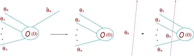
Figure 4.1: Kinematical pole residue equation for form factors: ${F_{n+2}^{\mathcal{O}}\rightarrow F_{n}^{\mathcal{O}}}$.

Property 4: bound state residue equation

The second type of simple poles we referred to occur only when bound states are present in the model. When this happens, the corresponding form factors have poles located at the values of the rapidity in the physical strip $0\leq\text{Im}(\theta)\leq\pi$ corresponding to fusing angles of the S-matrix (see section 2.3 in chapter 2). This gives rise to another set of recursive equations relating now the $(n+1)$- and the $n$-particle form factor.

Recall that if two particles $A,B$ interact to form a stable bound state ${C}$ i.e, $A+B\rightarrow{C}$, there is a pole in the corresponding two particle amplitude at $\theta_{AB}=iu_{AB}^{C}$ of the form

$$\stackunder{{\small\theta}\rightarrow{\small i(\pi-u_{AB}^{C})}}{\text{Res}}S_{AB}(\theta)=i(\Gamma_{AB}^{C})^{2},$$ (4.5)

where $\Gamma_{AB}^{C}$ is the three-particle vertex on mass-shell and we are always assuming the S-matrix to be diagonal. The corresponding residue equation for the form factors is given by [167]

$$\lim_{\epsilon\rightarrow 0}\epsilon\,F_{n+1}^{\mathcal{O}|A\,B\mu_{1}\ldots\mu_{n-1}}(\theta+i\bar{u}_{AC}^{B}-\epsilon,\theta-i\bar{u}_{BC}^{A}+\epsilon,\theta_{1},\ldots,\theta_{n-1})=$$

$$\,\,\,\,\,\,\,\,\,\,\,\,\,\,\,\,\,\,\,\,\,\,\,\,\,\,\,\,\,\,\,\,\,\,\,\,\,\,\,\,\,\,\,\,\,\,\,\,\Gamma_{AB}^{C}\,F_{n}^{C\,\mu_{1}\cdots\mu_{n-1}}(\theta,\theta_{1},\cdots,\theta_{n-1}).$$ (4.6)

As usual, $\bar{u}_{AC}^{B}=\pi-u_{AC}^{B}$ and $\bar{u}_{BC}^{A}=\pi-u_{BC}^{A}$. Eq. (4.6) is known in the literature as bound state residue equation and establishes a set of recursive relations involving the $(n+1)$- and $n$-particle form factors (see Fig. 4.2).

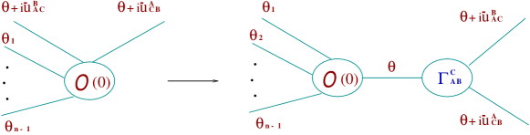
Figure 4.2: Bound state residue equation for form factors: ${F_{n+1}^{\mathcal{O}}\rightarrow F_{n}^{\mathcal{O}}}$.

A very important feature which distinguishes the former properties 1-4 from the ones we are going to recall now is the fact that the first ones are based on very general principles and therefore do not require any information about the particular nature of the operator $\mathcal{O}$ under consideration. However, it was already pointed out in the introduction of this chapter that, once the assumption that each different solution to the form factor consistency equations corresponds to a different local operator is made [22], there are different ways to identify and constrain the nature of such an operator. One of the most fruitful and useful ones is to look at the asymptotic behaviour of the corresponding form factors. The following two properties establish important constraints for this asymptotic behaviour.

Property 5: relativistic invariance

Since we are describing relativistically invariant theories we expect for an operator $\mathcal{O}$ with spin $s$

$$F_{n}^{\mathcal{O}|\mu_{1}\ldots\mu_{n}}(\theta_{1}+\lambda,\ldots,\theta_{n}+\lambda)=e^{s\lambda}F_{n}^{\mathcal{O}|\mu_{1}\ldots\mu_{n}}(\theta_{1},\ldots,\theta_{n})\,\,,$$ (4.7)

with $\lambda$ being an arbitrary real number. This equation establishes a first constraint on the asymptotic behaviour of the form factors.

Property 6: asymptotic bounds

To be able to associate a solution of the equations (4.2)-(4.6) to a particular operator, the following upper bound on the asymptotic behaviour which was derived in [161]

$$\left[F_{n}^{\mathcal{O}|\mu_{1}\ldots\mu_{n}}(\theta_{1},\ldots,\theta_{n})\right]_{i}\leq\,\Delta^{\mathcal{O}}$$ (4.8)

turns out to be very useful. Here $\Delta^{\mathcal{O}}$ denotes the conformal dimension of the operator $\mathcal{O}$ in the conformal limit. For convenience we introduced the short hand notation,

$$\lim_{\theta_{i}\rightarrow\infty}f(\theta_{1},\ldots,\theta_{n})=\textnormal{const.}e^{[f(\theta_{1},\ldots,\theta_{n})]_{i}\theta_{i}},$$ (4.9)

which later will turn out to be very useful.

The next important property of form factors we want to state is known as momentum space cluster property and has been analysed explicitly for several concrete 1+1-dimensional QFT’s [164, 152, 159, 165]. It also admits a perturbative interpretation by means of Weinberg’s power counting argument [22, 177, 15]. With respect to the former properties, the momentum space cluster property differs in two basic aspects: First, it is not known for the time being a proof which can be considered at the same footing as the proofs existing for the former properties 1-6. Second, whereas the properties 1-6 do not require any knowledge about the specific nature of the local operator $\mathcal{O}$, the cluster property captures at least part of the operator nature of the theory.

Property 7: momentum space cluster property

Cluster properties in space, i.e. the observation that far separated operators do not interact, are quite familiar in quantum field theories [175] for a long time. In 1+1 dimensions a similar property has also been noted in momentum space. For the purely bosonic case this behaviour can be explained perturbatively by means of Weinberg’s power counting theorem, see e.g. [22, 177]. As mentioned in section 4.1.1, the cluster property states for an $n$-particle form factor associated to an operator $\mathcal{O}$ that

$$\mathcal{T}_{1,\kappa}^{\lambda}F_{n}^{\mathcal{O}}(\theta_{1},\ldots,\theta_{n})\sim F_{\kappa}^{\mathcal{O}^{\prime}}(\theta_{1},\ldots,\theta_{\kappa})F_{n-\kappa}^{\mathcal{O}^{\prime\prime}}(\theta_{\kappa+1},\ldots,\theta_{n})\,\,,$$ (4.10)

where, for convenience we have introduced the operator

$$\mathcal{T}_{a,b}^{\lambda}:=\lim_{\lambda\rightarrow\infty}\prod_{p=a}^{b}T_{p}^{\lambda}\,$$ (4.11)

which will allow for concise notations. It is composed of the translation operator $T_{a}^{\lambda}$ which acts on a function of $n$ variables as

$$T_{a}^{\lambda}\,f(\theta_{1},\ldots,\theta_{a},\ldots,\theta_{n})\,\mapsto\,f(\theta_{1},\ldots,\theta_{a}+\lambda,\ldots,\theta_{n})\,\,\,,$$ (4.12)

therefore the operator $\mathcal{T}_{1,\kappa}^{\lambda}$ has the effect of shifting to infinity the first $\kappa$ rapities entering in $F_{n}^{\mathcal{O}}(\theta_{1},\ldots,\theta_{n})$.

Whilst Watson’s equations and the residue equations stated above, are operator independent features of form factors, the cluster property captures part of the operator nature of the theory. The cluster property (4.10) does not only constrain the solution, but eventually also serves as a construction principle in the sense that when given $F_{n}^{\mathcal{O}}$ we may employ (4.10) and construct form factors related to $\mathcal{O}^{\prime}$ and $\mathcal{O}^{\prime\prime}$.

Despite the fact that the cluster property has been analysed for several concrete models in [164, 152, 159, 165], and that the possibility of having form factors associated to different local fields of the massive QFT on the r.h.s. and l.h.s. of (4.10) was originally pointed out in [159], examples of such a situation were up to now absent in the literature. In other words, only self-clustering was encountered for all the specific local operators of the various QFT’s investigated in [164, 152, 159, 165]. This fact makes the outcome of the cluster-analysis carried out in this thesis for the $SU(3)_{2}$-HSG very remarkable, since it provides the first explicit example of a model where the form factors of different local operators can be obtained from each other via clustering. Therefore, our analysis gives definite support to the assertion that (4.10) constitutes a closed mathematical structure, which relates various different solutions and whose abstract nature still needs to be unraveled.

Property 8: locality

Finally, we would like to mention a very important property of form factors for which, similarly to the momentum space cluster property, it does not exist such a well established proof as for the mentioned consistency properties 1-6, but which is really the confirmation that the objects we want to construct characterise a well defined QFT. This property is the locality of the operators $\mathcal{O}$ arising in (4.1) which is expressed, in the bosonic case, by means of the usual condition (see for instance [15]):

$$[\mathcal{O}_{1}({x}),\mathcal{O}_{2}({y})]=0,$$ (4.13)

for ${x}$ and ${y}$ to be causally disconnected points in Minkowski’s space and $\mathcal{O}_{1},\mathcal{O}_{2}$ two local operators of the QFT. As mentioned above, properties 1-4 do not require any information about the particular nature of the operator $\mathcal{O}$. Therefore, once a solution to these consistency equations is found, it is of great interest to check that the locality of the operator involved is guaranteed namely, properties 1-4 and locality are self-consistent requirements. A proof of the locality property involves the computation of correlation functions of the form

$$\langle 0|[\mathcal{O}_{1}({x}),\mathcal{O}_{2}({y})]|0\rangle,$$ (4.14)

which is possible once the form factors associated to the operator $\mathcal{O}_{1},\mathcal{O}_{2}$ are known, as we explain in more detail in the next subsection. Therefore, proving that such a correlation function vanishes whenever the points ${x},{y}$ are not causally connected is equivalent to demonstrate the locality of any operator whose form factors have been obtained as solutions to the previous consistency equations. In this direction, the work carried out in [168] provided a proof of locality for bosonic QFT’s whose particle spectrum does not contain stable bound states, so that property 4 does not enter the form factor analysis. An analysis concerning the locality property within the form factor approach may be also found in appendix B of [153], although the arguments exhibited there still lack the rigour of the proofs of properties 1-6 and are concerned with the specific case of bosonic QFT’s which do not contain stable bound states. Furthermore, the analysis performed in [153] holds for a particular choice of one of the operators $\mathcal{O}_{1}$, $\mathcal{O}_{2}$ so that Eq. (4.14) is not proven for the generality of local operators of the QFT’s under consideration.

4.1.2 Summarising the key steps of the solution procedure

Before we enter the different applications of form factors, we want to anticipate very generically and briefly the main steps of a possible solution procedure leading to the construction of form factors:

Solving Watson’s equations

The starting point in the solution procedure consists of finding an ansatz for the solution to the two first properties of form factors, the so-called Watson’s equations. A formal ansatz for such a solution was already provided in the original papers [22],

$$F_{n}^{\mathcal{O}|\mu_{1}\cdots\mu_{n}}=Q_{n}^{\mathcal{O}|\mu_{1}\cdots\mu_{n}}(\theta_{1},\cdots,\theta_{n})\,K_{n}^{\mu_{1}\cdots\mu_{n}}(\theta_{1},\cdots,\theta_{n}).$$ (4.15)

where $Q_{n}^{\mathcal{O}|\mu_{1}\cdots\mu_{n}}(\theta_{1},\cdots,\theta_{n})$ is assumed to be a function of the rapidities which neither contains zeros nor poles in the physical sheet and $K_{n}^{\mu_{1}\cdots\mu_{n}}(\theta_{1},\cdots,\theta_{n})$ encodes the pole structure of the form factors revealed by Eqs. (4.4) and (4.6) and does not depend on the particular nature of the operator at hand. Additional properties of these two functions, more concretely, the symmetries of the former and the pole structure of the latter, can be imposed thereafter by appealing to the particular features of the model under consideration. In particular, it is common to assume the following structure for the $K$-function

$$K_{n}^{\mu_{1}\cdots\mu_{n}}(\theta_{1},\cdots,\theta_{n})=\prod_{i<j}\frac{F_{\text{min}}^{ij}(\theta_{ij})}{P_{ij}(\theta_{ij})},$$ (4.16)

where the functions $F_{\text{min}}^{ij}(\theta_{ij})$ are the so-called minimal form factors, whose properties will be introduced in subsection 4.3, and $P_{ij}(\theta_{ij})$ are functions which capture the pole structure of the form factors. In this fashion, the ansatz (4.15) can be chosen in such a way that Watson’s equations are automatically satisfied.

Solving the kinematical and bound state residue equations

The next step consists of “plugging” the previous ansatz into Eqs. (4.4) and (4.6). This gives rise to two recursive Eqs. relating the $(n+2)$- and $n$-particle form factors and the $(n+1)$- and $n$-particle form factors, respectively. The finding of general solutions to these equations is one of the hardest parts, and so far least systematic, of the whole analysis and, as mentioned before, in many cases one is only able to find solutions for the first lowest values of $n$ and/or for particular local operators. There is not an established procedure to solve in total generality such sort of recursive equations and furthermore, this solution becomes much more involved when both equations are present at the same time, namely when the model possesses stable bound states and property 4 enters the analysis. In order to get a first glimpse at the the general behaviour it is usually advantageous to analyse at first models which do not contain bound states, such that one only has to solve Eq. (4.4). We will also proceed this way for the HSG-models and find that, even in the situation when Eq. (4.6) does not arise, the finding of general close formulae for all $n$-particle form factors associated to any local operator of the QFT is highly non-trivial.

Identifying and constraining the nature of the operator

Having found a solution to the recursive Eqs.(4.4), and possibly (4.6) in case stable bound states are present, there is left the task to identify the concrete operator of the QFT to which these solutions correspond to. This is not known a priori, since properties 1-4 do not involve any anticipation of the nature of such an operator. Numerous authors [22, 153, 152, 155, 157, 158, 159, 160, 161, 27] have used various ways to identify and constrain the specific nature of the operator: by looking at asymptotic behaviours, performing perturbation theory, taking symmetries into account, formulating quantum equations of motion, etc. Our analysis will especially exploit the conjecture that each local operator of the massive QFT has a counterpart in the ultraviolet CFT whose primary operator content is, for the models at hand, well classified [59, 60, 61].

4.1.3 Correlation functions from form factors

Once the $n$-particle form factors corresponding to two particular operators $\mathcal{O},\mathcal{O}^{\prime}$ are known one is in principle in the position to compute the correlation function $\langle\mathcal{O}(r)\mathcal{O}^{\prime}(0)\rangle$. First of all, this correlation function can be rewritten in terms of form factors as follows,

$$\langle\mathcal{O}(r)\mathcal{O}^{\prime}(0)\rangle = \sum_{n=1}^{\infty}\sum_{\mu_{1},\cdots,\mu_{n}=1}^{N}\int{\frac{{d\theta_{1}}\cdots{d\theta_{n}}}{{n!}(2\pi)^{n}}\langle 0|\mathcal{O}(r)|V_{\mu_{1}}(\theta_{1})\cdots V_{\mu_{n}}(\theta_{n})\rangle}$$ (4.17)

$$\,\,\,\,\,\,\,\,\,\,\,\,\,\,\,\,\,\,\,\,\,\,\,\,\,\,\,\,\,\,\times\,\langle V_{\mu_{1}}(\theta_{1})\cdots V_{\mu_{n}}(\theta_{n})|\mathcal{O}(0)|0\rangle$$

where we have introduced the following orthogonal projector $P$,

$$P=\sum_{n=0}^{\infty}\sum_{\mu_{1},\cdots,\mu_{n}=1}^{N}\int{\frac{{d\theta_{1}}\cdots{d\theta_{n}}}{{n!}(2\pi)^{n}}|V_{\mu_{1}}(\theta_{1})\cdots V_{\mu_{n}}(\theta_{n})\rangle\langle V_{\mu_{1}}(\theta_{1})\cdots V_{\mu_{n}}(\theta_{n})|}$$ (4.18)

and the first sum runs over all the $n$-particle states while the second one runs over all the possible particle types in the theory, which we denote generically by $N$. It is easy to prove that $P$ is a projector namely, $P^{2}=I$ and $P^{\dagger}=P$, provided the states are normalised as

$$\langle V_{\mu_{1}}(\theta_{1})\cdots V_{\mu_{n}}(\theta_{n})|V_{\mu_{1}^{\prime}}(\theta_{1}^{\prime})\cdots V_{\mu_{n}^{\prime}}(\theta_{n}^{\prime})\rangle=\prod_{i=1}^{n}2\pi\delta_{\mu_{i}\mu_{i}^{\prime}}\delta(\theta_{i}-\theta_{i}^{\prime}),$$ (4.19)

which can be derived from Eq. (2.61).

In order to rewrite (4.17) in terms of form factors, we only need to be able to shift the first matrix element appearing in (4.17) to a matrix element located at the origin. For this purpose we must consider the action of a translation of the Poincaré group $U_{T_{{x}}}$ on the operator $\mathcal{O}({x})$ and the vertex operators $V_{\mu_{i}}(\theta_{i})$,

$$U_{T_{x}}\mathcal{O}(0)U_{T_{x}}^{-1}=\mathcal{O}({x}),\,\,\,\,\,\,\,\,\textnormal{and}\,\,\,\,\,\,\,\,U_{T_{x}}V_{\mu_{i}}(\theta_{i})U_{T_{x}}^{-1}=e^{ip^{\nu}(\theta_{i})x_{\nu}}V_{\mu_{i}}(\theta_{i}).$$ (4.20)

Therefore, we obtain

$$\langle 0|\mathcal{O}(r)|V_{\mu_{1}}(\theta_{1})\cdots V_{\mu_{n}}(\theta_{n})\rangle=\exp\left(-r\sum_{i=1}^{n}m_{\mu_{i}}\cosh\theta_{i}\right)\langle 0|\mathcal{O}(0)|V_{\mu_{1}}(\theta_{1})\cdots V_{\mu_{n}}(\theta_{n})\rangle$$ (4.21)

for $p_{0}(\theta_{i})=m_{\mu_{i}}\cosh(\theta_{i})$, for $m_{\mu_{i}}$ to be the mass of the particle $\mu_{i}$. Here we have taken $x^{\nu}=(-ir,0)$ in order to guarantee that $x^{2}=-r^{2}<0$ and, consequently, that the operators involved in the correlation function (4.22) are located at causally connected space positions.

Consequently, the correlation function (4.17) can finally be expressed in terms of $n$-particle form factors of the local operators $\mathcal{O}$ and $\mathcal{O}^{\prime}$ as

$$\left\langle\mathcal{O}(r)\mathcal{O}^{\prime}(0)\right\rangle = \sum_{n=1}^{\infty}\sum_{\mu_{1}\ldots\mu_{n}}\int\limits_{-\infty}^{\infty}\ldots\int\limits_{-\infty}^{\infty}\frac{d\theta_{1}\ldots d\theta_{n}}{n!(2\pi)^{n}}\exp\left(-r\sum_{i=1}^{n}m_{\mu_{i}}\cosh\theta_{i}\right)$$ (4.22)

$$\times\,\,F_{n}^{\mathcal{O}|\mu_{1}\ldots\mu_{n}}(\theta_{1},\ldots,\theta_{n})\,\left(F_{n}^{\mathcal{O}^{\prime}|\mu_{1}\ldots\mu_{n}}(\theta_{1},\ldots,\theta_{n})\,\right)^{*}.$$

The possibility to compute correlation functions from form factors may be exploited to explicitly evaluate various quantities, in particular those provided before by the TBA-analysis. In particular, the Virasoro central charge of the underlying CFT by means of the so-called Zamolodchikov’s $c$-theorem and the identification of the operator content of the QFT. This is explained in more detail in the next subsections.

4.1.4 Numerical methods

Before we enter the analysis of the specific quantities we may be able to compute once the form factors associated to a certain local operator are known, we want to comment very briefly on the numerical methods which will be employed later for the explicit evaluation of correlation functions through Eq. (4.22). In this thesis, we have concentrated on the emphasis of the physics rather than indulging too much into numerical technicalities. However, since this part of the work also required considerable effort, we want to give at least a flavour of what is involved.

Since many quantities we are interested in are at the moment not accessible in an analytic way, the numerical part is rather essential. Without this numerical part the outcome of our study will get considerably reduced since, ultimately, only by explicitly computing the Virasoro central charge, the conformal dimensions of various local operators of the theory, Zamolodchikov’s $c$-function etc… we will be in the position to claim that our form factor solutions are perfectly consistent with the physical picture anticipated for the models under consideration. Therefore, the expressions obtained will not be merely interesting from a mathematical point of view but also will enter the numerical evaluation of physical quantities.

As mentioned above, the main difficulty of the numerical analysis is the evaluation of the multi-dimensional integrals arising in the expansion (4.22) of the correlation functions. In general, the two-particle contribution can be evaluated even analytically once a suitable change of variables is performed (we will see explicit examples later). Therefore, at this stage, no sophisticated numerical tools are really needed. However, although the two-particle contribution is in most cases the leading one, we will see in the course of our specific analysis that the results obtained at this order are still very far from the expected ones, and that one has to sum at least up to 4-particle contribution to obtain reasonably accurate values. The computation of the 3- and 4-particle contributions can usually be performed by using the MATHEMATICA program. However, the evaluation of 5-, 6-, 7- or 8-particle contributions requires a lot of computer time and can not be carried out in the same way. Due to the latter reason, we have resorted to a FORTRAN code which makes use of the widely used numerical recipe routine VEGAS [179] for the evaluation of the multi-dimensional integrals. In this fashion we have been able to obtain different correlation functions in the 8-particle approximation in computing times always lower than one hour. We believe that more elaborated programs and/or the use of faster computers will allow for reducing considerably the computing time and eventually evaluate the correlation functions up to a much higher order. However, in many cases we have been content with the results obtained at this order and also we never intended to focus our analysis on the investigation and perfection of the numerical methods themselves, but to compute physical quantities with an accuracy and time cost which always justify the computational effort.

4.1.5 Virasoro central charge from form factors

One of the main purposes of our form factor analysis is to provide an additional check of the consistency of the S-matrices proposed in [51] to describe the HSG-models at quantum level. The results arising from the TBA-analysis carried out in chapter 3 gave rise to a physical picture which was in complete consistency with the mentioned S-matrix proposal and in particular allowed for the identification of the Virasoro central charge of the underlying CFT, a WZNW-coset theory associated in our case to cosets of the form $G_{k}/U(1)^{\ell}$, whose Virasoro central charge is given by Eq. (2.123). At the same time, as indicated in section 4.1.3, once the $n$-particle form factors are known one might be able to compute correlation functions by means of (4.22) and consequently obtain also the ultraviolet Virasoro central charge of the underlying CFT by means of (4.32), the so-called $c$-theorem of Zamolodchikov [24]. Leaving for section 4.10 the study of the RG-flow of Zamolodchikov’s $c$-function, we want to present now the key results which might lead us to extract the Virasoro central charge in the form factor framework and therefore double-check one of the most important data provided by the TBA, surpassing at the same time the results of the latter analysis.

Let us start by summarising the information contained in the $c$-theorem of Zamolodchikov [24]: For any 1+1-dimensional renormalisable and unitary QFT there exists a function $c(g_{1},\cdots,g_{i},\cdots)$ of the coupling constants ${g_{i}}$ of the theory, having the following properties:

i) it is non-increasing along renormalisation group trajectories, namely

$$\frac{dc({\mathbf{g}})}{dt}\leq 0,$$ (4.23)

for $t$ to be the renormalisation group parameter,

ii) it is stationary at critical fixed points, usually denoted by ${\mathbf{g}}={\mathbf{g}}^{*}$, at which the 1+1-dimensional QFT acquires an infinite conformal symmetry generated as usual by a Virasoro algebra (see subsection 2.1.1 in chapter 2). If we recall the definition of the $\beta_{i}({\mathbf{g}})$-functions as the “velocities” of change of the renormalised coupling constants along the renormalisation group flow [178],

$$\beta_{i}({\mathbf{g}})=-\frac{dg_{i}}{dt},$$ (4.24)

property ii) is equivalently expressed by saying that these $\beta_{i}$-functions are vanishing at critical fixed points,

$$\beta_{i}({\mathbf{g}}^{*})=0\,\,\,\,\,\Leftrightarrow\,\,\,\,\,{\left[\frac{\partial c({\mathbf{g}})}{\partial g_{i}}\right]}_{{\mathbf{g}}={\mathbf{g}}^{*}}=0,$$ (4.25)

therefore $c({\mathbf{g}}^{*})$ is stationary at renormalisation group critical fixed points,

iii) in fact, the $c$-theorem also establishes that the function $c({\mathbf{g}})$ reduces at these fixed points to the Virasoro central charge of the corresponding conformal field theory. It is the latter property which we will exploit in this and the next chapter in order to obtain the central charge corresponding to the $SU(N)_{2}/U(1)^{N-1}$-coset models. Having this aim in mind, the fundamental result we wish to employ was also established in [24] and can be summarised as follows [4, 163]: Let us consider the local operators $\Theta$, $T$ and $\bar{T}$ corresponding to the components of the energy momentum tensor of spin 2, 0 and -2 respectively and define the following functions

$$F(z\bar{z}) := z^{4}\langle T(z,\bar{z})T(0,0)\rangle,$$ (4.26)

$$G(z\bar{z}) := z^{3}\bar{z}\langle T(z,\bar{z})\Theta(0,0)\rangle,$$ (4.27)

$$H(z\bar{z}) := z^{2}\bar{z}^{2}\langle\Theta(z,\bar{z})\Theta(0,0)\rangle,$$ (4.28)

in terms of the usual complex coordinates $z=x^{0}+ix^{1},\bar{z}=x^{0}-ix^{1}$. The various components of the energy momentum tensor are interrelated by means of its conservation law

$$\partial_{\bar{z}}T+\frac{1}{4}\partial{\Theta}=0.$$ (4.29)

The correlation function of the previous equation with $T(0,0)$ and $\Theta(0,0)$, with the help of the definitions (4.26)-(4.28) gives rise to the following identity,

$$\frac{dc}{dt}=-\frac{3}{4}H,$$ (4.30)

for $t=\ln(m^{2}z\bar{z})=2\ln(mr)$, $m$ being a fixed mass scale, $r$ the radial distance and

$$c(t)=c(mr):=2F-G-\frac{3}{8}H.$$ (4.31)

Notice that, this function $c$ is always non-increasing, since the definition (4.28) ensures that $H\geq 0$. It is also stationary at critical fixed points where $\Theta=0$ and therefore $H$ vanishes too. In fact, at critical fixed points also the function $G$ vanishes for the same reason and (4.31) reduces to $F=c/2$, relation which in a conformal field theory defines $c$ as its Virasoro central charge [2, 3] (see also subsection 2.1.1 of chapter 2). Consequently, the function (4.31) fulfills properties i), ii) and iii) and can be identified as the same function these properties referred to at the beginning of this subsection.

By integrating now Eq. (4.30) we obtain for the difference between the ultraviolet and infrared Virasoro central charges,

$$c_{uv}-c_{ir}=\Delta c=\frac{3}{4}\int\limits_{-\infty}^{\infty}H(t)dt=\frac{3}{2}{\int_{0}^{\infty}}drr^{3}\langle\Theta(r)\Theta(0)\rangle,$$ (4.32)

where we used the definition of $H$ in terms of the trace of the energy momentum tensor (4.28) and $t=2\ln(mr)$. Recall that, due to the conservation of the energy momentum tensor, it has been possible to express the $c$-function, initially given in terms of several correlators involving all the components of the energy momentum tensor (4.31) in terms of only the correlation function of its trace. Taking into account that the infrared central charge is zero for purely massive theories, Eq. (4.32) gives the ultraviolet central charge of the corresponding underlying CFT. Very remarkably, whereas on the l.h.s. we have a quantity characterising the ultraviolet conformal field theory, on the r.h.s. we have the trace of the energy momentum tensor, a local operator of the perturbed conformal field theory or, in other words, a quantity defined away from the critical fixed point.

Being formula (4.32) available we only need now to use (4.22) to express the correlation function of $\Theta$ in terms of form factors of the same operator. By doing so, and performing thereafter the $r$-integration we get the following expression for the central charge,

$$\Delta c=9\sum_{n=1}^{\infty}\sum_{\mu_{1}\ldots\mu_{n}}\int\limits_{-\infty}^{\infty}\ldots\int\limits_{-\infty}^{\infty}\frac{d\theta_{1}\ldots d\theta_{n}}{n!(2\pi)^{n}\left(\sum_{i=1}^{n}m_{\mu_{i}}\cosh\theta_{i}\right)^{4}}\left|F_{n}^{\mathcal{O}|\mu_{1}\ldots\mu_{n}}(\theta_{1},\ldots,\theta_{n})\right|^{2}\,\,,$$ (4.33)

which can now in principle be computed provided all $n$-particle form factors of the energy momentum tensor are known.

4.1.6 Ultraviolet conformal dimensions from form factors

As indicated at the beginning of this chapter, there are two assumptions which turn out to be crucial in the form factor analysis: We will assume the existence of a one-to-one correspondence between the operator content of the underlying CFT and the massive QFT and between the solutions to the form factor consistency equations of subsection 4.1.1 and the local operators of the massive QFT. Provided these two assumptions are made, it is clear that the re-construction or identification of the operator content of the massive QFT can be performed by directly identifying for each local operator of the massive QFT its corresponding counterpart in the UV-limit. Since the operator content of the underlying CFT is well classified for all the HSG-models [59, 60, 61], one is left with the task of matching our form factor solutions with the operators of the underlying CFT. In our case, we will carry out such an identification by extracting the ultraviolet conformal dimensions of those local operators of the QFT for which we have previously computed all $n$-particle form factors (see section 4.4).

There are various ways to determine the ultraviolet conformal dimensions of the operators of the massive QFT. We may use the fact that the values of $\Delta^{\mathcal{O}}$ are obtainable when we exploit our knowledge about the underlying CFT more deeply. Considering an operator which in the conformal limit corresponds to a primary field we can of course compute the conformal dimension by appealing to the UV-limit of the two-point correlation function

$$\left\langle\mathcal{O}_{i}(r)\mathcal{O}_{j}(0)\right\rangle=\sum_{k}C_{ijk}\,r^{2\Delta_{k}-2\Delta_{i}-2\Delta_{j}}\,\left\langle\mathcal{O}_{k}(0)\right\rangle+\ldots$$ (4.34)

The three-point couplings $C_{ijk}$ are independent of $r$. In particular when assuming that $0$ is the smallest conformal dimension occurring in the model (which is the case for unitary models), we have (see section 2.1 in chapter 2),

$$\lim_{r\rightarrow 0}\left\langle\mathcal{O}(r)\mathcal{O}(0)\right\rangle\sim r^{-4\Delta^{\!\!\mathcal{O}}}\,\,\qquad\qquad\text{for }r\ll\left(\frac{C_{\Delta^{\mathcal{O}}\Delta^{\mathcal{O}}\,0}}{C_{\Delta^{\mathcal{O}}\Delta^{\mathcal{O}}\Delta^{\mathcal{O}^{\prime\prime}}}\left\langle\mathcal{O}^{{}^{\prime\prime}}\right\rangle}\right)^{1/2\Delta^{\mathcal{O}^{\prime\prime}}}\,.$$ (4.35)

Here $\mathcal{O}^{\prime\prime}$ is the operator with the second smallest dimension for which the vacuum expectation value is non-vanishing. Using a Lorentz transformation to shift the $\mathcal{O}(r)$ to the origin and expanding the correlation function in terms of form factors in the usual fashion, as presented in (4.22) we can compute the l.h.s. of (4.35) and extract $\Delta^{\!\!\mathcal{O}}$ thereafter. The disadvantage to proceed in this way is many-fold. First we need to compute the multidimensional integrals in (4.22) for each value of $r$, which means to produce a proper curve requires a lot of computational (at present computer) time. Second, for very small $r$ the $n$-th term within the sum is proportional to ($\log(r))^{n}$ such that we have to include more and more terms in that region whereas, at the same time, the expressions of the form factors and consequently, the integrals one has to evaluate, become more and more complicated (see appendix B) as $n$ increases. For that reason, the identification of the conformal dimension $\Delta^{\mathcal{O}}$ turns out to be very difficult, unless one has already a relatively good guess for its value, which is our case. Finally, the precise values of the lowest non-vanishing form factors, i.e. in general vacuum expectation values or one particle form factors are needed in order to compute the r.h.s. of (4.22). This is due to the fact that the constants $H^{\mathcal{O}|\tau,m}$ occurring in (4.75) are precisely fixed by the lowest non-vanishing form factor.

A short remark is also due concerning solutions related to different sets of $\mu$’s. The sum over the particle types in (4.22) simplifies considerably when taking into account that form factors corresponding to two sets, which differ only by a permutation, lead to the same contribution in the sum. This follows simply by using the first of Watson’s equations [22, 153, 152, 154, 155]. Recall that this property states that when two particles are interchanged we will pick up the related two particle scattering matrix as a factor (4.2). Noting that the scattering matrix is a phase, the expression remains unchanged.

Most of the disadvantages, which emerge when using (4.35) to compute the conformal dimensions, can be circumvented by formulating sum rules in which the $r$-dependence has been eliminated. Such type of rule has for instance been formulated by F. Smirnov [164] already more than a decade ago. However, the rule stated there is slightly cumbersome in its evaluation and we will therefore resort to one found more recently by G. Delfino, P. Simonetti and J.L. Cardy [27]. In close analogy to the spirit and derivation of the $c$-theorem [24], these authors derived an expression for the difference between the ultraviolet and infrared conformal dimension of a primary field $\mathcal{O}$

$$\Delta_{uv}^{\!\!\mathcal{O}}-\Delta_{ir}^{\!\!\mathcal{O}}=-\frac{1}{2\left\langle\mathcal{O}\right\rangle}\int\limits_{0}^{\infty}r\left\langle\Theta(r)\mathcal{O}(0)\right\rangle\,dr\,\,.$$ (4.36)

Using the expansion of the correlation function in terms of form factors ( 4.22) we may carry out the $\ r$-integration in (4.36) and obtain

$$\Delta_{uv}^{\!\!\mathcal{O}}-\Delta_{ir}^{\!\!\mathcal{O}} = -\frac{1}{2\left\langle\mathcal{O}\right\rangle}\sum_{n=1}^{\infty}\sum_{\mu_{1}\ldots\mu_{n}}\int\limits_{-\infty}^{\infty}\ldots\int\limits_{-\infty}^{\infty}\frac{d\theta_{1}\ldots d\theta_{n}}{n!(2\pi)^{n}\left(\sum_{i=1}^{n}m_{\mu_{i}}\cosh\theta_{i}\right)^{2}}$$ (4.37)

$$\times F_{n}^{\Theta|\mu_{1}\ldots\mu_{n}}(\theta_{1},\ldots,\theta_{n})\,\left(F_{n}^{\mathcal{O}|\mu_{1}\ldots\mu_{n}}(\theta_{1},\ldots,\theta_{n})\,\right)^{*}\,\,\,.$$

Notice also that, unlike in the evaluation of the $c$-theorem, which deals with a monotonically increasing series, due to the fact that it only involves absolute values of form factors, the series (4.36) can in principle be alternating. It is now worth to pause for a while and appreciate the advantages of this formula in comparison with (4.35). First of all, since the $r$-dependence has been integrated out we only have to evaluate the multidimensional integrals once. Second, the evaluation of (4.37) does not involve any anticipation of the value of $\Delta^{\!\!\mathcal{O}}$. Third, due to the fact that in the standard form factor construction form factors related to a local operator $\mathcal{O}$ are always normalised with respect to the lowest non-vanishing form factor, when the latter is the vacuum expectation value, the factor $\left\langle\mathcal{O}\right\rangle$ in (4.37) will cancel and its knowledge is not required at all in the analysis. Most important, fourth, the difficulty to identify the suitable region in $r$ which is governed by the $(\log r)^{n}$ behaviour of the $n$-th term in the sum in (4.22) and the upper bound in (4.34) have completely disappeared.

There are however little drawbacks for theories with internal symmetries and for the case when the lowest non-vanishing form factor of the operator we are interested in is not the vacuum expectation value. The first problem arises due to the fact that the sum rule is only applicable for primary fields $\mathcal{O}$ whose two-point correlation function with the energy momentum tensor is non-vanishing. We will see later that in fact this restricts quite severely the amount of operators for which we can actually use formula (4.36).

Notice that both (4.32) and (4.36) are equations which relate quantities characterising the ultraviolet CFT or critical, to a correlator which involves operators of the massive QFT namely, “off-critical” objects. Recall also that the identification of conformal dimensions in the TBA-context was only possible in principle for the perturbing operator (see section 3.4). Therefore, via the $\Delta$-sum rule [27] or the direct study of the UV-behaviour of the two point functions (4.35), the form factor analysis is expected to provide more information about the underlying ultraviolet CFT than the TBA-analysis. In other words, by carrying out the form factor program, we expect to confirm and surpass the TBA-outcome.

4.1.7 Renormalisation group analysis: the ${c(t_{0})}$- and ${\Delta(t_{0})}$-flows

Denoting by $r$ the radial distance and by $t=2\ln(mr)$ the renormalisation group parameter, the functions $c(mr)$ and $\Delta(mr)$ were defined in [24] and [27] respectively, obeying the differential equations

$$\frac{dc(m\,r)}{dr} = -\frac{3}{2}\,r^{3}\left\langle\Theta(r)\Theta(0)\right\rangle$$ (4.38)

$$\frac{d\Delta(m\,r)}{dr} = \frac{1}{2\left\langle{\cal O}(0)\right\rangle}r\,\left\langle\Theta(r){\cal O}(0)\right\rangle\,\,.$$ (4.39)

The r.h.s. of these equations involves the two-point correlation functions of the trace of the energy-momentum tensor $\Theta$ and an operator ${\mathcal{O}}$, which is a primary field in the sense of [2]. In general these equations are integrated from $r=0$ to $r=\infty$ and one consequently compares the difference between the ultraviolet and the infrared fixed points. Proceeding this way, we get Eqs. (4.32), (4.36) presented before, which we may use in order to compute the Virasoro central charge and ultraviolet conformal dimensions. In order to exhibit the quantitative onset of the mass scale of the unstable particles we integrate these equations now from some finite value $t_{0}$ to infinity.

Restricting our attention to purely massive theories, we use the fact that for these theories the infrared central charges are zero, such that we are left with the following identity

$$c(r_{0})=\frac{3}{2}\int\limits_{r_{0}}^{\infty}dr\,r^{3}\,\,\left\langle\hat{\Theta}(r)\hat{\Theta}(0)\right\rangle\,\,.$$ (4.40)

Since ultimately the functions $c(t)$ and $\Delta(t)$ depend upon the dimensionless combination $r_{0}:=m\,r$ and the parameter $r$ in Eq. (4.40) is now just an integration variable, it is suitable for our purposes to perform the variable transformation $r\rightarrow r/m$ which shall allow for eliminating any explicit dependence on the mass scale $m$. This is achieved if, simultaneously, the trace of the energy-momentum tensor, $\Theta$, is normalized as $\hat{\Theta}(r)=\Theta(r/m)/m^{2}$. After the previous redefinitions both $r$ and $\hat{\Theta}(r)$ are dimensionless objects in Eq. (4.40). Consequently, also the lower limit of the integral in (4.40), which we will denote by $r_{0}$, is a dimensionless renormalisation group parameter. Apart from the elimination of the explicit dependence in the mass scale, the latter transformations are very useful in order to establish a direct comparison between our results in this context and the ones obtained in the TBA-framework. Recall that the finite size scaling function of the TBA was defined in Eq. (3.28) and denoted by $c(R)$. In the TBA-framework $R$ is also a dimensionless variable, which is given by $R=m_{1}T^{-1}$, $T$ being the temperature of the system, namely, the energy scale, and $m_{1}$ being the mass of the lightest particle in the spectrum. In order to compare the results obtained in both approaches (the TBA- and form factor approach), in particular, we want to compare the finite size scaling function (3.28) of the TBA with Zamolodchikov’s $c$-function given by (4.40), one can draw now a formal analogy between the parameters $R$ and $r_{0}$. It is important to notice that the normalisation of the energy momentum tensor giving rise to the dimensionless operator $\hat{\Theta}$ does, of course, involve an equivalent modification of the corresponding form factors presented in appendix B. Such modification is simply expressed as

$$F_{n}^{\hat{\Theta}}=\frac{F_{n}^{{\Theta}}}{m^{2}}\,\,\,\,\,\,\,\,\,\,\text{for}\,\,\,\,\,\,\,\,\,\,\hat{\Theta}=\frac{\Theta}{m^{2}}.$$ (4.41)

As is trivially inferred from the expressions given in appendix B, as a consequence of such redefinition the mass-dependence of the form factors of the energy momentum tensor vanishes.

Although the latter equation can be trivially obtained from (4.38), it must be said that such a function had not been analysed before in the literature and constitutes the natural counterpart, in the renormalisation group context, of the finite size scaling function (3.28) computed in the TBA-approach. In fact our numerical results will show for several concrete models that these two functions carry the same physical information and have the same general features, sharing the characteristic “staircase” pattern already encountered for the scaling function of the TBA.

As presented in subsection 4.1.5, instead of the integral representation (4.40), the $c$-function is equivalently expressible in terms of a sum of correlators involving also other components of the energy momentum tensor [24, 4] which can be eliminated by means of the conservation law (4.29). Recall that the HSG-models, for which we ultimately want to analyse the behaviour of the function (4.40), contain unstable particles in their spectrum, characterised by the resonance parameters $\sigma_{ij}$. Taking this observation into account, we expect the flow of $c(r_{0})$ to surpass various steps: Starting with $r_{0}=0$ and assuming the masses of the stable particles of the theory to be all of the same order, say $m_{a},m_{b},\cdots,m_{n}\sim m$, the theory will leave its ultraviolet fixed point and at a certain definite value, say $r_{0}=r_{u}$, one of the unstables particles will become massive with respect to the energy scale determined by $mr_{0}$ such that $c(r_{0}>r_{u})$ can be associated to a different CFT. It appears natural to identify this value as the point at which $c(r_{0})$ is half the difference between the two coset values of $c$ (see the specific analysis carried out in section 4.10).

In order to obtain an explicit expression for the masses of the unstable particles, it is convenient to recall at this point that the resonance parameters $\sigma_{ij}=-\sigma_{ij}$ enter the Breit-Wigner formula [89] in the following way: In general an unstable particle of type $\tilde{c}$ is described by complexifying the physical mass of a stable particle by adding a decay width $\Gamma_{\tilde{c}}$, such that it corresponds to a pole in the S-matrix as a function of the Mandelstam variable $s$ at $s=M_{R}^{2}=(M_{\tilde{c}}{}-i\Gamma_{\tilde{c}}/2)^{2}$ in the non physical sheet (for a more detailed discussion see e.g. [14]). As mentioned in [14] whenever $M_{\tilde{c}}\gg\Gamma_{\tilde{c}}$, the quantity $M_{\tilde{c}}$ admits a clear-cut interpretation as the physical mass. However, since this assumption is only required for interpretational reasons we will not rely on it. Transforming as usual in this context from $s$ to the rapidity plane and describing the scattering of two stable particles of type $a\,$and $b$ with masses $m_{a}$ and $m_{b}$ by an S-matrix $S_{ab}(\theta)$ as a function of the rapidity $\theta$, the resonance pole is situated at $\theta_{R}=\sigma-i\bar{\sigma}$, $\sigma$ being the resonance parameter. Identifying the real and imaginary parts of the pole then yields

$$M_{\tilde{c}}^{2}{}-\frac{\Gamma_{\tilde{c}}^{2}{}}{4} = m_{a}^{2}{}+m_{b}^{2}{}+2m_{a}m_{b}\cosh\sigma\cos\bar{\sigma}$$ (4.42)

$$M_{\tilde{c}}\Gamma_{\tilde{c}} = 2m_{a}m_{b}\sinh|\sigma|\sin\bar{\sigma}\,\,.$$ (4.43)

Eliminating the decay width from (4.42) and (4.43), we can express the mass of the unstable particles $M_{\tilde{c}}$ in the model as a function of the masses of the stable particles $m_{a},m_{b}$ and the resonance parameter $\sigma$. In the regime

$$e^{|\sigma|}>>\frac{m_{a}^{2}+m_{b}^{2}}{m_{a}m_{b}},$$ (4.44)

we obtain

$$M_{\tilde{c}}^{2}\sim\frac{1}{2}m_{a}m_{b}(1+\cos\bar{\sigma})\,\,e^{|\sigma|}\,,$$ (4.45)

which corresponds to a decay width

$$\Gamma\sim\frac{2\sin\bar{\sigma}}{1+\cos{\bar{\sigma}}}.$$ (4.46)

Notice the occurrence in Eq. (4.45) of the variable $me^{|\sigma|/2}$ for $m_{a}\sim m_{b}\sim m$ familiar from our TBA-analysis, which was introduced originally in [126] in order to describe massless particles, i.e. one may perform safely the limit $m\rightarrow 0,\sigma\rightarrow\infty$. Therefore one might be tempted to describe flows related to (4.45) as massless flows, interpretation which will be also supported by our numerical results in section 4.10.

It is also interesting to notice that the need for fulfilling the energetical requirement $M_{c}>m_{a}+m_{b}$ leads to the following threshold for the allowed values of the resonance parameter $\sigma$:

$$e^{|\sigma|}>2\,\frac{(m_{a}+m_{b})^{2}}{m_{a}m_{b}\,(1+\cos\bar{\sigma})},$$ (4.47)

in particular, for $m_{a}=m_{b}$, and $\bar{\sigma}=\pi/2$ which is the case for all the $SU(N)_{2}$-HSG models, we obtain the constraint $\sigma>\ln 8$. Such requirement is in agreement with the fact that very different results are obtained, both in the TBA- and form factor context, for small and large values of $\sigma$. In particular, the development of plateaux in the scaling functions is a feature which only occurs for values of the resonance parameter large enough (see section 4.10). However, from the scattering matrix point of view, the HSG S-matrices make perfect sense for any value of $\sigma$ and it is an open problem to investigate whether or not evidence for the threshold (4.47) can be found in the context of the scattering theory. Recently, this problem has been investigated in the context of the construction of S-matrices containing infinitely many resonance poles [112].

As a consequence of (4.45) we may relate the value of $r_{u}$ for different choices of the resonance parameter. This provides also a confirmation of the fact that the renormalisation group flow is indeed achieved by $m\rightarrow r_{0}\,m$. Increasing $r_{0}$ further, the energy scale of the stable particles will eventually be reached at, say at $r_{0}=r_{a},r_{b},\ldots,r_{n}$. Depending on the relative mass scales between the stable particles these points may coincide. Finally the flow will reach its infrared fixed point $c(r_{0}=r_{ir})=0$.

Likewise we can integrate Eq. (4.39)

$$\Delta(r_{0})=-\frac{1}{2\left\langle{\cal O}(0)\right\rangle}\int\limits_{r_{0}}^{\infty}dr\,r\,\,\left\langle\hat{\Theta}(r){\cal O}(0)\right\rangle\,\,,$$ (4.48)

which allows to keep track of the manner the operator contents of the various conformal field theories are mapped into each other. We used that all conformal dimensions vanish in the infrared limit. Here the same comments after Eq. (4.40) apply, so that $r_{0}$ is a dimensionless RG-parameter. Fortunately, we have that $\left\langle\hat{\Theta}(r){\cal O}(0)\right\rangle$ is proportional to $\left\langle{\cal O}(0)\right\rangle$ in many applications such that the vacuum expectation value $\left\langle{\cal O}(0)\right\rangle$ cancels often when evaluating (4.48). One should note, however, that (4.48) is only applicable to those operators for which its two-point correlator with the trace of the energy momentum tensor is non-vanishing, such that one may not be in the position to investigate the flow of the entire operator content by means of (4.48), as happened for the $SU(3)_{2}$-HSG model.

In order to evaluate (4.40) and (4.48) for a concrete model we have to compute the two-point correlation functions in some way. Obviously, in our case we will make use of the results of the form factor analysis to be presented in subsequent sections for the $SU(3)_{2}$-HSG model and in the next chapter for all the $SU(N)_{2}$-HSG models.

As we know, the two-point correlation functions occurring in (4.40) and (4.48), can be expanded in terms of form factors of the corresponding operators (4.22). Using this expansion we replace the correlation functions in (4.40) and (4.48) and perform the $r$-integrations thereafter. Thus we obtain

$$c(r_{0})=3\sum_{n=1}^{\infty}\sum_{\mu_{1}\ldots\mu_{n}}\int\limits_{-\infty}^{\infty}\frac{d\theta_{1}\ldots d\theta_{n}}{n!(2\pi)^{n}}\frac{(6+6r_{0}E+3r_{0}^{2}E^{2}+r_{0}^{3}E^{3})}{2E^{4}}e^{-r_{0}\,E}$$

$$\,\,\,\,\,\,\,\,\,\,\,\,\,\,\,\,\,\,\,\,\,\,\,\,\,\,\,\,\,\,\,\,\,\,\,\,\,\,\,\,\,\,\,\,\,\,\,\,\times\left|F_{n}^{\hat{\Theta}|\mu_{1}\ldots\mu_{n}}(\theta_{1},\ldots,\theta_{n})\right|^{2}$$ (4.49)

and

$$\Delta(r_{0})=-\frac{1}{2\left\langle{\cal O}(0)\right\rangle}\sum_{n=1}^{\infty}\sum_{\mu_{1}\ldots\mu_{n}}\int\limits_{-\infty}^{\infty}\frac{d\theta_{1}\ldots d\theta_{n}}{n!(2\pi)^{n}}\frac{(1+r_{0}E)e^{-r_{0}\,E}}{2E^{2}}$$

$$\,\,\,\times F_{n}^{\hat{\Theta}|\mu_{1}\ldots\mu_{n}}(\theta_{1},\ldots,\theta_{n})\left(F_{n}^{{\cal O}|\mu_{1}\ldots\mu_{n}}(\theta_{1},\ldots,\theta_{n})\,\right)^{\ast}\,.$$ (4.50)

with $E=\sum_{i=1}^{n}\hat{m}_{\mu_{i}}\cosh{\theta_{i}}$, where the masses $\hat{m}_{\mu_{i}}=m_{\mu_{i}}/m$ have been also normalised in terms of the overall mass scale $m$ in order to make the quantity $E$ dimensionless, achieving consistency with the dimensionless character of $r_{0}$.

4.1.8 Renormalisation group flow of ${\beta}$-like functions

As reported in section 4.1.5 (see Eq. (4.24), in case there is only one coupling constant $g$ in the model, the $\beta$-function should obey the defining equation

$$\beta(g)=\frac{dg}{d{t_{0}}},$$ (4.51)

for $t_{0}=2\ln r_{0}$ to be the RG-flow parameter, so that we can rewrite the latter equation as

$$\frac{r_{0}}{2}\frac{d}{d{r_{0}}}=\beta(g)\frac{d}{dg}.$$ (4.52)

Here we applied Eq. (4.51) to the coupling constant $g$ in order to extract the $\beta$-function on the r.h.s. of (4.52).

It is now our interest to construct a function which allows a more clear identification of the critical fixed points surpassed by the $c$-function along its RG-flow. It is clear that this purpose might be achieved as soon as we construct any function which is proportional to ${dc(t_{0})}/{d{t_{0}}}$. Therefore, following an idea originally used by Zamolodchikov in [108], let us define a “coupling constant” $g:=c_{\text{uv}}-c(t_{0})$ normalized in such a way that it vanishes at the ultraviolet fixed point. If we now apply Eq. (4.52) to this coupling constant we obtain the equation

$$\frac{r_{0}}{2}\frac{dc(r_{0})}{d{r_{0}}}=\beta(g).$$ (4.53)

Clearly from the above definition, whenever we find $\beta(\tilde{g})=0$, we can identify $\tilde{c}=c_{\text{uv}}-\tilde{g}$ as the Virasoro central charge of the corresponding CFT. In fact this is true irrespectively of the presence of the factor $1/2$ on the l.h.s., thus we will drop it out in what follows.

Hence, taking the data obtained from (4.49), we compute $\beta$ as a function of $g$ by means of (4.53). Analogously, we can define also a $\beta$-like function associated to the $\Delta(t_{0})$-function (4.50) presented above. The numerical computation of these $\beta$-functions will be presented in the next chapter for the $SU(N=4)_{2}$- and $SU(N=5)_{2}$-HSG models.

4.2 The ${SU(3)_{2}}$-HSG model

As stated already in subsection 3.4.1, when performing the TBA-analysis, the $SU(3)_{2}$-HSG model contains only two self-conjugate solitons (1,1) and (1,2). Aiming towards a more compact notation these two solitons are more conveniently denoted by “+” and “-”. Therefore, the corresponding non-trivial S-matrix elements [51] as functions of the rapidity $\theta$ read now

$$S_{\pm\pm}=-1\quad\quad\text{and}\quad\quad S_{\pm\mp}(\theta)=\pm\tanh\frac{1}{2}\left(\theta\pm\sigma-i\frac{\pi}{2}\right)\,\,.\;$$ (4.54)

Here $\sigma$ is the resonance parameter, whose physical meaning was already discussed both in chapters 2 and 3. Eq. (4.54) means the scattering of particles of the same type is simply described by the S-matrix of the thermal perturbation of the Ising model. Also the remaining amplitudes do not possess poles inside the physical sheet, such that the formation of stable particles via fusing is not possible. The latter characteristic means that the task of finding solutions to the form factor consistency equations (4.2)-(4.6) turns out to be a bit simpler, since the so-called bound-state residue equation (4.6) does not arise.

For vanishing resonance parameter $\sigma=0$ the amplitudes $S_{\pm\mp}$ coincide formally with the ones which describe the massless flow between the tricritical Ising and the critical Ising model as analysed in [173]. However, there is an important conceptual difference since we view the expressions (4.54) as describing the scattering of massive particles. This has important consequences on the construction of the form factors and in fact the solutions we will present later are different from the ones proposed in [173]. Furthermore we will construct all $n$-particle form factors associated to a large class of operators whereas in [173] only solutions for some particular numbers of particles and a restricted amount of operators where found . Recall that in the HSG setting the massless flow was recovered in the context of the TBA (see section 3.4.1), only as a subsystem in terms of specially introduced variables ${r^{\prime}}=\frac{r}{2}e^{\sigma/2}$ combining the inverse temperature $r$ and the resonance parameter $\sigma$. The occurrence of the combination of variables $re^{\sigma/2}$ (although for a different $r$-parameter) will be also encountered later in the context of the renormalisation group analysis.

The system (4.54) is of special interest since it constitutes probably the simplest example of a massive QFT involving two particles of distinct type. Nonetheless, despite the simplicity of the scattering matrix we expect to find a relatively involved operator content, since for finite resonance parameter the $SU(3)_{2}$-HSG model describes a WZNW-coset model with central charge $c=6/5$ perturbed by an operator with conformal dimension $\Delta=3/5$. It is expected from the classical analysis and has also been confirmed by the TBA-analysis that, whenever the resonance parameter $\sigma$ is finite, we find the same ultraviolet central charge and therefore the same operator content. For this reason, when computing quantities (usually numerically) in the UV-limit, it is really only interesting to distinguish the situations $\sigma\rightarrow\infty$ and $\sigma$ finite (in particular, we will set $\sigma=0$). One can trivially notice from (4.54) that

$$\lim_{\sigma\rightarrow\infty}S_{\pm\mp}=1,$$ (4.55)

which means that the theory decouples into two copies of the Ising model and therefore the corresponding Virasoro central charge is expected to be $\frac{1}{2}+\frac{1}{2}=1$ in this limit. The latter behaviour will also be consistently recovered in the context of form factors, in particular when computing the corresponding Virasoro central charge by means of (4.32) and when studying the asymptotics of form factors in the limit $\sigma\rightarrow\infty$.

The corresponding underlying CFT, a WZNW-$SU(3)_{2}/U(1)^{2}$-coset or $SU(3)_{2}$-para- fermion theory [59], has recently [170, 171] found an interesting application in the context of the construction of quantum Hall states which carry a spin and fractional charges.

4.3 Recursive equations and minimal form factors

Attempting now to solve the form factor consistency equations presented in subsection 4.1.1, and proceeding as usual in this context [22, 172], we start by making a factorisation ansatz which already extracts explicitly some of the singularity structure we expect to find. For the case at hand, property 3 tells us that we must have a kinematical pole at $i\pi$ when two particles are conjugate to each other. Therefore the following parameterisation

$$F_{n}^{\mathcal{O}|\stackrel{{\scriptstyle l\,\times\,\pm}}{{\overbrace{\mu_{1}\ldots\mu_{l}}}}\stackrel{{\scriptstyle m\,\times\,\mp}}{{\overbrace{\mu_{l+1}\ldots\mu_{n}}}}}(\theta_{1}\ldots\theta_{n})=H_{n}^{\mathcal{O}|\mu_{1}\ldots\mu_{n}}Q_{n}^{\mathcal{O}|\mu_{1}\ldots\mu_{n}}(x_{1}\ldots x_{n})\,\!\!\prod_{i<j}\!\!\frac{F_{\text{min}}^{\mu_{i}\mu_{j}}(\theta_{ij})}{\left(x_{i}^{\mu_{i}}+x_{j}^{\mu_{j}}\right)^{\delta_{\mu_{i}\mu_{j}}}},$$ (4.56)

where we introduced the variable $x_{i}=e^{\theta_{i}}$, is very convenient, since the mentioned poles have already been isolated in the denominator of (4.56). The $H_{n}^{\mathcal{O}|\mu_{1}\ldots\mu_{n}}$ are normalisation constants and the functions $F_{\text{min}}^{\mu_{i}\mu_{j}}(\theta_{ij})$ are the the so-called minimal form factors. They satisfy the following equations

$$F_{\text{min}}^{ij}(\theta)=F_{\text{min}}^{ji}(-\theta)S_{ij}(\theta)=F_{\text{min}}^{ji}(2\pi i-\theta)\,\,,$$ (4.57)

and have neither zeros nor poles in the physical sheet $0<\text{Im}(\theta)<\pi$. Then, if we further assume that the $Q_{n}^{\mathcal{O}|\mu_{1}\ldots\mu_{n}}(\theta_{1},\ldots,\theta_{n})$ are functions separately symmetric in the first $l$ and the last $m$ rapidities and in addition 2$\pi i$-periodic in all rapidities, the ansatz (4.56) solves Watson’s equations (4.2) and (4.3) by construction. At the same time, being symmetric in the first $l$ and the last $m$ rapidities the $Q_{n}^{\mathcal{O}|\mu_{1}\ldots\mu_{n}}(\theta_{1},\ldots,\theta_{n})$ have to be combinations of elementary symmetric polynomials in the first $l$ and last $m$ rapidities (see appendix A). In particular, we have

$$Q_{n}^{\mathcal{O}|\stackrel{{\scriptstyle l\,\times\,+}}{{\overbrace{\mu_{1}\ldots\mu_{l}}}}\stackrel{{\scriptstyle m\,\times\,-}}{{\overbrace{\mu_{l+1}\ldots\mu_{n}}}}}(x_{1},\ldots,x_{n})=Q_{n}^{\mathcal{O}|\stackrel{{\scriptstyle m\,\times\,-}}{{\overbrace{\mu_{l+1}\ldots\mu_{n}}}}\stackrel{{\scriptstyle l\,\times\,+}}{{\overbrace{\mu_{1}\ldots\mu_{l}}}}}(x_{l+1},\ldots x_{n},x_{1},\ldots x_{l})\,\,,$$ (4.58)

such that, provided a solution has been constructed for a particular ordering of the $\mu$’s, for example the upper sign in (4.56), we can obtain the solution for a permuted ordering by using the monodromy properties. Especially, the reversed order is obtained by applying Eq. (4.58). Despite the fact that we do not gain anything new, it is still instructive to verify (4.4) as a consistency check also for the different ordering. The monodromy properties allow some simplification in the notation and from now on we restrict our attention without loss of generality to the upper sign in (4.56). In addition, we deduce from Eq. (4.7) that for a spinless operator $\mathcal{O}$ the total degree of $Q_{n}^{\mathcal{O}}$ has to be

$$\left[Q_{n}^{\mathcal{O}}\right]=\frac{l(l-1)}{2}-\frac{m(m-1)}{2},$$ (4.59)

where the brackets $[\,\,\,]$ have the meaning explained in (4.9).

A solution for the minimal form factors i.e., of equations (4.57), is found to be

$$F_{\text{min}}^{\pm\pm}(\theta) = -i\sinh\frac{\theta}{2}$$ (4.60)

$$F_{\text{min}}^{\pm\mp}(\theta) = \mathcal{N}^{\pm}(\theta)\prod_{k=1}^{\infty}\tfrac{\Gamma(k+\frac{1}{4})^{2}\Gamma\left(k+\frac{1}{4}+\frac{i}{2\pi}(\theta\pm\sigma)\right)\Gamma\left(k-\frac{3}{4}-\frac{i}{2\pi}(\theta\pm\sigma)\right)}{\Gamma(k-\frac{1}{4})^{2}\Gamma\left(k-\frac{1}{4}-\frac{i}{2\pi}(\theta\pm\sigma)\right)\Gamma\left(k+\frac{3}{4}+\frac{i}{2\pi}(\theta\pm\sigma)\right)}\,\,$$ (4.61)

$$= \mathcal{N}^{\pm}(\theta)\exp\left(-\int\limits_{0}^{\infty}\tfrac{dt}{t}\tfrac{\sin^{2}\left((i\pi-\theta\mp\sigma)\frac{t}{2\pi}\right)}{\sinh t\cosh t/2}\right)\,=e^{\pm\tfrac{\theta}{4}}\tilde{F}_{\text{min}}^{\pm\mp}(\theta)\,\,.$$ (4.62)

Here $F_{\text{min}}^{\pm\pm}(\theta)$ is the well-known minimal form factor of the thermally perturbed Ising model [172, 154] and for the upper choice of the signs, Eq. (4.62) coincides for vanishing $\sigma$ up to normalisation with the expression found in [173]. We introduced the normalisation function

$$\mathcal{N}^{\pm}(\theta)=2^{\frac{1}{4}}\exp\left(\tfrac{i\pi(1\mp 1)\pm\theta}{4}-\tfrac{G}{\pi}\right)$$ (4.63)

with $G=0.91597$ being the Catalan constant.

The expression (4.62) can be derived by using a result dating back to the original literature [22, 172] which states that, once an integral representation for the S-matrix is known in the form

$$S_{\mu_{i}\mu_{j}}(\theta)=\exp{\Bigg{(}\int_{0}^{\infty}\frac{dt}{t}f_{\mu_{i}\mu_{j}}(t)\sinh{\Big{(}\frac{t\theta}{i\pi}\Big{)}}\Bigg{)}},$$ (4.64)

where $f_{\mu_{i}\mu_{j}}(t)$ is a certain function which depends on the particular theory under consideration, the corresponding minimal form factors are given, up to some normalisation constant $\mathcal{C}_{ij}$, by

$$F_{\text{mim}}^{\mu_{i}\mu_{j}}(\theta)=\mathcal{C}_{ij}\,\exp{\Bigg{(}\int_{0}^{\infty}\frac{dt}{t}f_{\mu_{i}\mu_{j}}(t)\frac{\sin{\Big{(}\frac{t(i\pi-\theta)}{2\pi}\Big{)}}^{2}}{\sinh(t)}\Bigg{)}}.$$ (4.65)

For all the HSG models, such an integral representation (4.64) was provided in chapter 3, and in order to get (4.62), we only need to particularise it to the $SU(3)_{2}$-HSG model at hand.

The minimal form factors (4.60), (4.62) possess various properties which we would like to employ in the course of our argumentation. They obey the functional identities

$$F_{\text{min}}^{\pm\pm}(\theta+i\pi)F_{\text{min}}^{\pm\pm}(\theta) = -\frac{i}{2}\sinh\theta,$$ (4.66)

$$F_{\text{min}}^{\pm\mp}(\theta+i\pi)F_{\text{min}}^{\pm\mp}(\theta) = \frac{i^{\frac{2\mp 1}{2}}\,e^{\pm\frac{\theta}{2}}}{\cosh\frac{1}{2}\left(\theta\pm\sigma-\frac{i\,\pi}{2}\right)}\,\,,$$ (4.67)

which are easily derived by using the representation (4.61) in terms of $\Gamma$-functions of the minimal form factors. We will also exploit the asymptotic behaviours

$$\lim\limits_{\sigma\rightarrow\infty}F_{\text{min}}^{\pm\mp}(\pm\theta)\sim e^{-\frac{\sigma}{4}},\qquad\left[F_{\text{min}}^{\pm\pm}(\theta_{ij})\right]_{i}=\frac{1}{2},\qquad\left[F_{\text{min}}^{\pm\mp}(\theta_{ij})\right]_{i}=\QATOPD\{.{0}{-1/2}\,\,,$$ (4.68)

which, together with the factorisation ansatz (4.56) and (4.59) lead us immediately to the relations

$$\left[F_{n}^{\mathcal{O}|l,m}\right]_{i} = \left[Q_{n}^{\mathcal{O}|l,m}\right]_{i}+\frac{1-l}{2}\qquad\qquad\,\,\,\text{for\quad}1\leq i\leq l$$ (4.69)

$$\left[F_{n}^{\mathcal{O}|l,m}\right]_{i} = \left[Q_{n}^{\mathcal{O}|l,m}\right]_{i}+\frac{m-l-1}{2}\,\,\quad\quad\text{for \quad}l<i\leq n\,,$$ (4.70)

where we recalled again (4.9). These relations are very useful in the identification process of a particular solution with a specific operator. Since we may restrict our attention to one particular ordering only, we abbreviate the r.h.s. of (4.56) from now on as $F_{n}^{\mathcal{O}|l,m}$ and similar for the $Q$’s.

By substituting now the ansatz (4.56) into the kinematic residue Eq. (4.4) the whole problem of determining the form factors associated to a particular local operator $\mathcal{O}$ reduces, with the help of (4.66) and (4.67), to solving the following recursive equations

$$Q^{\mathcal{O}|l+2,m}(-x,x,\ldots,x_{n})=D_{\vartheta}^{l,m}(x,x_{1},\ldots,x_{n})Q^{\mathcal{O}|l,m}(x_{1},\ldots,x_{n})$$ (4.71)

$$D_{\vartheta}^{l,m}(x,x_{1},\ldots,x_{n})=\frac{1}{2}(-ix)^{l+1}\sigma_{l}^{+}\sum_{k=0}^{m}(-ie^{\sigma}x)^{-k}(1-(-1)^{l+k+\vartheta}){\sigma}_{k}^{-}\,\,.$$ (4.72)

where $\sigma_{l}^{+}$ and ${\sigma}_{k}^{-}$ denote elementary symmetric polynomials of degrees $l$ and $k$ in the variables $x_{i}$ with $i=1,\cdots,l$ and $i=l+1,\cdots,l+m$ respectively. More information about the properties and definition of these polynomials may be found in appendix A and in [174]. In particular the use of the generating equation (A.4) is fundamental in order to obtain (4.72).

If we now set $l=2s+\tau$ and $m=2t+\tau^{\prime}$ then Eq. (4.72) can be rewritten as

$$D_{\zeta}^{2s+\tau,2t+\tau^{\prime}}(x,x_{1},\ldots,x_{n})=(-i)^{2s+\tau+1}\sigma_{2s+\tau}^{+}\sum_{p=0}^{t}x^{2s-2p+\tau+1-\zeta}\hat{\sigma}_{2p+\zeta}^{-}\,\,.$$ (4.73)

In (4.72) $\vartheta$ is related to the factor of local commutativity $\omega=(-1)^{\vartheta}=\pm 1$ introduced in (4.4). We introduced also the function $\zeta$ which is $0$ or $1$ for the sum $\vartheta+\tau$ being odd or even, respectively. We shall use various notations for elementary symmetric polynomials. We employ the symbol $\sigma_{k}$ when the polynomials depend on the variables $x_{i}$, the symbol $\bar{\sigma}_{k}$ when they depend on the inverse variables $x_{i}^{-1}$, the symbol $\hat{\sigma}_{k}$ when they depend on the variables $\hat{x}_{i}=x_{i}e^{-\sigma+i\pi/2}$ and $\tilde{\sigma}_{k}$ when we set the first two variables to $x_{1}=-x,$ $x_{2}=x$. The number of variables the polynomials depend upon is defined always in an unambiguous way through the l.h.s. of our equations, where we assume the first $l$ variables to be associated with $\mu=+$ and the last $m$ variables with $\mu=-$. In case no superscript is attached to the symbol the polynomials depend on all $m+l$ variables, and as indicated in the previous paragraph , in case of a “$+$” they depend on the first $l$ variables and in case of a “$-$” on the last $m$ variables.

The recursive equations for the constants turn out to be

$$H_{n+2}^{\mathcal{O}|l+2,m}=i^{m}2^{2l-m+1}e^{\sigma m/2}H_{n}^{\mathcal{O}|l,m}\,\,.$$ (4.74)

Fixing one of the lowest constants, the solutions to these equations read

$$H^{\mathcal{O}|2s+\tau,m}=i^{sm}2^{s(2s-m-1+2\tau)}e^{sm\sigma/2}H^{\mathcal{O}|\tau,m},\qquad\tau=0,1\,.$$ (4.75)

Note that at this point an unknown constant, that is $H^{\mathcal{O}|\tau,m}$, enters into the procedure. This quantity is not constrained by the form factor consistency equations and has to be obtained from elsewhere. Notice that there is a certain ambiguity contained in the equations (4.74), i.e. we can multiply $H_{n}^{\mathcal{O}|l,m}$ by $i^{2l}$, $i^{2l^{2}}$ or $(-1)^{l}$ and produce a new solution. However, since in practical applications we are usually dealing with the absolute values of the form factors, these ambiguities will turn out to be irrelevant.

4.4 The solution procedure

Solving recursive equations of the type (4.71) in complete generality is still an entirely open problem. Ideally, one would like to reach a situation similar to the one in the bootstrap construction procedure of the scattering matrices, where one can state general building blocks, e.g. particular combinations of hyperbolic functions whenever backscattering is absent [88], infinite products of gamma functions when backscattering occurs or elliptic functions when infinite resonances are present. Unfortunately, such a general analytical structure has not been encountered by now in the context of the form factor analysis. In fact, for most models, only a few solutions of (4.71) corresponding to the first smaller values of $n$ and/or to particular local operators have been constructed. Consequently, the results we present now for the $SU(3)_{2}$-HSG model and generalise thereafter for all the $SU(N)_{2}$-HSG models are very remarkable as the goal of constructing systematically all $n$-particle form factors associated to a large class of operators of the model has been achieved. Therefore, the form factor study we have performed for the $SU(3)_{2}$- and $SU(N)_{2}$-HSG models is not only relevant as a consistency check through (4.32) and (4.36) of the S-matrix proposal [51] and the results of the TBA-analysis, but also serves as an important contribution to the general understanding of the problem of finding general solutions to recursive problems of the type (4.71).

It will turn out that all solutions to the recursive equations (4.71) may be constructed from some general building blocks consisting out of determinants of matrices whose entries are elementary symmetric polynomials in some particular set of variables. Let us therefore define the ($t+s$)$\times$($t+s$)-matrix

$$\mathcal{\,}\left(\mathcal{A}_{l,m}^{\mu,\nu}(s,t)\right)_{ij}:=\QATOPD\{.{\sigma_{2(j-i)+\mu}^{+}\qquad\,\,\,\,\,\,\,\,\text{for\quad}1\leq i\leq t}{\hat{\sigma}_{2(j-i)+2t+\nu}^{-}\,\,\,\quad\quad\,\,\,\,\,\,\,\text{for\quad}t<i\leq s+t}\,\,.$$ (4.76)

The superscripts $\mu,\nu$ may take the values $0$ and $1$ and the subscripts $l,m$ characterise the number of different variables related to the particle species “$+$”, “$-$”, respectively. More explicitly the matrix $\mathcal{A}$ reads

$$\mathcal{A}_{l,m}^{\mu,\nu}=\left(\begin{array}[]{rrrrrr}\sigma_{\mu}^{+}&\sigma_{\mu+2}^{+}&\sigma_{\mu+4}^{+}&\sigma_{\mu+6}^{+}&\cdots&0\\ 0&\sigma_{\mu}^{+}&\sigma_{\mu+2}^{+}&\sigma_{\mu+4}^{+}&\cdots&0\\ \vdots&\vdots&\vdots&\vdots&\ddots&\vdots\\ 0&0&0&0&\cdots&\sigma_{2s+\mu}^{+}\\ \hat{\sigma}_{\nu}^{-}&\hat{\sigma}_{\nu+2}^{-}&\hat{\sigma}_{\nu+4}^{-}&\hat{\sigma}_{\nu+6}^{-}&\cdots&0\\ 0&\hat{\sigma}_{\nu}^{-}&\hat{\sigma}_{\nu+2}^{-}&\hat{\sigma}_{\nu+4}^{-}&\cdots&0\\ \vdots&\vdots&\vdots&\vdots&\ddots&\vdots\\ 0&0&0&0&\cdots&\hat{\sigma}_{2t+\nu}^{-}\end{array}\right)\,\,.$$ (4.77)

The different combinations of the integers $\mu,\nu,l,m$ will correspond to different kinds of local operators $\mathcal{O}$. These sort of determinant formulae, albeit with entirely different entries of symmetric polynomials, have occurred before in various places in the literature [158, 159, 152]. These type of expressions allow on one hand for systematic proofs, as we will demonstrate later, and on the other hand, they are claimed to be useful in the construction of correlation functions as suggested in [176]. In addition, the form factors will involve a function depending on two further indices $\bar{\mu}$ and $\bar{\nu}$

$$g_{l,m}^{\bar{\mu},\bar{\nu}}:=(\sigma_{l}^{+})^{\frac{l-m+\bar{\mu}}{2}}(\sigma_{m}^{-})^{\frac{\bar{\nu}-m}{2}}\,\,.$$ (4.78)

Here the $\bar{\mu},\bar{\nu}$ are integers whose range, unlike the one for $\mu,\nu$, is in principle not restricted. However, it will turn out that due to the existence of certain constraining relations, to be specified in detail below, it is sufficient to characterise a particular operator by the four integers $\mu,\nu,l,m$ only. Then, as we shall demonstrate, all $Q$-polynomials acquire the general form

$$Q^{\mathcal{O}|l,m}=Q_{l,m}^{\mu,\nu}=Q_{2s+\tau,2t+\tau^{\prime}}^{\mu,\nu}=i^{s\nu}(-1)^{s(\tau+t+1)}g_{2s+\tau,2t+\tau^{\prime}}^{\bar{\mu},\bar{\nu}}\,\,\det\mathcal{A}_{2s+\tau,2t+\tau^{\prime}}^{\mu,\nu}\,.$$ (4.79)

We used here already a parameterisation for $l,m$ which will turn out to be most convenient. The subscripts in $g$ and $\mathcal{A}$ are only needed in formal considerations, but in most cases the number of particles of species “$+$” and “$-$” are unambiguously defined through the l.h.s. of our equations. This is in the same spirit in which we refer to the number of variables in the elementary symmetric polynomials. We will therefore drop them in these cases, which leads to simpler, but still precise, notations.

It is also interesting to mention at this point that along with the representation of the elementary symmetric polynomials in terms of contour integrals given by Eq. (A.5), the determinant (4.72) admits an equivalent integral representation of the form,

$$\det\mathcal{A}_{2s+\tau,2t+\tau^{\prime}}^{\mu,\nu}=(-1)^{st}\oint du_{1}\ldots\oint du_{t}\oint dv_{1}\ldots\oint dv_{s}\prod\limits_{j=1}^{t}\Bigg{(}\frac{{\prod\limits_{i=1}^{2s+\tau}}({x_{i}}+{u_{j}})}{{u_{j}}^{2s+\tau-1-\mu+2j}}\Bigg{)}\,$$

$$\prod\limits_{j=1}^{s}\Bigg{(}\frac{{\prod\limits_{i=1}^{2t+\tau^{\prime}}}({\hat{x}_{i}}+{v_{j}})}{{v_{j}}^{2t+\tau^{\prime}-1-\nu+2j}}\Bigg{)}\prod\limits_{1\leq i<j\leq s}(v_{j}^{2}-v_{i}^{2})\prod\limits_{1\leq i<j\leq t}(u_{j}^{2}-u_{i}^{2})\prod\limits_{i=1}^{2s+\tau}\prod\limits_{j=1}^{2t+\tau^{\prime}}(u_{j}^{2}-v_{i}^{2}),$$ (4.80)

where the contour integrals are taken in the $x=e^{\theta}$-plane and we abbreviate $\oint=(2\pi i)^{-1}\oint$. Such an integral representation provides another type of universal structure for our solutions (4.79) and may be used later for different purposes. For instance, when providing a general proof of the validity of the solutions (4.79) for any $n$, when studying the behaviour of such solutions under the cluster property (4.10) or when taking the limit $\sigma\rightarrow\infty$. There exist other types of universal integral expressions involving also contour integrals (often in the $\theta$-plane) like for example the integral representation used in [155]. However, the precise link between all these different representations is still an open question. Unfortunately, all these type of integral expressions are often only of a very formal nature since their utilization in practise, for higher $n$-particle form factors requires still a lot of computational effort. Hence, it will turn out that the determinant representation (4.77) is more useful for our present purposes.

Before we present a proof of the general solutions (4.79) we will illustrate our present results with some particular examples of special relevance. The identification of such a general structure as (4.79) for the solutions to (4.71) is a highly non-trivial task and our initial aim in [72] was a bit less ambitious. As a starting point we tried to identify at least those solutions corresponding to operators which had a direct counterpart in the thermally perturbed Ising model, namely the trace of the energy momentum tensor and the so-called “order” and “disorder” operators (see e.g. [4, 3]). Recall that, since the interaction amongst particles of the same type is described by the S-matrix of the thermally perturbed Ising model, our solutions to the form factor consistency equations must also reduce to the ones found for this model in [172, 154] whenever only one particle specie is considered. Furthermore, at an initial stage of our investigation [72] the general solutions found were not rigorously proven but stated on the basis of the generalisation of the form factors computed up to a certain order in $n$. The next section provides a more detailed description and interpretation of our results.

4.5 The solutions for the operators ${\Theta}$, ${\Sigma}$ and ${\mu}$.

As stated when summarising the properties of the $SU(3)_{2}$-HSG model, the S-matrices (4.54) describing the interaction between particles of the same type are precisely the ones of the thermal perturbation of the Ising model $S_{\pm\pm}=-1$. In this light, the form factors of the $SU(3)_{2}$-HSG model must reduce to the ones of the thermally perturbed Ising model whenever the number of particles of type “$+$” or “$-$” is zero. On the other hand, the primary field content of the thermally perturbed Ising model is well known and consists of the trace of the energy density operator $\varepsilon$ and the so-called “order” and “disorder” operators $\Sigma$ and $\mu$ whose counterparts in the UV-limit have conformal dimensions $1/2$, $1/16$ and $1/16$ respectively (see e.g. [4, 3]). All the $n$-particle form factors associated to these three operators have been computed in [172, 154], although in the first reference only the form factors associated to the energy momentum tensor and order operator were obtained. The solutions for these operators together with the disorder operator where found in [154] after the introduction of the factor of local commutativity, $\omega$ (see footnote after Eq. (4.4)). The corresponding correlation functions can be found for instance in [27]. Therefore, we can use the Ising solutions $Q_{n}^{0,m}$ or $Q_{n}^{l,0}$ as a seed or initial condition for the recursive problem (4.71), that is, a way to fix the lowest non-vanishing form factor. Analogously we can use the Ising model to fix the unknown constant $H^{\mathcal{O}|\tau,m}$ in (4.75). Notice that for many models this seed for the recursive equations is not known a priori and the task of finding an initial condition to the recursive system (4.71), (4.75) becomes quite hard as, for instance, one might need to know vacuum expectation values.

4.5.1 The trace of the energy momentum tensor, $\Theta$

The only non-vanishing form factor of the energy momentum tensor in the thermally perturbed Ising model is well known to be

$$F_{2}^{\Theta|\pm\pm}(\theta)=-2\pi im_{\pm}^{2}\sinh(\theta/2)\,\,.$$ (4.81)

From this equation we deduce immediately that $[F_{n}^{\Theta|l,2}]_{i}=1/2$, which serves on the other hand to fix $[Q_{n}^{\Theta|l,2}]_{i}$ with the help of (4.69) and (4.70). Recalling that the energy momentum tensor is proportional to the perturbing field [4] and the fact that the conformal dimension of the latter is $\Delta=3/5$ for the $SU(2)_{3}$-HSG model, the value $[F_{n}^{\Theta|l,2}]_{i}=1/2$ is compatible with the bound (4.8). As a further consequence of (4.81), we deduce

$$H^{\Theta|0,2}=2\pi m_{-}^{2},\,\,\,\,\,\,\textnormal{and}\,\,\,\,\,\,H^{\Theta|2,0}=2\pi m_{+}^{2},$$ (4.82)

as the initial value for the computation of all higher constants in (4.75). The distinction between $m_{-}$ and $m_{+}$ indicates that in principle the mass scales could be very different as discussed in chapter 3. However , in the following we will mostly assume the masses of the particles $m_{+}=m_{-}=m$. Notice that $H^{\Theta|0,0}$ is reached only formally, since the kinematic residue equation does not connect to the vacuum expectation value. From (4.81) we can easily identify the initial values for the recursive equations (4.71). They are,

$$Q_{2}^{\Theta|0,2}=x_{1}^{-1}+x_{2}^{-1}\quad\quad\text{and\quad\quad}Q_{2t}^{\Theta|0,2t}=0\quad\text{for }t\geq 2\,\,.$$ (4.83)

Taking now in (4.72) $\vartheta=0$, the solutions to (4.71), with the same asymptotic behaviour as the energy momentum tensor in the thermally perturbed Ising model, are computed to

$$Q^{\Theta|2s+2,2t+2}=i^{s(2t+3)}e^{-(t+1)\sigma}\sigma_{1}\bar{\sigma}_{1}\,g^{0,2}\,\det\mathcal{A}^{1,1}\mathcal{\,\,},$$ (4.84)

with the notation introduced in the previous section. Here $\mathcal{A}^{1,1}$ is a ($t+s$)$\times$($t+s$)-matrix. Notice that in comparison with (4.79) the factor of proportionality in (4.84) includes the term $\sigma_{1}\bar{\sigma}_{1}$. Terms of this type may always be added since they satisfy the consistency equations 1-5 trivially, although they modify the asymptotic behaviour of the solutions. For $\Theta$ we are forced to introduce the factor $\sigma_{1}\bar{\sigma}_{1}$ in order to recover the solution of the thermally perturbed Ising model for $2s+2=0$. Note that for $\Theta$ the values $s=-1$, $t=-1$ formally make sense as they correspond to number of particles of type “$+$” or “$-$” equal to zero respectively i.e., the Ising solutions.

The limit ${\sigma\rightarrow\infty}$

When the resonance parameter tends to infinity the S-matrix (4.54) satisfies $\lim_{\sigma\rightarrow\infty}S_{\pm\mp}=1$, therefore the system decouples into two non-interacting free fermions. Accordingly, if we now collect the leading order behaviours from our general solution where we made use of the relations (4.68), we finally get

$$\lim_{\sigma\rightarrow\infty}F_{2s+2t}^{\Theta|2s,2t}\sim e^{-(t+s-1)\sigma}\,\,.$$ (4.85)

Hence, the only non-vanishing form factors in this limit are $F_{2}^{\Theta|0,2}$ and $F_{2}^{\Theta|2,0}$, and we are left with the corresponding form factors of the energy momentum tensor for two copies of the thermally perturbed Ising model.

4.5.2 The order operator, ${\Sigma}$

For the other sectors we may proceed similarly, i.e. viewing always the thermally perturbed Ising model as a benchmark. Taking now $\vartheta=0$, we recall the solution for the order operator

$$F_{2s+1}^{\Sigma}(\theta_{1},\ldots,\theta_{2s+1})=i^{s}F_{1}^{\Sigma}\prod_{i<j}\tanh\tfrac{\theta_{ij}}{2}=i^{s}(2i)^{2s^{2}+s}F_{1}^{\Sigma}\left(\sigma_{2s+1}\right)^{s}\prod_{i<j}\tfrac{F_{\text{min}}^{\pm\pm}(\theta_{ij})}{x_{i}+x_{j}}.$$ (4.86)

With this information we may fix the initial values of the recursive equations (4.71) and (4.74) at once to

$$Q_{2t+1}^{\Sigma|0,2t+1}=\left(\sigma_{2t+1}\right)^{-t}=\left(\bar{\sigma}_{2t+1}\right)^{t}\qquad\text{and\qquad}H^{\Sigma|0,1}=F_{1}^{\Sigma}\,\,.$$ (4.87)

Furthermore, we deduce from Eq. (4.86) that $[F_{n}^{\Sigma|2s,2t+1}]_{i}=0$. Respecting these constraints we find as explicit solutions

$$Q^{\Sigma|2s,2t+1}=i^{s(2t+3)}\,(\sigma_{1})^{1/2}({\sigma_{1}^{-}})^{-1/2}\,g^{-1,1}\,\det\mathcal{A}^{0,1}\mathcal{\,}.$$ (4.88)

Analogously to the case of the energy momentum tensor, we have also a proportionality factor $(\sigma_{1})^{1/2}({\sigma_{1}^{-}})^{-1/2}$ in comparison to (4.79). As pointed out before, factors of this type satisfy trivially all the consistency equations for the form factors and for this reason, although they were originally introduced in [72] we can now safely drop then out. Additional reasons for this modification will be provided below. Therefore, we can take

$$Q^{\Sigma|2s,2t+1}=i^{s(2t+3)}\,g^{-1,1}\,\det\mathcal{A}^{0,1},$$ (4.89)

as the final solution for the form factors of the order operator $\Sigma$. As usual, $\mathcal{A}^{0,1}$ is a $(t+s)$$\times$$(t+s)$-matrix whose explicit form is obtained from (4.77) by setting $\mu=0,\nu=1$.

The limit ${\sigma\rightarrow\infty}$

When the resonance parameter tends to infinity we obtain the following asymptotic behaviour

$$\quad\lim_{\sigma\rightarrow\infty}Q_{2s+2t+1}^{\Sigma|2s,2t+1}\sim e^{-s\sigma}$$ (4.90)

$$\lim_{\sigma\rightarrow\infty}H_{2s+2t+1}^{\Sigma|2s,2t+1}\prod_{i<j}F_{\text{min}}^{\mu_{i}\mu_{j}}(\theta_{ij})=\text{const\negthinspace\negthinspace\negthinspace\negthinspace}\prod_{1\leq i<j\leq 2s}\text{\negthinspace\negthinspace\negthinspace\negthinspace}F_{\text{min}}^{++}(\theta_{ij})\text{\negthinspace\negthinspace\negthinspace\negthinspace}\prod_{2s<i<j\leq 2s+2t+1}\text{\negthinspace\negthinspace\negthinspace\negthinspace}F_{\text{min}}^{--}(\theta_{ij})\,,$$ (4.91)

where again we made use of (4.68). This means unless $s=0$, that is a reduction to the thermally perturbed Ising model, the form factors will vanish in this limit.

4.5.3 The disorder operator, ${\mu}$

For the disorder operator we have $\vartheta=1$ in (4.72) and the solution acquires the same form as in the previous case

$$F_{2s}^{\mu}(\theta_{1},\ldots,\theta_{2s})=i^{s}F_{0}^{\mu}\prod_{i<j}\tanh\frac{\theta_{ij}}{2}\,\,.$$ (4.92)

Similar as for the order variable we can fix the initial values of the recursive equations (4.71) and (4.74) to

$$Q_{2t}^{\mu|0,2t}=\left(\sigma_{2t}\right)^{1/2-t}=\left(\bar{\sigma}_{2t}\right)^{t-1/2}\qquad\text{and\qquad}H^{\mu|0,0}=F_{0}^{\mu}\,\,.$$ (4.93)

Furthermore, we deduce $[F_{n}^{\mu|2s,2t}]_{i}=0$. Respecting these constraints we find as a general solution

$$Q^{\mu|2s,2t}=i^{2s(t+1)}\,g^{-1,1}\,\det\mathcal{A}^{0,0}\mathcal{\,},$$ (4.94)

where once again $\mathcal{A}^{0,0}$ is the $(s+t)$$\times$$(s+t)$-matrix given by (4.77) when $\mu,\nu=0$.

The limit ${\sigma\rightarrow\infty}$

In this case, when the resonance parameter tends to infinity we observe, with the help of (4.68), the following asymptotic behaviour

$$\quad\lim_{\sigma\rightarrow\infty}Q_{2s+2t}^{\mu|2s,2t} \sim Q_{2s}^{\mu|2s,0}Q_{2t}^{\mu|0,2t}\quad$$ (4.95)

$$\lim_{\sigma\rightarrow\infty}H_{2s+2t}^{\mu|2s,2t}\prod_{i<j}F_{\text{min}}^{\mu_{i}\mu_{j}}(\theta_{ij}) = \text{const\negthinspace\negthinspace\negthinspace}\prod_{1\leq i<j\leq 2s}\text{\negthinspace\negthinspace\negthinspace}F_{\text{min}}^{++}(\theta_{ij})\text{\negthinspace\negthinspace\negthinspace}\prod_{2s<i<j\leq 2t+2s}\text{\negthinspace\negthinspace\negthinspace}F_{\text{min}}^{--}(\theta_{ij})$$ (4.96)

such that

$$\lim_{\sigma\rightarrow\infty}F_{2s+2t}^{\mu|2s,2t}\sim F_{2t}^{\mu|0,2t}F_{2s}^{\mu|2s,0}\,\,.$$ (4.97)

This means also in this sector we observe the decoupling of the theory into two free fermions, as we expected.

4.6 A rigorous proof for the general solutions

Let us enumerate now the principle steps of the general solution procedure for the form factor consistency equations [22, 153, 152, 154, 155]. For any local operator $\mathcal{O}$ one may anticipate the pole structure of the form factors and extract it explicitly in form of an ansatz of the type (4.56). This might turn out to be a relatively involved matter due to the occurrence of higher order poles in some integrable theories, e.g. [161], but nonetheless it is possible. Thereafter the task of finding solutions may be reduced to the evaluation of the minimal form factors and to solving a (or two if bound states may be formed in the model) recursive equation of the type (4.71). The first task can be carried out relatively easily, especially if the related scattering matrix is given as a particular integral representation [22]. Then an integral representation of the type (4.62) can be deduced immediately. The second task is rather more complicated and the heart of the whole problem. Having a seed for the recursive equation, that is the lowest non-vanishing form factor, which in our case is provided by the knowledge of the form factors of the thermally perturbed Ising model, one can in general compute from them several form factors which involve more particles. However, the equations become relatively involved after several steps. Aiming at the solution for all $n$-particle form factors, it is therefore highly desirable to unravel a more generic structure which enables one to formulate rigorous proofs. Several examples [164, 152, 158, 159] have shown that often the general solution may be cast into the form of determinants whose entries are elementary symmetric polynomials. Presuming such a structure which, at present, may be obtained by extrapolating from lower particle solutions to higher ones or by some inspired guess, one can rigorously formulate proofs as we now demonstrate for the SU(3)₂-HSG-model, for which at the beginning only the solutions for the trace of the energy momentum tensor and the order and disorder operators were merely stated in [72] without a rigorous proof.

As indicated above, we have the two universal structures (4.77) and (4.80) at our disposal. We could either exploit the integral representation for the determinant $\mathcal{A}$, or exploit simple properties of determinants. For the reasons stated in subsection 4.4, here we shall pursue the latter possibility. For this purpose it is convenient to define the operator $C_{i,j}^{x}$ $(R_{i,j}^{x})$ which acts on the $j^{\text{th}}$ column (row) of an ($n\times n$)-matrix $\mathcal{A}$ by adding $x$ times the $i^{\text{th}}$ column (row) to it

$$C_{i,j}^{x}\mathcal{A} : \qquad\mathcal{A}_{kj}\mapsto\mathcal{A}_{kj}+x\mathcal{A}_{ki}\qquad\quad 1\leq i,j,k\leq n$$ (4.98)

$$R_{i,j}^{x}\mathcal{A} : \qquad\mathcal{A}_{jk}\mapsto\mathcal{A}_{jk}+x\mathcal{A}_{ik}\qquad\quad 1\leq i,j,k\leq n\,\,.$$ (4.99)

Naturally the determinant of $\mathcal{A}$ is left invariant under the actions of $C_{i,j}^{x}$ and $R_{i,j}^{x}$ on $\mathcal{A},$ such that we can use them to bring $\mathcal{A}$ into a suitable form for our purposes. Furthermore, it is convenient to define the ordered products, i.e. operators related to the lowest entry act first,

$$\mathcal{C}_{a,b}^{x}:=\prod_{p=a}^{b}\!\!\,\,C_{p,p+1}^{x}\qquad\text{and\qquad}\mathcal{R}_{a,b}^{x}:=\prod_{p=a}^{b}\!\!\,\,R_{p,p-1}^{x}\,\,.$$ (4.100)

It will be our strategy to use these operators in such a way that we produce as many zeros as possible in one column or row of a matrix of interest to us. In order to satisfy (4.71) we have to set now the first variables in $\mathcal{A}$ to $x_{1}=-x,\,x_{2}=x$, which we denote as $\tilde{\mathcal{A}}$ thereafter and relate the matrices $\tilde{\mathcal{A}}_{l+2,m}^{\mu,\nu}$ and $\mathcal{A}_{l,m}^{\mu,\nu}$. Taking relation (A.6) for the elementary symmetric polynomials into account, we can bring $\tilde{\mathcal{A}}_{l+2,m}^{\mu,\nu}$ into the form

$$\left(\!\!\mathcal{R}_{t+2,s+t+1}^{-x^{2}}\mathcal{C}_{1,s+t-1}^{x^{2}}\tilde{\mathcal{A}}_{l+2,m}^{\mu,\nu}\right)_{ij}\!=\left\{\begin{array}[]{l}\sigma_{2(j-i)+\mu}^{+}\qquad\qquad\qquad\,\,\,\,\,\,\,\,\,\,\,\,1\leq i\leq t\\ \hat{\sigma}_{2(j-i)+2t+\nu}^{-}\qquad\quad\quad\,\,\quad\,\,\,\,\,\,\,\,\,\,t<i\leq s+t\\ \sum\limits_{p=1}^{j}x^{2(j-p)}\hat{\sigma}_{2(p-s-1)+\nu}^{-}\quad\,\,\,\,\,\,\,\,\,\,\,\,i=s+t+1\end{array}\right..$$ (4.101)

It is now crucial to note that since the number of variables has been reduced by two, several elementary polynomials may vanish. As a consequence, for $2s+2+\mu>l$ and $2t+2+\nu>m$, the last column takes on the simple form

$$\left(\!\!\mathcal{R}_{t+2,s+t+1}^{-x^{2}}\mathcal{C}_{1,s+t-1}^{x^{2}}\tilde{\mathcal{A}}_{l+2,m}^{\mu,\nu}\right)_{i(s+t+1)}\!=\left\{\QATOP{0\qquad\,\,\,\,\,\,\,\,\,\,\,\,\,\,\,\,\,\,\,\,\,\,\,\,\,\,\,\,\,\,\,1\leq i\leq s+t}{\sum\limits_{p=0}^{t}x^{2(t-p)}\hat{\sigma}_{2p+\nu}^{-}\quad\,\,\,\,\,\,i=s+t+1\quad}\right..\,$$ (4.102)

Therefore, developing the determinant of $\tilde{\mathcal{A}}_{l+2,m}^{\mu,\nu}$ with respect to the last column, we are able to relate the determinants of $\tilde{\mathcal{A}}_{l+2,m}^{\mu,\nu}$ and $\mathcal{A}_{l,m}^{\mu,\nu}$ as

$$\det\tilde{\mathcal{A}}_{l+2,m}^{\mu,\nu}=\left(\sum\limits_{p=0}^{t}x^{2(t-p)}\hat{\sigma}_{2p+\nu}^{-}\right)\,\det\mathcal{A}_{l,m}^{\mu,\nu}\,\,\,\,\,\,\,\,.$$ (4.103)

We are left with the task to specify the behaviour of the function $g$ with respect to the “reduction” of the first two variables

$$\tilde{g}_{l+2,m}^{\bar{\mu},\bar{\nu}}=i^{l-m+\bar{\mu}+2}\,x^{l-m+\bar{\mu}+2}\,\sigma_{l}^{+}\,g_{l,m}^{\bar{\mu},\bar{\nu}}\,\,\,.$$ (4.104)

Assembling the two factors (4.103) and (4.104), we obtain, in terms of the parameterization (4.79)

$$\tilde{Q}_{2s+2+\tau,2t+\tau^{\prime}}^{\bar{\mu},\bar{\nu},\mu,\nu}=(-i)^{2s+\tau+1}\sigma_{2s+\tau}^{+}\left(\sum\limits_{p=0}^{t}x^{2(s-p+1)+\tau-\tau^{\prime}+\bar{\mu}}\hat{\sigma}_{2p+\nu}^{-}\right)\,Q_{2s+\tau,2t+\tau^{\prime}}^{\bar{\mu},\bar{\nu},\mu,\nu}\,\,.$$ (4.105)

We are now in the position to compare our general construction (4.105) with the recursive equation for the $Q$-polynomials of the $SU(3)_{2}$-HSG model (4.73). We read off directly the following identifications

$$\nu=\zeta\qquad\text{and\qquad}\zeta=\tau^{\prime}-\bar{\mu}-1\,\,\,.$$ (4.106)

A further constraint results from relativistic invariance, which implies that the overall power in all variables $x_{i}$ of the form factors has to be zero for a spinless operator. By using again the short hand notation $[F_{n}^{\mathcal{O}}]$ for the total power, we have to evaluate

$$\left[Q_{2s+\tau,2t+\tau^{\prime}}^{\bar{\mu},\bar{\nu},\mu,\nu}\right]=\,\left[g_{2s+\tau,2t+\tau^{\prime}}^{\bar{\mu},\bar{\nu}}\right]+\,\left[\det\mathcal{A}_{2s+\tau,2t+\tau^{\prime}}^{\mu,\nu}\right]\,\,.$$ (4.107)

Combining (4.106) and (4.107) with the explicit expressions

$$\left[\det\mathcal{A}_{2s+\tau,2t+\tau^{\prime}}^{\mu,\nu}\right] = s(2t+\nu)+\mu t,$$

$$\left[g_{2s+\tau,2t+\tau^{\prime}}^{\bar{\mu},\bar{\nu}}\right] = {l(l-m+\bar{\mu})}/2+{m(\bar{\nu}-m)}/2,$$

$$\left[Q_{2s+\tau,2t+\tau^{\prime}}^{\bar{\mu},\bar{\nu},\mu,\nu}\right] = {l(l-1)}/2-{m(m-1)}/2,$$ (4.108)

we find the additional constraints

$$\mu=1+\tau-\bar{\nu}\qquad\text{and\qquad}\tau\nu=\tau^{\prime}(\bar{\nu}-1)\,\,.$$ (4.109)

Collecting now everything we conclude that different solutions to the form factor consistency equations can be characterised by a set of four distinct integers. Assuming that each solution corresponds to a local operator, there might be degeneracies of course, we can label the operators by $\mu,\nu,\tau,\tau^{\prime}$, i.e. $\mathcal{O}\rightarrow\mathcal{O}_{\tau,\tau^{\prime}}^{\mu,\nu}$, such that we can also write $Q_{m,l}^{\mu,\nu}$ instead of $Q_{m,l}^{\bar{\mu},\bar{\nu},\mu,\nu}$. Then each $Q$-polynomial takes on the general form

$$Q^{\mathcal{O}|2s+\tau,2t+\tau^{\prime}}=Q^{\mathcal{O}_{\tau,\tau^{\prime}}^{\mu,\nu}|2s+\tau,2t+\tau^{\prime}}=Q_{2s+\tau,2t+\tau^{\prime}}^{\mu,\nu}\sim g_{2s+\tau,2t+\tau^{\prime}}^{\tau^{\prime}-1-\nu,\tau+1-\mu}\,\,\det\mathcal{A}_{2s+\tau,2t+\tau^{\prime}}^{\mu,\nu}\,\,$$ (4.110)

and the integers $\mu,\nu,\tau,\tau^{\prime}$ are restricted by

$$\tau\nu+\tau^{\prime}\mu=\tau\tau^{\prime},\quad\qquad 2+\mu>\tau,\quad\qquad 2+\nu>\tau^{\prime}\,\,.$$ (4.111)

We combined here (4.106) and (4.109) to get the first relation in (4.111). The inequalities result from the requirement in the proof which we needed to have the form (4.102). We find 12 admissible solutions to (4.111), i.e. potentially 12 different local operators, whose quantum numbers are presented in table 4.1.

$\mu$	$\nu$	$\tau$	$\tau^{\prime}$	$\left[F_{\tau\tau^{\prime}}^{\mu\nu}\right]_{+}$	$\left[F_{\tau\tau^{\prime}}^{\mu\nu}\right]_{-}$	$\Delta$
0	0	0	0	0	0	1/10
0	0	1	0	0	0	1/10
0	0	0	1	0	0	1/10
0	1	0	1	-1/2	0	1/10
0	1	1	1	-1/2	0	1/10
0	1	0	2	-1/2	0	1/10
1	0	1	1	0	-1/2	1/10
1	0	2	0	0	-1/2	1/10
1	0	1	0	0	-1/2	1/10
1	1	2	2	-1/2	-1/2	1/10
1	1	0	0	-1/2	-1	*
1	0	0	0	0	-1/2	*

Table 4.1: Operator content and form factor asymptotics of the ${SU(3)_{2}}$-HSG model.

Comparing with our previous results, we have according to this notation $F^{\mathcal{O}_{0,0}^{0,0}|2s,2t}=F^{\mu|2s,2t}$, $F^{\mathcal{O}_{0,1}^{0,1}|2s,2t+1}=F^{\Sigma|2s,2t+1}$ and $F^{\mathcal{O}_{2,2}^{1,1}|2s,2t+1}\sim F^{\Theta|2s+2,2t+2}$. The last two solutions in table 4.1 are only formal in the sense that they solve the constraining equations (4.111), but the corresponding explicit expressions turn out to be zero. In the last three columns we present information concerning the asymptotic behaviour of each solution and its corresponding conformal dimension in the UV-limit which will become clear in the next section.

In summary, by taking the determinant of the matrix (4.77) as the ansatz for the general building block of the form factors, we constructed systematically generic formulae for all $n$-particle form factors possibly related to 12 different operators. In the next section we will prove that if only one of the first 9 solutions is known we could have obtained all the rest by means of the so-called momentum space cluster property (4.10).

4.7 Momentum space cluster properties

We shall now systematically investigate the cluster property (4.10) for the $SU(3)_{2}$-HSG model. Choosing w.l.g. the upper signs for the particle types in equation (4.56), we have four different options to shift the rapidities

$$\mathcal{T}_{1,\kappa\leq l}^{\pm\lambda}F_{n}^{\mathcal{O}|l\times+,m\times-} = \mathcal{T}_{\kappa+1<l,n}^{\mp\lambda}F_{n}^{\mathcal{O}|l\times+,m\times-}$$ (4.112)

$$\mathcal{T}_{1,\kappa>l}^{\pm\lambda}F_{n}^{\mathcal{O}|l\times+,m\times-} = \mathcal{T}_{\kappa+1\geq l,n}^{\mp\lambda}F_{n}^{\mathcal{O}|l\times+,m\times-}\,$$ (4.113)

which a priori might all lead to different factorizations on the r.h.s. of Eq. (4.10). The equality signs in the equations (4.112) and (4.113) are a simple consequence of the relativistic invariance of form factors, i.e. we may shift all rapidities by the same amount, for $\mathcal{O}$ being a scalar operator.

Considering now the ansatz (4.56) we may first carry out part of the analysis for the terms which are operator independent. Noting that

$$\mathcal{T}_{1,1}^{\pm\lambda}F_{\text{min}}^{++}(\theta)=\mathcal{T}_{1,1}^{\pm\lambda}F_{\text{min}}^{--}(\theta)\sim e^{\frac{(\lambda\pm\theta)}{2}}\qquad\text{and\qquad}\mathcal{T}_{1,1}^{\pm\lambda}F_{\text{min}}^{+-}(\theta)\sim\QATOPD\{.{\mathcal{O}(1)}{e^{\frac{(\theta-\lambda)}{2}}}\,,$$ (4.114)

we obtain for the choice of the upper signs for the particle types in the ansatz (4.56)

$$\mathcal{T}_{1,\kappa\leq l}^{\pm\lambda}\,\prod_{i<j}\hat{F}^{\mu_{i}\mu_{j}}(\theta_{ij})\sim\!\!\!\!\!\!\prod_{1\leq i<j\leq\kappa}\!\!\!\!\!\hat{F}^{++}(\theta_{ij})\!\!\!\!\!\!\!\prod_{\kappa<i<j\leq l+m}\!\!\!\!\!\!\hat{F}^{\mu_{i}\mu_{j}}(\theta_{ij})\left\{\QTATOP{\tfrac{\sigma_{\kappa}(x_{1},\ldots,x_{\kappa})^{\frac{\kappa-l}{2}}e^{\frac{\lambda\kappa(1-l)}{2}}}{\sigma_{l-\kappa}(x_{\kappa+1},\ldots,x_{l})^{\frac{\kappa}{2}}}}{\tfrac{\sigma_{\kappa}(x_{1},\ldots,x_{\kappa})^{\frac{m-l+\kappa}{2}}e^{\frac{\lambda\kappa(l-m-1)}{2}}}{\sigma_{n-\kappa}(x_{\kappa+1},\ldots,x_{n})^{\frac{\kappa}{2}}}}\right.$$

$$\mathcal{T}_{n+1-\kappa<m,n}^{\pm\lambda}\,\prod_{i<j}\hat{F}^{\mu_{i}\mu_{j}}(\theta_{ij})\sim\!\!\!\!\!\!\!\!\prod_{1\leq i<j\leq n-\kappa}\!\!\!\!\!\!\!\hat{F}^{\mu_{i}\mu_{j}}(\theta_{ij})\!\!\!\!\!\!\!\prod_{n-\kappa<i<j\leq n}\!\!\!\!\!\!\!\hat{F}^{--}(\theta_{ij})\left\{\QATOP{\tfrac{\sigma_{n-\kappa}(x_{1},\ldots,x_{n-\kappa})^{\frac{\kappa}{2}}e^{\frac{\lambda\kappa(m-l-1)}{2}}}{\sigma_{\kappa}(x_{n+1-\kappa},\ldots,x_{n})^{\frac{l-m+\kappa}{2}}}}{\tfrac{\sigma_{m-\kappa}(x_{l+1},\ldots,x_{n-\kappa})^{\frac{\kappa}{2}}e^{\frac{\lambda\kappa(1-m)}{2}}}{\sigma_{\kappa}(x_{n+1-\kappa},\ldots,x_{n})^{\frac{\kappa-m}{2}}}}\right..$$

The remaining cases can be obtained from the equalities (4.112) and (4.113). Turning now to the behaviour of the function $g$ as defined in (4.78) under these operations, we observe with help of the asymptotic behaviour of the elementary symmetric polynomials (A.7) and (A.8) reported in appendix A,

$$\mathcal{T}_{1,\kappa\leq l}^{\pm\lambda}\,g_{l,m}^{\bar{\mu},\bar{\nu}}\!\!\! = \!\!\![e^{\pm\lambda\kappa}\sigma_{\kappa}(x_{1},\ldots,x_{\kappa})\sigma_{l-\kappa}(x_{\kappa+1},\ldots,x_{l})]^{\frac{l-m+\bar{\mu}}{2}}\,(\sigma_{m})^{\frac{\bar{\nu}-m}{2}}$$ (4.115)

$$\mathcal{T}_{n+1-\kappa<m,n}^{\pm\lambda}g_{l,m}^{\bar{\mu},\bar{\nu}}\!\!\! = \!\!\!(\sigma_{l})^{\frac{l-m+\bar{\mu}}{2}}[e^{\pm\lambda\kappa}\sigma_{\kappa}(x_{n+1-\kappa},\ldots,x_{n})\sigma_{m-\kappa}(x_{l+1},\ldots,x_{n-\kappa})]^{\frac{\bar{\nu}-m}{2}}.\,\,\,\,\,\,\,$$ (4.116)

In a similar fashion we compute the behaviour of the determinants

$$\mathcal{T}_{1,2\kappa+\xi\leq l}^{\lambda}\det\mathcal{A}_{l,m}^{\mu,\nu} = e^{\lambda t(2\kappa+\xi)}(\sigma_{2\kappa+\xi})^{t}((-1)^{t}\hat{\sigma}_{\nu}^{-})^{\kappa+\xi(1-\mu)}\det\mathcal{A}_{l-2\kappa-\xi,m}^{1-\mu,\nu}$$ (4.117)

$$\mathcal{T}_{1,2\kappa+\xi\leq l}^{-\lambda}\det\mathcal{A}_{l,m}^{\mu,\nu} = (\hat{\sigma}_{2t+\nu}^{-})^{\kappa+\xi}\det\mathcal{A}_{l-2\kappa-\xi,m}^{\mu,\nu}$$ (4.118)

$$\mathcal{T}_{n+1-2\kappa-\xi<m,n}^{\lambda}\det\mathcal{A}_{l,m}^{\mu,\nu} = e^{\lambda s(2\kappa+\xi)}(\sigma_{\mu}^{+})^{\kappa+\xi(1-\nu)}(\hat{\sigma}_{2\kappa+\xi})^{s}\det\mathcal{A}_{l,m-2\kappa-\xi}^{\mu,1-\nu}$$ (4.119)

$$\mathcal{T}_{n+1-2\kappa-\xi<m,n}^{-\lambda}\det\mathcal{A}_{l,m}^{\mu,\nu} = ((-1)^{s}\sigma_{2s+\mu}^{+})^{\kappa+\xi}\det\mathcal{A}_{l,m-2\kappa-\xi}^{\mu,\nu}\,\,.$$ (4.120)

We have to distinguish here between the odd and even case, which is the reason for the introduction of the integer $\xi$ taking on the values $0$ or $1$. Collecting now all the factors, we extract first the leading order behaviour in $\lambda$

$$\mathcal{T}_{1,\kappa\leq l}^{\pm\lambda}F_{2s+\tau,2t+\tau^{\prime}}^{\mu,\nu}\sim e^{-\lambda\kappa\left(\pm\nu+\tau^{\prime}\frac{(1\mp 1)}{2}\right)}\qquad\mathcal{T}_{n+1-\kappa<m,n}^{\pm\lambda}F_{2s+\tau,2t+\tau^{\prime}}^{\mu,\nu}\sim e^{-\lambda\kappa\left(\pm\mu+\tau\frac{(1\mp 1)}{2}\right)}\,.$$ (4.121)

Notice that, if we require that all possible actions of $\mathcal{T}_{a,b}^{\pm\lambda}$ should lead to finite expressions on the r.h.s. of (4.10), we have to impose two further restrictions, namely $\mathcal{\tau}^{\prime}\geq\nu$ and $\tau\geq\mu$. These restrictions would also exclude the last two solutions from table 4.1. We observe further that $F_{2,2}^{1,1}$ tends to zero under all possible shifts. Seeking now solutions for the set $\mu,\nu,\tau,\tau^{\prime}$ of (4.121) which at least under some operations leads to finite results and in all remaining cases tends to zero, we end up precisely with the first 9 solutions in table 4.1.

Concentrating now in more detail on these latter cases which behave like $\mathcal{O}(1)$, we find from the previous equations the following cluster properties

$$\mathcal{T}_{1,2\kappa+\xi\leq l}^{\lambda}F_{2s+\tau,2t+\tau^{\prime}}^{\mu,0} \sim F_{2\kappa+\xi,0}^{0,0}F_{2s+\tau-2\kappa-\xi,2t+\tau^{\prime}}^{\mu+\xi(1-2\mu),0}$$ (4.122)

$$\mathcal{T}_{1,2\kappa+\xi\leq l}^{-\lambda}F_{2s+\tau,2t+\nu}^{\mu,\nu} \sim F_{2\kappa+\xi,0}^{0,0}F_{2s+\tau-2\kappa-\xi,2t+\nu}^{\mu,\nu}$$ (4.123)

$$\mathcal{T}_{n+1-2\kappa-\xi<m,n}^{\lambda}F_{2s+\tau,2t+\tau^{\prime}}^{0,\nu} \sim F_{2s+\tau,2t+\tau^{\prime}-2\kappa-\xi}^{0,\nu+\xi(1-2\nu)}F_{0,2\kappa+\xi}^{0,0}$$ (4.124)

$$\mathcal{T}_{n+1-2\kappa-\xi<m,n}^{-\lambda}F_{2s+\mu,2t+\tau^{\prime}}^{\mu,\nu} \sim F_{2s+\mu,2t+\tau^{\prime}-2\kappa-\xi}^{\mu,\nu}F_{0,2\kappa+\xi}^{0,0}\,\,.$$ (4.125)

We may now use (4.122)-(4.125) as a means of constructing new solutions, i.e. we can start with one solution and use (4.122)-(4.125) in order to obtain new ones. Fig.4.3 demonstrates that when knowing just one of the first nine operators in table 4.1 it is possible to (re)-construct all the others in this fashion.

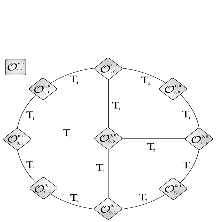
Figure 4.3: Interrelation of various operators via clustering. In this figure we use the abbreviations ${T_{1}\equiv\mathcal{T}_{1,2\kappa+1\leq l}^{\lambda}}$, ${T_{2}\equiv\mathcal{T}_{1,2\kappa+1\leq l}^{-\lambda}}$, ${T_{3}\equiv\mathcal{T}_{n-2\kappa<m,n}^{\lambda}}$, ${T_{4}\equiv\mathcal{T}_{n-2\kappa<m,n}^{-\lambda}}$. We also drop the 2s and 2t in the subscripts of the ${\mathcal{O}}$’s. The ${T_{i}}$ on the links operate in both directions.

4.7.1 The energy momentum tensor

As we observed from our previous discussion the solution $F_{2,2}^{1,1}$ is rather special. In fact this solution is part of the expression (4.84), which was identified as the trace of the energy momentum tensor

$$Q^{\Theta|2s+2,2t+2}=i^{s(2t+3)}e^{-(t+1)\sigma}\sigma_{1}\bar{\sigma}_{1}F_{2s+2,2t+2}^{1,1}\,\,.$$ (4.126)

The pre-factor $\sigma_{1}\bar{\sigma}_{1}$ will, however, alter the cluster property. The leading order behaviour reads now

$$\mathcal{T}_{1,\kappa\leq 2s}^{\pm\lambda}F^{\Theta|2s,2t}\sim\mathcal{T}_{n+1-\kappa<2t,n}^{\pm\lambda}F^{\Theta|2s,2t}\sim e^{\lambda(1-\kappa/2)}\,\,.$$ (4.127)

We observe that still in most cases the shifted expressions tend to zero, unless $\kappa=1$ for which it tends to infinity as a consequence of the introduction of the $\sigma_{1}\bar{\sigma}_{1}$. There is now also the interesting case $\kappa=2$, for which the $\lambda$-dependence drops out completely. Considering this case in more detail we find

$$\mathcal{T}_{1,2}^{\pm\lambda}F^{\Theta|2s,2t} \sim F^{\Theta|2,0}F^{\Theta|2s-2,2t}\times\QATOPD\{.{\frac{\sigma_{1}(x_{2s+1},\ldots,x_{2s+2t})}{\sigma_{1}(x_{3},\ldots,x_{2s+2t})}}{\frac{\bar{\sigma}_{1}(x_{2s+1},\ldots,x_{2s+2t})}{\bar{\sigma}_{1}(x_{3},\ldots,x_{2s+2t})}}$$ (4.128)

$$\mathcal{T}_{n+1-\kappa,n}^{\pm\lambda}F^{\Theta|2s,2t} \sim F^{\Theta|2s,2t-2}F^{\Theta|0,2}\times\QATOPD\{.{\frac{\sigma_{1}(x_{1},\ldots,x_{2s})}{\sigma_{1}(x_{1},\ldots,x_{2s+2t-2})}}{\frac{\bar{\sigma}_{1}(x_{1},\ldots,x_{2s})}{\bar{\sigma}_{1}(x_{1},\ldots,x_{2s+2t-2})}}\,.$$ (4.129)

Note that unless $s=1$ in (4.128) or $t=1$ in (4.129) the form factors do not “purely” factorise into known form factors, but in all cases a parity breaking factor emerges.

We now turn to the cases $\kappa=2s$ or $\kappa=2t$ for which we derive

$$\mathcal{T}_{1,2s}^{\pm\lambda}F^{\Theta|2s,2t}\sim\mathcal{T}_{n+1-2t,n}^{\pm\lambda}F^{\Theta|2s,2t}\sim e^{\lambda(2-t-s)}\,\,.$$ (4.130)

We observe that once again in most cases these expressions tend to zero. However, we also encounter several situations in which the $\lambda$-dependence drops out altogether. It may happen whenever $t=2$, $s=0$ or $s=2$, $t=0$, which simply expresses the relativistic invariance of the form factor. The other interesting situation occurs for $t=1$, $s=1$. Choosing temporarily (in general we assume $m_{-}=m_{+}$) $H_{2}^{\Theta|0,2}=2\pi m_{-}^{2}$ , $m=m_{-}=m_{+}e^{2G/\pi}$, we derive in this case

$$\mathcal{T}_{1,2}^{\lambda}F_{4}^{\Theta|2,2}=\frac{F_{2}^{\Theta|2,0}F_{2}^{\Theta|0,2}}{2\pi m^{2}}\,\,.$$ (4.131)

In general when shifting the first $2s$ or last $2t$ rapidities we find the following factorization

$$\mathcal{T}_{1,2s}^{\pm\lambda}F^{\Theta|2s,2t}\sim\mathcal{T}_{n+1-2t,n}^{\pm\lambda}F^{\Theta|2s,2t}\sim\text{ }F^{\Theta|2s,0}F^{\Theta|0,2t}\,\,.$$ (4.132)

This equation holds true when keeping in mind that the r.h.s. of this equation vanishes once it involves a form factor with more than two particles. Note that only in these two cases the form factors factorise “purely” into two form factors without the additional parity breaking factors as in (4.128) and (4.129).

4.8 Computing the Virasoro central charge

Having computed all form factors of the energy momentum tensor (see section 4.5.1), we are in the position to evaluate explicitly (4.33). We can now collect all the factors entering in the form factors $F_{n}^{\Theta|\mu_{1}\cdots\mu_{n}}$, namely the constants given by (4.75) the $Q$’s presented in (4.84) and the part coming from the minimal form factors, as presented in the general ansatz (4.56). The 2-particle contribution is given by (4.81) and for the 4-particle form factor we obtain,

$$F_{4}^{\Theta|++--}=\frac{-\pi m^{2}(2+\sum_{i<j}\cosh(\theta_{ij}))}{2\cosh(\theta_{12}/2)\cosh(\theta_{34}/2)}\prod_{i<j}\tilde{F}_{\text{min}}^{\mu_{i}\mu_{j}}(\theta_{ij}).$$ (4.133)

Notice that the $\sigma$-dependence is “hidden” in the minimal form factors (4.62). All the explicit expressions of the 6-particle form factors of the energy momentum tensor for $\sigma=0$ can be found in appendix B. The results obtained for the central charge are,

$$\Delta c^{(2)}=1,\qquad\Delta c^{(4)}=1.197...,\qquad\Delta c^{(6)}=1.199\ldots\,,\quad\text{for }\sigma<\infty,$$ (4.134)

where in the notation $\Delta c^{(n)}$, the superscript $n$ indicates the upper limit in (4.33) namely, when carrying out the sum (4.33), contributions until the $n$-particle form factor have been taken into account. Thus, the expected value of $c=6/5=1.2$ is well reproduced. Apart from the 2-particle contribution $\Delta c^{(2)}$, in which case the calculation can be performed analytically

$$\Delta c^{(2)}=\frac{3}{2}\int\limits_{-\infty}^{\infty}d\theta\frac{{|F_{\text{mim}}^{++}(2\theta)|}^{2}}{({\cosh\theta})^{4}}=\frac{3}{2}\int\limits_{-\infty}^{\infty}d\theta\Bigg{(}\frac{{\tanh\theta}}{{\cosh\theta}}\Bigg{)}^{2}=1,$$ (4.135)

the integrals in (4.33) have been computed directly via a brute force Monte Carlo integration. Typical standard deviations we achieve correspond to the order of the last digit we quote. Taking into account that, in the limit $\sigma\rightarrow\infty$ the only non-vanishing form factors of the energy momentum tensor are $F_{2}^{\Theta|\pm\pm}$ (see section 4.5.1), we obtain for the central charge

$$\lim_{\sigma\rightarrow\infty}\Delta c=1,$$ (4.136)

as we expected, since according to (4.55), in the limit $\sigma\rightarrow\infty$ we are left with a system of two non-interacting free fermions.

In short, the main outcome of this section is that the calculation of the ultraviolet Virasoro central charge associated to the $SU(3)_{2}$-HSG model in the context of the form factor analysis by means of Zamolodchikov’s $c$-theorem (4.33) provides a result which is in complete agreement with the S-matrix proposal [51] and with the physical picture obtained in chapter 3 through a TBA-analysis. However, we shall confirm in the next section that a form factor study can provide more information about the underlying CFT apart from its Virasoro central charge. In particular, we might be able to identify the ultraviolet conformal dimensions of those local operators for which at least the first non-vanishing form factors are known. Conversely, in the context of the TBA it remains, an open question how to identify the operator content. As we showed in chapter 3, it is sometimes possible to determine at least the dimension of the perturbing operator, despite the fact that the reason is unclear, by investigating periodicities in the so-called $Y$-systems [139], but no information about other local operators is available.

4.9 Identifying the operator content

Having solved Watson’s and the residue equations one has still little information about the precise nature of the operator corresponding to a particular solution. There exist, however, various non-perturbative (in the standard coupling constant sense) arguments which provide this additional information and which we now wish to exploit for the model at hand. Basically, all these arguments rely on the assumption that the superselection sectors of the underlying conformal field theory remain separated after a mass scale has been introduced. We will therefore first have a brief look at the operator content of the $G_{k}/U(1)^{\ell}$-WZNW coset models and attempt thereafter to match them with the solutions of the form factor consistency equations. For these theories the different conformal dimensions in the model can be parameterised by two quantities [59, 61]: a highest dominant weight $\Lambda$ of level smaller or equal to $k$ and its corresponding lower weights $\lambda$

$$\Delta(\Lambda,\lambda)=\frac{(\Lambda\cdot(\Lambda+2\rho))}{2(k+h)}-\frac{(\lambda\cdot\lambda)}{2k}\,\,.$$ (4.137)

The lower weight $\lambda$, may be constructed in the usual fashion (see e.g. [180]): Consider a complete weight string $\lambda+n\alpha,\ldots,\lambda,\ldots,\lambda-m\alpha$, that is all the weights obtained by successive additions (subtractions) of a root $\alpha$ from the weight $\lambda$, such that $\lambda+(n+1)\alpha$ ($\lambda-(m+1)\alpha$) is not a weight anymore. It is then a well known fact that the difference between the two integers $m,n$ is $m-n=\lambda\cdot\alpha$ for simply laced Lie algebras. This means starting with the highest weight $\Lambda$, we can work our way downwards by deciding after each subtraction of a simple root $\alpha_{i}$ whether the new vector, say $\chi$, is a weight or not from the criterion $m_{i}=n_{i}+\chi\cdot\alpha_{i}>0$. With the procedure just outlined we obtain all possible weights of the theory

In (4.137) $h$ is the Coxeter number of $G$ and $\rho$ is the Weyl vector which is defined as (see for instance [101])

$$\rho=\frac{1}{2}\sum_{\alpha>0}\alpha=\sum_{i=1}^{\ell}\lambda_{i},$$ (4.138)

i.e. half the sum over the positive roots or, equivalently, the sum over all fundamental weights, $\lambda_{i}$. Denoting the highest root of $G$ by $\psi$, the conformal dimension related to the adjoint representation $\Delta(\psi,0)$ is of special interest since it corresponds to the one of the perturbing operator which leads to the massive HSG-models. Taking the square length of $\psi$ to be $2$ and recalling the well known fact that the height of $\psi$, that is ht($\psi$), is the Coxeter number minus one, such that $(\psi\cdot\rho)=ht(\psi)=h-1$, it follows that $\mathcal{O}^{\Delta(\psi,0)}$is an operator with conformal dimension $\Delta(\psi,0)=h/(k+h)$, which is precisely the expression of the conformal dimension of the perturbing field [49]. Remarkably, the latter conformal dimension is obtained for a single combination of weights $(\Lambda,\lambda)$. Notice that, with the procedure described in the above paragraph it may happen that a weight corresponds to more than one linearly independent weight vector, such that the weight space may be more than one-dimensional. However, we will not take the multiplicities of the $\lambda$-states into account in this case and leave a more detailed study of this issue for the next chapter (see section 5.5). For $SU(3)_{2}$ the expression (4.137) is easily computed and since we could not find the explicit values in the literature we report them for reference in table 4.2.

$\lambda\backslash\Lambda$	$\lambda_{1}$	$\lambda_{2}$	$\lambda_{1}+\lambda_{2}$	$2\lambda_{1}$	$2\lambda_{2}$
$\Lambda$	$1/10$	$1/10$	$1/10$	$0$	$0$
$\Lambda-\alpha_{1}$	$1/10$	$*$	$1/10$	$1/2$	$*$
$\Lambda-\alpha_{2}$	$*$	$1/10$	$1/10$	$*$	$1/2$
$\Lambda-\alpha_{1}-\alpha_{2}$	$1/10$	$1/10$	$3/5$	$1/2$	$1/2$
$\Lambda-2\alpha_{1}$	$*$	$*$	$*$	$0$	$*$
$\Lambda-2\alpha_{2}$	$*$	$*$	$*$	$*$	$0$
$\Lambda-2\alpha_{1}-\alpha_{2}$	$*$	$*$	$1/10$	$1/2$	$*$
$\Lambda-\alpha_{1}-2\alpha_{2}$	$*$	$*$	$1/10$	$*$	$1/2$
$\Lambda-2\alpha_{1}-2\alpha_{2}$	$*$	$*$	$1/10$	$0$	$0$

Table 4.2: Conformal dimensions for ${\mathcal{O}^{\Delta(\Lambda,\lambda)}}$ in the ${SU(3)_{2}}/{U(1)^{2}}$-coset model. The ‘ * ’ indicate those cases for which the corresponding weight ${\lambda_{i}}$ does not arise as lower weight of $\Lambda$.

Turning now to the massive theory and once the spinless character of the operators (4.7) has been taken into account via (4.59), a crude constraint which gives a first glimpse at possible solutions to the form factor consistency equations based on their asymptotics is provided by the bound [161], which we presented at the beginning of this chapter ( 4.8) and referred to also as property 6 of the form factors.

It is useful to introduce at this point some new notation in addition to the useful abbreviation (4.9) we have extensively used in preceding sections. In the same spirit, we will use now the notation $[\,\,\,]_{\pm}$ when we take the limit in the variable $x_{i}$ related to the particle species $\mu_{i}=``\pm"$, respectively. For the different solutions we constructed, we reported the asymptotic behaviours in table 4.1. Notice that, assuming each of the 12 admissible solutions presented in table 4.1 has a counterpart in the underlying conformal field theory whose conformal dimension is contained in table 4.2, the asymptotic behaviours presented also in table 4.1 are always compatible with the bound (4.8), irrespectively of which of the conformal dimensions in 4.2 is the one associated to the operator at hand.

Being in a position in which we already anticipate the conformal dimensions in table 4.2, the bound (4.8) will severely restrict the possible inclusion of factors like $\sigma_{1},\bar{\sigma}_{1},\sigma_{1}^{-},\sigma_{1}^{+}$ and therefore the amount of different solutions to the recursive equations (4.71). Recall that it was stated in section 4.5 that factors of the type above mentioned may always be added to any of our solutions of table 4.1, since they trivially satisfy the consistency equations.

4.9.1 $\Delta$-sum rules

We may now turn to the identification of the operator content of the $SU(3)_{2}$-HSG model by exploiting the second of the techniques anticipated in subsection 4.1.6: the $\Delta$-sum rule provided in [27]. Since in our model the $n$-particle form factors related to the energy momentum tensor are only non-vanishing for even particle numbers, we might only use the $\Delta$-sum rule (4.36) [27] for the operators $\mathcal{O}_{0,0}^{0,0}$, $\mathcal{O}_{0,2}^{0,1}$, $\mathcal{O}_{2,0}^{1,0}$ and $\mathcal{O}_{2,2}^{1,1}$, where the latter operator is plagued by one of the problems stated in subsection 4.1.6 namely, its lowest non-vanishing form factor is not the vacuum expectation value.

We will now compute the sum rule for the operators $\mathcal{O}_{0,0}^{0,0}$, $\mathcal{O}_{0,2}^{0,1}$, $\mathcal{O}_{2,0}^{1,0}$ up to the 6-particle contribution. The explicit expressions or the corresponding form factors, until the 8-particle contribution have been collected in appendix B. We commence with the two particle contribution which is always evaluated effortlessly. Noting that, as we saw in section 4.5.1 the 2-particle form factor is given by (4.81) and the fact that $\Delta_{ir}^{\!\!\mathcal{O}}$ is zero in a purely massive model, the two particle contribution acquires the particular simple form

$$(\Delta^{\!\!\mathcal{O}})^{(2)}=\frac{i}{4\pi\left\langle\mathcal{O}\right\rangle}\int\limits_{-\infty}^{\infty}d\theta\frac{\tanh\theta}{\cosh\theta}\left(F_{2}^{\mathcal{O}|++}(2\theta)\right)^{*}\,\,\,.\,$$ (4.139)

Using now the explicit expressions for the two-particle form factors (B.4), we immediately find

$$(\Delta^{\!\!\mathcal{O}_{0,0}^{0,0}})^{(2)}=(\Delta^{\!\!\mathcal{O}_{0,2}^{0,1}})^{(2)}=(\Delta^{\!\!\mathcal{O}_{2,0}^{1,0}})^{(2)}=1/8\,\,\,.$$ (4.140)

Recall that, in the limit $\sigma\rightarrow\infty$ performed in section 4.5.1 we obtained two copies of the thermally perturbed Ising model for which the 2-particle form factor (4.81) is the only non-vanishing one related to the energy momentum tensor. Hence, in this limit, the sum over all particle types in (4.37) will receive only contributions from terms involving particles of the same type or, in other words, only the 2-particle contribution will occur. Consequently there will be two equal contributions, namely 1/16 from $F_{2}^{\mathcal{O}|++}$ and 1/16 from $F_{2}^{\mathcal{O}|--}$, such that the operator $\mathcal{O}_{0,0}^{0,0}$ plays the role of the disorder operator, as we expected.

To distinguish the operators $\mathcal{O}_{0,0}^{0,0}$, $\mathcal{O}_{0,2}^{0,1}$, $\mathcal{O}_{2,0}^{1,0}$ from each other we have to proceed to higher particle contributions. At present there exist no analytical arguments for this and we therefore resort to a brute force numerical computation.

Denoting by $(\Delta^{\!\!\mathcal{O}})^{(n)}$ the contribution up to the $n$-th particle form factor, our numerical Monte Carlo integration yields

$$\qquad(\Delta^{\!\!\mathcal{O}_{0,0}^{0,0}})^{(4)} = 0.0987\qquad(\Delta^{\!\!\mathcal{O}_{0,0}^{0,0}})^{(6)}=0.1004,$$ (4.141)

$$\qquad(\Delta^{\!\!\mathcal{O}_{0,2}^{0,1}})^{(4)} = 0.0880\qquad(\Delta^{\!\!\mathcal{O}_{0,2}^{0,1}})^{(6)}=0.0895,$$ (4.142)

$$\qquad(\Delta^{\!\!\mathcal{O}_{2,0}^{1,0}})^{(4)} = 0.0880\qquad(\Delta^{\!\!\mathcal{O}_{2,0}^{1,0}})^{(6)}=0.0895\,\,.$$ (4.143)

We shall be content with the precision reached at this point, but we will have a look at the overall sign of the next contribution. From the explicit expressions of the 8-particle form factors we see that for $\mathcal{O}_{0,0}^{0,0}$ the next contribution will reduce the value for $\Delta$. For the other two operators we have several contributions with different signs, such that the overall value is not clear a priory. In this light, we conclude that the operators $\mathcal{O}_{0,0}^{0,0}$, $\mathcal{O}_{0,2}^{0,1}$, $\mathcal{O}_{2,0}^{1,0}$ all possess conformal dimension $1/10$ in the UV-limit. Unfortunately, the values for the latter two operators do not allow such a clear-cut deduction as for the first one. Nonetheless, we base our statement on the knowledge of the operator content of the conformal field theory and confirm them also by elaborating directly on (4.35) and (4.22).

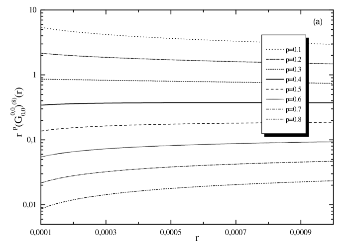
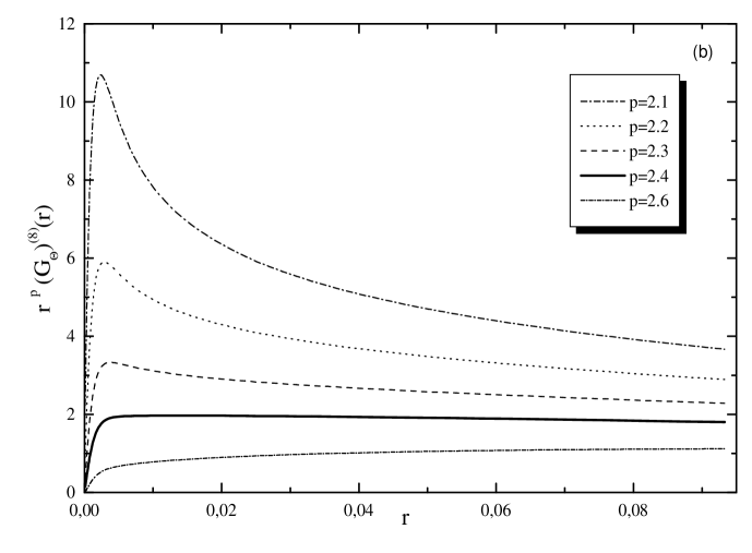
Figure 4.4: (a) Rescaled correlation function ${G_{0,0}^{0,0}(r):=\left\langle\mathcal{O}_{0,0}^{0,0}(r)\mathcal{O}_{0,0}^{0,0}(0)\right\rangle/{\langle\mathcal{O}_{0,0}^{0,0}\rangle}^{2}}$ summed up to the eight particle contribution as a function of $r$. (b) Rescaled correlation function ${(G_{\hat{\Theta}})^{(8)}(r):=\left\langle\hat{\Theta}(r)\hat{\Theta}(0)\right\rangle}$ summed up to the eight particle contribution as a function of ${r}$.

4.9.2 ${\Delta}$ from correlation functions

In the light of the results of the previous section, it is clear we can not use the $\Delta$-sum rule for a large class of operators of our model. Therefore we may resort to the study of the UV-behaviour of the two-point functions (4.35), as explained in subsection 4.1.6. We start by not assuming anything about the conformal dimension of the operator $\mathcal{O}$ and multiply its two-point correlation function (4.22) by $r^{p}$ with $p$ being some arbitrary power. Once this combination behaves as a constant in the vicinity of $r=0$ we take this value as the first non-vanishing three-point coupling divided by the vacuum expectation value of $\mathcal{O}$ and $p/4\,$as its conformal dimension. This means even without knowing the vacuum expectation value we have a rationale to fix $p$, but we can not determine the first term in (4.34 ). Figure 4.4 (a) exhibits this analysis for the operator $\mathcal{O}_{0,0}^{0,0}$ up to the $8$-particle contribution and we conclude from there that its conformal dimension is $1/10$.

The result of the same type of analysis for the energy momentum tensor is depicted in figure 4.4 (b), from which we deduce the conformal dimension $3/5$. Recalling that the energy momentum tensor is proportional to the dimension of the perturbing field [163] this is precisely what we expected to find.

Furthermore, we observe that the relevant interval for $r$ differs by two orders of magnitude, which by taking the upper bound for the validity of (4.35) into account should amount to $C_{\frac{1}{10}\frac{1}{10}0}C_{\frac{3}{5}\frac{3}{5}\frac{1}{10}}/(C_{\frac{3}{5}\frac{3}{5}0}C_{\frac{1}{10}\frac{1}{10}\frac{1}{10}})\sim\mathcal{O}(10^{-2})$. Since to our knowledge these quantities have not been computed from the conformal side, this inequality can not be double checked at this stage.

In figure 4.5 we also exhibit the individual $n$-particle contributions to the energy momentum tensor correlation function. Excluding the two particle contribution, these data also confirm the proportionality of the $n$-th term to ($\log(r))^{n}$. It is also interesting to notice that for small $r$ the 4-, and 6-particle contributions are higher than the 2-particle one which confirms the need of adding more and more terms in this region and the convenience of a more rigorous investigation of the convergence of the series (4.22).

We have carried out similar analysis for the other solutions we have constructed and report our findings in table 4.1. We observe that the combination of the vacuum expectation value times the three-point coupling for these operators differ, which is the prerequisite for unraveling the degeneracy.

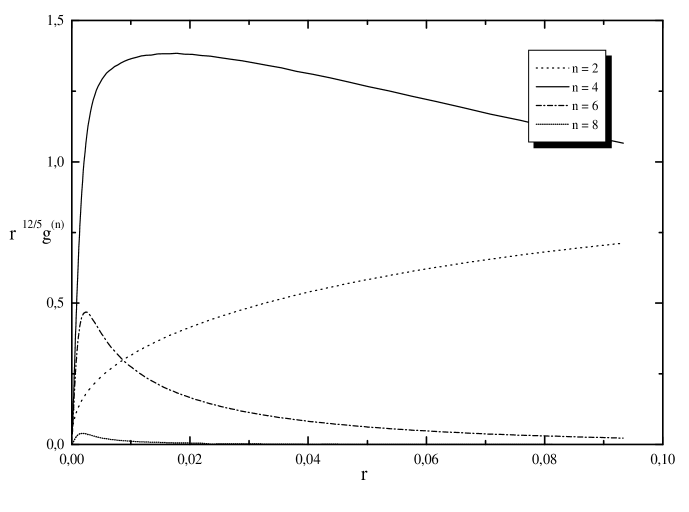
Figure 4.5: Rescaled individual $n$-particle contribution ${g^{(n)}(r)}$ to the correlation function of $\hat{\Theta}$ as a function of ${r}$.

4.10 RG-flow with unstable particles

Renormalisation group methods have been developed originally [181] to carry out qualitative analysis of regions of quantum field theories which are not accessible by perturbation theory in the coupling constant. Having computed in section 4.1.5 the ultraviolet Virasoro central charge associated to the $SU(3)_{2}$-HSG model and confirmed its consistence with the result achievable in the thermodynamic Bethe ansatz context (see section 3.3.2), we wish now to confirm and refine the physical picture emerging from the TBA-analysis by means of the former methods.

Recall that, in the TBA-context, the relative mass scales between the unstable and stable particles and the stable particles themselves were investigated by computing the finite size scaling function $c(r,\sigma)$. For this function a “staircase” behaviour (see figure 3.3) was observed. Such behaviour allowed a very interesting physical picture which we summarise now:

i)  In the UV-limit, when the temperature is very high all the particles of the model (for $\sigma$ finite) have masses much lower than the present energy scale and therefore all of them contribute to the total effective central charge reproducing the expected value $6/5$.

ii)  As soon as the scaling parameter $r$ becomes higher or, in other words, the temperature is lower we may reach an energy scale much lower than the mass of the unstable particle so that it can not be formed anymore. Hence, we are left with two non-interacting stable particles which give a contribution of 1/2 each to the scaling function. Being the mass of the unstable particle determined by the value of the resonance parameter $\sigma$ as explained in subsection 3.3.2 of chapter 3, such a “decoupling” will take place at different energy scales for different values of $\sigma$.

iii)  If the masses of these two stable particles are taken to be very different, eventually an energy scale for which only one of these particles can be produced may be reached and the corresponding scaling function flows to the value 1/2.

iv) Finally, in the infrared limit the scaling function tends to zero for purely massive QFT’s.

It is interesting to notice that the former physical picture required in the TBA-analysis the introduction of a parameter $r^{\prime}=\frac{r}{2}e^{\sigma/2}$ familiar from the discussion of the massless scattering [126]. This parameter which had only a formal meaning in the TBA-context arises naturally in the renormalisation group context, supporting the interpretation of this sort of flows as massless flows.

Recall that, for the $SU(3)_{2}$-HSG model the resonance pole $\theta_{R}=\mp\sigma-i\pi/2$ has an imaginary part $\bar{\sigma}=\pi/2$ so that, for arbitrary resonance parameter $\sigma$ one can deduce from (4.42), (4.43) that the condition $M_{\tilde{u}}\gg\Gamma_{\tilde{u}}$ is not fulfilled. However, as indicated in section 2.3, this condition only helps for a clearer identification of the mass parameter. For the HSG-models this condition starts to hold when the level is large, which indicates that $M_{\tilde{u}}\gg\Gamma_{\tilde{u}}$ just in the semi-classical regime [50, 51]. However, since we are not considering here the semi-classical regime, the interpretation of the flows observed as the trace of the presence of unstable particles in the model is not contradictory with the fact that the mentioned inequality does not hold for the model at hand.

Let us now analyse (4.49), (4.50) and (4.45) for the $SU(3)_{2}$-HSG model. As usual, we carry out the integrals by means of a Monte Carlo computation. For $c(r_{0})$ we take contributions up to the 4-particle form factor into account, namely the form factors (4.81) and (4.133), and display our results in figure 4.6.

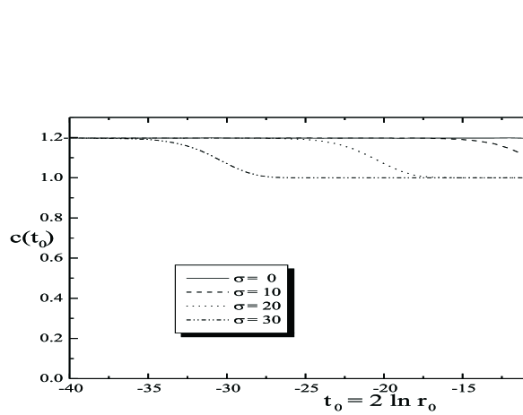
Figure 4.6: Renormalisation group flow for the Virasoro central charge ${c(r_{0})}$ for various values of the resonance parameter $\sigma$.

Following the renormalisation group flow from the ultraviolet to the infrared, figure 4.6 illustrates the flow from the $SU(3)_{2}/U(1)^{2}$- to the $SU(2)_{2}/U(1)\otimes SU(2)_{2}/U(1)$-coset, or in other words, from the values $c=6/5$ to the value $c=1/2+1/2=1$, when the unstable particle becomes massive. This confirms qualitatively the previous observation of the TBA analysis which we recalled at the beginning of this section and admits an entirely analogue physical explanation. Consequently, figures 4.6 and 3.3 are hardly distinguishable, despite the fact that both functions are different.

Although for the $SU(3)_{2}$-HSG model it is not possible to evaluate analytically either the finite size scaling function nor the Zamolodchikov $c$-function, one can realise that these two functions are different by direct comparison of figures 4.6 and 3.3. However, one could think this direct comparison is not quite reliable in our case since, for example, when evaluating (4.49) we are only taking terms up to the 4-particle contribution. In order to convince oneself that these two functions are indeed different one can look at a simpler model like the free fermion, for which both the finite size scaling function [116] and the $c$-function [27] have been obtained analytically and admit expressions in terms of Bessel functions. These analytical expressions, found in [116] and [27] respectively, show that the finite size scaling function and $c$-function are clearly different.

As we said, we also wish to analyse (4.45) for the $SU(3)_{2}$-HSG model in order to give a physical interpretation to our numerical results depicted in Fig. 4.6. Taking the mass scales of the stable particles to be the same, i.e. $m_{+}=m_{-}=m$ we want to compute now, for different choices of the resonance parameter $\sigma$, the values of the RG-parameter, $t_{u}$, at which the unstable particle becomes effectively massive (see paragraph before Eq. (4.48)). As we can see in Fig. 4.6, the flow between the two cosets is smooth and takes place over some range of $t_{0}$. For this reason we have to select one particular point $t_{u}$ in the mentioned range. As already indicated in general in subsection 4.1.7, it is convenient to identify $t_{u}$ as the point at which $c(t_{0})$ is half the difference between the two coset values of $c$. Indeed we find

$$(t_{u},\sigma)\approx(-30.8,30),(-20.8,20),(-10.8,10).$$ (4.144)

It is clear from Fig. 4.6 that, since the overall shape of the curves between two values of $c$ is identical for different values of $\sigma$, any other value in the interval would lead to the same results in comparative considerations. Analogously to situation encountered for the stable particles, for the unstable particles the RG-flow is indeed achieved by $M_{\tilde{c}}\rightarrow r_{u}M_{\tilde{c}}$, where $t_{u}=2\ln r_{u}$, $M_{\tilde{c}}$ is the mass of the unstable particle given by Eq. (4.45) and the combination $M_{\tilde{c}}(t_{u},\sigma):=r_{u}M_{\tilde{c}}$ must be interpreted as the ‘effective’ mass of the unstable particle with respect to the RG-group energy scale.

Actually, according to Eq. (4.45), and taking into account that, the values of $t_{u}$ given in (4.144) should be determined by the condition,

$$M_{u}(t_{u},\sigma)=r_{u}M_{\tilde{c}}\approx m\Rightarrow\frac{1}{\sqrt{2}}\,e^{(|\sigma|+t_{u})/2}\approx 1,$$ (4.145)

which just expresses the outlined assertion that the unstable particle starts ‘contributing’ to the value of the $c$-function or equivalently, can be excited, when its associated mass $M_{\tilde{c}}$ is of order $m/r_{u}$, that is, the energy scale fixed by the RG-parameter. The outcome of the evaluation of (4.145) for the values (4.144) is however $0.47$ instead of 1. Nonetheless, the latter result should not be taken too literally since the point $t_{u}$ is only chosen because it can be easily fixed.

For the evaluation of the scaled conformal dimension (4.50) we proceed similarly. For the solutions corresponding to the operators ${\cal O}_{0,0}^{0,0}$, ${\cal O}_{0,2}^{0,1}$ and ${\cal O}_{2,0}^{1,0}$, whose conformal dimension in the UV-limit was identified in section 4.9.1 to be $1/10$, we take up to the 6-particle form factors into account (see appendix B for their explicit expressions). For the former two operators our results are presented in figures 4.7 and 4.8.

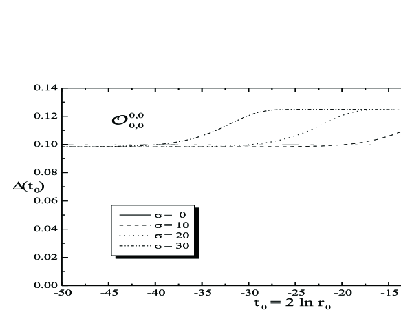
Figure 4.7: Renormalisation group flow for the conformal dimension ${\Delta(r_{0})}$ of the operator ${{\cal O}_{0,0}^{0,0}}$ for various values of the resonance parameter $\sigma$.

We observe that the conformal dimension of the operator ${\cal O}_{0,0}^{0,0}$ flows to the value $1/8$, which is twice the conformal dimension of the disorder operator $\mu$ in the Ising model. The factor $2$ is expected from the mentioned coset structure, i.e. we find two copies of $SU(2)_{2}/U(1)$. The nature of the operator is also anticipated, since by construction the form factors $F_{n}^{{\cal O}_{0,0}^{0,0}}$ of the $SU(3)_{2}$-HSG model coincide precisely with $F_{n}^{\mu}$ of the thermally perturbed Ising model when the number of particles of type “+ ” or “ - ” is zero. It is also clear that we could alternatively obtain (4.144) from the analysis of $\Delta(r_{0})$.

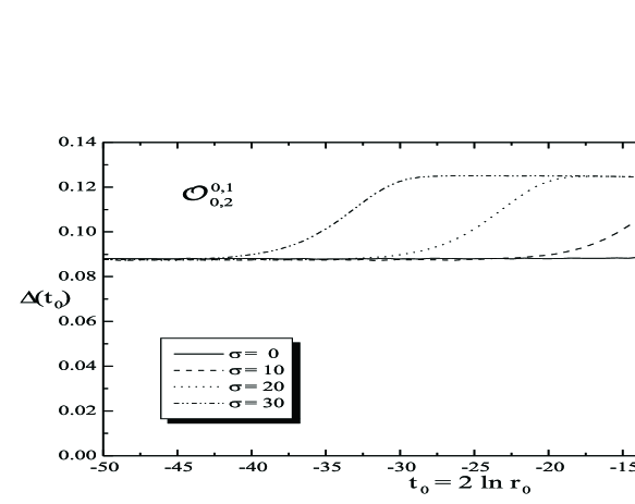
Figure 4.8: Renormalisation group flow for the conformal dimension ${\Delta(r_{0})}$ of the operator ${{\cal O}_{0,2}^{0,1}}$ for various values of the resonance parameter $\sigma$.

Despite the fact that the explicit expressions for the form factors of ${\cal O}_{0,2}^{0,1}$ and ${\cal O}_{2,0}^{1,0}$ differ (see appendix B) the values of $\Delta(r_{0})$ are hardly distinguishable and we therefore omit the plots for the latter case. We also note the previously observed fact, that the higher particle contributions for the latter operators are more important than for ${\cal O}_{0,0}^{0,0}$, which explains the fact that the starting point at the ultraviolet fixed point is not quite $0.1$ but $0.0880$ as observed in (4.143). The operators also flow to the value $1/8$, such that the degeneracy of the $SU(3)_{2}$-HSG model disappears surjectively when the unstable particle becomes massive.

In conclusion, the RG-flow of Zamolodchikov’s $c$-function and of the conformal dimensions of various operators, allows a clear physical interpretation which is in complete agreement with the interpretation of the “staircase” pattern observed for the scaling function computed in the TBA.

4.11 Summary of results and open problems

Concerning the main objective we addressed in this chapter, we draw the overall conclusion that the outcome of the form factor analysis for the $SU(3)_{2}$-HSG model confirms the physical picture obtained by means of the thermodynamic Bethe ansatz in chapter 3. The Virasoro central charge of the underlying CFT $(c=6/5)$ has been obtained by means of Zamolodchikov’s $c$-theorem [24] and qualitatively the same “staircase” behaviour [108] observed for the finite size scaling function (3.35) as a function of the energy scale in chapter 3 has been found for the renormalisation group flow of Zamolodchikov’s $c$-function as a function of the renormalisation group parameter $r_{0}$. In this context, the variable $me^{|\sigma|/2}$, originally introduced in [126] to describe the massless scattering, arises naturally through formula (4.45), which supports the idea, also present in the TBA-context, that the sort of flows observed, related to the presence of unstable particles in the spectrum, can be understood as massless flows.

In addition to the TBA-results, our form factor analysis allowed for the identification of, at least an important part of the operator content of the $SU(3)_{2}$-HSG model via the calculation of the corresponding ultraviolet conformal dimension of those operators for which all the $n$-particle form factors had been previously computed. In particular, the conformal dimension of the perturbing operator ($\Delta=3/5$) was obtained by studying the ultraviolet behaviour of the two-point function of the energy momentum tensor. In this light, it can be stated that solutions of the form factor consistency equations can be identified with operators in the underlying ultraviolet conformal field theory. In this sense one can give meaning to the operator content of the integrable massive model. Being the mentioned identification uniquely based on the values of the ultraviolet conformal dimensions there is the problem that once the conformal field theory is degenerate in this quantity, as it is the case for the model we investigated, the identification can not be carried out in a one-to-one fashion and therefore the procedure has to be refined. In principle this would be possible by including the knowledge of the three-point coupling of the conformal field theory and the vacuum expectation value into the analysis. The former quantities are in principle accessible by working out explicitly the conformal fusion structure, whereas the computation of the latter still remains an open challenge. In fact what one would like to achieve ultimately is the identification of the conformal fusion structure within the massive models. Considering the total number of operators present in the conformal field theory (see table 4.2), one still expects to find additional solutions, in particular the identification of the fields possessing conformal dimension $1/2$ is an outstanding problem.

With respect to the explicit calculation of conformal dimensions, technically we have confirmed that the sum rule (4.36) is clearly superior to the direct analysis of the correlation functions. However, it has also the inconvenient that in theories with internal symmetries, as the one at hand, it only applies for certain operators. It would therefore be highly desirable to develop arguments which also apply for theories with internal symmetries and possibly to resolve the mentioned degeneracies in the conformal dimensions.

As mentioned in several occasions throughout this chapter, the question of how to identify the operator content of a massive integrable quantum field theory is left unanswered in the TBA-context, apart from the identification of the conformal dimension of the perturbing field, sometimes related to the periodicity of the so-called $Y$-systems [139]. From that point of view, one can say that the form factor program provides more information about the underlying CFT than the TBA and therefore a more rigorous check of the S-matrix proposal [51]. In addition, our analysis contributes to the further development of the QFT associated to the HSG-models.

At the mathematical level, a closed formula (4.79) for all $n$-particle form factors associated to a large class of operators has been found. This formula is given in terms of building blocks which can be expressed both as determinants whose entries are elementary symmetric polynomials (4.77) or by means of an integral representation (4.80). However, it remains an open question, whether the general solution procedure presented in section 4.4 can be generalised to the degree that determinants of the type (4.77) will serve as generic building blocks of form factors. It remains also for us to be understood how an integral representation of the type (4.80) might be used in practise, for instance, to formulate rigorous proofs of the type presented in section 4.6. In general, it would be very interesting to exploit this integral representation for the same purposes we have used the determinant formula (4.77) namely, providing general proofs or analysing the cluster property. Another interesting open problem is to find out the precise relationship between this integral representation, which involves contour integral in the $x=e^{\theta}$-plane, and the integral representation used for instance in [155] which involved contour integrals in the $\theta$-plane.

It would be also desirable to put further constraints on the solutions to the form factor consistency equations by means of other arguments, that is exploiting the symmetries of the model, formulating quantum equations of motion, possibly performing perturbation theory etc…

Concerning the momentum space cluster property, our analysis also provides remarkable results. It has been proven in section 4.7 that it does not only constrain the solutions to the form factor consistency equations but also serves as a construction principle to obtain new solutions. In particular, for the operators itemized in table 4.1 we have verified that starting with the solutions for any of the first 9 operators one could re-construct all the others, obtained initially by solving the recursive equations (4.71). Clearly, it would be very interesting to develop arguments which allowed us to reach a level of understanding of this property similar to the one we have for the rest of the form factor consistency equations [22, 153, 152, 154, 155].

Regarding the RG-analysis carried out in section 4.10, we have recovered the TBA-picture extracted from the computation of the finite size scaling function. We find that the $c$-function defined by means of Zamolodchikov’s $c$-theorem encodes the same physical information than the scaling function or Casimir energy computed in the TBA. Therefore, it would be extremely desirable to elaborate on the precise relationship between these two functions which providing the same physical information are however different. Being the finite size scaling function and Zamolodchikov’s $c$-function defined in such, at first sight, disconnected contexts, the nature of such relationship is not clear a priori. Also the relation to the intriguing proposal in [182] of a renormalisation group flow between Virasoro characters remains unclarified. It is also relevant the fact that, although in the “excited” TBA-framework [25, 26] the conformal dimensions of certain fields of the underlying CFT different from the perturbing field can be identified, the analogue of $\Delta(r_{0})$ still needs to be found in the TBA as well as in the context of [182].

To finish this chapter, it is worth emphasising that, apart from providing a double-check of the results of our TBA-analysis, the form factor program developed for the $SU(3)_{2}$-HSG model has also contributed to the general understanding of the form factor program itself in various aspects like, for instance, the finding of general solutions to recursive problems of the type (4.71), the identification of the operator content of a 1+1-dimensional massive integrable QFT or, the understanding of the momentum space cluster property (4.10) as a construction principle of new solutions to the form factor consistency equations. Concerning the physical picture presented for the $SU(3)_{2}$-homogeneous sine-Gordon model in [49, 50, 51], one can surely claim that it rests now on quite firm ground and it is now a challenge to extend the results of this chapter, to higher rank Lie groups. As a first step in this direction, a generalisation of the form factor construction and the renormalisation group analysis for all the $SU(N)_{2}$-HSG models shall be presented in the next chapter.

Chapter 5 Generalizing the form factor program to the ${SU(N)_{2}}$-HSG models.

For most integrable quantum field theories in 1+1 space-time dimensions it remains an open challenge to complete the entire bootstrap program, i.e. to compute the exact on-shell S-matrix, closed formulae for the $n$-particle form factors, identify the entire local operator content and in particular thereafter to compute the related correlation functions. In the previous chapter we investigated a particular model, the $SU(3)_{2}/U(1)^{2}$-homogeneous Sine-Gordon model [48, 49, 50, 63, 90] (HSG), for which this task was completed to a large extend. In particular, general formulae for the $n$-particle form factors related to a large class of local operators were provided. In order to understand the generic group theoretical structure of the $n$-particle form factor expressions and to provide further consistency checks of the S-matrix proposal [51] it is highly desirable to extend our analysis to higher rank Lie algebras as well as to higher level.

The extension of the form factor program to higher level is not straightforward since once $k>2$, stable bound states might be formed (see [51]). As a consequence, the corresponding form factors possess not only kinematical simple poles but also bound state poles, as indicates the so-called “bound state residue equation” [167] (see also section 4.1 of the previous chapter) and therefore, the mentioned equation has to be solved in addition to all the other form factor consistency equations [22, 153, 152, 154, 155]. As we have seen, the bound state residue equation establishes a recursive structure between the $(n+1)$- and $n$-particle form factor which we should solve in addition to the familiar recursive equations relating the $(n+2)$- and $n$-particle form factor, whose solution was already very intricate. On this light, we expect the form factor program to become much more complicated for models where stable bound states are present. Some of the simplest examples of models containing stable bound states are the Yang-Lee model [152] and the Bullough-Dodd model [183]. The spectrum of the latter model contains a single particle state, say $A$, which can be formed as bound state of itself in a scattering process of the type $A\times A\rightarrow A\rightarrow A\times A$. A closed formula for all $n$-particle form factors of the elementary field of the Bullough-Dodd model, and for particular values of the effective coupling constant was found in [158].

Consequently, we shall start the generalisation of the analysis performed for the $SU(3)_{2}$-HSG model by increasing the rank of the Lie algebra, that is, we intend to investigate the $SU(N)_{2}$-HSG models within the form factor context.

The results presented in this chapter might be found in [74]. Our analysis is organised as follows:

In section 5.1 we report the main characteristics of the $SU(N)_{2}$-HSG model. In particular the basic data characterising the corresponding underlying CFT, the scattering matrix and the stable and unstable particle content. Thereafter, in section 5.2 we start the form factor construction in the usual way, by providing a general ansatz for the form factor solutions. We derive the corresponding recursive equations and determine the minimal form factors. In section 5.3 we systematically construct all $n$-particle solutions to the form factor consistency equations. These solutions correspond to a large class of local operators, although they do not fulfill the entire operator content of the model. It turns out that these solutions involve the same sort of building blocks i.e, determinants whose entries are elementary symmetric polynomials, which we found in chapter 4. It is also possible to formulate a general proof for the $SU(N)_{2}$-solutions along the same lines pointed out in section 4.6. In section 5.4 we investigate the RG-flow of Zamolodchikov’s $c$-function [24], reproducing the physical picture expected for the HSG-models, namely the decoupling of the theory into two non-interacting systems whenever one of the resonance parameters becomes much larger than the energy scale considered. The same decoupling is also observed for the corresponding Virasoro central charge of the underlying CFT in the deep UV-limit. In section 5.5 we report the operator content in terms of primary fields of the underlying CFT of the $SU(4)_{2}$-HSG model. We also compute the conformal dimension of some operators present in any $SU(N)_{2}/U(1)^{N-1}$-WZNW coset theory as, for instance, the perturbing operator. In both cases we make use of the general formula derived in [59] for the conformal dimensions of primary fields of the $G_{k}$-parafermion theories. In subsection 5.5.1 we investigate the RG-flow of the conformal dimension of a certain local operator by means of the $\Delta$-sum rule [27] and identify its ultraviolet central charge in the limit when the renormalisation group parameter $r_{0}\rightarrow 0$. In subsection 5.5.2 we identify the conformal dimension of the perturbing operator in the $SU(4)_{2}$- and $SU(5)_{2}$-cases by investigating the UV-behaviour of the two-point function of the trace of the energy momentum tensor $\Theta$. Finally we report our main conclusions and point out some open questions in section 5.6.

5.1 The ${SU(N)_{2}}$-homogeneous sine-Gordon models.

The particularisation of the results presented in chapter 2 for the generality of the HSG models allows for viewing the $SU(N)_{2}$-HSG model as the perturbation of a gauged WZNW-coset $SU(N)_{2}/U(1)^{N-1}$ whose associated Virasoro central charge is given by

$$c_{SU(N)_{2}/U(1)^{N-1}}=\frac{N(N-1)}{(N+2)},$$ (5.1)

by means of an operator of conformal dimension

$$\Delta=\frac{N}{(N+2)}.$$ (5.2)

The theory possesses already a fairly rich particle content, namely $N-1$ asymptotically stable particles characterised by their mass scales $m_{i}$, $i=1,\cdots,N-1$ and $N-2$ unstable particles whose energy scale is characterised by the resonance parameters $\sigma_{ij}=-\sigma_{ji}$, $i,j=1,\cdots,N-1$. As found in [50, 51], the stable particles can be related in a one-to-one fashion to the vertices of the $SU(N)$-Dynkin diagram and one can associate to the link between vertex $i$ and $j$ the $N-2$ linearly independent resonance parameters $\sigma_{ij}$.

The physical picture provided in [48, 49, 50] and [51] for the homogeneous sine-Gordon models and checked in chapters 3 and 4 for the $SU(3)_{2}$-HSG model indicates that, once an unstable particle becomes extremely heavy the original coset decouples into a direct product of two cosets different from the original one in the following way

$$\lim\limits_{\sigma_{i,i+1}\rightarrow\infty}SU(N)_{2}/U(1)^{N-1}\equiv SU(i+1)_{2}/U(1)^{i}\otimes SU(N-i)_{2}/U(1)^{N-i-1}\,.$$ (5.3)

The latter equation means that, when investigating the renormalisation group flow of Zamolodchikov’s $c$-function, in a similar fashion we did for the $SU(3)_{2}$-HSG model, we expect to observe starting in the ultraviolet limit, a flow between the value (5.1) of the Virasoro central charge and the value obtained from the sum of the Virasoro central charges associated to the cosets arising on the r.h.s. of Eq. (5.3). Equivalently, when studying the RG-flow of the conformal dimension of any local operator of the $SU(N)_{2}$-HSG model computed by means of the $\Delta$-sum rule [27], we expect to identify the flow between the operator contents of the HSG models constructed as perturbations of the WZNW-cosets arising on the l.h.s. and r.h.s. of Eq. (5.3).

In other words, we may summarize the flow along the renormalisation group trajectory with increasing RG-parameter $r_{0}$ to cutting the related Dynkin diagrams at decreasing values of the $\sigma$’s. For instance taking $\sigma_{i,i+1}$ to be the largest resonance parameter at some energy scale the following cut takes place:

Resorting to the usual expressions for the coset central charge [102] of the WZNW-cosets (5.3), the decoupled system has the central charge

$$\lim\limits_{\sigma_{i,i+1}\rightarrow\infty}\!\!\!\!c_{SU(N)_{2}/U(1)^{N-1}} = c_{SU(i+1)_{2}/U(1)^{i}\otimes SU(N-i)_{2}/U(1)^{N-i-1}}=$$

$$c_{SU(i+1)_{2}/U(1)^{i}}+c_{SU(N-i)_{2}/U(1)^{N-i-1}} = N-5+\frac{6(N+5)}{(N+2-i)(3+i)}\,.$$ (5.4)

As an input necessary for the computation of form factors and correlation functions thereafter we must introduce now the exact scattering matrix proposed in [51] to describe the scattering theory of the $SU(N)_{2}$-HSG models. The two-particle S-matrix describing the scattering of two stable particles of type $i$ and $j$, with $1\leq i,j\leq N-1$ related to this model, as a function of the rapidity $\theta$, may be written as

$$S_{ij}(\theta)=(-1)^{\delta_{ij}}\left[c_{i}\tanh\frac{1}{2}\left(\theta+\sigma_{ij}-i\frac{\pi}{2}\right)\right]^{I_{ij}}\,.$$ (5.5)

Here, to make notation more compact, we have introduced the incidence matrix of the $SU(N)$-Dynkin diagram, denoted by $I$. This matrix is defined in terms of the Cartan matrix $K$ as $I=2-K$. In particular, for the $su(N)$ Lie algebra at hand we have

$$I_{ij}=\delta_{i,j-1}+\delta_{i,j+1}.$$ (5.6)

Both in (5.6) and in (5.5) we used the usual Kronecker delta defined as,

$$\delta_{ij}=\left\{\begin{array}[]{ll}0&\text{for}\,\,i\neq j,\\ 1&\text{for}\,\,i=j\end{array}\right.$$

The parity breaking which is characteristic for the HSG models and manifests itself by the fact that $S_{ij}\neq S_{ji}$, takes place through the resonance parameters $\sigma_{ij}=-\sigma_{ji}$ and the phases encoded in the colour value $c_{i}$. The latter quantity arises from a partition of the $SU(N)$-Dynkin diagram into two disjoint sets, which we refer to as “$+$” and “$-$”. We then associate the values $c_{i}=\pm 1$ to the vertices $i$ of the Dynkin diagram of $SU(N)$, in such a way that no two vertices related to the same set are linked together. These colour values $c_{i}$ provide a natural generalisation of the indices “$+$” and “$-$” we used in the previous chapter to label the two stable particles associated to the $SU(3)_{2}$-HSG model. They turn out to be also very useful aiming towards a generalisation of the form factor analysis performed for the latter model. Likewise we could simply divide the particles into odd and even, however, such a division would be specific to $SU(N)$ and the bi-colouration just outlined admits a generalization to other groups as well. The resonance poles in $S_{ij}(\theta)$ at $(\theta_{R})_{ij}=-\sigma_{ij}-i\pi/2$ may be understood in the usual Breit-Wigner fashion [89] as the trace of $N-2$ unstable particles as explained for instance in [14, 51] and chapter 2. Recall also that the mass of the unstable particle $M_{\tilde{c}}\,\$formed in the scattering between the stable particles $i$ and $j$ behaves as $M_{\tilde{c}}\sim me^{\left|\sigma_{ij}\right|/2}$, for $m$ to be the mass scale of the stable particles. This fact was observed both in the TBA- and the form factor analysis carried out in the previous chapters as well as in the original literature [51]. There are no poles present in the physical region of the imaginary axis, which indicates that no stable bound states may be formed and therefore the form factor construction does not require the use of the mentioned bound state residue equation. Hence, we shall follow the lines of the analysis performed in chapter 4.

Notice that the two-particle S-matrix (5.5) reduces to the S-matrix of the thermally perturbed Ising model whenever the interaction of particles of the same type is considered

$$S_{ii}(\theta)=-1.$$ (5.7)

This property will be widely exploited in the course of our form factor analysis for the same reasons argued before, namely it serves as a “seed” for the recursive problem relating the $(n+2)$- and $n$-particle form factor we have to solve in order to determine explicitly the form factors associated to any local operator of the $SU(N)_{2}$-HSG model.

It is also clear from the expression of the scattering matrix (5.5), that whenever a resonance parameter $\sigma_{ij}$ with $I_{ij}\neq 0$ (which always corresponds to $i\neq j$) goes to infinity, we observe for the corresponding S-matrix that

$$\lim_{\sigma_{ij}\rightarrow\infty}S_{ij}(\theta)=1$$ (5.8)

and consequently, we may view the whole system as consisting out of two sets of particles which only interact freely amongst each other. A physical consequence is that the unstable particle, whose mass behaved as $M_{\tilde{c}}\sim me^{\left|\sigma_{ij}\right|/2}$, for $m$ to be the mass scale of the stable particles, and was created in interaction process between these two theories before taking the limit, becomes so heavy that it can not be formed anymore at any energy scale. It can be easily deduced from (5.8) and (5.7) that in the case when all the resonance parameters tend to infinity or all the unstable particle become extremely heavy, we will deal with $N-1$ non-interacting copies of the thermally perturbed Ising model. Equivalently, when studying the renormalisation group flow of Zamoldchikov’s $c$-function we may reach an energy scale $r_{0}$, for which no formation of unstable particles is possible. Accordingly, the $c$- function will flow to the value $(N-1)/2$.

5.2 Recursive equations and minimal form factors

We are now in the position to compute the $n$-particle form factors related to this model, i.e. the matrix elements of a local operator ${\cal O}(\vec{x})$ located at the origin between a multi-particle in-state of particles (solitons) of species $\mu_{i}$, created by the vertex operators $V_{\mu_{i}}(\theta_{i})$, and the vacuum.

We proceed in the standard way by solving the form factor consistency equations [22, 153, 152, 154, 155]. For this purpose we extract explicitly, according to standard procedure, the singularity structure. Since no stable bound states may be formed during the scattering of two stable particles the only poles present are the ones associated to the kinematic residue equations, that is a first order pole for particles of the same type whose rapidities differ by $i\pi$. Therefore, we parameterise the $n$-particle form factors as

$$F_{n}^{{\cal O}|{\mathfrak{M}}(l_{+},l_{-})}(\theta_{1}\ldots\theta_{n})=H_{n}^{{\cal O}|{\mathfrak{M}}(l_{+},l_{-})}Q_{n}^{{\cal O}|{\mathfrak{M}}(l_{+},l_{-})}({\mathfrak{X})}{\mathfrak{\,}\!\!}\times\prod_{1\leq i<j\leq n}\frac{F_{\text{min}}^{\mu_{i}\mu_{j}}(\theta_{ij})}{\left(x_{i}^{c_{\mu_{i}}}+x_{j}^{c_{\mu_{j}}}\right)^{\delta_{\mu_{i}\mu_{j}}}}\,\,\,,$$ (5.9)

in clear analogy to the parameterisation (4.56) presented in section 4.4. Aiming towards a universally applicable and concise notation, it is convenient to collect the particle species $\mu_{1}\ldots\mu_{n}$ in form of particular sets

$${\mathfrak{M}_{i}}(l_{i}) = \{\mu\,|\,\mu=i\}$$ (5.10)

$${\mathfrak{M}_{\pm}}(l_{\pm}) = \bigcup_{i\in\pm}{\mathfrak{M}_{i}}(l_{i})$$ (5.11)

$${\mathfrak{M}}(l_{+},l_{-}) = {\mathfrak{M}_{+}}(l_{+})\cup{\mathfrak{M}_{-}}(l_{-}).$$ (5.12)

that is, we collect in ${\mathfrak{M}_{i}}(l_{i})$ a set of $l_{i}$ particles of the same type ‘$i$’ i.e., a set of $l_{i}$ particles associated to the same vertex $\alpha_{i}$ in the $SU(N)$-Dynkin diagram. Analogously, the sets ${\mathfrak{M}_{\pm}}(l_{\pm})$ collect the $l_{\pm}$ particles associated to vertices of the $SU(N)$-Dynkin diagram corresponding to $c_{i}=\pm 1$ respectively, according to the bi-colouration of the roots in the Dynkin diagram introduced in the previous section. We understand here that inside the sets ${\mathfrak{M}_{\pm}}$ the order of the individual sets ${\mathfrak{M}_{i}}$ is arbitrary. This simply reflects the fact that particles of different species but identical colour interact freely. However, ${\mathfrak{M}}$ is an ordered set since elements of ${\mathfrak{M}_{+}}$ and ${\mathfrak{M}_{-}}$ do not interact freely and w.l.g. we adopt the convention that particles belonging to the “$+$”-colour set come first. As usual, the $H_{n}$ are some overall constants and the $Q_{n}$ are polynomial functions depending on the variables $x_{i}=\exp\theta_{i}$ which are collected in the sets ${\mathfrak{X},}{\mathfrak{X}_{i},}{\mathfrak{X}_{\pm}}$ in a one-to-one fashion with respect to the particle species sets ${\mathfrak{M},}{\mathfrak{M}_{i},}{\mathfrak{M}_{\pm}}$. The functions $F_{\text{min}}^{\mu_{i}\mu_{j}}(\theta_{ij})$ are the minimal form factors introduced in section 4.3, which by construction contain no singularities in the physical sheet and solve Watson’s equations [22, 153] for two particles. For the $SU(N)_{2}$-HSG model they are found to be

$$F_{\text{min}}^{ij}(\theta)={({\cal N}_{c_{i}})}^{I_{ij}}\left(\sin\frac{\theta}{2i}\right)^{\delta_{ij}}e^{-I_{ij}\int\limits_{0}^{\infty}{{\frac{dt}{t}}}{\textstyle{\sin^{2}\left((i\pi-\theta\mp\sigma_{ij})\frac{t}{2\pi}\right)\over\sinh t\cosh t/2}}}\,,$$ (5.13)

where, the normalisation constants ${\cal N}_{c_{i}}$, are given by

$${\cal N}_{c_{i}}=2^{\frac{1}{4}}\exp\left(i\pi\frac{(1-c_{i}(1-\theta))}{4}-\frac{G}{4}\right)$$ (5.14)

and depend on the Catalan constant $G$. Notice the parallelism between (5.13) and equations (4.60), (4.62) in the previous chapter. Also the following asymptotic behaviours are very close to the ones presented in section 4.3

$$\lim\limits_{\sigma\rightarrow\infty}F_{\text{min}}^{\mu_{i}\mu_{i+1}}(\pm\theta)\sim e^{-\frac{\sigma_{i,i+1}}{4}},\qquad\qquad\left[F_{\text{min}}^{\mu_{i},\mu_{j}}(\theta_{ij})\right]_{i}=\frac{\delta_{c_{i},c_{j}}-\delta_{c_{i+1},0}\delta_{c_{j-1},0}}{2}.$$ (5.15)

were we used the abbreviation (4.9).

It is convenient also to introduce the notation

$$\tilde{F}_{\text{min}}^{ij}(\theta)=(e^{-c_{i}\theta/4}F_{\text{min}}^{ij}(\theta))^{I_{ij}},$$ (5.16)

The minimal form factors obey the functional identities

$$F_{\text{min}}^{ij}(\theta+i\pi)F_{\text{min}}^{ij}(\theta)=\left(-\frac{i}{2}\sinh\theta\right)^{\delta_{ij}}\left(\frac{i^{\frac{2-c_{i}}{2}}\,e^{\frac{\theta}{2}c_{i}}}{\cosh\left(\frac{\theta}{2}-\frac{i\,\pi}{4}\right)}\right)^{I_{ij}}.$$ (5.17)

Substituting the ansatz (5.9) into the kinematic residue equation , we obtain with the help of (5.17) a recursive equation for the overall constants for  $\mu_{i}\in{\mathfrak{M}_{+}}$

$$H_{n+2}^{{\cal O}|{\mathfrak{M}}(l_{+}+2,l_{-}{\mathfrak{)}}}=i^{\bar{l}_{i}}2^{2l_{i}-\bar{l}_{i}+1}e^{I_{ij}\sigma_{ij}l_{j}/2}H_{n}^{{\cal O}|{\mathfrak{M}(}l_{+},l_{-}{\mathfrak{)}}}\,\,{\mathfrak{\,}\,.}$$ (5.18)

We introduced here the numbers $\bar{l}_{i}=\sum_{\mu_{j}\in{\mathfrak{M}_{-}}}I_{ij}l_{j}$, which count the elements in the neighbouring sets of ${\mathfrak{M}_{i}}$.

The $Q$-polynomials have to obey the recursive equations

$$Q_{n+2}^{{\cal O}|{\mathfrak{M}}(2+l_{+},l_{-})}({\mathfrak{X}}^{xx}) = D_{\varsigma_{i}}^{2s_{i}+\tau_{i},2\bar{s}_{i}+\bar{\tau}_{i}}(\mathfrak{X}^{xx})Q^{{\cal O}|{\mathfrak{M}}(l_{+},l_{-})}{(\mathfrak{X})\,}\,\,\,$$ (5.19)

$$D_{\varsigma_{i}}^{2s_{i}+\tau_{i},2\bar{s}_{i}+\bar{\tau}_{i}}(\mathfrak{X}^{xx}) = \sum_{k=0}^{\bar{s}_{i}}x^{2s_{i}-2k+\tau_{i}+1-\varsigma_{i}}\sigma_{2k+\varsigma_{i}}(I_{ij}{\mathfrak{\hat{X}}}_{j})(-i)^{2s_{i}+\tau_{i}+1}\sigma_{2s_{i}+\tau_{i}}({\mathfrak{X}}_{i}).\,\,\,$$ (5.20)

For convenience we defined the sets ${\mathfrak{X}}^{xx}:=\{-x,x\}\cup{X}$, ${\mathfrak{\hat{X}}:=}ie^{\sigma_{i,i+1}}{\mathfrak{X}}$ and the integers $\zeta_{i}$ which are $0$ or $1$ depending on whether the sum $\vartheta+\tau_{i}$ is odd or even, respectively. $\vartheta$ is related to the factor of local commutativity [154] $\omega=(-1)^{\vartheta}=\pm 1$. As usual $\sigma_{k}(x_{1},\ldots,x_{m})$ is the $k$-th elementary symmetric polynomial. Furthermore, we used the sum convention $I_{ij}{\mathfrak{\hat{X}}}_{j}\equiv\mathop{\textstyle\bigcup}\sum_{\mu_{j}\in{\mathfrak{M}}}I_{ij}{\mathfrak{\hat{X}}}_{j}$ and parameterised $l_{i}=2s_{i}+\tau_{i}$, $\bar{l}_{i}=2\bar{s}_{i}+\bar{\tau}_{i}$ in order to distinguish between odd and even particle numbers.

Recall that, in the $SU(3)_{2}$-case the total degree of the Q-polynomials was determined by the spinless character of the local operators through Eq. (4.59). Likewise, for the $SU(N)_{2}$-case, restricting also our study to spinless local operators, we have

$$\left[Q_{n}^{\mathcal{O}}\right]=\sum_{\mu_{i}\in\mathfrak{M}_{+}}\frac{l_{i}(l_{i}-1)}{2}-\sum_{\mu_{i}\in\mathfrak{M}_{-}}\frac{l_{i}(l_{i}-1)}{2}.$$ (5.21)

5.3 The solution procedure

We will now solve the recursive equations (5.18) and (5.19) systematically. The equations for the constants are solved by

$$H_{n}^{{\cal O}|{\mathfrak{M}(}l_{+},l_{-}{\mathfrak{)}}}=\,\,\,\prod\limits_{\mu_{i}\in{\mathfrak{M}}_{+}}\,\,\,i^{s_{i}\bar{l}_{i}}\,2^{s_{i}(2s_{i}-\bar{l}_{i}-1-2\tau_{i})}e^{\frac{s_{i}I_{ij}\sigma_{ij}l_{j}}{2}}H^{{\cal O}|{\tau}_{i},\bar{l}_{i}}.$$ (5.22)

The lowest non vanishing constants $H^{{\cal O}|{\tau}_{i},\bar{l}_{i}}$ are fixed by demanding, similarly as in the $SU(3)_{2}$-case, that any form factor which involves only one particle type should correspond to a form factor of the thermally perturbed Ising model, as indicated by Eq. (5.7). To achieve this we exploit the ambiguity present in (5.18), that is the fact that we can multiply it by any constant which only depends on the quantum numbers, $l_{-}$.

Concerning the Q-polynomials, as the main building blocks for their construction serve the determinants of the ($t+s$)$\times$($t+s$)-matrix

$${\cal\,A}_{2s+\tau^{+},2t+\tau^{-}}^{\nu^{+},\nu^{-}}({\mathfrak{X}}_{+},{\mathfrak{\hat{X}}}_{-})_{ij}={\sigma_{2(j-i)+\nu^{+}}({\mathfrak{X}}_{+})\text{,}1\leq i\leq t\atopwithdelims\{ .\sigma_{2(j-i+t)+\nu^{-}}({\mathfrak{\hat{X}}}_{-})\,\text{, }t<i\leq s+t}$$ (5.23)

which are generalisations of the ones introduced in the previous chapter (see Eq. (4.77)). Here $\nu^{\pm},\tau^{\pm}=0,1$ like for the $SU(3)_{2}$-case. The determinant of ${\cal A}$ essentially captures the summation in (5.19) due to the fact that it satisfies the recursive equations

$$\det{\cal A}_{2+l,2t+\tau^{-}}^{\nu^{+},\nu^{-}}({\mathfrak{X}}_{+}^{\,xx},{\mathfrak{\hat{X}}}_{-})\,\,=\left(\sum\limits_{p=0}^{t}x^{2(t-p)}\sigma_{2p+\nu^{-}}({\mathfrak{\hat{X}}}_{-})\right)\,\det{\cal A}_{l,2t+\tau^{-}}^{\nu^{+},\nu^{-}}({\mathfrak{X}}_{+},{\mathfrak{\hat{X}}}_{-})\,$$ (5.24)

as was shown in chapter 4. Analogously to the procedure developed there, we can build up a simple product from elementary symmetric polynomials which takes care of the pre-factor in the recursive Eq. (5.19). Proceeding this way the solution for the Q-polynomials is

$$Q_{n}^{\mathcal{O}|{\mathfrak{M}}(l_{+},l_{-})}({\mathfrak{X}}_{+},{\mathfrak{X}}_{-})=\!\!\!\!\prod\limits_{\mu_{i/k}\in{\mathfrak{M}}_{+/-}}\!\!\!\!\!\!\!\!\!\det{\cal A}_{2s_{i}+\tau_{i},\bar{l}_{i}}^{\nu_{i},\varsigma_{i}}({\mathfrak{X}}_{i},I_{ij}{\mathfrak{\hat{X}}}_{j})$$ (5.25)

$$\times\sigma_{2s_{i}+\tau_{i}}({\mathfrak{X}}_{i})^{\frac{2s_{i}+\tau_{i}-2\bar{s}_{i}-1-\varsigma_{i}}{2}}\sigma_{\bar{l}_{i}}(I_{ij}{\mathfrak{\hat{X}}}_{j})^{\frac{\bar{\nu}_{i}-1}{2}}\sigma_{l_{k}}({\mathfrak{\hat{X}}}_{k}))^{\frac{1-l_{k}}{2}}.$$

It is interesting to notice that the product of elementary symmetric polynomials occurring in (5.25) is not a simple generalisation of the $g$-polynomials defined in (4.78). In fact, one could naively try to obtain the solution to the recursive equations (5.19) as a product of the type

$$Q_{n}^{\mathcal{O}|{\mathfrak{M}}(l_{+},l_{-})}({\mathfrak{X}}_{+},{\mathfrak{X}}_{-})=\prod_{\mu_{i}\in\mathfrak{M}_{+}}Q_{2s_{i}+\tau_{i},2\bar{s}_{i}+\bar{\tau}_{i}}^{\nu_{i},\varsigma_{i}}({\mathfrak{X}}_{i},I_{ij}{\mathfrak{\hat{X}}}_{j}),$$ (5.26)

for $Q_{2s_{i}+\tau_{i},2\bar{s}_{i}+\bar{\tau}_{i}}^{\nu_{i},\varsigma_{i}}({\mathfrak{X}}_{i},I_{ij}{\mathfrak{\hat{X}}}_{j})$ to be the solutions computed for the $SU(3)_{2}$-case in Eq. (4.79). However, if doing so we shall observe that such solution proposal contradicts two essential requirements: it does not respect the constraint (5.21), which takes care of the spinless nature of the corresponding operator $\mathcal{O}$ and it also does not reduce to the thermally perturbed Ising model solution whenever only particles associated to one vertex of the $SU(N)$-Dynkin diagram are involved. Therefore, the solution proposal (5.26) must be modified by multiplying it with the necessary elementary symmetric polynomials so that the two constraints above mentioned are respected. By doing so we will obtain the solution (5.25) presented before.

It follows immediately with the help of property (5.24) that the solutions (5.25) obey the recursive equations

$$Q_{2+n}^{\mathcal{O}|{\mathfrak{M}}(2+l_{+},l_{-})}({\mathfrak{X}}_{+}^{xx},{\mathfrak{X}}_{-})=Q_{n}^{\mathcal{O}|{\mathfrak{M}}(l_{+},l_{-})}({\mathfrak{X}}_{+},{\mathfrak{X}}_{-})\sigma_{2s_{i}+\tau_{i}}({\mathfrak{X}}_{i})\,$$

$$\qquad\qquad\qquad\qquad\times\sum\limits_{p=0}^{\bar{s}_{i}}x^{2(s_{i}-p)+\tau_{i}+1-\varsigma_{i}}\sigma_{2p+\varsigma_{i}}(I_{ij}{\mathfrak{\hat{X}}}_{j})\,\,.$$ (5.27)

Comparing now the equations (5.19) and (5.27) we obtain complete agreement. Notice that the numbers $\bar{\nu}_{i}$ are not constrained at all at this point of the construction. However, by demanding relativistic invariance, which on the other hand means that the overall power in (5.9) has to be zero (namely, the Q’s satisfy (5.21)), we obtain the additional constraints

$$\nu_{i}=1+\tau_{i}-\bar{\nu}_{i}\qquad\text{and\qquad}\tau_{i}\varsigma_{i}=\bar{\tau}_{i}(\bar{\nu}_{i}-1)\,\,\,.$$ (5.28)

Taking in addition into account the constraints which are needed to derive (5.24) (see the derivation of Eq. (4.111)), this is most conveniently written as

$$\tau_{i}\varsigma_{i}+\bar{\tau}_{i}\nu_{i}=\tau_{i}\bar{\tau}_{i},\qquad 2+\varsigma_{i}>\bar{\tau}_{i},\qquad 2+\nu_{i}>\tau_{i}\,\,\,.$$ (5.29)

For each $\mu_{i}\in{\mathfrak{M}}_{+}$ the equations (5.29) admit the 10 feasible solutions presented in table 4.1 for the $SU(3)_{2}$-HSG model. Therefore, in some sense, the $SU(3)_{2}$-solutions serve as building blocks for the construction of at least part of the solutions corresponding to the local operators of the $SU(N)_{2}$-HSG model. However, the individual solutions for different values of $i$ are not all independent of each other. We would like to stress that despite the fact that (5.25) represents a large class of independent solutions, it does certainly not exhaust all of them. Nonetheless, many additional solutions, like the energy momentum tensor, may be constructed from (5.29) by simple manipulations like the multiplication of some CDD-like ambiguity factors of the type $\sigma_{1}\bar{\sigma_{1}}$ like for the $SU(3)_{2}$-case (see section 4.5.1) or by setting some expressions to zero on the base of asymptotic considerations (see chapter 4 for more details).

In order to study the renormalisation group flow of Zamolodchikov’s $c$-function [24] as well as for the conformal dimensions of certain operators by means of the $\Delta$-sum rule [27] (see section 4.10), the explicit expressions of the form factors of the trace of the energy momentum tensor $\hat{\Theta}$, normalised in such a way that it becomes a dimensionless object, are needed. The first non-vanishing terms read

$$F_{2}^{\hat{\Theta}|\mu_{i}\mu_{i}} = -2\pi i\sinh(\theta/2)$$ (5.30)

$$F_{4}^{\hat{\Theta}|\mu_{i}\mu_{i}\mu_{j}\mu_{j}} = \frac{\pi(2+\sum\limits_{i<j}\cosh(\theta_{ij}))\prod\limits_{i<j}\tilde{F}_{\text{min}}^{\mu_{i}\mu_{j}}(\theta_{ij})}{-2\cosh(\theta_{12}/2)\cosh(\theta_{34}/2)}\,$$ (5.31)

$$F_{6}^{\hat{\Theta}|\mu_{i}\mu_{i}\mu_{i}\mu_{i}\mu_{j}\mu_{j}} = \frac{\pi(3+\sum\limits_{i<j}\cosh(\theta_{ij}))\prod\limits_{i<j}\tilde{F}_{\text{min}}^{\mu_{i}\mu_{j}}(\theta_{ij})}{4\prod_{1\leq i<j\leq 4}\cosh(\theta_{ij}/2)}$$ (5.32)

$$F_{6}^{\hat{\Theta}|\mu_{i}\mu_{i}\mu_{k}\mu_{k}\mu_{j}\mu_{j}} = \frac{\pi(3+\sum\limits_{i<j}\cosh(\theta_{ij}))\prod\limits_{i<j}\tilde{F}_{\text{min}}^{\mu_{i}\mu_{j}}(\theta_{ij})}{4\cosh(\theta_{12}/2)\cosh(\theta_{34}/2)}$$ (5.33)

for $I_{ij}\neq 0$ and $I_{kj}\neq 0$. Recall also the definition of the functions $\tilde{F}_{\text{min}}^{\mu_{i}\mu_{j}}$ given by (5.16). Also the following limit,

$$\lim_{\sigma_{i,i+1}\rightarrow\infty}F_{n}^{\hat{\Theta}|\mu_{i}\mu_{i+1}\ldots}(\theta)=0\,\,,$$ (5.34)

which is a direct consequence of the asymptotic behaviour stated in the first equation in (5.15), will be also required in the next section in order to interpret the physical picture arising from the RG-analysis.

5.4 RG-flow of Zamolodchikov’s ${c}$-function

As mentioned in section 4.10, renormalisation group methods have been introduced originally [181] to carry out qualitative analysis of regions of quantum field theories which can not be investigated by doing perturbation theory in the coupling constants. In particular the $\beta_{i}$-functions defined in section 4.1.5 provide an insight into various possible asymptotic behaviours and especially allow to identify the fixed points of the theory, where they vanish according to property ii) in section 4.1.5. Having this in mind, we now want to employ a RG-analysis to check the consistency of our solutions and at the same time the physical picture advocated for the HSG-models.

For this purpose we want to investigate first of all the renormalisation group flow of the $c$-function, in a similar spirit as for the $SU(3)_{2}$-case, by evaluating numerically the c-function (4.49).

Having determined the form factors in section 5.3, we are in principle in the position to compute the two-point correlation function between two local operators in the usual way, that is by expanding it in terms of $n$-particle form factors as indicated by Eq. (4.22) in the previous chapter.

In order to evaluate (4.49) we need to compute the two-point function for the trace of the energy momentum tensor $\Theta$. This can be done easily by using (4.22) together with the form factor expressions (5.30)-(5.33) of the previous section. The individual $n$-particle contributions obtained from the evaluation of (4.32) read

$$\Delta c_{2} = (N-1)\cdot 0.5$$ (5.35)

$$\Delta c_{4} = (N-2)\cdot 0.197$$ (5.36)

$$\Delta c_{6} = (N-2)\cdot 0.002+(N-3)\cdot 0.0924$$ (5.37)

$$\sum_{k=2}^{6}\Delta c_{k} = N\ast 0.7914-1.1752\,\,.$$ (5.38)

Apart from the two particle contribution (5.35), which is usually quite trivial and in this situation can even be evaluated analytically (see Eq. (4.135)), we have carried out the multidimensional integrals in (4.22) by means of a Monte Carlo method as usual. We use this method up to a precision which is higher than the last digit we quote. For convenience we report some explicit numbers in table 5.1.

$N$	$c=\frac{N(N-1)}{N+2}$	$\Delta c_{2}$	$\Delta c_{4}$	$\Delta c_{6}$	$\sum_{k=2}^{6}\Delta c_{k}$
$3$	$1.2$	$1$	$0.197$	$0.002$	$1.199$
$4$	$2$	$1.5$	$0.394$	$0.096$	$1.990$
$5$	$2.857$	$2$	$0.591$	$0.191$	$2.782$
$6$	$3.75$	$2.5$	$0.788$	$0.285$	$3.573$
$7$	$4.\bar{6}$	$3$	$0.985$	$0.380$	$4.365$
$8$	$5.6$	$3.5$	$1.182$	$0.474$	$5.156$

Table 5.1: ${n}$-particle contributions to the ${c}$-theorem versus the ${SU(N)_{2}/U(1)^{N-1}}$-WZNW coset model Virasoro central charge.

As can be seen in table 5.1, the evaluation of (5.35)-(5.38) illustrates that the series (4.22) converges slower and slower for increasing values of $N$, such that the higher $n$-particle contributions become more and more important to achieve high accuracy. Our analysis suggests that it is not the functional dependence of the individual form factors which is responsible for this behaviour. Instead this effect is simply due to the fact that the symmetry factor, that is the sum $\sum_{\mu_{1}\ldots\mu_{n}}$, resulting from permutations of the particle species increases drastically for larger $N$.

Having confirmed the expected ultraviolet central charge, we now study the RG-flow by varying $r_{0}$ in (4.49). We expect to find that whenever we reach an energy scale at which an unstable particle can be formed, the model will flow to a different coset. This means following the flow with increasing $r_{0}$ we will encounter a situation in which certain $\sigma_{i,i+1}$ are considered to be large and we observe the decoupling into two freely interacting systems in the way described in (5.3). For instance for the situation $\sigma_{12}>\sigma_{23}>\sigma_{34}>\ldots$ we observe the following decoupling along the flow with increasing $r_{0}$:

$SU(N)_{2}/U(1)^{N-1}$	${N(N-1)}/{(N+2)}$
$\downarrow$	$\downarrow$
$SU(N-1)_{2}/U(1)^{N-2}\otimes SU(2)_{2}/U(1)$	${(N-1)(N-2)}/{(N+1)}+{1}/{2}$
$\downarrow$	$\downarrow$
$SU(N-2)_{2}/U(1)^{N-3}\otimes\left(SU(2)_{2}/U(1)\right)^{2}$	${(N-2)(N-3)}/{N}+1$
$\downarrow$	$\downarrow$
$\vdots$	⋮
$\downarrow$	$\downarrow$
$\left(SU(2)_{2}/U(1)\right)^{N-1}$	${(N-1)}/{2}$

The numbers reported on the right are the values of the Virasoro central charge at the different fixed points the function $c(r_{0})$ supasses along its renormalisation group flow. Here we also consider the masses of all the stable particles in the model to be of the same order of magnitude. This means that, after the function $c(r_{0})$ reaches the last value $(N-1)/2$, it will directly flow to the IR-value $c(\infty)=0$. In other words, the individual decoupling of each of the stable particles, which will successively reduce the value of the $c$-function by a factor of $1/2$, is not observed here.

We can understand this type of behaviour in a “semi-analytical” way. The precise difference between the central charges related to (5.3) is

$$c_{SU(i+1)_{2}/U(1)^{i}\otimes SU(N-i)_{2}/U(1)^{N-i-1}}=c_{SU(N)_{2}/U(1)^{N-1}}-\frac{2i(N+5)(N-i-1)}{(N+2)(i+3)(N-i+2)}.$$ (5.39)

Noting with (5.34) that we loose at each step all the contributions $F_{n}^{\Theta|\mu_{i}\mu_{i+1}\ldots}(\theta)$ to $\Delta c$, we may collect the values (5.35)-(5.37), which we have determined numerically and find

$$\lim_{\sigma_{i,i+1}\rightarrow\infty}{\small\Delta c({\sigma}_{i,i+1},\ldots)}=\Delta c({\sigma}_{i,i+1}=0,\ldots)-{0.2914I}_{i,i+1}-{0.0924I}_{j,j-1},$$ (5.40)

where $I_{i,i+1}$ and $I_{j,j-1}$ are components of the incident matrix of $SU(N)$ (5.6), and the last contribution ${0.0924I}_{j,j-1}$ only occurs when $j\neq 1,N-2$.

Similarly as for the deep ultraviolet region, we find a relatively good agreement between (5.39) and (5.40) for small values of $N$. The difference for larger values is once again due to the convergence behaviour of the series in (4.22).

For $r_{0}=0$ qualitatively a similar kind of behaviour was previously observed in [184], for the two particle contribution only, in the context of the roaming Sinh-Gordon model originally introduced in [108] through the S-matrix

$$S(\theta)=\frac{\sinh\theta-i\cosh\theta_{0}}{\sinh\theta+i\cosh\theta_{0}}.$$ (5.41)

and generalised thereafter by other authors [109, 110]. Nonetheless, there is a slight difference between the two situations which is due to the different ways the resonance parameter enters the S-matrix for the HSG-models and roaming Sinh-Gordon model (see discussion in section 3.5). Instead of a decoupling into different cosets in this type of model the entire S-matrix takes on the value $-1$, whenever the only resonance parameter, denoted in [108] by $\theta_{0}$, goes to infinity. Consequently, the Virasoro central charge tends to the value $1/2$ as soon as $\theta_{0}$ is big enough, a behaviour which was pointed out by the authors of [184]. Therefore, the resulting effect, i.e. a depletion of $\Delta c$, is the same as for the HSG-models. However, we do not comply with the interpretation put forward in [184], namely that such a behaviour should constitute a “violation of the c-theorem sum-rule”. The observed effect is precisely what one expects from the physical point of view and the $c$-theorem.

We present our full numerical results in Fig. 5.1, which confirm the outlined flow for various values of $N$ and reproduce the same scaling behaviour for the mass of the unstable particles $M_{\tilde{u}}(t_{u},\sigma)\sim me^{|\sigma|+t_{\tilde{u}}}$ in terms of the RG-parameter pointed out in section 4.10 of the previous chapter. However, the situation in that case is more involved, since the amount of different resonance parameters and therefore, the number of unstable particles involved, is higher.

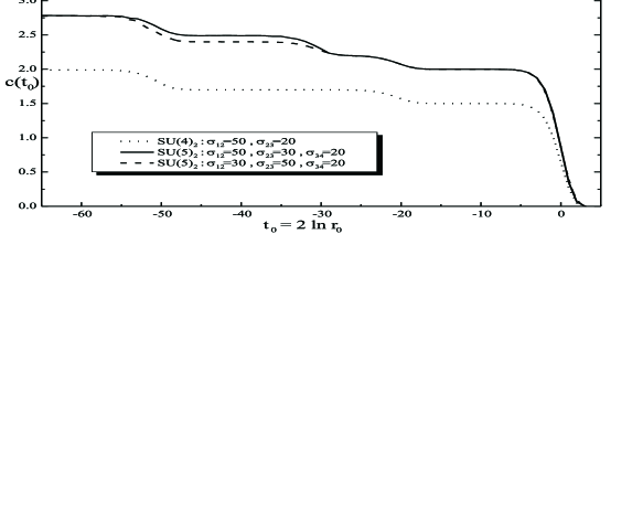
Figure 5.1: Renormalisation group flow for the ${c}$-function.

We observe that the $c$-function remains constant, at a value corresponding to the new coset, in some finite interval of $r_{0}$. In particular, we observe the non-equivalence of the flows when the relative order of magnitude amongst the different resonance parameters is changed. For $N=5$ we confirm (we omit here the $U(1)$-factors and report the corresponding central charges as superscripts on the last factor).

$\swarrow\qquad\qquad\searrow$
$\quad\quad SU(4)_{2}\otimes SU(2)_{2}^{\frac{5}{2}}\quad\quad\quad\quad\quad\qquad SU(3)_{2}\otimes SU(3)_{2}^{\frac{12}{5}}\qquad$
$\searrow\qquad\qquad\qquad\swarrow$
$SU(3)_{2}\otimes SU(2)_{2}\otimes SU(2)_{2}^{\frac{11}{5}}$
$\downarrow$
$SU(2)_{2}\otimes SU(2)_{2}\otimes SU(2)_{2}\otimes SU(2)_{2}^{2}$

The precise difference in the central charges is explained with (5.40), since the contribution $0.0924I_{i,i-1}$ only occurs for $i=2$.

To establish more clearly that the plateaux in Fig. 5.1 admit indeed an interpretation as fixed points, namely zeros of the corresponding $\beta$-function (see section 4.1.5) and extract the definite values of the corresponding Virasoro central charge we can also, following [24, 108], determine a $\beta$-type function from $c(r)$ along the lines of subsection 4.1.8. Our results for various values of N are depicted in Fig. 5.2, which allow a definite identification of the fixed points corresponding to the coset models expected from the decoupling (5.3).

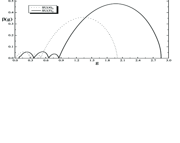
Figure 5.2: The $\beta$-function.

For $SU(4)_{2}$ we clearly identify from Fig. 5.2 the four fixed points  $\tilde{g}=0,0.3,0.5,2$ with high accuracy. The five fixed points $\tilde{g}=0,0.357,0.657,0.857,2.857$, which we expect to find for $SU(5)_{2}$ are all slightly shifted due to the absence of the higher order contributions.

5.5 Identifying the operator content of ${SU(N)_{2}}$-HSG model

In the same fashion we did for the $SU(3)_{2}$-HSG model, we now want to identify the operator content of our theory by carrying out the ultraviolet limit in the corresponding two-point functions or by using in some cases the $\Delta$-sum rule [27] and match the conformal dimension of each operator with the one in the $SU(N)_{2}/U(1)^{N-1}$-WZNW-coset model (see section 4.9). For this purpose we have to determine first of all the entire operator content of the conformal field theory.

As we did in section 4.9, we shall use the following general formula for the conformal dimensions of the parafermionic vertex operators originally derived in [59]

$$\Delta(\Lambda,\lambda)=\frac{(\Lambda\cdot(\Lambda+2\rho))}{(4+2N)}-\frac{(\lambda\cdot\lambda)}{4}\,\,.$$ (5.42)

Here $\Lambda$ is a highest dominant weight of level smaller or equal to $k=2$ and $\rho=1/2\sum_{\alpha>0}\alpha$ is the Weyl vector, i.e. half the sum of all positive roots. As explained in section 4.9 the $\lambda$’s are lower weights which are obtained from $\Lambda$ by subtracting multiples of simple roots $\alpha_{i}$ until the lowest weight is reached. Nonetheless, it may happen that a weight corresponds to more than one linear independent weight vector, such that the weight space may be more than one dimensional. The dimension of each weight vector $n_{\lambda}^{\Lambda}$ is computed by means of

$$n_{\lambda}^{\Lambda}=\frac{\sum_{\alpha>0}\sum_{l=1}^{\infty}2\,n_{\lambda+l\alpha}((\lambda+l\alpha)\cdot\alpha)}{((\Lambda+\lambda+2\rho)\cdot(\Lambda-\lambda))}\,\,\,.$$ (5.43)

For consistency it is useful to compare the sum of all these multiplicities with the dimension of the highest weight representation computed directly from the Weyl dimensionality formula (see e.g. [180])

$$\sum_{\lambda}n_{\lambda}^{\Lambda}=\dim\Lambda=\prod_{\alpha>0}\frac{((\Lambda+\rho)\cdot\alpha)}{(\rho\cdot\alpha)}\,\,.$$ (5.44)

To compute all the conformal dimensions $\Delta(\Lambda,\lambda)$ according to (5.42) in general is a tedious task and therefore we concentrate on a few distinct ones for generic $N$ and only compute the entire content for $N=4$ which we present in table 5.2.

Noting that $\,\lambda_{i}\cdot\,\lambda_{j}=K_{ij}^{-1}$, with $K$ being the Cartan matrix, we can obtain relatively concrete formulae from (5.42). For instance

$$\Delta(\lambda_{i},\lambda_{i})=\frac{4\sum_{l=1}^{N-1}K_{il}^{-1}-NK_{ii}^{-1}}{8+2N}\,\,\,.$$ (5.45)

Similarly we may compute $\Delta(\lambda_{i}+\lambda_{j},\lambda_{i}+\lambda_{j})$, etc. in terms of components of the inverse Cartan matrix. Even more explicit formulae are obtainable when we express the simple roots $\alpha_{i}$ and fundamental weights $\lambda_{i}$ of $SU(N)$ in terms of a concrete basis. For instance we may choose an orthonormal basis {$\varepsilon_{i}$} in ${\mathbb{R}}^{N}$ (see e.g. [101]), i.e. $\varepsilon_{i}\cdot\varepsilon_{j}=\delta_{ij}$

$$\alpha_{i}=\varepsilon_{i}-\varepsilon_{i+1},\,\,\,\lambda_{i}=\sum\limits_{j=1}^{i}\varepsilon_{j}-\frac{i}{N}\sum\limits_{j=1}^{N}\varepsilon_{j},\,\,i=1,\ldots N-1\,.$$ (5.46)

Noting further that the set of positive roots is given by $\{\varepsilon_{i}-\varepsilon_{j}:1\leq i<j\leq N\}$, we can evaluate (5.42), (5.43) and (5.44) explicitly. This way we obtain for instance

$$\Delta(\lambda_{i},\lambda_{i})=\frac{i(N-i)}{8+4N}\,\quad\,\text{and\quad}\,\,\Delta(2\lambda_{i},2\lambda_{i})=0.$$ (5.47)

Of special physical interest is the dimension of the perturbing operator. As was already argued in the previous chapter, it corresponds to $\Delta(\psi,0)$, with $\psi$ being the highest root and, therefore, arises for a single choice of the weights $(\Lambda,\lambda)$. Noting that for $SU(N)$ we have $\psi=\lambda_{1}+\lambda_{N-1}$, we confirm once more

$$\Delta(\psi=\lambda_{1}+\lambda_{N-1},0)=\frac{N}{N+2}\,\,,$$ (5.48)

being the expected value for the conformal dimension of the perturbing field which we will determine later for the $SU(N=4)_{2}$- and $SU(N=5)_{2}$-HSG models by studying the ultraviolet behaviour of the two-point function of the trace of the energy momentum tensor $\Theta$. Other dimensions may be computed similarly.

As mentioned before we present now the result of the computation of the entire operator content in table 5.2 for the particular coset $SU(4)/U(1)^{3}$. In case the multiplicity of a weight vector is bigger than one, we indicate this by a superscript on the conformal dimension.

$\lambda\backslash\Lambda$	$\lambda_{1}$	$\lambda_{2}$	$2\lambda_{1}$	$2\lambda_{2}$	$\lambda_{1}+\lambda_{2}$	$\lambda_{1}+\lambda_{3}$
dim $\Lambda$	$4$	$6$	$10$	$20$	$20$	$15$
$\Lambda$	$1/8$	$1/6$	$0$	$0$	$1/8$	$1/6$
$\Lambda-\alpha_{1}$	$1/8$		$1/2$		$1/8$	$1/6$
$\Lambda-\alpha_{2}$		$1/6$		$1/2$	$1/8$
$\Lambda-\alpha_{3}$						$1/6$
$\Lambda-\alpha_{1}-\alpha_{2}$	$1/8$	$1/6$	$1/2$	$1/2$	$5/8^{2}$	$1/6$
$\Lambda-\alpha_{2}-\alpha_{3}$		$1/6$		$1/2$	$1/8$	$1/6$
$\Lambda-\alpha_{1}-\alpha_{3}$						$1/6$
$\Lambda-2\alpha_{1}$			$0$
$\Lambda-2\alpha_{2}$				$0$
$\Lambda-2\alpha_{1}-2\alpha_{2}$			$0$	$0$
$\Lambda-2\alpha_{2}-2\alpha_{3}$				$0$
$\Lambda-2\alpha_{1}-\alpha_{2}$			$1/2$		$1/8$
$\Lambda-\alpha_{1}-2\alpha_{2}$				$1/2$	$1/8$
$\Lambda-2\alpha_{2}-\alpha_{3}$				$1/2$
$\Lambda-\alpha_{1}-\alpha_{2}-\alpha_{3}$	$1/8$	$1/6$	$1/2$	$1/2$	$5/8^{2}$	$2/3^{3}$
$\Lambda-2\alpha_{1}-\alpha_{2}-\alpha_{3}$			$1/2$		$1/8$	$1/6$
$\Lambda-\alpha_{1}-2\alpha_{2}-\alpha_{3}$		$1/6$		12	$5/8^{2}$	$1/6$
$\Lambda-\alpha_{1}-\alpha_{2}-2\alpha_{3}$						$1/6$
$\Lambda-2\alpha_{1}-2\alpha_{2}-\alpha_{3}$			$1/2$	$1/2$	$5/8^{2}$	$1/6$
$\Lambda-\alpha_{1}-2\alpha_{2}-2\alpha_{3}$				$1/2$	$1/8$	$1/6$
$\Lambda-2\alpha_{1}-2\alpha_{2}$					$1/8$
$\Lambda-2\alpha_{1}-2\alpha_{2}-2\alpha_{3}$			$0$	0	$1/8$	$1/6$
$\Lambda-\alpha_{1}-3\alpha_{2}-2\alpha_{3}$				$1/2$
$\Lambda-\alpha_{1}-3\alpha_{2}-\alpha_{3}$				$1/2$
$\Lambda-2\alpha_{1}-3\alpha_{2}-\alpha_{3}$				$1/2$	$1/8$
$\Lambda-2\alpha_{1}-3\alpha_{2}-2\alpha_{3}$				$1/2$	$1/8$
$\Lambda-2\alpha_{1}-4\alpha_{2}-2\alpha_{3}$				$0$

Table 5.2: Conformal dimensions for ${{\cal O}^{\Delta(\Lambda,\lambda)}}$ in the ${SU(4)_{2}/U(1)^{3}}$-WZNW coset model.

The remaining dominant weights of level smaller or equal to $2$, namely $\Lambda=\lambda_{3},2\lambda_{3},\lambda_{2}+\lambda_{3}$, including their multiplicities may be obtained from table 5.2 simply by the exchange $1\leftrightarrow 3$, which corresponds to the ${\mathbb{Z}}_{2}$-symmetry of the $SU(4)$-Dynkin diagram.

Summing up all the fields corresponding to different lower weights, we have the following operator content

$${\cal O}^{2/3},{\cal O}^{1},14\times{\cal O}^{0},8\times{\cal O}^{5/8},18\times{\cal O}^{1/6},24\times{\cal O}^{1/2},32\times{\cal O}^{1/8},$$ (5.49)

that is 98 fields. Therefore, although in section 5.3 a large number of solutions to the form factor consistency equations was found we see now that the operator content also increases quite drastically when $N$ does.

Once all the conformal dimensions of the operators of the underlying CFT corresponding to the $SU(4)_{2}$-HSG have been explicitly computed and even some of them for generic $N$ in (5.47) and (5.48) we are now in the position to obtain al least some of these dimensions by using the sum rule [27] for the operators whose symmetry makes it possible or by analysing the ultraviolet behaviour of the corresponding correlation functions computed via (4.22). Similarly to the $SU(3)_{2}$-case, whenever we find a local operator $\mathcal{O}$ for which the $\Delta$-sum rule [27] holds, we may investigate also the RG-flow of the operator content for the model at hand. We shall attempt all these tasks in the next section for the $SU(N)_{2}$-HSG models with $N=4,5$.

5.5.1 RG-flow of conformal dimensions

We will now turn to the massive model and evaluate the flow of the conformal dimension of a local operator $\mathcal{O}$ by means of Eq. (4.50), which we found in subsection 4.1.7. Recall that the field ${\cal O}$ entering Eq. (4.50) is a local operator which in the conformal limit corresponds to a primary field in the sense of [2]. In particular for $r_{0}=0$, the expression (4.50) constitutes the $\Delta$-sum rule [27] discussed in subsection 4.1.6, which expresses the difference between the ultraviolet and infrared conformal dimension of the operator ${\cal O}$.

We start by investigating the operator which in the case when all particles are of the same type corresponds to the disorder operator $\mu$ in the Ising model. Using the fact that we should always be able to reduce to that situation, we consider the solution corresponding to $\tau_{i}=\bar{\tau}_{i}=\nu_{i}=\varsigma_{i}=0$ for all $i$. Then the $\Delta$-sum rule (4.50) yields for the individual $n$-particle contributions

$$\Delta^{\mu}_{2} = (N-1)\cdot 0.0625$$ (5.50)

$$\Delta^{\mu}_{4} = (2-N)\cdot 0.0263$$ (5.51)

$$\Delta^{\mu}_{6} = (N-2)\cdot 0.0017+(3-N)\cdot 0.0113$$ (5.52)

$$\sum_{k=2}^{6}\Delta^{\mu}_{k} = 0.0266+N\ast 0.0206\,\,.$$ (5.53)

We assume that this solution has the conformal dimension $\Delta(\lambda_{1},\lambda_{1})$ in the ultraviolet limit. For comparison we report a few explicit numbers in table 5.3.

$N$	$\Delta(\lambda_{1},\lambda_{1})$	$\Delta^{\mu}_{2}$	$\Delta^{\mu}_{4}$	$\Delta^{\mu}_{6}$	$\sum_{k=2}^{6}\Delta^{\mu}_{k}$
$3$	$0.1$	$0.125$	$-0.0263$	$0.0017$	$0.1004$
$4$	$0.125$	$0.1875$	$-0.0526$	$-0.0079$	$0.1270$
$5$	$0.143$	$0.25$	$-0.0789$	$-0.0175$	$0.1536$
$6$	$0.156$	$0.3125$	$-0.1052$	$-0.0271$	$0.1802$
$7$	$0.1\bar{6}$	$0.375$	$-0.1315$	$-0.0367$	$0.2068$
$8$	$0.175$	$0.4375$	$-0.1578$	$-0.0463$	$0.2334$

Table 5.3: ${n}$-particle contributions to the $\Delta$ -sum rule versus conformal dimensions in the ${SU(N)_{2}/U(1)^{N-1}}$-WZNW coset model.

As we already observed for the $c$-theorem, the series converges slower for larger values of $N$. The reason for this behaviour is the same, namely the increasing symmetry factor. Note also that the next contribution is negative.

Following now the renormalisation group flow for the conformal dimension (4.50) by varying $r_{0}$, we assume that the $\Delta(\lambda_{1},\lambda_{1})$-field flows to the $\Delta(\lambda_{1},\lambda_{1})$-field in the corresponding new cosets. Similar as for the Virasoro central charge we may compare the exact expression

$$\Delta(\lambda_{1},\lambda_{1})_{SU(i+1)_{2}/U(1)^{i}\otimes SU(N-i)_{2}/U(1)^{N-i-1}}=$$

$$\Delta(\lambda_{1},\lambda_{1})_{SU(N)_{2}/U(1)^{N-1}}+\frac{i(N+5)(N-i-1)}{4(N+2)(i+3)(N-i+2)},$$ (5.54)

with the numerical results. The contributions (3.115)-(5.52) yield

$$\lim_{\sigma_{i,i+1}\rightarrow\infty}{\small\Delta}^{\mu}{\small(\sigma}_{i,i+1}{\small,\ldots)}$$ (5.55)

Δμ(σi,i+1=0,…)+0.0359Ii,i+1+0.0113Ij,j-1,

where again the contribution ${0.0113I}_{j,j-1}$ only occurs for $j\neq 1,N-2$. Once again we find good agreement between the two computations for small values of $N$. Our complete numerical results are presented in Fig. 5.3, which confirm the outlined flow for various values of N.

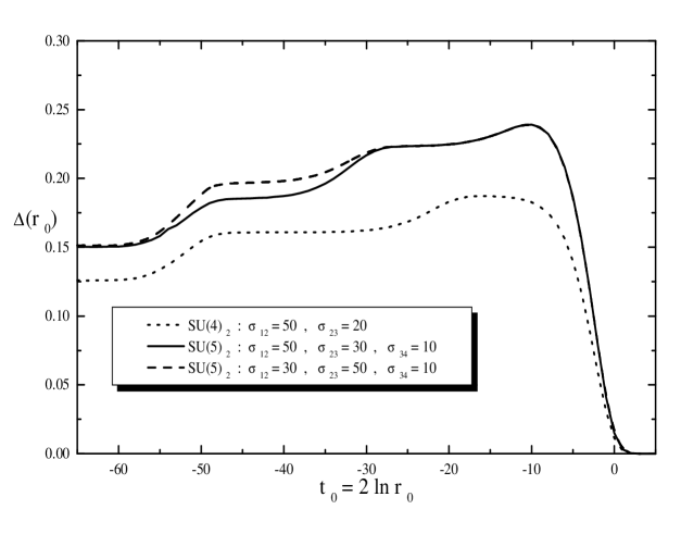
Figure 5.3: RG-flow for the conformal dimension of $\mu$.

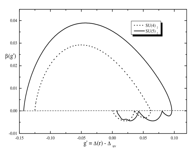
Figure 5.4: The $\beta^{\prime}$-function .

Notice by comparing Fig. 5.3 and 5.1, that, as we expect, the transition from one value for $\Delta$ to the one in the decoupled system occurs at the same energy scale $t_{0}$ at which the value of the Virasoro central charge flows to the new one which makes our picture consistent.

In analogy to (4.53) we may now define a function “$\beta^{\prime}$” and demand that it obeys the Callan-Symanzik equation [178]

$$r_{0}\frac{d}{d{r_{0}}}g^{\prime}=\beta^{\prime}(g^{\prime})\,\,.$$ (5.56)

The “coupling constant” related to $\beta^{\prime}$ is normalized in such a way that it vanishes at the ultraviolet fixed point, i.e. $g^{\prime}:=\Delta(r_{0})-\Delta_{\text{uv}}$, such that whenever we find $\beta^{\prime}(\tilde{g}^{\prime})=0$, we can identify $\hat{\Delta}=\tilde{g}^{\prime}-\Delta_{\text{uv}}$ as the conformal dimension of the operator under consideration of the corresponding conformal field theory. From our analysis of (4.50) we may determine $\beta^{\prime}$ as a function of $g^{\prime}$ by means of (5.56). Our results are presented in Fig. 5.4.

Once again, for $SU(4)_{2}$ the accuracy is very high and we clearly read off from Fig. 5.4 the expected fixed points  $\tilde{g}^{\prime}=-0.125,0,0.0375,0.0625$. The $SU(5)_{2}$-fixed points $\tilde{g}^{\prime}=-0.1429,0,0.0446,0.0821,0.1071$, are once again slightly shifted.

Notice that the behaviour of the function $\beta^{\prime}$, although it appears to be a bit peculiar is just what one expects, taking into account that the function $\Delta(r_{0})$ displayed in Fig. 5.3 is not monotonically increasing nor decreasing but it is non-decreasing in some finite interval of values of $r_{0}$ and decreases thereafter until the infrared value $\Delta_{ir}=0$ is reached. Consequently its derivative, $\beta^{\prime}$ must change sign once the energy scale for which the $\Delta(r_{0})$-function starts decreasing is reached.

5.5.2 Identifying the conformal dimension of the perturbing operator

As mentioned in several occasions, whenever the correlation function between $\mathcal{O}$ and $\Theta$ is vanishing or we consider an operator which does not flow to a primary field, we can not employ (4.50) with $r_{0}=0$ to identify the ultraviolet conformal dimension and we must resort to the well known relation reported in section 2.1 of chapter 2 and in Eq. (4.35)

$$\lim_{r\rightarrow 0}\left\langle{\cal O}(r){\cal O}(0)\right\rangle\sim r^{-4\Delta^{\!\!{\cal O}}}.$$ (5.57)

near the critical point in order to determine the conformal dimension. To achieve consistency with the proposed physical picture we would like to identify now in particular the conformal dimension of the perturbing operator which we identified in section 5.5 to be $N/N+2$. Recalling that the trace of the energy momentum tensor is proportional to the perturbing field [4] we analyse $\left\langle\hat{\Theta}(r)\hat{\Theta}(0)\right\rangle$ for this purpose and present our results in Figs. 5.5 and 5.6.

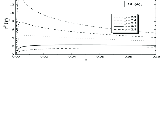
Figure 5.5: Rescaled correlation function ${G(r)=\left\langle\hat{\Theta}(r)\hat{\Theta}(0)\right\rangle}$ as a function of ${r}$ for the ${SU(4)_{2}}$-HSG model.

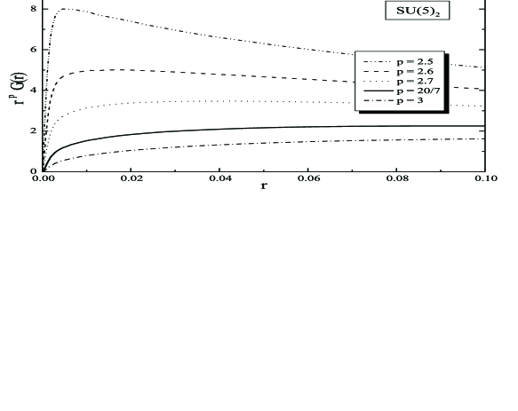
Figure 5.6: Rescaled correlation function ${G(r)=\left\langle\hat{\Theta}(r)\hat{\Theta}(0)\right\rangle\,}$ as a function of ${r}$ for the ${SU(5)_{2}}$-HSG model.

According to (5.57), we deduce from Figs. 5.5 and 5.6 that $\Delta=2/3,5/7$ for $N=4,5$, respectively, which coincides with the expected values.

5.6 Summary of results and open problems

One of the main deductions from our analysis is that the scattering matrix proposed in [51] may certainly be associated to the perturbed gauged WZNW-coset. This is based on the fact that we reproduce all the predicted features of this picture, namely the expected ultraviolet Virasoro central charge, by means of Zamolodchikov’s $c$-theorem, various conformal dimensions of local operators by means of the $\Delta$-sum rule [27] or the direct investigation of the UV-limit of the two-point correlation functions, and the characteristics of the unstable particle spectrum, that is the decoupling (5.3) which generates the sort of flows observed for the $c(r_{0})$- and $\Delta(r_{0})$-functions.

In the previous chapter we presented general $n$-particle solutions to the form factor consistency equations. Likewise, our construction of general solutions to the form factor consistency equations involves the same type of determinant building blocks found for the $SU(3)_{2}$-case. Therefore, our results support the belief that such type of determinants might constitute the basis of a generic group theoretical structure which is “hidden” in the form factor consistency equations of section 4.1. Concerning this issue, our results certainly constitute a further important step towards a generic group theoretical understanding of the $n$-particle form factor expressions. The next natural step is to extend our investigation towards higher level algebras which involves the complication outlined in the introduction.

By performing a renormalisation group analysis both of the $c$-function [24] and of the conformal dimensions [27] we found that, concerning the computation of correlation functions, our results indicate that the fast convergence of the series expansion of (4.22) observed for models involving only one stable particle, or even two, like in the $SU(3)_{2}$-case, is spoilt when the number of particles involved is large. Our concrete analysis for the $SU(N)_{2}$-HSG models seems to suggest that such a behaviour is more a consequence of the increasing importance of the symmetry factor entering the expansion (4.22) for increasing values of the particle number, than of the particular functional dependence of the corresponding form factors. Concerning the study of the convergence behaviour of (4.22), qualitative arguments providing an intuitive understanding of the suppression of the higher particle form factors in the series (4.22) have been presented in [185]. It would be interesting to generalise the latter arguments to the models under investigation and highly desirable to have more concrete quantitative criteria at hand.

Despite the fact of having identified part of the operator content, it remains a challenge to perform a definite one-to-one identification between the solutions to the form factor consistency equations and the local operators. It is clear that we require new additional technical tools to do this, since the $\Delta$-sum rule (4.50) may not be applied in all situations and (5.57) does not allow a clear cut deduction of $\Delta$ unless one has already a good guess for the expected value.

In comparison with other methods to achieve the same goal, we should note that in principle we could obtain, apart from conformal dimensions different from the one of the perturbing operator, the same qualitative picture from a TBA-analysis similar to the one performed in chapter 3. For instance, the scaling functions obtained in this chapter exhibit qualitatively the same kind of staircase pattern. However, in the TBA-approach the number of coupled non-linear integral equations to be solved increases with $N$, which means the system becomes extremely complex and cumbersome to solve even numerically. Computing the scaling function with the help of form factors only adds more terms to each $n$-particle contribution, but is technically not more involved. Therefore, again the form factor program seems to have more advantages than a TBA-analysis, the price we pay in this setting is, however, the slow convergence of (4.22).

We conjecture that the “cutting rule” (5.3) which describes the renormalisation group flow also holds for other groups different from $SU(N)$. This is supported by the general structure of the HSG-scattering matrix [51].

It would be desirable to put further constraints on the solutions to the form factor consistency equations by using the symmetries of the HSG-models, formulating quantum equations of motion, doing perturbation theory or by other means.

Chapter 6 Conclusions and open questions

Although we have already provided each of chapters 3, 4 and 5 of this thesis with a summary of the main results and open points, it is now our aim to provide the reader with a more general and concise review of all the original results presented in this thesis and also, to match the outcome of the different approaches we have exploited along the previous chapters in a way which was not possible when closing each independent chapter, since all the results had not been presented yet.

One of the main purposes of the work presented in this thesis has been the development of different non-perturbative consistency checks for the S-matrices proposed in [51] to describe the scattering theory corresponding to the Homogeneous sine-Gordon (HSG) models [49] associated to simply-laced Lie algebras. The HSG-models are particular examples of a large family of theories which are known in the literature as Non-abelian affine Toda field theories [47]. These are 1+1-dimensional theories possessing very interesting properties which have motivated their study over the last years. For instance, they are all classically integrable and, at quantum level, they give rise to two families of unitary, massive and integrable quantum field theories which have been named as symmetric space and homogeneous sine-Gordon models [48]. As we have mentioned, our work has been mainly concerned with the second class of models, although we also provided some results arising in the study of the quantum properties of the symmetric space sine-Gordon (SSSG) models.

With regard to the main objective of this work recalled above we draw the fundamental conclusion that all the results presented in this thesis confirm the consistency of the S-matrix proposal [51]. In particular, not only the concrete S-matrix proposal but also the physical picture advocated for the HSG-models in [49, 50, 51] has been confirmed by our analysis. The latter analysis has been carried out by making use of two different approaches: The thermodynamic Bethe ansatz (TBA) [20, 21] and the form factor approach [22, 153].

However, it must be emphasised that the interest of the present work is not reduced to the single (although remarkable) fact that, after different extensive tests, the S-matrices proposed in [51] have proved to be entirely consistent. An important part of our motivation has been also to contribute to the improvement of the present understanding of the thermodynamic Bethe ansatz and form factor approaches themselves. In this direction, the work presented in this thesis represents a valuable contribution, since the latter approaches had never been exploited to such an extent in the context of the study of models possessing all the novel features introduced by the HSG-models. These features are first, the parity breaking occurring both at the level of the Lagrangian and the two-particle S-matrices and second, the presence of resonance poles in the scattering amplitudes. The last characteristic is not a novel feature by itself, since other models containing resonance poles have been treated in the literature [108, 109, 110, 111, 112]. However, the novelty is that these poles admit a physical interpretation as the trace of unstable particles in the spectrum and at the same time, a well-defined Lagrangian description of the theory is available. This is not the case for many other 1+1-dimensional integrable quantum field theories (QFT’s), which are only consistent from the scattering theory viewpoint. In addition, the HSG-models are characterised by the existence of several independent mass scales, $m_{i}$, and resonance parameters, $\sigma_{ij}$, associated to resonance poles in the scattering amplitudes. This feature is also remarkable, since these models turn out to be integrable for arbitrary values of the mentioned free parameters, and the freedom for choosing their relative values gives rise to a very interesting physical picture whose interpretation is one of the most important results of the present work.

As many other 1+1-dimensional massive integrable QFT’s, the HSG-models can be understood as perturbed conformal field theories (CFT’s). The corresponding underlying CFT’s are Wess-Zumino-Novikov-Witten (WZNW) coset models [57, 58] related to cosets of the form $G_{k}/U(1)^{\ell}$, for $\ell$ to be the rank of the Lie algebra $g$ associated to the Lie group $G$ and $k$ to be an integer called the level. Such CFT’s are also known under the name of $G_{k}$-parafermion theories [59, 60, 61]. It is worth mentioning that even the simplest examples of HSG-models associated to the lowest values of the rank of the Lie algebra, $\ell$, and the level, $k$, give rise to theories whose operator content is quite involved. This is related to the fact that the underlying CFT’s corresponding to the HSG-models have always Virasoro central charge $c>1$, which implies the existence of infinitely many conformal primary fields in the unperturbed theory. This aspect is responsible of some of the most interesting results obtained within the form factor framework: the understanding of the momentum space cluster property not as a mere property observed for the form factors of some particular theories but also as a construction principle of solutions to the form factor consistency equations [22, 153, 152, 154, 155], and the re-construction of a large part of the operator content of a quantum field theory by exploiting the knowledge of the operator content of its underlying CFT and of the correlation functions involving the mentioned operators, available in the form factor context.

Recall that, the thermodynamic Bethe ansatz and form factor approach are non-perturbative methods which allow, amongst other applications, for reproducing the most characteristic data of the underlying CFT arising in the UV-limit of a certain 1+1-dimensional QFT. The starting point for carrying out both, a TBA- or a form factor analysis, is the knowledge of the exact S-matrix characterising the latter QFT and consequently its mass spectrum. Provided this initial input, which is available for many 1+1-dimensional integrable massive QFT’s due to their distinguished properties, the following quantities characterising the unperturbed CFT and massive QFT are in principle extractable:

i) the Virasoro central charge of the underlying CFT,

ii) the flow of the Virasoro central charge of the ultraviolet CFT from its critical value to the infrared limit, surpassing the different energy scales fixed by the coupling constants of the model. It is possible to construct different functions reproducing qualitatively the same type of flow namely, carrying the same physical information. In the TBA- and form factor approach these functions are the so-called finite size scaling function [23] and Zamolodchikov’s c-function [24], respectively. Both functions admit an interpretation as a measure of effective light degrees of freedom in a QFT. They reproduce the successive decoupling of massive degrees of freedom of the QFT as soon as the energy necessary for the onset of a certain particle in the spectrum is much higher that the temperature of the system or energy scale considered,

iii) the conformal dimension of the perturbing field which takes the underlying CFT away from its renormalisation group fixed point in the construction of the massive QFT [18],

iv) the conformal dimensions of other local operators arising in the underlying CFT different from the perturbing field. In other words, one may be able to reconstruct, at least partially, the operator content of the underlying CFT (at least for the primary fields) by exploiting data characteristic from the massive QFT and assuming a one-to-one correspondence between the operator content of the unperturbed CFT and the massive QFT,

v) the renormalisation group flow of the operator content of the underlying CFT from the ultraviolet to the infrared limit by explicit evaluation of the conformal dimensions of certain local operators of the unperturbed CFT as functions of the renormalisation group parameter,

vi) the correlation functions involving certain local operators of the massive QFT, whose UV-behaviour is governed by the ultraviolet conformal dimension of the operator under consideration.

We will now report in more detail our original results, going through each of the previous points and explaining how these quantities may be available within each of the approaches considered. As stressed along the different chapters, the results presented in this thesis may be found in [56, 68, 72, 73, 28, 74]:

Concerning the evaluation of the Virasoro central charge of the underlying CFT in the TBA-framework, in the deep ultraviolet limit we recover the $G_{k}/U(1)^{\ell}$-coset central charge for any value of the $2\ell-1$ free parameters entering the S-matrix, including the choice when the resonance parameters vanish and parity invariance is restored on the level of the TBA-equations. This is in contrast to the properties of the S-matrix, which is still not parity invariant due to the occurrence of the phase factors $\eta$, which are required to close the bootstrap equations [51]. The same observations hold in the form factor context. However, within the latter framework, the Virasoro central charge of the underlying CFT has been explicitly evaluated only for some concrete models by means of Zamolodchikov’s $c$-theorem [24]. Therefore, in what concerns the evaluation of the UV central charge of the underlying CFT, both the concrete models studied and the nature of the results obtained are quite different in the TBA- and form factor analysis.

Whereas in the TBA-context the Virasoro central charge can be exactly determined due to the fact that the TBA-equations admit an analytical solution in the deep UV-limit for any HSG-model, in the form factor context the central charge can be evaluated numerically with a certain accuracy which is very high when the rank of the Lie algebra is small but becomes worse as soon as the rank is increased. Recall that the number of stable particles in the model is given by $\ell\times(k-1)$ which means increasing (decreasing) the rank of the Lie algebra is equivalent to increasing (decreasing) the number of particles in the spectrum. Moreover, the evaluation of the Virasoro central charge is the form factor context has been carried out only for some of the $SU(N)_{2}$-HSG models, which is in contrast with the generality of the results available in the TBA-context. Technically, the computation of the Virasoro central charge by means of Zamolodchikov’s $c$-theorem [24] requires the numerical computation of a series of multi-dimensional integrals arising in the expansion of the two-point function of the trace of the energy momentum tensor in terms of its associated $n$-particle form factors. Since the mentioned series contains in general an infinite number of terms and it is not known for the time being how to sum exactly all these terms, one has to evaluate separately each individual contribution to the expansion. Furthermore, the dimension of the integrals increases with the number of particles and with the order of the term in the series, which means for a reasonable computer time, the numerical methods available at present only permit to evaluate the first contributions to the expansion. Our particular analysis has shown that for the $SU(3)_{2}$-HSG model the value of the Virasoro central charge can be obtained with high accuracy by summing terms up to the 6-particle contribution. This is still true for the $SU(4)_{2}$- and $SU(5)_{2}$-HSG models but for higher values of the rank of the Lie algebra the precision reached gets worse and one might be forced to take into account contributions from higher order terms.

As we have mentioned, the same value for the central charge is obtained for every finite value of the resonance parameters, which reflects the fact that in the ultraviolet limit parity invariance is restored both at the level of the TBA-equations and also when evaluating the central charge by means of Zamolodchikov’s $c$-theorem in the form factor context. The underlying physical behaviour is, however, quite different for different values of the resonance parameters as our numerical analysis has demonstrated. The numerics turn out to be entirely consistent with the physical picture anticipated in [49, 50, 51] for the HSG-models in the two approaches we have analysed. In the TBA-framework we have evaluated numerically the finite size scaling function [23] whereas its counterpart when using form factors has been Zamolodchikov’s $c$-function [24]. Both functions turned out to have an entirely analogous qualitative behaviour. They exhibit a very characteristic “staircase” pattern in their flow from the UV- to the IR-regime similar to the one found in [108] for the roaming trajectory models. However, in the latter case the scaling function is characterised by infinitely many plateaux, whereas for the HSG-models only a finite number of plateaux, in correspondence to the amount of free parameters available in the quantum theory, was found. Also, for the HSG-models, the interpretation of the scaling functions as a measure of light degrees of freedom in the QFT allows for a clear physical interpretation of the results obtained:

• For vanishing resonance parameter $\sigma=0$ and taking the energy scale of the stable particles to be of the same order $m_{1}\simeq m_{2}$, the deep ultraviolet coset central charge is reached straight away. From the physical point of view this is the expected behaviour since, according to Breit-Wigner formula (2.102), (2.103), whenever the resonance parameter is vanishing, the same happens to the decay width of the unstable particles. Therefore, the unstable particles become ‘virtual states’ associated to poles on the imaginary axis beyond the physical $\theta$-sheet and they are on an energy scale of the same order as the one of the stable particles. Being the energy scale corresponding to the onset of all stable and unstable particles of the same order the scaling function takes the value corresponding to the ultraviolet coset central charge of the underlying CFT as soon as the mentioned scale is reached.

• On the other hand, for non-vanishing resonance parameter the scaling function and Zamolodchikov’s $c$-function surpass different regions in the energy scale developing a “staircase” behaviour where the number and size of the plateaux is determined by the relative mass scales between the stable and unstable particles and the stable particles themselves. Therefore, different choices of the $2\ell-1$ free parameters at hand lead to a theory with a different physical content, but still possessing the same central charge. This feature is consistent with the physical picture anticipated for the HSG-models, since in the deep ultraviolet limit, as long as the resonance parameter is finite, the energy scale is much higher than the energy scales necessary for the production of all the stable and unstable particles. Therefore all the particle content of the model contributes to the scaling function which, interpreted as a measure of effective light degrees of freedom, will reach its maximum value, namely the Virasoro central charge of the unperturbed CFT.

The concrete models for which the scaling function and the $c$-function have been evaluated are different. Whereas in the TBA-context we focused our study in the $SU(3)_{k}$-HSG models and evaluate the scaling function for $k=2,3$ and $4$, in the context of form factors, we studied the opposite case namely, we fixed the level $k=2$ and tuned the rank of the Lie algebra. This shows that the two approaches exploited here are somehow complementary, since the solution of the TBA-equations, even numerically, gets very involved when the rank increases whereas in the form factor context the increment of the level means the existence of asymptotic bound states in the theory which make the so-called bound state residue equations enter the analysis, complicating the evaluation of the corresponding form factors. In particular the $SU(3)_{2}$-HSG model is the only one which has been studied in both approaches, being the results obtained entirely consistent.

Concerning the computation of the scaling function and the $c$-function, the evaluation of the latter in the form factor context provides very interesting results when the rank is increased which have not a counterpart in our TBA-analysis. In particular the decoupling of the $SU(N)_{2}$-HSG model into the $SU(i+1)_{2}$- and $SU(N-i)_{2}$-HSG models whenever the resonance parameter $\sigma_{i,i+1}\rightarrow\infty$, provides a further consistency check for the corresponding S-matrices. Although, as we have said, such a decoupling has not been studied in the TBA-context apart from the $N=3$ case, what has been exploited in the latter approach is the freedom for considering the mass scales of the stable particles to be very different, which generates an additional plateau in the scaling function for the $SU(3)_{k}$-HSG models. In the form factor context the mass scales of the stable particles have been always taken to be of the same order and only the freedom for varying the masses of the unstable particles which depend on the resonance parameters has been used in order to reproduce the outlined decoupling.

Another interesting result concerning the evaluation of the scaling and $c$-function is that the sort of flows described by the first of these functions are associated to a system of TBA-equations which, after the introduction of the auxiliary parameter $r^{\prime}=r/2e^{\sigma/2}$, can be re-interpreted as the TBA-equations corresponding to two massless systems, in the spirit of [126]. However, the connection between flows related to the presence of unstable particles in the spectrum and massless flows was observed only formally in the TBA-context, since the parameter $r^{\prime}$ was introduced aiming towards a simplification of the analytical and numerical analysis. Our later renormalisation group analysis has confirmed that the parameter $r^{\prime}$ has in fact a deeper physical meaning and arises naturally when studying different sorts of renormalisation group flows, supporting the idea that the observed flows should be in fact understood as massless flows.

The similar “staircase” behaviour observed both for the HSG-models and for the models studied in [108, 109, 110] has been emphasised many times along this thesis. However, the features and interpretation of this staircase pattern are very different for the models studied in [108, 109, 110] and for the ones investigated in this thesis. First of all, although both for the former and the latter models resonance poles are present in the scattering amplitudes, only for the HSG-models these poles admit a physical interpretation as the trace of the presence of unstable particles which is supported by all the results found in this manuscript. Second, and closely related to the first observation, the amount of plateaux present in the scaling functions of the HSG-models is intimately related to the amount of particles, both stable and unstable, in the spectrum. Consequently, the number of plateaux observed is always finite, which is in contrast to the roaming trajectory models [108] and their generalisations [109, 110], whose scaling functions were shown to develop infinitely many plateaux.

Whereas for the HSG-models the resonance parameter enters the S-matrix as a shift in the rapidity variable, in the models studied in [108, 109, 110] the resonance parameter arises as a consequence of the analytical continuation to the complex plane of the effective coupling constant $B$, which characterises the Lagrangian and S-matrix of the sinh-Gordon model [43] and, in fact, of all affine Toda field theories [35, 36, 39]. The mentioned complexification takes place in the following way

$$B\rightarrow 1\pm\frac{2i\sigma}{\pi}.$$ (6.1)

It is interesting to notice that the particular form of (6.1) has an explanation. The real part of $B$ has necessarily to be one so that the consequent transformation of the sinh-Gordon S-matrix via (6.1) generates a new but still consistent S-matrix. The consistency of the new S-matrix in guaranteed by the fact that for all affine Toda field theories [35, 36, 37] the coupling constant $B$ occurs always in the combination $B(2-B)$ which stays real under (6.1).

The introduction of the resonance parameter $\sigma$ by means of (6.1) makes the S-matrix exhibit a resonance pole in the imaginary axis $\theta_{R}=-\sigma-\frac{i\pi}{2}$ similarly to the $SU(3)_{2}$-HSG model. As usual one could try to understand such pole as the trace of an unstable particle. However, even though only one resonance parameter has been introduced, the TBA-analysis carried out in [108] for the roaming sinh-Gordon model shows that the corresponding scaling function develops an infinite number of plateaux. Therefore, the results in [108] can not be interpreted physically by using the same sort of arguments employed in the TBA-analysis of the HSG-models. Equivalently, the infinite number of plateaux observed in [108] can not be related to the number of free parameters in the model. The same can be said with respect to the models studied in [109, 110] whose construction follows the same lines summarised for the roaming sinh-Gordon model, with the difference that they take as an input the S-matrices of other simply laced affine Toda field theories instead of the sinh-Gordon model ($A_{1}^{(1)}$-ATFT), which is the simplest of their class.

An interesting open problem is the investigation of the precise relationship between the scaling function arising in the TBA-context and Zamolodchikov’s $c$-function. As we have repeatedly mentioned, both functions provide the same physical information and are qualitatively very similar. However, by reviewing their definitions and the contexts in which they arise, we find that the nature of their possible relationship is not clear a priori. Also the relation to the intriguing proposal in [182] of a renormalisation group flow between Virasoro characters remains unclarified.

Regarding now point iii), the evaluation of the conformal dimension of the perturbing operator, $\Delta$, has been performed both in the TBA- and form factor approach. Both methods have supplied entirely consistent results.

In the TBA-context, the computation of the conformal dimension of the perturbing field is possible by exploiting its relation to the periodicities of the so-called $Y$-systems, noticed originally in [139], despite the fact that the reason why this relationship should occur is not known for the time being. The mentioned conformal dimension also arises in the series expansion of the finite size scaling function in terms of the inverse temperature of the system. In this thesis we have exploited the former relationship and identified the conformal dimension of the perturbing field by determining the periodicities of the $Y$-systems corresponding to various concrete examples of $SU(3)_{k}$-HSG models corresponding to $k=2,3,4$. However, we have not been able to provide a general formula expressing the dependence between these periodicities and the conformal dimension of the perturbation. Such a relationship has been conjectured in the light of the particular results obtained for concrete models and more work is needed in order to make a definite statement. Nevertheless, for vanishing resonance parameter and the choice $g=su(2)$, the behaviour observed coincides with the one obtained in [139], which suggests the conjectured dependence of the periodicities of the $Y$-systems in $\Delta$ is of a very universal nature, beyond the models discussed here. In order to clearly determine the conformal dimension of the perturbation it would be very interesting to carry out the mentioned series expansion of the scaling function in terms of the inverse temperature, $r$.

Within the form factor framework, the identification of the conformal dimension of the perturbing operator has been done for the particular $SU(N)_{2}$-HSG models, with $N=3,4,5$. In that case three fundamental results have been exploited: first of all, the proportionality between the perturbing field and the trace of the energy momentum tensor of the massive QFT is well known [163]. Second, once the form factors of the trace of the energy momentum tensor are known its two-point function may be computed up to a certain approximation, as explained for the Virasoro central charge. Third, in the UV-limit the two-point function of the trace of the energy momentum tensor must reduce to the two-point function of its counterpart in the underlying CFT. That is a quasi-primary field of the CFT whose two-point function is forced to diverge in the UV-limit as $r^{-4\Delta}$ in terms of the conformal dimension of the perturbation.

Since the perturbing operator plays a distinguished role in the construction of the massive QFT, the identification of its conformal dimension constitutes a fundamental check for the consistency of the proposed S-matrices. However, once the perturbing field has been identified, one may pose the question of how to identify the remaining operator content of the underlying CFT. With regard to point iv), the re-construction of the operator content of the unperturbed CFT from the one of the massive QFT, apart from providing a further consistency check of the S-matrices under consideration, is an issue which has great interest in its own right. Fortunately, the operator content is well known for the WZNW-coset theories [59, 61], a fact of which our investigation has taken advantage. Another relevant aspect is that it becomes soon fairly involved even for low rank Lie algebras. The latter feature was an additional motivation for our analysis, since to our knowledge, no other QFT’s possessing such an involved operator content had been studied before to such an extent in the form factor context, at least for the purpose outlined.

Nonetheless, the question of how to identify the whole operator content of the underlying CFT is left unanswered in the TBA-framework. In fact, one of the most important results of this thesis has been the identification of the form factor approach as a means for re-constructing at least an important part of the operator content of the unperturbed CFT. Such a re-construction makes use of the fundamental assumptions of the existence of a one-to-one correspondence between the operator content of the massive QFT and its associated underlying CFT and between the solutions to the form factor consistency equations and the local operators of the massive QFT. The mentioned identification of part of the operator content has been performed to a large extent for the $SU(3)_{2}$-HSG model and for one of the local operators of the $SU(N)_{2}$-HSG models. For all the $SU(N)_{2}$-HSG models, a large subset of solutions to the form factor consistency equations have been constructed which permitted the former investigation.

As we have said in the previous paragraph, the identification of an important part of the operator content of the massive QFT within the form factor approach has been mainly performed for the $SU(3)_{2}$-HSG model via the calculation of the corresponding ultraviolet conformal dimension of those operators for which all the $n$-particle form factors had been previously computed. In particular, the conformal dimension of the perturbing operator ($\Delta=3/5$) and of several other operators of conformal dimension $\Delta=1/10$ were obtained by studying the ultraviolet behaviour of their two-point functions, which is constrained by the conformal symmetry of the underlying CFT. For some operators we have determined the conformal dimensions by means of the $\Delta$-sum rule derived in [27], which involves the knowledge of the correlation functions of a certain local operator and the trace of the energy momentum tensor and whose derivation is close in spirit to Zamolodchikov’s $c$-theorem.

In this light, it can be stated that solutions of the form factor consistency equations can be identified with operators in the underlying CFT. In this sense one can give meaning to the operator content of the integrable massive model. Being the mentioned identification uniquely based on the values of the ultraviolet conformal dimensions there is the problem that once the conformal field theory is degenerate in this quantity, as it is the case for the models we investigate, the identification can not be carried out in a one-to-one fashion and therefore the procedure has to be refined. In principle this would be possible by including the knowledge of the three-point coupling of the conformal field theory and the vacuum expectation value into the analysis. The former quantities are in principle accessible by working out explicitly the conformal fusion structure, whereas the computation of the latter still remains an open challenge. In fact, what one would like to achieve ultimately is the identification of the conformal fusion structure within the massive models. Considering the total number of operators present in the conformal field theory (a $SU(3)_{2}/U(1)^{2}$-WZNW coset theory for the $SU(3)_{2}$-HSG model ) one still expects to find additional solutions, in particular the identification of the fields possessing conformal dimension $\Delta=1/2$ is outstanding.

Despite the fact of having identified some part of the operator content, it remains a challenge to perform a definite one-to-one identification between the solutions to the form factor consistency equations and the local operators, at least for the primary field part. In this direction our analysis also proves that new additional technical tools are required to do this, since the $\Delta$-sum rule can not be applied in all situations, and the study of the ultraviolet behaviour of the two-point functions does not allow a clear-cut deduction of $\Delta$ unless one has already a priori a good guess for the expected value.

With respect to the explicit calculation of conformal dimensions, technically we have confirmed that the mentioned sum rule is clearly superior to the direct analysis of the UV-limit of correlation functions. However, it has also the drawback that the existence of internal symmetries in the massive QFT may force the two-point function of a large number of local operators with the trace of the energy momentum tensor to vanish and so, it only applies for part of the operator content. It would therefore be highly desirable to develop arguments which also apply for theories with internal symmetries and possibly to resolve the mentioned degeneracies in the conformal dimensions.

Concerning point v), we have also exploited the mentioned $\Delta$-sum rule as as a tool which allows for determining the flow of the operator content of a certain CFT from the UV- to the IR-limit, in a similar spirit to the scaling and $c$-function described above. For this purpose, we have modified the original sum rule derived in [27] by the introduction of the renormalisation group parameter, $r_{0}$, whose variation from the deep UV-limit, in which we expect to recover the conformal dimension of an operator of the underlying CFT, to the IR-regime reveals the same physical picture observed when studying the RG-flow of Zamolodchikov’s $c$-function. Accordingly, the corresponding $\Delta(r_{0})$-function develops a series of plateaux whose form and size depend upon the relative mass scales of the stable and unstable particles. This function has been numerically determined for the $SU(N)_{2}$-HSG models corresponding to $N=3,4,5$ and for different values of the resonance parameters, reproducing again the decoupling of massive degrees of freedom whenever one of the resonance parameters is very large in comparison to the scale fixed by the RG-parameter $r_{0}$.

As mentioned above, the physical information extractable from the scaling function, Zamolodchikov’s $c$-function and the $\Delta(r_{0})$-function associated to a certain operator of the massive QFT is mostly the same. In particular, all these functions develop plateaux which are commonly identified with RG-fixed points. In order to have a more clear-cut identification of these fixed points it is desirable to have new functions at hand whose zeros are precisely in one-to-one correspondence with the plateaux mentioned before. If we now think of Zamolodchikov’s $c$-function, the sort of functions we are looking for have similar features to the $\beta$-functions entering the Callan-Symmanzik equation [178], which are always vanishing at RG-fixed points. However, any function proportional to the derivative of the scaling function, Zamolodchikov’s $c$-function or the $\Delta(r_{0})$-functions may have also zeros where the latter functions had plateaux. In this thesis we have exploited this simple observation in order to construct what we called $\beta$-like functions, originally introduced in [108]. This has been performed for the $SU(4)_{2}$- and $SU(5)_{2}$-HSG models and allowed for clearly identifying the different RG-fixed points the three mentioned functions surpass along their respective flows.

Concerning point vi), we have already mentioned many times the possibility of computing correlation functions from form factors. In principle, any correlation function involving local operators of the massive QFT can be computed provided all $n$-particle form factors associated to these local operators are known. In practise, we have seen that the correlation functions admit a series expansion in terms of form factors of the operators involved, whose exact evaluation is outstanding for all models except for the thermally perturbed Ising model. In the thermally perturbed Ising model the two point functions $\langle\Theta(r)\Theta(0)\rangle$, $\langle\Theta(r)\mu(0)\rangle$, $\langle\Theta(r)\Sigma(0)\rangle$, involving the trace of the energy momentum tensor and the order and disorder operators can be exactly evaluated, since the only non-vanishing form factor of the trace of the energy momentum tensor is the two-particle one, and the corresponding integrals can even be performed analytically. However, this is not the case for the models we have studied here and in our analysis we have summed at most terms up to the 8-particle contribution, which already requires a lot of computational effort. Also, although we already pointed it out in the context of the evaluation of the Virasoro central charge, we have observed in this thesis that the common assumption that the mentioned series converges rapidly does not hold anymore when the number of particle types present in the model increases.

Regarding the form factor program itself, our main results are the following. At the mathematical level, a closed formula for all $n$-particle form factors associated to a large class of operators has been found for all $SU(N)_{2}$-HSG models. This formula is given in terms of building blocks which can be expressed both as determinants whose entries are elementary symmetric polynomials or by means of an integral representation. However, it remains an open question, whether the general solution procedure presented in chapters 4 and 5 can be generalised to the degree that determinants of the type found will serve as generic building blocks of form factors. It remains also for us to be understood how the integral representation obtained for these determinants might be used in practise, for instance, to formulate rigorous proofs of the type presented in the previous two chapters. In general, it would be very interesting to clarify whether such a representation has a purely formal nature or it is maybe more fundamental than the determinant representation we have exploited in this thesis. Another interesting open problem is to find out the precise relationship between this integral representation, which involves contour integrals in the $x=e^{\theta}$-plane, and the integral representation used for instance in [155] which involved contour integrals in the $\theta$-plane.

It would be also desirable to put further constraints on the solutions to the form factor consistency equations in order to make more clear their identification with a particular local operator of the model. As we have mentioned, such an identification has being carried out by analysing the UV-behaviour of the corresponding two-point functions, a procedure which has the inconveniences already reported. The identification procedure could be possibly refined by means of other arguments, that is, exploiting the symmetries of the model, formulating quantum equations of motion, possibly performing perturbation theory etc…

Concerning the momentum space cluster property, our analysis also provides remarkable results. We have shown for a concrete model, the $SU(3)_{2}$-HSG model, that it does not only constrain the solutions to the form factor consistency equations but also serves as a construction principle for new solutions. Clearly, it would be very interesting to develop arguments which allowed us to reach a level of understanding of this property similar to the one we have for the rest of the form factor consistency equations [22, 153, 152, 154, 155].

As a way to close this chapter, we can draw the overall conclusion that the physical picture advocated for the $SU(N)_{2}$-homogeneous sine-Gordon models in [49, 50, 51], rests now on quite firm ground and, apart from the open problems already mentioned along this chapter, there is also the more general challenge to extend our analysis to the complete generality of the HSG-models. Also, although it has only been mentioned very briefly in chapter 2 of this thesis, there is still a lot of interesting work to be done in what concerns the study of the other family of unitary, massive and quantum integrable NAAT-theories, the symmetric space sine-Gordon models [48, 56, 55], which is left for future investigations.

Acknowledgments

Before I add here, in my mother tongue, the original acknowledgments which appear in the version of this thesis, presented on the 31st July 2001, I would like in addition to express my acknowledgment to my thesis supervisor J.L. Miramontes Antas for introducing me to this field of research, and to the members of my thesis commission, P.E. Dorey, A. Fring, G. Mussardo, J. Sánchez Guillén and G. Sierra Rodero, for their participation and judgment. I am very specially indebt to A. Fring, in collaboration with who a large part of this work was carried out, and to P. Dorey and G. Mussardo, for sending me various valuable comments and suggestions.

This work has been supported partially by DGICYT (PB96-0960), CICYT (AEN99-0589), the EC Commission via a TMR Grant (FMRX-CT96-0012), Institut für Theoretische Physik, Freie Universität Berlin and Deutsche Forschungsgemeinschaft (Sfb288).

Berlin, 4 de xuño do 2001

Queridos colegas e amigos,

Penso que a presentación da miña tese doutoral é acontecemento de suficiente importancia como para, alomenos intentar, facer xustiza a todos aqueles que sodes, dun xeito ou doutro, responsables de que as páxinas que seguen estean agora nos vosas mans. Agardo que saibades perdoa-la lonxitude do que segue (no que a agradecementos se refire) mais, tiven a fortuna neste tempo de contar co apoio persoal e/ou profesional de moitas persoas, e non quixera, nunha ocasión coma esta, esquecer a ninguén.

Adicarei pois a miña primeira mención ó Catedrático desta universidade, D. José Luis Miramontes Antas. Gracias a él tiven a oportunidade de traballar en Física Teórica, un traballo non sempre doado, pero que me proporcionou, e ainda o fai, moitas satisfaccións.

A Luis Miramontes débolle tamén a miña introducción ó campo máis específico dos sistemas integrables en 1+1-dimensións, compartindo comigo a súa ampla experiencia no que se refire ás teorías de Toda non abelianas, tan presentes, tanto no meu traballo de tesiña, coma na tese que vai a continuación.

Dada a enorme relevancia que a colaboración coa Freie Universität Berlin, en particular con Andreas Fring, tivo para a realización desta tese, quixera tamén agradecerlle a Luis Miramontes o seu apoio ás miñas diferentes estancias en Berlín durante o ano 2000, impartindo incluso parte das horas de docencia que a min me correspondían, e a súa interese no traballo desenvolvido nestes períodos.

Finalmente, non podo deixar de agradecerlle a Luis Miramontes a lectura exhaustiva deste manuscrito a cal, de seguro, ten contribuido á mellora na presentación dos resultados obtidos, e as moitas discusións mutuas e tempo adicado a miña formación nestes anos de doutorado.

En segundo lugar, aínda que, definitivamente, non menos importante para a realización desta tese, debo menciona-la colaboración con Andreas Fring, da Freie Universität Berlin.

Penso que non será necesario poñer demasiada énfase na importancia de dita colaboración, a cal queda clara á luz da lista de artigos nos que esta tese se basea, e que presento algunhas follas más adiante.

De seguro, todo o que aquí poida dicir será insuficiente, no que respecta ó meu agradecemento a Andreas Fring, mais farei o posible por mencionar, alomenos, os aspectos máis relevantes:

Profesionalmente, debo agradecerlle o ter compartido connosco a súa ampla experiencia na amplicación do denominado ‘Bethe ansatz termodinámico’ a diferentes teorías integrables en 1+1-dimensións, o cal deu lugar ó primeiro froito da nosa colaboración. Para él vai tamén o meu agradecemento por terme introducido ó campo do cálculo de factores de forma e ás diferentes aplicacións de tales obxectos. Agradézolle tamén o ter compartido comigo a súa experiencia no referente ós diferentes métodos computacionais que son imprescindibles, tanto no campo de factores de forma, coma no contexto do Bethe ansatz termodinámico.

De xeito máis xeral, debo agradecerlle a Andreas Fring a enorme confianza que depositou en min dende a miña primeira visita a Berlín, facendo posibles outras dúas visitas posteriores, parcialmente financiadas pola Freie Universität Berlin, e propoñéndome e apoiándome posteriormente para o posto que ocupo na actualidade. Tanto durante as mencionadas estancias en Berlín, coma durante a súa estancia na Universidade de Santiago de Compostela, en novembro do 2000, coma na actualidade, débolle incontables descusións e explicacións e agradézolle, dun xeito moi especial, o seu constante aprecio e respeto pola miña contribución ó noso traballo en común, que de seguro aumentou a miña motivación e seguridade. Tamén debo extende-lo meu agradecemento a un plano máis persoal, xa que tiven (e teño) a fortuna de contar con apoio persoal e amistade de Andreas Fring, aspectos que foron de gran importancia no desenvolvemento do noso traballo en común, facéndoo máis levadeiro e fructífero. Este apoio foi especialmente importante durante a etapa de escritura desta tese doutoral, e tamén na miña adaptación (aínda en progreso) a unha nova vida en Berlín.

Para rematar, quero agradecerlle a Andreas Fring a súa lectura coidadosa desta tese, que a mellorou sustancialmente e tamén o terme dado a oportunidade de traballar cunha persoa á que só poido calificar como humana e profesionalmente excepcional.

Continuando estes longos agradecementos, non podo esquecer a Christian Korff, persoa coa que tamén tiven a sorte de colaborar, en dúas das publicacións que se recollen nesta tese. Agradézolle de xeito especial a súa amabilidade e enorme axuda durante a miña primeria estancia en Berlín, en marzo do 2000, e o seu talante persoal, que fixo sempre agradables e levadeiras as horas de traballo en común.

A continuación, quero adicar tamén unha especial mención ó Catedrático da Universidade de Santiago, D. Joaquín Sánchez Guillén, pola súa continua interese, tanto no meu traballo de tesiña coma nesta tese doutoral e adicionalmente, por ter sido a súa visita a Berlín, no verán do ano 1999, a que fixo posible a posterior estancia de Christian Korff no Departamento de Física de Partículas da Universidade de Santiago e, polo tanto, propiciou o comenzo da colaboración xa mencionada con anterioridade.

Quixera tamén agradecerlle ó Profesor da Freie Universität Berlin, Robert Schrader, o ter autorizado a financiación de parte das miñas estancias en Berlín no ano 2000 e tamén a súa acollida no grupo que encabeza, tanto naqueles períodos, coma na actualidade.

Non podo deixar de mencionar aquí ó Profesor Emérito da Freie Universität Berlin, Bert Schroer, pola gran interese que mostrou no traballo desenvolvido nesta tese e os interesantes comentarios e suxerencias que, referentes ó seu contido, nos fixo chegar nos últimos meses.

De xeito xeral quero expresárlle-lo meu agradecemento a tóda-los membros do Departamento de Física de Partículas da Universidade de Santiago, polo inmellorable ambiente de traballo e compañeirismo no que tiven a oportunidade de iniciar a miña formación. Tamén, quero adicárlle-lo meu agradecemento, a tódo-los membros do grupo encabezado polo profesor Robert Schrader do Institut für Theoretische Physik, Freie Universität Berlin, pola súa amabilidade e boa acollida, tanto durante as miñas diferentes estancias do ano pasado, coma dende a miña incorporación como membro do mencionado grupo, en febreiro deste ano.

Ademais das anteriores persoas, debo mencionar tamén a outras moitas, a axuda das cales está máis ligada o plano da amistade ca ó científico mais que, non obstante, foron tamén moi importantes para o desenvolvemento do traballo que se presenta aquí e encheron de lembranzas agradables os meus anos de doutorado.

En primeiro lugar, pola súa axuda impagable durante o período de escritura desta tese, teño que citar a Ricardo Vázquez, unha persoa á que me une unha gran amistade persoal. Penso que non tería sido capaz de escribir esta tese no tempo no que o fixen se non tivese contado coas súas moitas palabras de ánimo e a súa confianza na miña capacidade para facelo. Neste senso, a súa axuda e constante apoio persoal foron, e son aínda agora, moi importantes. Agradézolle tamén a súa interese no meu traballo, e a súa axuda no desenvolvemento dalgunhas das partes desta tese, ó compartir comigo a súa experiencia na programación en FORTRAN, facendo así posible unha parte importante dos cálculos numéricos que levei a cabo.

En segundo lugar, quero tamén mencionar a dúas persoas ás que tamén me une a amistade persoal: Dolores Sousa e Jaime Álvarez, ambos compañeiros do departamento de Física de Partículas da Universidade de Santiago. Gracias a eles, e en xeral, a tódo-los meus compañeiros do despacho 009: Félix del Moral, Carlos Lozano e, a xa mencionada, Dolores Sousa, puiden traballar nunha atmosfera inmellorable de compañeirismo. Con Dolores Sousa compartín incontables conversacións, cafés matutinos e horas de traballo. A súa vitalidade e carácter optimista foron fundamentais para min en moitas ocasións, así coma os seus intelixentes consellos e continuo apoio persoal no tempo no que compartimos despacho. A Jaime Álvarez, compañeiro do despacho 003, agradézolle tamén un montón de conversacións que me axudaron en momentos difíciles, o ter sempre palabras de ánimo e amistade para min, e formar parte de moitas das miñas lembrazas máis positivas da etapa de tese.

Ademais, debo mencionar tamén ós veciños do despacho 005, Máximo Ave, Jose Camino, Marta Gómez-Reino e César Seijas con quen compartín tamén moito do meu tempo de doutorado, e mesmo nalgúns casos, o tempo anterior da carreira. E falando de compañeiros de carreira, debo mencionar especialmente a Jose Castro, Patricia Conde, Maite Flores, Carlos García (Quiño), Xose Rodríguez …e unha longa lista, da que de seguro se me olvidan un montón de persoas. Para todos eles vai o meu agradecemento sinceiro por facer máis levadeiros os meus anos de estudios e doutorado.

Tamén merecen unha mención especial, varias persoas ás que coñecín en diferentes congresos e escolas durante estes anos, que permaneceron en contacto comigo, en moitos casos via e-mail, e que tamén me proporcionaron apoio e axuda en moitas ocasións. Entre eles debo destacar a Miguel Aguado, Giovanni Feveratti, Chris Johnson, Ingo Runkel e Jon Urrestilla.

Quixera tamén adicar un agradecemento moi especial a Vera Lesmeister e á súa filla Sangita Lesmeister, con quen tiven a enorme sorte de compartir casa durante as miñas diferentes estancias en Berlín. A elas teño que agradecerlles a súa enorme axuda nestes períodos, especialmente a compaña que me proporcionaron, facendome sentir en familia, e a amistade que aínda nos une e que segue sendo de gran importancia para min.

Finalmente, aínda que, non menos importante foi e é o meu amigo de moitísimos anos, David Expósito a quen lle debo agradecer os moitos momentos agradables que compartimos e, en definitiva, o poder contar coa súa amistade, que segue sendo moi especial e importante para min na actualidade.

Para rematar vai a lembranza e agradecemento á miña familia, parte imprescindible da miña vida e punto de referencia e apoio constante dende sempre, en especial nestes anos, sen o cal non podería ter acadado moitos obxectivos. Por ensinarme a quererme e a querelos.

A todos, moitísimas gracias.

Olalla Castro Alvaredo.

En Berlín, a 4 de xuño do 2001.

Appendix A Elementary symmetric polynomials.

In this appendix we assemble several properties of elementary symmetric polynomials to which we wish to appeal from time to time. Most of them may be found either in [174] or can be derived effortlessly. The elementary symmetric polynomials are defined as

$$\sigma_{k}(x_{1},\ldots,x_{n})=\sum_{l_{1}<\ldots<l_{k}}x_{l_{1}}\ldots x_{l_{k}}\,\,\,.$$ (A.1)

Some examples are:

$$\sigma_{1}(x_{1},\cdots,x_{n}) = x_{1}+x_{2}+\cdots+x_{n},$$ (A.2)

$$\sigma_{2}(x_{1},\cdots,x_{n}) = x_{1}\,x_{2}+x_{1}\,x_{3}+\cdots$$ (A.3)

The elementary symmetric polynomials are generated by

$$\prod_{k=1}^{n}(x+x_{k})=\sum_{k=0}^{n}x^{n-k}\sigma_{k}(x_{1},\ldots,x_{n})\,\,.$$ (A.4)

and, as a consequence, can also be expressed in terms of an integral representation

$$\text{\thinspace}\sigma_{k}(x_{1},\ldots,x_{n})\,=\frac{1}{2\pi i}\oint_{|z|=\varrho}\frac{dz}{z^{n-k+1}}\prod\limits_{k=1}^{n}(z+x_{k})\,,$$ (A.5)

which is convenient for various applications. Here $\varrho$ is an arbitrary positive real number.

With the help of (A.5) we easily derive the identity

$$\sigma_{k}(-x,x,x_{1},\ldots,x_{n})=\sigma_{k}(x_{1},\ldots,x_{n})-x^{2}\sigma_{k-2}(x_{1},\ldots,x_{n})\,\,,$$ (A.6)

which will be central for us. Using the definition of the operators $\mathcal{T}_{a,b}^{\pm\lambda}$ introduced in subsection 4.1.1 of chapter 4 for the analysis of the momentum space cluster property, we derive the asymptotic behaviours

$$\mathcal{T}_{1,\eta}^{\lambda}\,\sigma_{k}(x_{1},\ldots,x_{n})\sim\QATOPD\{.{e^{\eta\lambda}\sigma_{\eta}(x_{1},\ldots,x_{\eta})\sigma_{k-\eta}(x_{\eta+1},\ldots,x_{n})\,\,\,\quad\text{for }\eta<k}{e^{k\lambda}\sigma_{k}(x_{1},\ldots,x_{\eta})\,\,\,\,\,\,\,\,\,\,\,\,\,\,\,\,\,\,\,\,\,\,\,\,\,\,\,\,\,\,\,\,\,\,\,\,\,\,\quad\quad\quad\text{for }\eta\geq k}$$ (A.7)

and

$$\mathcal{T}_{1,\eta}^{-\lambda}\,\sigma_{k}(x_{1},\ldots,x_{n})\sim\QATOPD\{.{\sigma_{k}(x_{\eta+1},\ldots,x_{n})\,\,\,\quad\qquad\qquad\quad\text{for }\eta\leq n-k}{\frac{\sigma_{k+\eta-n}(x_{1},\ldots,x_{\eta})\,\sigma_{n-\eta}(x_{\eta+1},\ldots,x_{n})}{e^{\lambda(k+\eta-n)}}\,\,\,\,\,\,\,\,\,\,\,\,\,\,\text{for }\eta>n-k}$$ (A.8)

which may be obtained from (A.5) as well.

Appendix B Explicit form factor formulae.

Having constructed the general solutions in terms of the parameterisation (4.56), it is simply a matter of collecting all the factors to get explicit formulae. For the concrete computation of the correlation function, it is convenient to have some of the evaluated expressions at hand in form of hyperbolic functions. The following abbreviation

$$\tilde{F}_{\text{mim}}^{ij}(\theta)=e^{-\theta/4}{F}_{\text{mim}}^{ij}(\theta),$$ (B.1)

will be used in what follows.

One particle form factors

$$F_{1}^{{\mathcal{O}}_{1,0}^{0,0}|+}=F_{1}^{{\mathcal{O}}_{0,1}^{0,0}|-}=F_{1}^{{\mathcal{O}}_{0,1}^{0,1}|-}=F_{1}^{{\mathcal{O}}_{1,0}^{1,0}|+}=H^{1,0}=H^{0,1}$$ (B.2)

Two particle form factors

$$F_{2}^{{}^{\!\!\Theta|\pm\pm}} = -2\pi m^{2}\sinh\tfrac{\theta}{2},$$ (B.3)

$$F_{2}^{{}^{\!\!\mathcal{O}|\pm\pm}} = i\left\langle\mathcal{O}\right\rangle\tanh\tfrac{\theta}{2}\quad\qquad\text{for\quad}\mathcal{O}=\text{ }\mathcal{O}_{0,0}^{0,0}\text{, }\mathcal{O}_{0,2}^{0,1},\mathcal{O}_{2,0}^{1,0},\text{ }$$

$$F_{2}^{{\mathcal{O}}_{1,1}^{0,1}|+-} = H^{1,1}e^{\theta_{21}/2}F_{\text{min}}^{+-}(\theta),\quad\quad F_{2}^{{\mathcal{O}}_{1,1}^{1,0}|+-}=H^{1,1}F_{\text{min}}^{+-}(\theta).$$ (B.4)

Three particle form factors

$$F_{3}^{{\mathcal{O}}|\pm\pm\pm} = \frac{H^{0,1}\prod_{i<j}F_{\text{min}}^{\mu_{i}\mu_{j}}(\theta_{ij})}{\prod_{1\leq i<j\leq 3}\cosh(\theta_{ij}/2)}\quad\text{for\quad}{\mathcal{O}}_{1,0}^{0,0}\text{,}{\mathcal{O}}_{0,1}^{0,0}\text{, }{\mathcal{O}}_{0,1}^{0,1}\text{, }{\mathcal{O}}_{1,0}^{1,0}\text{, }$$ (B.5)

$$F_{3}^{{\mathcal{O}}^{0,0}_{1,0}|+--} = \frac{iH^{1,0}e^{-\theta_{1}/2}{(\sigma_{2}^{-})}^{1/2}}{2\,\,\text{cosh}(\theta_{23}/2)}\prod_{i<j}F_{\text{min}}^{\mu_{i}\mu_{j}}(\theta_{ij})\text{, }$$ (B.6)

$$F_{3}^{{\mathcal{O}}^{0,0}_{0,1}|++-} = \frac{-iH^{0,1}}{2\,\,\text{cosh}(\theta_{12}/2)}\prod_{i<j}F_{\text{min}}^{\mu_{i}\mu_{j}}(\theta_{ij})\text{, }$$ (B.7)

$$F_{3}^{{\mathcal{O}}^{1,0}_{1,0}|+--} = \frac{iH^{1,0}}{2\,\,\text{cosh}(\theta_{23}/2)}\prod_{i<j}F_{\text{min}}^{\mu_{i}\mu_{j}}(\theta_{ij})\text{, }$$ (B.8)

$$F_{3}^{{\mathcal{O}}^{0,1}_{0,1}|++-} = \frac{iH^{0,1}e^{\theta_{3}/2}/{(\sigma_{2}^{+})}^{1/2}}{2\,\,\text{cosh}(\theta_{12}/2)}\prod_{i<j}F_{\text{min}}^{\mu_{i}\mu_{j}}(\theta_{ij}).$$ (B.9)

Four particle form factors

$$F_{4}^{\Theta|++--} = \frac{-\pi m^{2}(2+\sum_{i<j}\cosh(\theta_{ij}))}{2\cosh(\theta_{12}/2)\cosh(\theta_{34}/2)}\prod_{i<j}\tilde{F}_{\text{min}}^{\mu_{i}\mu_{j}}(\theta_{ij})\text{, }$$ (B.10)

$$F_{4}^{\mathcal{O}_{0,0}^{0,0}|++--} = \frac{-\left\langle\mathcal{O}_{0,0}^{0,0}\right\rangle\cosh(\theta_{13}/2+\theta_{24}/2)}{2\cosh(\theta_{12}/2)\cosh(\theta_{34}/2)}\prod_{i<j}\tilde{F}_{\text{min}}^{\mu_{i}\mu_{j}}(\theta_{ij})\text{, }$$ (B.11)

$$F_{4}^{\mathcal{O}_{0,2}^{0,1}|++--} = \frac{-\left\langle\mathcal{O}_{0,2}^{0,1}\right\rangle}{2\cosh(\theta_{12}/2)}\prod_{i<j}\tilde{F}_{\text{min}}^{\mu_{i}\mu_{j}}(\theta_{ij})\text{, }$$ (B.12)

$$F_{4}^{\mathcal{O}_{2,0}^{1,0}|++--} = \frac{-\left\langle\mathcal{O}_{2,0}^{1,0}\right\rangle}{2\cosh(\theta_{34}/2)}\prod_{i<j}\tilde{F}_{\text{min}}^{\mu_{i}\mu_{j}}(\theta_{ij})\text{, }$$ (B.13)

$$F_{4}^{{\mathcal{O}}^{0,1}_{1,1}|+---} = \frac{iH^{1,1}e^{-\theta_{1}/2}(\sigma_{3}^{-})^{1/2}}{2\,\prod_{2\leq i<j\leq 4}\text{cosh}(\theta_{ij}/2)}\prod_{i<j}F_{\text{min}}^{\mu_{i}\mu_{j}}(\theta_{ij})\text{, }$$ (B.14)

$$F_{4}^{{\mathcal{O}}^{0,1}_{1,1}|+++-} = \frac{-iH^{1,1}e^{\theta_{4}/2}/(\sigma_{3}^{+})^{1/2}}{2\,\prod_{1\leq i<j\leq 3}\text{cosh}(\theta_{ij}/2)}\prod_{i<j}F_{\text{min}}^{\mu_{i}\mu_{j}}(\theta_{ij})\text{, }$$ (B.15)

$$F_{4}^{{\mathcal{O}}^{1,0}_{1,1}|+---} = \frac{iH^{1,1}}{2\,\prod_{2\leq i<j\leq 4}\text{cosh}(\theta_{ij}/2)}\prod_{i<j}F_{\text{min}}^{\mu_{i}\mu_{j}}(\theta_{ij})\text{, }$$ (B.16)

$$F_{4}^{{\mathcal{O}}^{1,0}_{1,1}|+++-} = \frac{iH^{1,1}}{2\,\prod_{1\leq i<j\leq 3}\text{cosh}(\theta_{ij}/2)}\prod_{i<j}F_{\text{min}}^{\mu_{i}\mu_{j}}(\theta_{ij}).$$ (B.17)

Five particle form factors

$$F_{5}^{{\mathcal{O}}|\pm\pm\pm\pm\pm} = \frac{H^{0,1}\prod_{i<j}F_{\text{min}}^{\mu_{i}\mu_{j}}(\theta_{ij})}{\prod_{1\leq i<j\leq 5}\cosh(\theta_{ij}/2)}\quad\text{for }{\mathcal{O}}_{1,0}^{0,0}\text{, }{\mathcal{O}}_{0,1}^{0,0}\text{, }{\mathcal{O}}_{1,0}^{1,0}\text{, }{\mathcal{O}}_{0,1}^{0,1}\text{, }$$ (B.18)

$$F_{5}^{{\mathcal{O}}^{0,0}_{1,0}|+----} = \frac{-H^{1,0}e^{-\theta_{1}/2}(\sigma_{4}^{-})^{1/2}}{4\,\prod_{2\leq i<j\leq 5}\text{cosh}(\theta_{ij}/2)}\prod_{i<j}F_{\text{min}}^{\mu_{i}\mu_{j}}(\theta_{ij})\text{, }$$ (B.19)

$$F_{5}^{{\mathcal{O}}^{0,0}_{1,0}|+++--} = \frac{-iH^{1,0}(\sigma_{2}^{-})^{1/2}(\sigma_{2}^{+}+\sigma_{2}^{-})/\sigma_{3}^{+}}{8\,\text{cosh}(\theta_{45}/2)\,\prod_{1\leq i<j\leq 3}\text{cosh}(\theta_{ij}/2)}\prod_{i<j}F_{\text{min}}^{\mu_{i}\mu_{j}}(\theta_{ij})\text{, }$$ (B.20)

$$F_{5}^{{\mathcal{O}}^{0,0}_{0,1}|++---} = \frac{iH^{0,1}(\sigma_{2}^{+}+\sigma_{2}^{-})/\sigma_{2}^{+}}{8\,\text{cosh}(\theta_{12}/2)\,\prod_{3\leq i<j\leq 5}\text{cosh}(\theta_{ij}/2)}\prod_{i<j}F_{\text{min}}^{\mu_{i}\mu_{j}}(\theta_{ij})\text{, }$$ (B.21)

$$F_{5}^{{\mathcal{O}}^{0,0}_{0,1}|++++-} = \frac{-H^{0,1}}{4\,\prod_{1\leq i<j\leq 4}\text{cosh}(\theta_{ij}/2)}\prod_{i<j}F_{\text{min}}^{\mu_{i}\mu_{j}}(\theta_{ij})\text{, }$$ (B.22)

$$F_{5}^{{\mathcal{O}}^{1,0}_{1,0}|+----} = \frac{-H^{1,0}}{4\,\prod_{2\leq i<j\leq 5}\text{cosh}(\theta_{ij}/2)}\prod_{i<j}F_{\text{min}}^{\mu_{i}\mu_{j}}(\theta_{ij})\text{, }$$ (B.23)

$$F_{5}^{{\mathcal{O}}^{1,0}_{1,0}|+++--} = \frac{-iH^{1,0}(\sigma_{3}^{+}+\sigma_{1}^{+}\sigma_{2}^{-})/\sigma_{3}^{+}}{8\,\text{cosh}(\theta_{45}/2)\,\prod_{1\leq i<j\leq 3}\text{cosh}(\theta_{ij}/2)}\prod_{i<j}F_{\text{min}}^{\mu_{i}\mu_{j}}(\theta_{ij})\text{, }$$ (B.24)

$$F_{5}^{{\mathcal{O}}^{0,1}_{0,1}|++---} = \frac{-iH^{0,1}(\sigma_{3}^{-}+\sigma_{1}^{-}\sigma_{2}^{+})/(\sigma_{2}^{+})^{3/2}}{8\,\text{cosh}(\theta_{12}/2)\,\prod_{3\leq i<j\leq 5}\text{cosh}(\theta_{ij}/2)}\prod_{i<j}F_{\text{min}}^{\mu_{i}\mu_{j}}(\theta_{ij})\text{, }$$ (B.25)

$$F_{5}^{{\mathcal{O}}^{0,1}_{0,1}|++++-} = \frac{-H^{0,1}e^{\theta_{5}/2}/(\sigma_{4}^{+})^{1/2}}{4\,\prod_{1\leq i<j\leq 4}\text{cosh}(\theta_{ij}/2)}\prod_{i<j}F_{\text{min}}^{\mu_{i}\mu_{j}}(\theta_{ij}).$$ (B.26)

Six particle form factors

$$F_{6}^{\Theta|++++--} = \frac{\pi m^{2}(3+\sum_{i<j}\cosh(\theta_{ij}))}{4\prod_{1\leq i<j\leq 4}\cosh(\theta_{ij}/2)}\prod_{i<j}\tilde{F}_{\text{min}}^{\mu_{i}\mu_{j}}(\theta_{ij})\text{, }$$ (B.27)

$$F_{6}^{\mathcal{O}_{0,0}^{0,0}|++++--} = \frac{\left\langle\mathcal{O}_{0,0}^{0,0}\right\rangle\left((\sigma_{2}^{-})^{2}+\sigma_{4}^{+}+\sigma_{2}^{+}\sigma_{2}^{-}\right)/\sigma_{4}^{+}}{16\cosh(\theta_{56}/2)\prod_{1\leq i<j\leq 4}\cosh(\theta_{ij}/2)}\prod_{i<j}F_{\text{min}}^{\mu_{i}\mu_{j}}(\theta_{ij})\text{, }$$ (B.28)

$$F_{6}^{\mathcal{O}_{0,2}^{0,1}|++++--} = \frac{\left\langle\mathcal{O}_{0,2}^{0,1}\right\rangle\cosh(\theta_{56}/2)}{4\prod_{1\leq i<j\leq 4}\cosh(\theta_{ij}/2)}\prod_{i<j}\tilde{F}_{\text{min}}^{\mu_{i}\mu_{j}}(\theta_{ij})\text{, }$$ (B.29)

$$F_{6}^{\mathcal{O}_{2,0}^{1,0}|++++--} = \frac{\left\langle\mathcal{O}_{2,0}^{1,0}\right\rangle(\sigma_{2}^{-}\sigma_{4}^{+})^{-1/2}}{16\cosh(\theta_{56}/2)\prod_{1\leq i<j\leq 4}\cosh(\theta_{ij}/2)}\prod_{i<j}\tilde{F}_{\text{min}}^{\mu_{i}\mu_{j}}(\theta_{ij})\text{, }$$ (B.30)

$$F_{6}^{{\mathcal{O}}^{0,1}_{1,1}|+-----} = \frac{-H^{1,1}e^{-\theta_{1}/2}(\sigma_{5}^{-})^{1/2}}{4\,\prod_{2\leq i<j\leq 6}\text{cosh}(\theta_{ij}/2)}\prod_{i<j}F_{\text{min}}^{\mu_{i}\mu_{j}}(\theta_{ij})\text{, }$$ (B.31)

$$F_{6}^{{\mathcal{O}}^{0,1}_{1,1}|+++---}=\frac{-H^{1,1}(\sigma_{3}^{-})^{1/2}(\sigma_{3}^{-}+\sigma_{1}^{-}\sigma_{2}^{+})/(\sigma_{3}^{+})^{3/2}}{16\,\prod_{1\leq i<j\leq 3}\text{cosh}(\theta_{ij}/2)\,\prod_{4\leq i<j\leq 6}\text{cosh}(\theta_{ij}/2)}\prod_{i<j}F_{\text{min}}^{\mu_{i}\mu_{j}}(\theta_{ij})\text{, }$$ (B.32)

$$F_{6}^{{\mathcal{O}}^{0,1}_{1,1}|+++++-} = \frac{-H^{1,1}e^{\theta_{6}/2}/(\sigma_{5}^{+})^{1/2}}{4\,\prod_{1\leq i<j\leq 5}\text{cosh}(\theta_{ij}/2)}\prod_{i<j}F_{\text{min}}^{\mu_{i}\mu_{j}}(\theta_{ij})\text{, }$$ (B.33)

$$F_{6}^{{\mathcal{O}}^{1,0}_{1,1}|+-----} = \frac{-H^{1,1}}{4\,\prod_{2\leq i<j\leq 6}\text{cosh}(\theta_{ij}/2)}\prod_{i<j}F_{\text{min}}^{\mu_{i}\mu_{j}}(\theta_{ij})\text{, }$$ (B.34)

$$F_{6}^{{\mathcal{O}}^{1,0}_{1,1}|+++---}=\frac{H^{1,1}(\sigma_{3}^{+}+\sigma_{1}^{+}\sigma_{2}^{-})/\sigma_{3}^{+}}{16\,\prod_{1\leq i<j\leq 3}\text{cosh}(\theta_{ij}/2)\,\prod_{4\leq i<j\leq 6}\text{cosh}(\theta_{ij}/2)}\prod_{i<j}F_{\text{min}}^{\mu_{i}\mu_{j}}(\theta_{ij})\text{, }$$ (B.35)

$$F_{6}^{{\mathcal{O}}^{1,0}_{1,1}|+++++-}=\frac{-H^{1,1}}{4\,\prod_{1\leq i<j\leq 5}\text{cosh}(\theta_{ij}/2)}\prod_{i<j}F_{\text{min}}^{\mu_{i}\mu_{j}}(\theta_{ij}).$$ (B.36)

Seven particle form factors

$$F_{7}^{{\mathcal{O}}|\pm\pm\pm\pm\pm\pm\pm} = \frac{H^{0,1}\prod_{i<j}F_{\text{min}}^{\mu_{i}\mu_{j}}(\theta_{ij})}{\,\prod_{1\leq i<j\leq 7}\text{cosh}(\theta_{ij}/2)}\quad\text{for }{\mathcal{O}}_{1,0}^{0,0}\text{, }{\mathcal{O}}_{0,1}^{0,0}\text{, }{\mathcal{O}}_{1,0}^{1,0}\text{, }{\mathcal{O}}_{0,1}^{0,1}\text{, }$$ (B.37)

$$F_{7}^{{\mathcal{O}}^{0,0}_{1,0}|+------} = \frac{-iH^{1,0}(\sigma_{6}^{-})^{1/2}/(\sigma_{1}^{+})^{3}}{8\prod_{2\leq i<j\leq 7}\text{cosh}(\theta_{ij}/2)}\prod_{i<j}F_{\text{min}}^{\mu_{i}\mu_{j}}(\theta_{ij})\text{, }$$ (B.38)

$$F_{7}^{{\mathcal{O}}^{0,0}_{1,0}|+++----}=\frac{-H^{1,0}(\sigma_{4}^{-})^{1/2}(\sigma_{4}^{-}+\sigma_{2}^{+}\sigma_{2}^{-}+(\sigma_{2}^{+})^{2})/(\sigma_{3}^{+})^{2}}{2^{8}\prod_{1\leq i<j\leq 3}\text{cosh}(\theta_{ij}/2)\prod_{4\leq i<j\leq 7}\text{cosh}(\theta_{ij}/2)}\prod_{i<j}F_{\text{min}}^{\mu_{i}\mu_{j}}(\theta_{ij})\text{, }$$ (B.39)

$$F_{7}^{{\mathcal{O}}^{0,0}_{1,0}|+++++--}=\frac{-H^{1,0}(\sigma_{2}^{-})^{1/2}(\sigma_{4}^{+}+\sigma_{2}^{+}\sigma_{2}^{-}+(\sigma_{2}^{-})^{2})/\sigma_{5}^{+}}{2^{5}\,\text{cosh}(\theta_{67}/2)\prod_{1\leq i<j\leq 5}\text{cosh}(\theta_{ij}/2)}\prod_{i<j}F_{\text{min}}^{\mu_{i}\mu_{j}}(\theta_{ij})\text{, }$$ (B.40)

$$F_{7}^{{\mathcal{O}}^{0,0}_{0,1}|++-----}=\frac{-iH^{0,1}(\sigma_{4}^{-}+\sigma_{2}^{+}\sigma_{2}^{-}+(\sigma_{2}^{+})^{2})/(\sigma_{2}^{+})^{2}}{2^{5}\,\text{cosh}(\theta_{12}/2)\prod_{3\leq i<j\leq 7}\text{cosh}(\theta_{ij}/2)}\prod_{i<j}F_{\text{min}}^{\mu_{i}\mu_{j}}(\theta_{ij})\text{, }$$ (B.41)

$$F_{7}^{{\mathcal{O}}^{0,0}_{0,1}|++++---}=\frac{-H^{0,1}(\sigma_{4}^{+}+\sigma_{2}^{+}\sigma_{2}^{-}+(\sigma_{2}^{-})^{2})/\sigma_{4}^{+}}{2^{8}\,\prod_{1\leq i<j\leq 4}\text{cosh}(\theta_{ij}/2)\,\prod_{5\leq i<j\leq 7}\text{cosh}(\theta_{ij}/2)}\prod_{i<j}F_{\text{min}}^{\mu_{i}\mu_{j}}(\theta_{ij})\text{, }$$ (B.42)

$$F_{7}^{{\mathcal{O}}^{0,0}_{0,1}|++++++-} = \frac{iH^{0,1}}{8\,\prod_{1\leq i<j\leq 6}\text{cosh}(\theta_{ij}/2)}\prod_{i<j}F_{\text{min}}^{\mu_{i}\mu_{j}}(\theta_{ij})\text{, }$$ (B.43)

$$F_{7}^{{\mathcal{O}}^{1,0}_{1,0}|+------} = \frac{-iH^{1,0}}{8\prod_{1\leq i<j\leq 6}\text{cosh}(\theta_{ij}/2)}\prod_{i<j}F_{\text{min}}^{\mu_{i}\mu_{j}}(\theta_{ij})\text{, }$$ (B.44)

$$F_{7}^{{\mathcal{O}}^{1,0}_{1,0}|+++----}=\frac{-H^{1,0}((\sigma_{1}^{+})^{2}\sigma_{4}^{-}+(\sigma_{3}^{+})^{2}+\sigma_{3}^{+}\sigma_{1}^{+}\sigma_{2}^{-})/(\sigma_{3}^{+})^{2}}{2^{8}\prod_{1\leq i<j\leq 6}\text{cosh}(\theta_{ij}/2)}\prod_{i<j}F_{\text{min}}^{\mu_{i}\mu_{j}}(\theta_{ij})\text{, }$$ (B.45)

$$F_{7}^{{\mathcal{O}}^{1,0}_{1,0}|+++++--}=\frac{iH^{1,0}((\sigma_{2}^{-})^{2}\sigma_{1}^{+}+\sigma_{5}^{+}+\sigma_{3}^{+}\sigma_{2}^{-})/\sigma_{5}^{+}}{2^{5}\text{cosh}(\theta_{67}/2)\,\prod_{1\leq i<j\leq 5}\text{cosh}(\theta_{ij}/2)}\prod_{i<j}F_{\text{min}}^{\mu_{i}\mu_{j}}(\theta_{ij})\text{, }$$ (B.46)

$$F_{7}^{{\mathcal{O}}^{0,1}_{0,1}|++-----}=\frac{iH^{0,1}((\sigma_{2}^{+})^{2}\sigma_{1}^{-}+\sigma_{5}^{-}+\sigma_{3}^{-}\sigma_{2}^{+})/(\sigma_{2}^{+})^{5/2}}{2^{5}\text{cosh}(\theta_{12}/2)\,\prod_{3\leq i<j\leq 7}\text{cosh}(\theta_{ij}/2)}\prod_{i<j}F_{\text{min}}^{\mu_{i}\mu_{j}}(\theta_{ij})\text{, }$$ (B.47)

$$F_{7}^{{\mathcal{O}}^{0,1}_{0,1}|++++---}=\frac{-H^{0,1}((\sigma_{3}^{-})^{2}+\sigma_{4}^{+}\sigma_{1}^{-}+\sigma_{3}^{-}\sigma_{1}^{-}\sigma_{2}^{+})/(\sigma_{4}^{+})^{3/2}}{2^{8}\prod_{1\leq i<j\leq 3}\text{cosh}(\theta_{ij}/2)\,\prod_{5\leq i<j\leq 7}\text{cosh}(\theta_{ij}/2)}\prod_{i<j}F_{\text{min}}^{\mu_{i}\mu_{j}}(\theta_{ij})\text{, }$$ (B.48)

$$F_{7}^{{\mathcal{O}}^{0,1}_{0,1}|++++++-}=\frac{-iH^{0,1}(\sigma_{1}^{-})^{3}/(\sigma_{6}^{+})^{1/2}}{8\prod_{1\leq i<j\leq 6}\text{cosh}(\theta_{ij}/2)}\prod_{i<j}F_{\text{min}}^{\mu_{i}\mu_{j}}(\theta_{ij}).$$ (B.49)

Eight particle form factors

$$F_{8}^{\Theta|++------}=\frac{-\pi m^{2}(4+\sum_{i<j}\text{cosh}(\theta_{ij}))\,\text{cosh}(\theta_{12}/2)}{8\,\prod_{3\leq i<j\leq 8}\text{cosh}(\theta_{ij}/2)}\prod_{i<j}\tilde{F}_{\text{min}}^{\mu_{i}\mu_{j}}(\theta_{ij}),$$ (B.50)

$$F_{8}^{\Theta|++++----}=\frac{\pi m^{2}(\sigma_{4}^{-})^{1/2}(\sigma_{1}^{-}\sigma_{3}^{+}+\sigma_{1}^{+}\sigma_{3}^{-})(4+\sum_{i<j}\text{cosh}(\theta_{ij}))}{2^{7}\,(\sigma_{4}^{+})^{3/2}\prod_{1\leq i<j\leq 4}\text{cosh}(\theta_{ij}/2)\prod_{5\leq i<j\leq 8}\text{cosh}(\theta_{ij}/2)}\prod_{i<j}F_{\text{min}}^{\mu_{i}\mu_{j}}(\theta_{ij}),$$ (B.51)

$$F_{8}^{\Theta|++++++--}=\frac{-\pi m^{2}(4+\sum_{i<j}\text{cosh}(\theta_{ij}))\,\text{cosh}(\theta_{78}/2)}{8\,\prod_{1\leq i<j\leq 6}\text{cosh}(\theta_{ij}/2)}\prod_{i<j}\tilde{F}_{\text{min}}^{\mu_{i}\mu_{j}}(\theta_{ij}),$$ (B.52)

$$F_{8}^{{\mathcal{O}}^{0,0}_{0,0}|++------}=\frac{\langle{\mathcal{O}}^{0,0}_{0,0}\rangle(\sigma_{6}^{-}+\sigma_{2}^{-}(\sigma_{2}^{+})^{2}+\sigma_{2}^{+}\sigma_{4}^{-}+(\sigma_{2}^{+})^{3})/(\sigma_{2}^{+})^{3}}{2^{6}\,\text{cosh}(\theta_{12}/2)\,\prod_{3\leq i<j\leq 8}\text{cosh}(\theta_{ij}/2)}\prod_{i<j}F_{\text{min}}^{\mu_{i}\mu_{j}}(\theta_{ij}),$$ (B.53)

$$F_{8}^{{\mathcal{O}}^{0,0}_{0,0}|++++----}=\frac{-\langle{\mathcal{O}}^{0,0}_{0,0}\rangle((\sigma_{4}^{+}+\sigma_{4}^{-})^{2}+(\sigma_{2}^{-})^{2}\sigma_{4}^{+}+\sigma_{2}^{+}\sigma_{2}^{-}(\sigma_{4}^{-}+\sigma_{4}^{+})+(\sigma_{2}^{+})^{2}\sigma_{4}^{-})}{2^{8}(\sigma_{4}^{+})^{2}\prod_{1\leq i<j\leq 4}\text{cosh}(\theta_{ij}/2)\prod_{5\leq i<j\leq 8}\text{cosh}(\theta_{ij}/2)}\prod_{i<j}F_{\text{min}}^{\mu_{i}\mu_{j}}(\theta_{ij}),$$ (B.54)

$$F_{8}^{{\mathcal{O}}^{0,0}_{0,0}|++++++--}=\frac{\langle{\mathcal{O}}^{0,0}_{0,0}\rangle(\sigma_{6}^{+}+\sigma_{2}^{+}(\sigma_{2}^{-})^{2}+\sigma_{2}^{-}\sigma_{4}^{+}+(\sigma_{2}^{-})^{3})/\sigma_{6}^{+}}{2^{6}\,\text{cosh}(\theta_{78}/2)\,\prod_{1\leq i<j\leq 6}\text{cosh}(\theta_{ij}/2)}\prod_{i<j}F_{\text{min}}^{\mu_{i}\mu_{j}}(\theta_{ij}),$$ (B.55)

$$F_{8}^{{\mathcal{O}}^{0,1}_{0,2}|++------}=\frac{-\langle{\mathcal{O}}^{0,1}_{0,2}\rangle(\sigma_{5}^{-}+\sigma_{1}^{-}(\sigma_{2}^{+})^{2}+\sigma_{3}^{-}\sigma_{2}^{+})/(\sigma_{2}^{+})^{5/2}}{2^{6}\,\text{cosh}(\theta_{12}/2)\,\prod_{3\leq i<j\leq 8}\text{cosh}(\theta_{ij}/2)}\prod_{i<j}F_{\text{min}}^{\mu_{i}\mu_{j}}(\theta_{ij}),$$ (B.56)

$$F_{8}^{{\mathcal{O}}^{0,1}_{0,2}|++++----}=\frac{\langle{\mathcal{O}}^{0,1}_{0,2}\rangle((\sigma_{3}^{-})^{2}+\sigma_{1}^{-}\sigma_{3}^{-}\sigma_{2}^{+}+\sigma_{4}^{+}(\sigma_{1}^{-})^{2})/(\sigma_{4}^{-})^{3/2}}{2^{8}\,\prod_{1\leq i<j\leq 4}\text{cosh}(\theta_{ij}/2)\prod_{5\leq i<j\leq 8}\text{cosh}(\theta_{ij}/2)}\prod_{i<j}F_{\text{min}}^{\mu_{i}\mu_{j}}(\theta_{ij}),$$ (B.57)

$$F_{8}^{{\mathcal{O}}^{0,1}_{0,2}|++++++--}=\frac{\langle{\mathcal{O}}^{0,1}_{0,2}\rangle(\sigma_{1}^{-})^{3}/(\sigma_{6}^{+})^{1/2}}{2^{6}\,\text{cosh}(\theta_{78}/2)\,\prod_{1\leq i<j\leq 6}\text{cosh}(\theta_{ij}/2)}\prod_{i<j}F_{\text{min}}^{\mu_{i}\mu_{j}}(\theta_{ij}),$$ (B.58)

$$F_{8}^{{\mathcal{O}}^{1,0}_{2,0}|++------}=\frac{\langle{\mathcal{O}}^{1,0}_{2,0}\rangle(\sigma_{1}^{+})^{3}(\sigma_{6}^{-})^{1/2}/(\sigma_{2}^{+})^{3}}{2^{6}\,\text{cosh}(\theta_{12}/2)\,\prod_{3\leq i<j\leq 8}\text{cosh}(\theta_{ij}/2)}\prod_{i<j}F_{\text{min}}^{\mu_{i}\mu_{j}}(\theta_{ij}),$$ (B.59)

$$F_{8}^{{\mathcal{O}}^{1,0}_{2,0}|++++----}=\frac{\langle{\mathcal{O}}^{1,0}_{2,0}\rangle(\sigma_{4}^{-})^{1/2}((\sigma_{3}^{+})^{2}+\sigma_{1}^{+}\sigma_{3}^{+}\sigma_{2}^{-}+\sigma_{4}^{-}(\sigma_{1}^{+})^{2})/(\sigma_{4}^{+})^{2}}{2^{8}\,\prod_{1\leq i<j\leq 4}\text{cosh}(\theta_{ij}/2)\prod_{5\leq i<j\leq 8}\text{cosh}(\theta_{ij}/2)}\prod_{i<j}F_{\text{min}}^{\mu_{i}\mu_{j}}(\theta_{ij}),$$ (B.60)

$$F_{8}^{{\mathcal{O}}^{1,0}_{2,0}|++++++--}=\frac{\langle{\mathcal{O}}^{1,0}_{2,0}\rangle(\sigma_{2}^{-})^{1/2}(\sigma_{5}^{+}+\sigma_{3}^{+}\sigma_{2}^{-}+\sigma_{1}^{+}(\sigma_{2}^{-})^{2})/\sigma_{6}^{+}}{2^{6}\,\text{cosh}(\theta_{78}/2)\,\prod_{1\leq i<j\leq 6}\text{cosh}(\theta_{ij}/2)}\prod_{i<j}F_{\text{min}}^{\mu_{i}\mu_{j}}(\theta_{ij}),$$ (B.61)

$$F_{8}^{{\mathcal{O}}^{1,0}_{1,1}|+-------}=\frac{-iH^{1,1}}{8\prod_{2\leq i<j\leq 8}\text{cosh}(\theta_{ij}/2)}\prod_{i<j}F_{\text{min}}^{\mu_{i}\mu_{j}}(\theta_{ij}),$$ (B.62)

$$F_{8}^{{\mathcal{O}}^{1,0}_{1,1}|+++-----}=\frac{-iH^{1,1}((\sigma_{1}^{+})^{2}\sigma_{4}^{-}+(\sigma_{3}^{+})^{2}+\sigma_{3}^{+}\sigma_{1}^{+}\sigma_{2}^{-})/(\sigma_{3}^{+})^{2}}{2^{7}\prod_{1\leq i<j\leq 3}\text{cosh}(\theta_{ij}/2)\prod_{4\leq i<j\leq 8}\text{cosh}(\theta_{ij}/2)}\prod_{i<j}F_{\text{min}}^{\mu_{i}\mu_{j}}(\theta_{ij}),$$ (B.63)

$$F_{8}^{{\mathcal{O}}^{1,0}_{1,1}|+++++---}=\frac{-iH^{1,1}((\sigma_{2}^{-})^{2}\sigma_{1}^{+}+\sigma_{5}^{+}+\sigma_{3}^{+}\sigma_{2}^{-})/\sigma_{5}^{+}}{2^{7}\prod_{1\leq i<j\leq 5}\text{cosh}(\theta_{ij}/2)\prod_{6\leq i<j\leq 8}\text{cosh}(\theta_{ij}/2)}\prod_{i<j}F_{\text{min}}^{\mu_{i}\mu_{j}}(\theta_{ij}),$$ (B.64)

$$F_{8}^{{\mathcal{O}}^{0,1}_{1,1}|+-------}=\frac{-iH^{1,1}(\sigma_{7}^{-})^{1/2}/(\sigma_{1}^{+})^{7/2}}{8\prod_{2\leq i<j\leq 8}\text{cosh}(\theta_{ij}/2)}\prod_{i<j}F_{\text{min}}^{\mu_{i}\mu_{j}}(\theta_{ij}),$$ (B.65)

$$F_{8}^{{\mathcal{O}}^{0,1}_{1,1}|+++-----}=\frac{iH^{1,1}(\sigma_{5}^{-})^{1/2}((\sigma_{2}^{+})^{2}\sigma_{1}^{-}+\sigma_{5}^{-}+\sigma_{3}^{-}\sigma_{2}^{+})/(\sigma_{3}^{+})^{5/2}}{2^{7}\prod_{1\leq i<j\leq 3}\text{cosh}(\theta_{ij}/2)\prod_{4\leq i<j\leq 8}\text{cosh}(\theta_{ij}/2)}\prod_{i<j}F_{\text{min}}^{\mu_{i}\mu_{j}}(\theta_{ij}),$$ (B.66)

$$F_{8}^{{\mathcal{O}}^{0,1}_{1,1}|+++++---}=\frac{-iH^{1,1}(\sigma_{3}^{-})^{1/2}((\sigma_{1}^{-})^{2}\sigma_{4}^{+}+(\sigma_{3}^{-})^{2}+\sigma_{3}^{-}\sigma_{1}^{-}\sigma_{2}^{+})/(\sigma_{5}^{+})^{3/2}}{2^{7}\prod_{1\leq i<j\leq 5}\text{cosh}(\theta_{ij}/2)\prod_{6\leq i<j\leq 8}\text{cosh}(\theta_{ij}/2)}\prod_{i<j}F_{\text{min}}^{\mu_{i}\mu_{j}}(\theta_{ij}),$$ (B.67)

$$F_{8}^{{\mathcal{O}}^{0,1}_{1,1}|+++++++-}=\frac{iH^{1,1}(\sigma_{1}^{-})^{7/2}/(\sigma_{7}^{+})^{1/2}}{8\prod_{1\leq i<j\leq 7}\text{cosh}(\theta_{ij}/2)}\prod_{i<j}F_{\text{min}}^{\mu_{i}\mu_{j}}(\theta_{ij}).$$ (B.68)

Bibliography

- [1] B. Schroer, A trip to scalingland. Proceedings of the V. Brasilian Symposium on Theoretical Physics, Rio de Janeiro 1974, (ed. E. Ferreira).
- [2] A.A. Belavin, A.M. Polyakov and A.B. Zamolodchikov, Nucl. Phys. B241 (1984) 333.
- [3] P. Ginsparg, Applied Conformal Field Theory , in Fields, Strings and Critical Phenomena, ed. E. Brèzin and J. Zinn-Justin, Les Houches 1988, Session XLIX (North-Holland, Amsterdam, 1990) p. 5; P.Di. Francesco, P. Mathieu and D. Sénéchal, Conformal field theory, (Springer, New York, 1997).
- [4] J.L. Cardy, Conformal invariance and statistical mechanics, in Fields, Strings and Critical Phenomena, ed. E. Brèzin and J. Zinn-Justin, Les Houches 1988, Session XLIX (North-Holland, Amsterdam, 1990) p. 169.
- [5] S. Coleman and J. Mandula, Phys. Rev. 159 (1967) 1251.
- [6] A.M. Polyakov, Phys. Lett. B72 (1977) 224; A.B. Zamolodchikov, Comm. Math. Phys. 55 (1977) 183.
- [7] E. Brezin and J. Zinn-Justin, C.R. Acad. Sci. Ser. B263 (1966) 676; F.A. Beresin, G.P. Pokhil and V.M. Finkelberg, Mathematica 1 (1964) 21; J.B. McGuire, J. Math. Phys. 5 (1964) 622; C.N. Yang, Phys. Rev. 168 (1968) 1920; P.P. Kulish, Theor. Math. Phys. 26 (1976) 198.
- [8] R. Shankar and E. Witten, Phys. Rev. D17 (1978) 2134.
- [9] D. Iagolnitzer, Phys. Rev. D18 (1978) 1275.
- [10] S. Parke, Nucl. Phys. B174 (1980) 166.
- [11] C.N. Yang, Phys. Rev. Lett. 19 (1967) 1312; R.J. Baxter, Annals of Physics (NY) 70 (1972) 323.
- [12] B. Schroer, T.T. Truong and P. Weisz, Phys. Lett. B63 (1976) 422.
- [13] M. Karowski, H.J. Thun, T.T. Truong and P. Weisz, Phys. Lett. B67 (1977) 321; A.B. Zamolodchikov, JETP Lett. 25 (1977) 468.
- [14] R.J. Eden, P.V. Landshoff, D.I. Olive and J.C. Polkinghorne, The analytic S-Matrix (CUP, Cambridge, 1966).
- [15] S. Weinberg, The Quantum Theory of Fields (CUP, Cambridge, 1995).
- [16] A.B. Zamolodchikov and Al.B. Zamolodchikov, Annals of Physics 120 (1979) 253.
- [17] A.B. Zamolodchikov, JEPT Lett.25 (1977) 468.
- [18] A.B. Zamolodchikov, Adv. Studies in Pure Math. 19 (1989) 641; Int. J. Mod. Phys. A 3 (1988) 743; JETP Lett. 46 (1987) 160.
- [19] L. Castillejo, R.H. Dalitz and F.J. Dyson, Phys. Rev. 101 (1956) 453.
- [20] C.N. Yang and C.P. Yang, Phys. Rev. 147 (1966) 303; J. Math. Phys. 10 (1969) 1115.
- [21] Al.B. Zamolodchikov, Nucl. Phys. B342 (1990) 695; Nucl. Phys. B358 (1991) 497; Nucl. Phys. B366 (1991) 122.
- [22] P. Weisz, Phys. Lett. B67 (1977) 179; M. Karowski and P. Weisz, Nucl. Phys. B139 (1978) 445.
- [23] H.W.J. Blotë, J.L. Cardy and M.P. Nightingale, Phys. Rev. Lett. 56 (1986) 742; I. Affeck, Phys. Rev. Lett. 56 (1986) 746.
- [24] A.B. Zamolodchikov, JETP Lett. 43 (1986) 730.
- [25] M.J. Martins, Phys. Lett. B257 (1991) 317; Phys. Rev. Lett. 67 (1991) 419; T. Klassen and E. Melzer, Nucl. Phys. B370 (1992) 511; P. Fendley, Nucl. Phys. B374 (1992) 667.
- [26] V.V. Bazhanov, S.L. Lukyanov and A.B. Zamolodchikov, Nucl. Phys. B489 (1997) 487; P. Dorey and R. Tateo, Nucl. Phys. B482 (1996) 639; Nucl. Phys. B515 (1998) 575.
- [27] G. Delfino, P. Simonetti and J.L. Cardy, Phys. Lett. B387 (1996) 327.
- [28] O.A. Castro-Alvaredo and A. Fring, Phys. Rev. D63 (2001) 21701.
- [29] A.V. Mikhailov, M.A. Olshanetsky and A.M. Perelomov, Comm. Math. Phys. 79 (1981) 473; G. Wilson, Ergod. Thermo. Dyn. Syst. 1 (1981) 361; D.I. Olive and N. Turok, Nucl. Phys. B257 (1985) 277.
- [30] M. Toda, Theory of non-linear lattices, Series in solid-state sciences 20, (Springer-Verlag Berlin, 1989).
- [31] M. Adler, Invent. Math. 50 1979 219; B. Kostant, Adv. in Math. 34 (1979) 195; W. Symes, Invent. Math. 59 (1980) 13; D.I. Olive and N. Turok, Nucl. Phys. B220 (1983) 491.
- [32] E. Fermi, J. Pasta and S. Ulam, Los Alamos Report LA-1940 1950.
- [33] R. Köberle and J.A. Swieca, Phys. Lett. B86 (1979) 209.
- [34] A.B. Zamolodchikov, Int. J. Mod. Phys. A1 (1989) 4235.
- [35] A.E. Arinshtein, V.A. Fateev, and A.B. Zamolodchikov, Phys. Lett. B87 (1979) 389; C. Destri and H.J. De Vega, Phys. Lett. B233 (1989) 336; Nucl. Phys. B358 (1991) 251; P.G.O. Freud, T.R. Klassen and E. Melzer, Phys. Lett. B229 (1989) 243; P. Christe and G. Mussardo, Nucl. Phys. B330 (1990) 465; Int. J. Mod. Phys. A5 (1990) 4581.
- [36] H.W. Braden, E. Corrigan, P.E. Dorey and R. Sasaki, Nucl. Phys. B338 (1990) 689.
- [37] G. Mussardo, Phys. Rep. 218 (1993) 215.
- [38] G.W. Delius, M.T. Grisaru and D. Zanon, Nucl. Phys. B382 (1992) 365; H.G. Kausch and G.M.T. Watts, Nucl. Phys. B386(1992) 166; G.M.T. Watts and R.A. Weston, Phys. Lett. B289 (1992) 61; E. Corrigan, P.E. Dorey and R. Sasaki, Nucl. Phys. B408 (1993) 579; P.E. Dorey, Phys. Lett. B312 (1993) 291; S.P. Khastgir, Nucl. Phys. B499 (1997) 650.
- [39] P.E. Dorey, Nucl. Phys. B358 (1991) 654; Nucl. Phys. B374 (1992) 741; A. Fring and D.I. Olive, Nucl. Phys. B379 (1992) 429.
- [40] T. Oota, Nucl. Phys. B504 (1997) 738.
- [41] A. Fring, C. Korff and B.J. Schulz, Nucl. Phys. B567 (2000) 409.
- [42] F. Ravanini, R. Tateo and A. Valleriani, Int. J. Mod. Phys. A8 (1993) 1707.
- [43] A.V. Mikhailov, M.A. Olshanetsky and A. M. Perelomov, Comm. Math. Phys. 79 (1981) 473; A.E. Arinshtein, V.A. Fateev and A.B. Zamolodchikov, Phys. Lett. 87B (1979) 389.
- [44] I.Ya. Arafyeva and V.E. Korepin, Pisma v ZhETF 20 (1974) 680; S.N. Vergeles and V.M. Gryanik, Yad. Fiz. 23 (1976) 1324.
- [45] T. Nakatsu, Nucl. Phys. B356 (1991); T.J. Hollowood, Nucl. Phys. B384 (1992) 523; G.M. Gandenberger, Nucl. Phys. B449 (1995) 375; G.M. Gandenberger and N.J. Mackay, Nucl. Phys. B457 (1995) 240; G.M. Gandenberger, N.J. Mackay and G. Watts, Nucl. Phys. B465 (1996) 329.
- [46] O. Babelon and L. Bonora, Phys. Lett. B244 (1990) 220; H. Aratyn, L.A. Ferreira, J.F. Gomes and A.H. Zimerman, Mod. Phys. Lett. A9 (1994) 2783.
- [47] A.N. Leznov and M.V. Saveliev, Comm. Math. Phys. 89 (1983) 59; L.A. Ferreira, J.L. Miramontes and J. Sánchez Guillén, Nucl. Phys. B449 (1995) 631; J.L. Miramontes, Nucl. Phys. B547 (1999) 623.
- [48] C.R. Fernández-Pousa, M.V. Gallas, T.J. Hollowood and J.L. Miramontes, Nucl. Phys. B484 (1997) 609.
- [49] C.R. Fernández-Pousa, M.V. Gallas, T.J. Hollowood and J.L. Miramontes, Nucl. Phys. B499 (1997) 673.
- [50] C.R. Fernández-Pousa and J.L. Miramontes, Nucl. Phys. B518 (1998) 745.
- [51] J.L. Miramontes and C.R. Fernández-Pousa, Phys. Lett. B472 (2000) 392.
- [52] M.V. Gallas Torreira, Solitones y simetrias no lineales en teoría cuántica de campos en dos dimensiones, PhD. Thesis (1997).
- [53] C.R. Fernández-Pousa, Teorías cuánticas de campos solitónicas y ecuaciones de Toda afines no abelianas, PhD. Thesis (1998).
- [54] V.A. Brazhnikov, Nucl. Phys. B501 (1997) 685.
- [55] O.A. Castro-Alvaredo, Perturbaciones integrables del modelo de Wess-Zumino-Witten: Modelos Split, Dipl. Thesis (1999).
- [56] O.A. Castro-Alvaredo and J. L. Miramontes, Nucl. Phys. B581 (2000) 643.
- [57] E. Witten, Comm. Math. Phys. 92 (1984) 455; V.G. Knizhnik and A.B. Zamolodchikov, Nucl. Phys. B247 (1984) 83.
- [58] E. Witten, Nucl. Phys.B223 (1983) 422.
- [59] D. Gepner, Nucl. Phys. B290 [FS20] (1987) 10.
- [60] D. Gepner and Z. Qiu, Nucl. Phys. B285 (1987) 423.
- [61] G. Dunne, I. Halliday and P. Suranyi, Nucl. Phys. B325 (1989) 526.
- [62] K. Pohlmeyer, Commun. Math. Phys. 46 (1976) 207; F. Lund and T. Regge, Phys. Rev. D14 (1976) 1524; F. Lund, Phys. Rev. Lett. 38 (1977) 1175; B.S. Getmanov, JETP Lett. 25 (1977) 119.
- [63] Q-H. Park, Phys. Lett. B328 (1994) 329; Q-H. Park and H.J. Shin, Phys. Lett. B359 (1995) 125.
- [64] V.A. Fateev, Int. J. Mod. Phys. A6 (1991) 2109.
- [65] I. Bakas, Int. J. Mod. Phys. A9 (1994) 3443.
- [66] S. Helgason, Differential Geometry, Lie groups and symmetric spaces, (Academic Press, 1990).
- [67] A. Fring and C. Korff, Phys. Lett. B477 (2000) 380.
- [68] O.A. Castro-Alvaredo, A. Fring, C. Korff and J.L. Miramontes, Nucl. Phys. B575 (2000) 535.
- [69] C. Korff, Lie algebraic structures in integrable models, Affine Toda Field Theory, PhD. Thesis, hep-th/0010287.
- [70] J.L. Miramontes, Integrable Quantum Field Theories with Unstable Particles, Proceedings of the TMR conference Non-perturbative Quantum Effects 2000, hep-th/0010012.
- [71] A. Fring, Thermodynamic Bethe ansatz and form factors for the Homogeneous sine-Gordon models, Proceedings of the NATO advanced research workshop Integrable Structures of Exactly Solvable Two-dimensional Models of Quantum Field Theory, hep-th/0101106.
- [72] O.A. Castro-Alvaredo, A. Fring and C. Korff, Phys. Lett. B484 (2000) 167.
- [73] O.A. Castro-Alvaredo and A. Fring, Nucl. Phys. B604 (2001) 367.
- [74] O.A. Castro-Alvaredo and A. Fring, Decoupling the -homogeneous sine-Gordon model, hep-th/0010262. Accepted for publication in Phys. Rev. D.
- [75] A.M. Polyakov, JETP Lett. 12 381 (1970).
- [76] D. Friedan, Z. Qiu and S. Shenker, Phys. Rev. Lett. 52 (1984) 1575.
- [77] S. Fubini and G. Veneziano, Annals of Physics 63 (1971) 12.
- [78] P. Goddard and D.I. Olive, Int. Jour. Mod. Phys. Vol. 1 No. 2 (1986) 303.
- [79] R. Haag, J.T. Lopuszanski and M. Sohnius, Nucl. Phys. B88 (1975) 257.
- [80] C. Korff, Phys. Lett. B501 (2001) 289.
- [81] P.E. Dorey, Exact S-matrices, hep-th/9810026.
- [82] L.D. Faddeev, Sov. Sci. Rev. Math. Phys. C1 (1980) 107.
- [83] B. Schroer, J. Phys. A32 (1999) 5937.
- [84] M. Lüscher, Nucl. Phys. B135 (1978) 1; A.B. Zamolodchikov, Fractional-spin integrals of motion in perturbed conformal field theory, in Fields, strings and quantum gravity. Proceedings of the CCAST symposium workshop, Beijing 1989, (Ed. Gordon and Breach); D. Bernard and A. Leclair, Comm. Math. Phys. 142 (1991) 99; E. Abdalla, M.C.B. Abdalla, J.C. Brunelli and A. Zadra, Comm. Math. Phys. 166 (1994) 379; L.E. Saltini and A. Zadra, Int. J. Mod. Phys. A12 (1997) 419; Algebra of non-local charges in the WZNW model at and beyond criticality, solv-int/9707013; J.C. Brunelli and A. Das, Phys. Lett. B438 (1998) 99; J.O. Madsen and J.L. Miramontes, Comm. Math. Phys. 217 (2001) 249.
- [85] D.I. Olive, Nuovo Cimento 26 (1962) 73;
- [86] J.L. Miramontes, Phys. Lett. B455 (1999) 213.
- [87] G. Takács and G. Watts, Nucl. Phys. B547 (1999) 538;
- [88] P. Mitra, Phys. Lett. B72 (1977) 62.
- [89] G. Breit and E.P. Wigner, Phys. Rev. 49 (1936) 519.
- [90] T.J. Hollowood, J.L. Miramontes and Q-H. Park, Nucl. Phys. B445 (1995) 451.
- [91] I. Bakas, Q-H. Park and H-J. Shin, Phys. Lett. B372 (1996) 45.
- [92] A. Das, Integrable models, World scientific lecture notes in Physics, (Academic Press, 1984).
- [93] R. Rajamaran, Solitons and instantons, (North-Holland Publications, 1982).
- [94] G.G.A. Bäuerle and E.A. de Kerf, Finite and infinite dimensional Lie algebras and applications in Physics, Part 1 of Studies in Mathematical Physics, (North-Holland Publications, 1990).
- [95] J.F. Cornwell, Group theory in Physics, (Academic Press, 1984).
- [96] M.F. de Groot, T.J. Hollowood and J.L. Miramontes, Comm. Math. Phys. 145 (1992) 57.
- [97] R.F. Dashen, B. Hasslacher and A. Neveu, Phys. Rev. D10 (1974) 4114; Phys. Rev. D10 (1974) 4130; Phys. Rev. D10 (1974) 4138; Phys. Rev. D11 (1975) 3424; Phys. Rev. D12 (1975) 2443; H.J. de Vega and J.M. Maillet, Phys. Rev. D28 (1983) 1441.
- [98] T.J. Hollowood, Nucl. Phys. B384 (1992) 523; S.P. Khastgir and R. Sasaki, Prog. Theor. Phys. 95 (1996) 485; G. Takács and G. Watts, Nucl. Phys. B547 (1999) 538.
- [99] J.F. Gomes, G.M. Sotkov and A.H. Zimerman, Phys. Lett. B435 (1998) 49; Annals of Physics 274 (1999) 289; J.F. Gomes, E.P. Guevoughlanian, G.M. Sotkov and A.H. Zimerman, Torsionless T-selfdual affine NA Toda models, hep-th/0002173; Classical integrability of non-abelian affine Toda models, Talk given at BLTP 23rd International Colloquium on Group Theoretical Methods in Physics, hep-th/0010257; Nucl.Phys. B598 (2001) 615.
- [100] V.G. Kac, Infinite dimensional Lie algebras, ( ed., Cambridge University Press, 1990).
- [101] N. Bourbaki, Groupes et algèbres de Lie, Chapitres 4,5,6, (Masson, Paris, 1981).
- [102] P. Goddard, A. Kent and D.I. Olive, Phys. Lett. B152 (1985) 88;
- [103] F.A. Bais, P. Bouwknegt, M. Surridge and K. Schoutens, Nucl. Phys. B304 (1998) 348.
- [104] H. Sugawara, Phys. Rev. 170 (1968) 1659.
- [105] D.I. Olive, N. Turok and J.W.R. Underwood, Nucl. Phys. B401 (1993) 663; Nucl. Phys. B408 (1993) 565; D.I. Olive, M.V. Saveliev and J.W.R. Underwood, Phys. Lett. B311 (1993) 117.
- [106] L.A. Ferreira, J.L. Miramontes and J. Sánchez Guillén, J. Math. Phys. 38 (1997) 882.
- [107] A. Fring, H.C. Liao and D.I. Olive, Phys. Lett. B266 (1991) 82; A. Fring, Affine Toda Field Theory, PhD. Thesis (1992).
- [108] Al.B. Zamolodchikov, Resonance Factorized Scattering and Roaming Trajectories, Preprint ENS-LPS-335 (1991);
- [109] M.J. Martins, Phys. Rev. Lett. 69 (1992) 2461; Nucl. Phys. B394 (1993) 339;
- [110] P. Dorey and F. Ravaninni, Int. J. Mod. Phys. A8 (1993) 873; Nucl. Phys. B406 (1993) 708.
- [111] A.B. Zamolodchikov, Commun. Math. Phys. 69, (1979) 165; G. Mussardo and S. Penati, Nucl. Phys. B567, (2000) 454.
- [112] O.A. Castro-Alvaredo and A. Fring, Constructing Infinite Particle Spectra, hep-th/0103252. Accepted for publication in Phys. Rev. D.
- [113] A. Fring, C. Korff and B.J. Schulz, Nucl. Phys. B549 (1999) 579.
- [114] R. D’Auria, T. Regge, and S. Sciuto, Phys. Lett. 89B (1980) 363; Nucl. Phys. 171B (1980) 167; H. Eichenherr and K. Polmeyer, Phys. Lett. 89B (1979) 76; H. Eichenherr, Phys. Lett. 90B (1980) 121; V.E. Zakharov and A.V. Mikhailov, Sov. Phys. JETP 47 (1978) 1017.
- [115] B. Julia and A. Zee, Phys. Rev. D11 (1975) 2227; E. Tomboulis and G. Woo, Nucl. Phys. B107 (1976) 221.
- [116] T.R. Klassen and E. Melzer, Nucl. Phys. B350 (1991) 635.
- [117] R. Köberle, Proceedings of the Jorge André Swieca Summer School (1990), hep-th/9110012.
- [118] A. Bytsko and A. Fring, Nucl. Phys. B532 (1998) 588.
- [119] B.J. Schulz, Affine Toda Field Theories and Thermodynamic Bethe Ansatz, Dipl. Thesis (2000).
- [120] H.A. Bethe, Z. Physik. 71 (1931) 205.
- [121] J.L. Cardy, J. Phys. A16 (1984) L385.
- [122] S. Coleman, Phys. Rev. D11 (1975) 2088; E. Witten, Comm. Math. Phys. 92 (1984) 483.
- [123] F.D.M. Haldane, Phys. Rev. Lett. 67 (1991) 937.
- [124] A. Bytsko, Nucl. Phys. B604 (2001) 455.
- [125] G. Gentile, Nuovo Cimento 17 (1940) 493; Nuovo Cimento 19 (1942) 109.
- [126] Al.B. Zamolodchikov, Nucl. Phys. B358 (1991) 524.
- [127] A.N. Kirillov, J. Sov. Math. 47 (1989) 2450.
- [128] V.V. Bazhanov and N. Reshetikhin, J. Phys. A23 (1990) 1477;
- [129] A. Kuniba, Nucl. Phys. B389 (1993) 209;
- [130] A. Kuniba and T. Nakanishi, Mod. Phys. 7 (1992) 3487;
- [131] A. Kuniba, T. Nakanishi and J. Suzuki, Mod. Phys. 8 (1993) 1649; Int. J. Mod. Phys. 9 (1994) 5215; Int. J. Mod. Phys. 9 (1994) 5267.
- [132] T.R. Klassen and E. Melzer, Nucl. Phys. B338 (1990) 485; Nucl. Phys. B370 (1992) 511.
- [133] E.B. Richmond and G. Szekeres, J. Austral. Math. Soc. A31 (1981) 362;
- [134] A. Bytsko and A. Fring, Nucl. Phys. B521 (1998) 573.
- [135] O.A. Castro-Alvaredo and A. Fring, Scaling functions from q-deformed Virasoro characters, hep-th/0103055.
- [136] L. Lewin, Dilogarithms and associated functions, (Macdonald, London, 1958);
- [137] E. Witten, Commun. Math. Phys. 92 (1984) 455;
- [138] M. Freeman, Phys. Lett. B261 (1991) 57.
- [139] Al.B. Zamolodchikov, Phys. Lett. B253 (1991) 391.
- [140] N.Yu. Reshetikhin and F.A. Smirnov, Commun. Math. Phys. 131 (1990) 157;
- [141] P. Christe and J. Martins, Mod. Phys. Lett. A5 (1990) 2189;
- [142] G. Delfino and G. Mussardo, Phys. Lett. B324 (1994) 40.
- [143] M. Fowler, Phys. Rev. B26 (1985) 2514.
- [144] G. Barton, Dispersion techniques in field theory, (W.A. Benjamin, Inc., New York, 1965.)
- [145] F.A. Smirnov, J. Phys. A17 (1984) L873; J. Phys. A19 (1984) L575; A.N. Kirillov and F.A. Smirnov, Phys. Lett. B198 (1987) 506; Int. J. Mod. Phys. A3 (1988) 731; F.A. Smirnov, Nucl. Phys. B337 (1989) 156; Int. J. Mod. Phys. A4 (1989) 4213; F.A. Smirnov, in Introduction to Quantum Group and Integrable Massive Models of Quantum Field Theory, Nankai Lectures on Mathematical Physics, (World Scientific, 1990); N. Reshetikin and F. Smirnov, Commun. Math. Phys. 131 (1990) 157; F.A. Smirnov, Nucl. Phys. B337 (1990) 156, Int. J. Mod. Phys. A9 (1994) 5121; O. Babelon, D. Bernard and F.A. Smirnov, Nucl. Phys. Proc. Suppl. 58 (1997) 21; P. Mejean and F.A. Smirnov, Int. J. Mod. Phys. A12 (1997) 3383; F.A. Smirnov, Quasi-classical Study of Form Factors in finite Volume hep-th/9802132.
- [146] B. Schroer, Annals of Physics 275 (1999) 190.
- [147] H.-J. Borchers, D. Buchholz and B. Schroer, Polarization-Free Generators and the S-Matrix, hep-th/0003243.
- [148] R. Haag, Local Quantum Physics: Fields, Particles, Algebras 2-nd revised edition (Springer, Berlin, 1996).
- [149] D. Buchholz and R. Haag, The Quest for Understanding in Relativistic Quantum Physics, Special Issue 2000 of the Journal of Mathematical Physics, hep-th/9910243;
- [150] R. Haag, Questions in Quantum Physics: A personal View, Mathematical Physics 2000 ed. A. Fokas et al (Imperial College Press, London, 2000).
- [151] H. Lehmann, K. Symanzik and W. Zimmermann, Nuovo Cimento 1 (1955) 205.
- [152] Al.B. Zamolodchikov, Nucl. Phys. B348 (1991) 619.
- [153] F.A. Smirnov, Form factors in Completely Integrable Models of Quantum Field Theory, Adv. Series in Math. Phys. 14, (World Scientific, Singapore, 1992).
- [154] V.P. Yurov and Al.B. Zamolodchikov, Int. J. Mod. Phys. A6 (1991) 3419.
- [155] H. Babujian, A. Fring, M. Karowski and A. Zapletal, Nucl. Phys. B538 [FS] (1999) 535.
- [156] J.L. Cardy and G. Mussardo, Phys. Lett. B225 (1989) 275.
- [157] J.L. Cardy and G. Mussardo, Nucl. Phys. B340 (1990) 387.
- [158] A. Fring, G. Mussardo and P. Simonetti, Nucl. Phys. B393 (1993) 413; Phys. Lett. B307 (1993) 83.
- [159] A. Koubek and G. Mussardo, Phys. Lett. B311 (1993)193.
- [160] F.A. Smirnov, Nucl. Phys. B453 (1995) 807.
- [161] G. Delfino and G. Mussardo, Nucl. Phys. B455 (1995) 724.
- [162] C. Destri and H.J. de Vega, Nucl. Phys. B358 (1991) 251; O. Babelon and D. Bernard, Phys. Lett. B288 (1992) 113; A. Koubek, Nucl. Phys. B428 (1994) 655; C. Ahn, Nucl. Phys. B422 (1994) 449; J. Balog, Phys. Lett. B300 (1993) 145; J. Balog and T. Hauer, Phys. Lett. B337 (1994) 115; C. Acerbi, G. Mussardo and A. Valleriani, Int. J. Mod. Phys. A11 (1996) 5327; J. Phys. A30 (1997) 2895; F. Lesage, H. Saleur and S. Skorik, Nucl. Phys. B474 (1996) 602; H. Konno, Nucl. Phys. B432 (1995) 457; Degeneration of the Elliptic Algebra and Form Factors in the sine Gordon Theory, Talk given at the Nankai-CRM joint meeting on Extended and Quantum Algebras and their Applications to Physics, hep-th/9701034; T. Oota, Nucl. Phys. B466 (1996) 361; A. LeClair and C. Efthimiou, Commun. Math. Phys. 171 (1995) 531; S. Lukyanov, Mod. Phys. Lett. A12 (1997) 2543; Phys. Lett. B408 (1997) 192; C. Acerbi, Nucl. Phys. B497 (1997) 589; M. Pillin, Nucl. Phys. B497 (1997) 569, Lett. Math. Phys. 43 (1998) 569; V. Brazhnikov and S. Lukyanov, Nucl. Phys. B512 (1998) 616; Y. Quano, J. Phys. A31 (1998) 1791. (1991), 619.
- [163] J.L. Cardy, Phys. Rev. Lett. 60 (1988) 2709.
- [164] F.A. Smirnov, Nucl. Phys. B337 (1990) 156.
- [165] G. Mussardo and P. Simonetti, Int. J. Mod. Phys. A9 (1994) 3307.
- [166] K.M. Watson, Phys. Rev. 95 (1954) 228.
- [167] F.A. Smirnov, J. Phys. A17 (1984), L873; J. Phys. A19 (1984) L575; A.N. Kirillov and F.A. Smirnov, Phys. Lett. B198 (1987), 506; Int. J. Mod. Phys. A3 (1988) 731; F.A. Smirnov, Nucl. Phys.B337 (1989), 156; Int. J. Mod. Phys.A4 (1989), 4213.
- [168] T. Quella, Formfaktoren und Lokalität in integrablen Modellen der Quantenfeldtheorie in 1+1 Dimensionen, Dipl. Thesis (1999).
- [169] R. Kedem, T.R. Klassen, B.M. McCoy and E. Melzer, Phys. Lett. B304 (1993) 263; Phys. Lett. B307 (1993) 68.
- [170] E. Fradkin, C. Nayak and K. Schoutens, Nucl. Phys. B546 [FS] (1999) 711;
- [171] E. Ardonne and K. Schoutens, Phys. Rev. Lett. B82 (1999) 5096.
- [172] B. Berg, M. Karowski and P. Weisz, Phys. Rev. D19 (1979) 2477.
- [173] G. Delfino, G. Mussardo and P. Simonetti, Phys. Rev. D51 (1995) R6620.
- [174] I.G. MacDonald, Symmetric Functions and Hall Polynomials, (Clarendon Press, Oxford, 1979).
- [175] E.H. Wichmann and J.H. Crichton, Phys. Rev. 132 (1963) 2788.
- [176] V.E. Korepin and N.A. Slavnov, J. Phys. A31 (1998) 9283; V.E. Korepin and T. Oota, J. Phys. A31 (1998) L371; T. Oota, J. Phys. A31 (1998) 7611.
- [177] H. Babujian and M. Karowski, Phys. Lett. B471 (1999) 53.
- [178] C.G. Callan, Phys. Rev. D2 (1970) 1541; K. Symanzik, Comm. Math. Phys. 18 (1970) 227.
- [179] W.H. Press, B.P. Flannery, S.A. Teukolsky and W.T. Vetterling, Numerical Recipes, The Art of Scientific Computing, (Cambridge, CUP, 1992).
- [180] W. Fulton and J. Harris, Representation Theory, (Springer, Berlin, 1999).
- [181] M. Gell-Mann and F.E. Low, Phys. Rev. 95 (1954) 1300.; E.C.G. Stückelberg and A. Peterman, Helv. Phys. Acta 26 (1953) 499.
- [182] O. Foda and Y.-H. Quano, Int. J. Mod. Phys. A12 (1997) 1651 ; A. Berkovich, B.M. McCoy and A. Schilling, Physica A228 (1996) 33; L. Chim, J. Math. Phys. 40 (1999) 3761.
- [183] R.K. Dodd and R.K. Bullough, Proc. Roy. Soc. Lond. A352 (1977) 481; A.V. Zhiber and A.B. Shabat, Dokl. Akad. Nauk. URSS 247 (1979) No. 5.
- [184] C. Ahn, G. Delfino and G. Mussardo, Phys. Lett. B317 (1993) 573.
- [185] J.L. Cardy and G. Mussardo, Nucl. Phys. B410 (1993) 451.