Emission Spectrum of Fundamental Strings:
An Algebraic Approach

Abstract

We formulate a linear difference equation which yields averaged semi-inclusive decay rates for arbitrary, not necessarily large, values of the masses. We show that the rates for decays $M\!\to\!m\!+\!M^{\prime}$ of typical heavy open strings are independent of the masses $M$ and $m$, and compute the “mass deffect” $M\!-\!m\!-\!M^{\prime}$. For closed strings we find decay rates proportional to $Mm_{R}^{(1-D)/2}$, where $m_{R}$ is the reduced mass of the decay products. Our method yields exact interaction rates valid for all mass ranges and may provide a fully microscopic basis, not limited to the long string approximation, for the interactions in the Boltzmann equation approach to hot string gases.

I Introduction

The decay properties of very massive strings were actively studied in the past [1, 2, 3, 4] and several general features, such as the existence of a constant decay rate per unit length and the dependence of the total decay on the mass of the string emerged. Many of those works extracted the decay rates from the imaginary part of the self-energy diagram and, for technical reasons, the computations were restricted to decays of very particular states, such as strings on the leading Regge trajectory [1, 2, 3] or strings stretched around a compact spatial dimension [4]. Moreover, given that the one-loop diagram involves an integral over the momenta of the decay products, no information was obtained on the energy distribution of the emitted strings.

However, we can easily imagine situations where we don’t know or are not interested in the full details of the initial state. For instance, a high temperature string gas will contain strings of many different masses, and we may want to find the corresponding distribution function [5, 6, 7]. One possible approach is to try to formulate and solve a Boltzmann equation for the system [8, 9], and for that we need to know the decay (and recombination) rates of typical strings of mass $M$. The averaged total interaction rate of two highly excited closed strings was computed in [10] and, for massive long strings in different situations, one may usually guess the form of the rates from semiclassical considerations [8, 9]. But it would be interesting to have a fully microscopic formulation valid for all mass ranges.

Similarly, a highly excited string is believed to form a black hole at strong coupling. But we can try to mimic this at weak coupling by pretending that we only know the mass of the state, and see if the properties obtained by taking averages over all the states of given mass $M$ resemble those of an actual black hole. In particular, we would like to compare the energy and mass spectrum of the emitted strings.

In this spirit, the photon emission rate by (bosonic) massive open strings was considered in [12]. This can be formulated as an initial string state $|\Phi_{i}{\rangle}$ going into a final state $|\Phi_{f}{\rangle}$ through the emission of a photon of momentum $k^{\mu}$ and, at weak coupling, the amplitude for this process is proportional to the matrix element ${\langle}\Phi_{f}|V(k)|\Phi_{i}{\rangle}$ of the photon vertex operator. The resulting decay rate, which can be computed for any initial and final states, has in general a complicated polynomial dependence on $k^{\mu}$. However, the authors of [12] showed that, when these rates are averaged over the many initial states $|\Phi_{i}{\rangle}$ with mass $M$ and fixed momentum $p^{\mu}$ and summed over all final states $|\Phi_{f}{\rangle}$, the resulting spectrum is thermal. More precisely, they considered the averaged semi-inclusive emission rate

$$d\Gamma_{N}(k^{0})\propto{1\over{\cal G}(N)}\sum_{\Phi_{i}|_{N}}\sum_{\Phi_{f}|_{N^{\prime}}}\big{|}\langle\Phi_{f}|V(k)|\Phi_{i}\rangle\big{|}^{2}k^{D-3}dk\ ,$$ (1)

where the sums run over all states satisfying the mass conditions $\alpha^{\prime}M^{2}=N-1$, $\alpha^{\prime}M^{\prime 2}=N^{\prime}-1$, ${\cal G}(N)$ is the degeneracy of the $N^{\mathrm{t}h}$ mass level, and $D$ is the space-time dimension. Evaluating (1) for large $N$ they obtained the following result for the photon emission rate

$$d\Gamma_{N}(k^{0})\cong{\rm const.}\ {e^{-{k^{0}\over T_{H}}}\over 1-e^{-{k^{0}\over T_{H}}}}\ k^{D-2}dk\ ,$$ (2)

which is the spectrum of a black body at the Hagedorn temperature

$$T_{H}=\frac{1}{2\pi\sqrt{\alpha^{\prime}}}\sqrt{\frac{6}{D-2}}\ .$$ (3)

This identifies the Hagedorn temperature [15] as the radiation temperature of an averaged string, and can be seen as an example of the emergence of classical or statistical concepts from microscopic computations through the average (decoherence) process [12, 16]. It also shows that the properties of typical or averaged strings can be very different from those exhibited by specific states.

It is somewhat surprising that all previous studies regarding the decays of fundamental strings missed this result, but the calculation in [12] differs in two important points from those carried out in the past [1, 2, 3, 4]. Namely, rather than fixing the initial state and summing over all final decay products, (1) fixes the state of one of the emitted strings, and sums over all initial and final states of masses $M$ and $M^{\prime}$. Also, unlike previous computations (1) does not sum over the momenta of the decay products, thus yielding the energy spectrum of the emitted photon. If we can evaluate (1) not only for photons, but for any vertex operator $V(k)$, we will have complete information on the emisssion spectrum of typical strings. In particular we will be able to compare the rates at which strings of different masses and spins (representations) are emitted.

Having such a detailed information on the decay modes of typical strings can be useful in several ways. For instance, we may try too see which of the features present in the decays of strings on the leading Regge trajectory [1, 2, 3, 4] apply also to typical strings. This is important, since states on the leading Regge trajectory are very atypical, maximum angular momentum states. Other possible applications include a fully microscopical derivation of the interactions appearing in the Boltzmann equation approach to string gases [8, 9], and a comparison between the decay properties of strings and black holes. For masses below the correspondence point [17], black holes transition to a random-walk-size string state or “string ball” [18, 19], which may even be accessible to production in the LHC or VLHC [19]. If this turns out to be the case, computing its decay properties is obviously relevant.

These are the main motivations behind this paper, where we develop a method which allows the computation of the double sum in (1) for any (not necessarily large) values of $N$ and $N^{\prime}$, and for vertex operators corresponding to arbitrary physical states. As we will see, a direct evaluation of (1) becomes very involved when $V(k)$ corresponds to a massive string, but the problem can be reformulated in terms of a linear difference equation. This equation depends only on the mass of the emitted states, and different “initial conditions” correspond to different states with the same mass. In this way we can neatly separate the universal properties of the decays from those dependent on the details of the emitted state. In particular, we can show that as long as the mass $m$ of the emitted string is less than $2M/3$ ($M$ is the mass of the decaying string), the emission rate is essentially independent of its state. The averaging process leaves only a universal dependence on $m$. This is no longer true for $m\geq 2M/3$.

The solutions to the linear difference equation can be used to study the decays of open and closed strings, both heavy and light. For example, we show that the rates for decays $M\to m+M^{\prime}$ of heavy open strings are independent of the masses $M$ and $m$, and compute the mean value for the “mass deffect” $M\!-\!m\!-\!M^{\prime}$. For closed strings we find decay rates proportional to $Mm_{R}^{(1-D)/2}$, where $m_{R}=m(M-m)/M$. Since our solutions are valid also for small values of $M$, we can see how the decay properties evolve as $M$ changes.

This paper is organized as follows. In Section 2 we present a brief review of photon emission as computed in [12] and obtain a general formula which applies to the emission of arbitrary massive states. This formula involves contour integrals over a modified correlator on the cylinder, and a direct evaluation is difficult . However, in Section 3 we show that the integrals satisfy a universal recursion relation, which depends only on the mass of the emitted particle, and compute and analyze the solutions. These solutions are used in Section 4 to study the processes of fragmentation and radiation by heavy open and closed typical strings, and a comparison is made with previous results for strings on the leading Regge trajectory. We also analyze decays of (relatively) light strings. Our conclusions and outlook are presented in Section 5.

II Master Formula for emission of arbitrary states

A Review of photon emission

The first step in the evaluation of the averaged inclusive rate in [12] is the transformation of (1) into a double complex integral. To this end, write the double sum as

$$F(N,N^{\prime})\equiv\sum_{\Phi_{i}|_{N}}\sum_{\Phi_{f}|_{N^{\prime}}}\big{|}\langle\Phi_{f}|V(k)|\Phi_{i}\rangle\big{|}^{2}=\sum_{\Phi_{i}|_{N}}\sum_{\Phi_{f}|_{N^{\prime}}}\langle\Phi_{i}|V^{\dagger}(k)|\Phi_{f}\rangle\langle\Phi_{f}|V(k)|\Phi_{i}\rangle$$ (4)

and introduce projection operators over the mass levels

$$\hat{P}_{N}=\oint_{C}{dz\over z}z^{\hat{N}-N}\ \ \ ,\ \ \ \hat{N}=\sum_{n=1}^{\infty}\alpha_{-n}\cdot\alpha_{n}\ .$$ (5)

With their help the sums can be converted to sums over all physical states, yielding

$$F(N,N^{\prime})=\oint_{C}{dz\over z}z^{-N}\oint_{C^{\prime}}{dz^{\prime}\over z^{\prime}}{z^{\prime}}^{-N^{\prime}}{\rm Tr}\ \big{[}z^{\hat{N}}V^{\dagger}(k,1){z^{\prime}}^{\hat{N}}V(k,1)\big{]}\ ,$$ (6)

where $C$ and $C^{\prime}$ are small contours around the origin. The vertex operator has been arbitrarily placed at $z=1$, although $SL(2,R)$ invariance of open string tree amplitudes guarantees that the result is independent of this choice. For photons

$$V(k,z)=\textrm{i}\,\xi_{\mu}\partial_{\tau}X^{\mu}(z)e^{ik.X(z)},\ \ \xi_{\mu}k^{\mu}=0,\ k^{2}=0\ ,$$ (7)

where we have introduced the Euclidean proper time $\tau\equiv\ln z$ and $X^{\mu}$ is given by the mode expansion

$$X^{\mu}(z) = x^{\mu}-ip^{\mu}\ln z+i\sum_{n=1}^{\infty}\frac{1}{n}\left(\alpha^{\mu}_{n}z^{-n}-\alpha^{\mu}_{-n}z^{n}\right)\equiv x^{\mu}-ip^{\mu}\ln z+X^{\mu}_{o}(z)$$ (9)

$$[x^{\mu},p^{\nu}]=i\eta^{\mu\nu}\ \ \ ,\ \ \ \ [\alpha_{n}^{\mu},\alpha_{-m}^{\nu}]=n\delta_{n+m}\eta^{\mu\nu}\ .$$

Notice that we have defined the oscillator part $X_{o}^{\mu}(z)$ for latter convenience. The trace in (6) is evaluated by coherent states techniques and, making the change of variables $v=z^{\prime}$ and $w=zz^{\prime}$, the result is

$$F(N,N^{\prime})=\xi_{\mu}\xi_{\nu}\oint_{C_{w}}{dw\over w}w^{-N}f(w)^{2-D}\oint_{C_{v}}{dv\over v}v^{N-N^{\prime}}\left(p_{\mu}p_{\nu}+\eta_{\mu\nu}\Omega(v,w)\right)\ ,$$ (10)

where

$$\Omega(v,w)=\sum_{n=1}^{\infty}n\bigg{(}v^{n}+{w^{n}(v^{n}+v^{-n})\over 1-w^{n}}\bigg{)}$$ (11)

and $f(w)$ is related to the Dedeking $\eta$-function by

$$f(w)=\prod_{n=1}^{\infty}(1-w^{n})=w^{-1/24}\eta\left(\frac{\ln w}{2\pi i}\right)\ .$$ (12)

Note also that the power of $f(w)$ in (10) reproduces the partition function for the open string, and its power expansion generates the mass levels degeneracies

$${\mathrm{T}r}\ w^{\hat{N}}=\prod_{n=1}^{\infty}(1-w^{n})^{2-D}=\sum_{N=0}^{\infty}{\cal G}(N)w^{N}\ .$$ (13)

The $v$-integral can be done trivially, and we are left with

$$F(N,N^{\prime})=\xi^{2}\ (N-N^{\prime})\oint{dw\over w}{w^{-N^{\prime}}f(w)^{2-D}\over 1-w^{N-N^{\prime}}}\ .$$ (14)

For large $N^{\prime}$ this integral can be computed by a saddle point approximation, with the main contribution coming from $w\sim 1$, where $f(w)$ may be approximated by

$$f(w)\sim{\rm const.}\ (1-w)^{-1/2}e^{-{\pi^{2}\over 6(1-w)}}\ .$$ (15)

This, together with the asymptotic formula for the degeneracy of mass level $N$

$${\cal G}(N)\sim\ N^{-{D+1\over 4}}e^{a\sqrt{N}}\ ,\ \ \ \ \ a=2\pi\sqrt{D-2\over 6}\ ,$$ (16)

leads to the black body spectrum (2) mentioned in the Introduction.

The computation above considers only one of the two cyclically inequivalent contributions to the three-point amplitude. However, these two contributions are related by world-sheet parity, and differ only by a sign equal to the product of the world-sheet parities of the states. For the open bosonic string the parity of a state depends only on its mass level and is given by $(-)^{N}$. Thus for photon emission the relative sign between the two cyclically inequivalent contributions is given by $(-)^{N+N^{\prime}+1}$ and, for $U(1)$ strings, the total amplitude is zero for $N+N^{\prime}$ even. For other groups the decay amplitude for $N\to N_{1}+N_{2}$ should be multiplied by $\textrm{tr}[\lambda(\lambda_{1}\lambda_{2}+(-)^{(N+N_{1}+N_{2})}\lambda_{2}\lambda_{1})]$. For the rest of the paper we will assume a $U(1)$ group, and keep in mind that decay rates vanish for $N+N_{1}+N_{2}$ odd.

Before considering the emission of arbitrary states, we would like to make a remark regarding the meaning of (1) for $D\neq 26$. Since we are not considering a compactification, strictly speaking the theory makes sense only for $D=26$. However, this is just a tree level computation, and it seems that as long as we restrict ourselves to the “transverse”, positive norm states generated by $D-2$ oscillators we should not find any inconsistency. This restriction is usually described as a “truncation” of the theory, and was widely used in previous computations of decay rates [1]. At the critical dimension, the total number of propagating physical states  coincides with those generated by the 24 transverse oscillators of the light-cone gauge. However, for $D<26$ there are some extra “longitudinal” propagating states which can not be obtained from $D-2$ oscillators, and (13) does not give the total degeneracy, only the number of “transverse” states. This would not be a problem if the sums in (4) counted only transverse states, as the power of $f(w)$ in (10) would suggest. However, a explicit computation in Section 4 shows that at least some of the longitudinal states are counted in $F(N,N^{\prime})$. On the other hand, the recursion relation to be obtained in Section 3 applies only to the emission of transverse states. Thus, it seeems that one can have an entirely consistent picture only at the critical dimension, even though only tree amplitudes are beeing computed. Although we will continue to write most of our formulas for arbitrary $D$, one should bear in mind that their validity is clear only for the critical dimension.

B Emission of arbitrary states

As is well known, to any physical state

$$|\Phi{\rangle}=\sum c_{\mu_{1}\ldots\mu_{m}}\alpha_{-n_{1}}^{\mu_{1}}\ldots\alpha_{-n_{m}}^{\mu_{m}}|0;k{\rangle}$$ (17)

we can associate a vertex operator $V(k,z)$ by making the following substitutions [14]

$$\alpha_{-n}^{\mu}\rightarrow{\textrm{i}\ \partial_{\tau}^{n}X^{\mu}(z)\over(n-1)!}\ \ \ ,\ \ \ |0;k{\rangle}\rightarrow e^{ik.X(z)}\$$ (18)

and normal ordering the result. The simplest such state is the tachyon

$$V(k,z)=:e^{ik.X(z)}:\ ,\ \ \ k^{2}=-m^{2}=2\ .$$ (19)

Since (6) is valid for any physical state, provided that we substitute the appropriate vertex operator, we can use the same standard coherent states techniques for tachyon emission. Instead of (10) we obtain

$$F(N,N^{\prime})=\oint{dw\over w}w^{-N}f(w)^{2-D}\oint{dv\over v}v^{N-N^{\prime}}\ \hat{\psi}(v,w)^{-2}$$ (20)

where

$$\hat{\psi}(v,w)=(1-v)\prod_{n=1}^{\infty}{(1-w^{n}v)(1-w^{n}/v)\over(1-w^{n})^{2}}\ .$$ (21)

Obviously, the form of the function $\hat{\psi}(v,w)$ renders a direct evaluation of the $v$-integral rather non-trivial. This point will be addressed in the next Section. Here we will consider the problem of writing the equivalent of (20) for an arbitrary physical state in a systematic way. One key observation is that $\hat{\psi}(v,w)$ is related to the scalar correlator on the cylinder

$${\langle}X^{\mu}(1)X^{\nu}(v){\rangle}=-\eta^{\mu\nu}\ln\psi(v,w)$$ (22)

by

$$\hat{\psi}(v,w)=\sqrt{v}\exp\left({-\ln^{2}v\over 2\ln w}\right)\ \psi(v,w)\ .$$ (23)

Similarly, we recognize that the integrand in (20) would correspond to a two-point amplitude on the cylinder if we made the substitution

$$f(w)^{2-D}\rightarrow f(w)^{2-D}\left(\frac{-2\pi}{\ln w}\right)^{D/2}\ .$$ (24)

These are not accidents. In the operator formalism the integrand for the two-point one-loop amplitude is given by

$$\int d^{D}p{\rm Tr}\ \big{[}z^{L_{0}}V^{\dagger}(k,1){z^{\prime}}^{L_{0}}V(k,1)\big{]}=f(w)^{2-D}\left(\frac{-2\pi}{\ln w}\right)^{D/2}{\langle}V^{\dagger}(k,1)\ V(k,v){\rangle}\ ,$$ (25)

where $v=z^{\prime}$ and $w=zz^{\prime}$. The extra factors in (23) and (24) are the result of the momentum integral over the zero mode parts of the Virasoro generator $L_{0}$, which do not appear in the definition (6) of $F(N,N^{\prime})$. This implies that, for any physical state, the evaluation of the trace in $F(N,N^{\prime})$ will give

$${\rm Tr}\ \big{[}z^{\hat{N}}V^{\dagger}(k,1){z^{\prime}}^{\hat{N}}V(k,1)\big{]} = {\rm Tr}\ \big{[}{V^{\prime}}^{\dagger}(k,1)V^{\prime}(k,v)w^{\hat{N}}\big{]}$$ (26)

$$= f(w)^{2-D}{\langle}{V^{\prime}}^{\dagger}(k,1)\ V^{\prime}(k,v){\rangle}\ \ ,$$ (27)

where the prime over the vertex operators means that the following substitution should be made

$$\partial_{\tau}^{n}X^{\mu}(v) = (x^{\mu}-ip^{\mu}\ln v)\delta_{n,0}-ip^{\mu}\,\delta_{n,1}+\partial_{\tau}^{n}X^{\mu}_{o}(v)$$ (29)

$$\qquad\rightarrow v^{\hat{N}}\partial_{\tau}^{n}X^{\mu}(1)v^{-\hat{N}}=x^{\mu}\,\delta_{n,0}-ip^{\mu}\,\delta_{n,1}+\partial_{\tau}^{n}X^{\mu}_{o}(v)\ .$$

The reason for this substitution is that, although $L_{0}$ is the generator of proper time translations

$$z^{L_{0}}\,V(k,1){z}^{-L_{0}}=V(k,z)\ ,\ \ \ L_{0}=\frac{1}{2}p^{2}+\hat{N}\ ,$$ (30)

the operator $\hat{N}$ does not affect the zero modes in $\partial_{\tau}^{n}X^{\mu}(1)$. Note that the prime in $V^{\prime}(k,1)$ is irrelevant.

The correlator in (26) can be computed by using

$${\langle}\partial_{\tau}^{n}X^{\mu}_{o}(1)\partial_{\tau}^{m}X^{\nu}_{o}(v){\rangle}=-(-)^{n}\eta^{\mu\nu}(v\partial_{v})^{n+m}\ln\hat{\psi}(v,w)$$ (31)

and the master formula for emission of general states is simply given by

$$F(N,N^{\prime})=\oint{dw\over w}w^{-N}f(w)^{2-D}\oint{dv\over v}v^{N-N^{\prime}}\ {\langle}{V^{\prime}}^{\dagger}(k,1)\ V^{\prime}(k,v){\rangle}\ ,$$ (32)

which should be evaluated according to the prescriptions in (29) and (31). It is easy to check that the tachyon (20) and photon (10) sums follow immediately from this formula. One should simply notice that

$${\langle}e^{-ik.X_{o}(1)}e^{ik.X_{o}(v)}{\rangle}=e^{-k^{2}\ln\hat{\psi}(v,w)}=\hat{\psi}(v,w)^{m^{2}}$$ (33)

and

$$\Omega(v,w)=-(v\partial_{v})^{2}\ln\hat{\psi}(v,w)\ .$$ (34)

We shall illustrate the use of the prescriptions in (29) and (31) with two further examples. The vertex operator for the symmetric rank-two tensor at mass level $N=2$ is given by

$$V(k,z) = \xi_{\mu\nu}:\partial_{\tau}X^{\mu}(z)\partial_{\tau}X^{\nu}(z)e^{ik.X(z)}\!:\ \ ,\ \ k^{2}=-m^{2}=-2$$ (35)

$$\xi_{\mu\nu} = \xi_{\nu\mu}\ ,\ \ \xi_{\mu}^{\ \ \mu}=k^{\mu}\xi_{\mu\nu}=0\ ,\ \ \xi_{\mu\nu}\xi^{\mu\nu}=\frac{1}{2}\ ,$$ (36)

where the last condition on the polarization $\xi_{\mu\nu}$ guarantees that the state is normalized. We obtain

$${\langle}{V^{\prime}}^{\dagger}(k,1)\ V^{\prime}(k,v){\rangle} = \hat{\psi}(v,w)^{2}$$ (37)

$$\times \left[(\xi_{\mu\nu}p^{\mu}p^{\nu})^{2}+4(\xi_{\mu\rho}\xi_{\nu}^{\ \ \rho}p^{\mu}p^{\nu})\Omega(v,w)+2\xi_{\mu\nu}\xi^{\mu\nu}\Omega^{2}(v,w)\right]\ .$$ (38)

Similarly, for the rank-two antisymmetric tensor at mass level $N=3$

$$V(k,z) = \xi_{\mu\nu}:\partial_{\tau}X^{\mu}(z)\partial_{\tau}^{2}X^{\nu}(z)e^{ik.X(z)}\!:\ \ ,\ \ k^{2}=-m^{2}=-4$$ (39)

$$\xi_{\mu\nu} = -\xi_{\nu\mu}\ ,\ \ k^{\mu}\xi_{\mu\nu}=0\ ,\ \ \xi_{\mu\nu}\xi^{\mu\nu}=\frac{1}{2}$$ (40)

the result is

$${\langle}{V^{\prime}}^{\dagger}(k,1)\ V^{\prime}(k,v){\rangle} = \hat{\psi}(v,w)^{4}$$ (41)

$$\times \left[\xi_{\mu\rho}\xi_{\nu}^{\ \ \rho}p^{\mu}p^{\nu}{\ddot{\Omega}}(v,w)+\xi_{\mu\nu}\xi^{\mu\nu}\big{(}\Omega(v,w){\ddot{\Omega}}(v,w)-{\dot{\Omega}}(v,w)^{2}\big{)}\right]\ ,$$ (42)

where the dots stand for derivatives with respect to proper time ($\partial_{\tau}=v\partial_{v}$). Obviously a direct evaluation of the $v$-integral for these correlators would be very difficult.

We close this section by pointing out that more complicated vertex operators may require evaluations of self-contractions between operators at coincident points. These are easily computed by using

$${\langle}\partial_{\tau}^{n}X^{\mu}_{o}(1)\partial_{\tau}^{m}X^{\nu}_{o}(1){\rangle} = {\langle}\partial_{\tau}^{n}X^{\mu}_{o}(v)\partial_{\tau}^{m}X^{\nu}_{o}(v){\rangle}$$ (44)

$$\;\;\;\;\;\;=-(-)^{n}\eta^{\mu\nu}(v\partial_{v})^{n+m}\ln\hat{\psi}_{R}(v,w)\Big{|}_{v=1}\ ,$$

where

$$\hat{\psi}_{R}(v,w)=\frac{\hat{\psi}(v,w)}{(1-v)}\ .$$ (45)

Note that the denominator cancels the zero at $v=1$ and all the derivatives appearing in (44) are non-singular. This simply reflects the fact that vertex operators are normal ordered.

III Recursion Relation

A The derivation

In this section we address the problem of computing the $v$-integral in the master formula (32). We will show that, if we rewrite the master formula in terms of new functions ${\mathcal{I}}_{n}(w)$

$${\mathcal{I}}_{n}(w) \equiv \oint_{C_{v}}{dv\over v}v^{n}{\langle}{V^{\prime}}^{\dagger}(k,1)\ V^{\prime}(k,v){\rangle}$$ (46)

$$F(N,N^{\prime}) = \oint_{C_{w}}{dw\over w}w^{-N}f(w)^{2-D}{\mathcal{I}}_{N-N^{\prime}}(w)\ ,$$ (47)

then the properties of the correlator imply a of recursion relation for ${\mathcal{I}}_{n}(w)$. In order to simplify the derivation, we will write the vertex operators in a very specific gauge. Namely, the coefficients $c_{\mu_{1}\ldots\mu_{m}}$ in (17) will be orthogonal to the momentum $k^{\mu}$

$$k^{\mu_{1}}c_{\mu_{1}\mu_{2}\ldots\mu_{m}}=k^{\mu_{2}}c_{\mu_{1}\mu_{2}\ldots\mu_{m}}=\cdots=k^{\mu_{m}}c_{\mu_{1}\mu_{2}\ldots\mu_{m}}=0\ .$$ (48)

Note that the vertex operators (7), (35) and (39) are written in this gauge. Although for photons (48) is a consequence of the physical state conditions, it becomes a gauge choice for states with $N\geq 2$. This gauge was analyzed in detail in [21], where it was shown that for each propagating (i.e. positive norm) physical state there is a unique gauge representative satisfying (48) for $D=26$. For $D<26$ there are positive norm, physical “longitudinal” states which can not be written in this gauge, and our formalism is not useful in computing their emission rates.

For vertex operators satisfying (48) the only contraction involving the exponents is given by eq. (33). All other contractions will involve at least two proper time derivatives, and the correlator in ${\mathcal{I}}_{n}(w)$ will take the following form

$${\langle}{V^{\prime}}^{\dagger}(k,1)\ V^{\prime}(k,v){\rangle}=\hat{\psi}^{m^{2}}{\mathcal{P}}(\Omega,\dot{\Omega},\ddot{\Omega},\ldots)\ ,$$ (49)

where ${\mathcal{P}}$ is a polynomial (cf. (10), (20), (37) and (41)).

On the other hand, the contours in (47) must satisfy $|w|<|v|<1$, which follows from $|z|,|z^{\prime}|<1$ and $v=z^{\prime}$, $w=zz^{\prime}$. The functions ${\mathcal{I}}_{n}(w)$ can be viewed as the coefficients in the Laurent expansion of the correlator

$${\langle}{V^{\prime}}^{\dagger}(k,1)\ V^{\prime}(k,v){\rangle}=\sum_{n=-\infty}^{\infty}{\mathcal{I}}_{n}(w)\,v^{n}$$ (50)

and this expansion is valid only inside an annulus between the nearest singularities, which are the poles at $v=1$ and $v=w$.

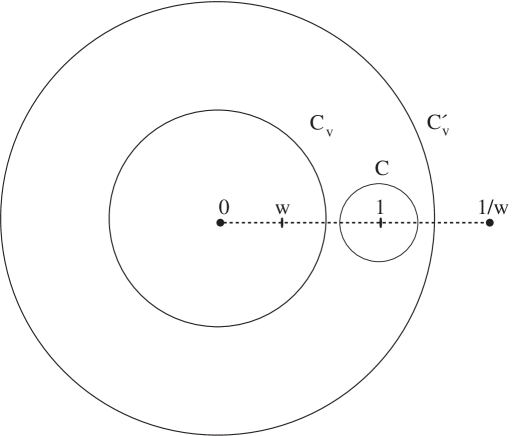
FIG. 1.: Contours used in the derivation of the recursion relation(58).

Let us consider a second $v$-contour $C_{v}^{\prime}$ defined by $1<|v^{\prime}|<|w|^{-1}$, which is related to $C_{v}$ by the transformation $v^{\prime}=w^{-1}v$. Using the properties

$$\hat{\psi}(w^{-1}v,w) = -\frac{v}{w}\hat{\psi}(v,w)$$ (51)

$$\partial_{\tau}^{n}\Omega(w^{-1}v,w) = \partial_{\tau}^{n}\Omega(v,w)$$ (52)

which follow directly from the definitions of $\hat{\psi}(v,w)$ and $\Omega(v,w)$ and taking into account the general form of the correlator (49), we may relate the two contour integrals

$$\oint_{C_{v}^{\prime}}{dv\over v}v^{n}{\langle}{V^{\prime}}^{\dagger}(k,1)\ V^{\prime}(k,v){\rangle} = w^{-n-m^{2}}\oint_{C_{v}}{dv\over v}v^{n+m^{2}}{\langle}{V^{\prime}}^{\dagger}(k,1)\ V^{\prime}(k,v){\rangle}$$ (54)

$$\ \ \ \ \ \ \ =w^{-n-m^{2}}{\mathcal{I}}_{n+m^{2}}(w)\ .$$

The difference between the two contours can be deformed into a small contour $C$ around $v=1$ (see Fig. 1), and we have

$$\left(\oint_{C_{v}^{\prime}}-\oint_{C_{v}}\right){dv\over v}v^{n}{\langle}{V^{\prime}}^{\dagger}(k,1)\ V^{\prime}(k,v){\rangle} = w^{-n-m^{2}}{\mathcal{I}}_{n+m^{2}}(w)-{\mathcal{I}}_{n}(w)$$ (56)

$$\ \ \ =\oint_{C}{dv\over v}v^{n}{\langle}{V^{\prime}}^{\dagger}(k,1)\ V^{\prime}(k,v){\rangle}\ .$$

This last integral depends only on the structure of the singularity at $v=1$, and is computed in Appendix A. Assuming that the emitted state is normalized, the result is

$$\oint_{C}{dv\over v}v^{n}{\langle}{V^{\prime}}^{\dagger}(k,1)\ V^{\prime}(k,v){\rangle}=n+\frac{m^{2}}{2}$$ (57)

and, after multiplying (56) by $w^{n+m^{2}}$, the following recursion relation is obtained

$${\mathcal{I}}_{n+m^{2}}(w)=w^{n+m^{2}}\big{[}{\mathcal{I}}_{n}(w)+n+\frac{m^{2}}{2}\big{]}\ .$$ (58)

This relation is universal, in the sense that it depends only on the mass of the emitted state. By a similar argument involving two contours related by the transformation $v^{\prime}=w/v$ the following “reflection symmetry” is easily derived

$${\mathcal{I}}_{n}(w)=w^{n}{\mathcal{I}}_{-n}(w)\ .$$ (59)

B The solutions

For photons, the recursion relation reduces to ${\mathcal{I}}_{n}(w)=w^{n}\big{[}{\mathcal{I}}_{n}(w)+n\big{]}$ with the obvious solution

$${\mathcal{I}}_{n}(w)=\frac{nw^{n}}{1-w^{n}}\ ,$$ (60)

which agrees with (14) and gives rise to the Plank distribution. For $m\neq 0$ there are no closed-form solutions, but they can be expressed as power power series in $w$. Since $\hat{\psi}(v,w)$ and all proper time derivatives of $\Omega(v,w)$ have finite limits for $w\rightarrow 0$, only positive powers of $w$ are involved. The absence of negative powers of $w$ combined with the reflection symmetry (59) implies

$${\mathcal{I}}_{n}(w)=a_{n}w^{n}+O(w^{n+1})$$ (61)

One can easily check that, for tachyons ($m^{2}=-2)$, this condition implies that the unique solution to (58) is given by the series

$${\mathcal{I}}_{n}(w)=\sum_{p=1}^{\infty}(n-1+2p)w^{(n-1)p+p^{2}}\ .$$ (62)

For positive $m^{2}=2,4,6,\ldots$ we can use (58) to express ${\mathcal{I}}_{n}(w)$ in terms of ${\mathcal{I}}_{n-m^{2}}(w)$, which in turn can be related to ${\mathcal{I}}_{n-2m^{2}}(w)$ and so on, until one reaches ${\mathcal{I}}_{\nu}(w)$, where $0\leq\nu<m^{2}$. The result of this iterative process is the following series

$${\mathcal{I}}_{n}(w)=\sum_{p=1}^{A}\Big{(}n-m^{2}(p-{1\over 2})\Big{)}w^{np-{1\over 2}m^{2}(p^{2}-p)}+{\mathcal{I}}_{\nu}(w)\,w^{\nu A+{1\over 2}m^{2}(A^{2}+A)}\ ,$$ (63)

where $\nu\equiv n\bmod{m^{2}}$ and $n=m^{2}A+\nu$. At first sight the solution (63) depends on the $m^{2}$ undetermined functions ${\mathcal{I}}_{0},\ {\mathcal{I}}_{1},\cdots{\mathcal{I}}_{m^{2}-1}$. However, combining the reflection symmetry (59) with the recursion relation yields

$${\mathcal{I}}_{\nu}(w)=w^{2\nu-m^{2}}{\mathcal{I}}_{m^{2}-\nu}(w)+\big{(}\nu-\frac{m^{2}}{2}\big{)}\,w^{\nu}\ ,$$ (64)

which implies that only ${\mathcal{I}}_{0},\ {\mathcal{I}}_{1},\cdots{\mathcal{I}}_{m^{2}/2}$ are independent functions.

Note that the structure of this solution is consistent with the fact that (58) is an inhomogeneous linear difference equation. The last piece in (63) is the general solution to the homogeneous equation ${\mathcal{I}}_{n+m^{2}}(w)=w^{n+m^{2}}{\mathcal{I}}_{n}(w)$, which exists only for $m^{2}>0$; the sum from $p=1$ to $A$ is a particular solution to the complete equation.

As mentioned above, the recursion relation is universal, in the sense that only the mass of the emitted particle enters it. However, the solutions depend on the functions ${\mathcal{I}}_{0},\ {\mathcal{I}}_{1},\cdots{\mathcal{I}}_{m^{2}/2}$, which should be determined by direct expansion of the correlator. Since this expansion depends on the particular vertex operator considered, we may say that the solution to the homogeneous equation contains the non-universal, state dependent part of the emission rate, while the particular solution reflects the universal behavior. The non-universal terms exist only for $m^{2}>0$. This is physically sensible, since there is only one tachyonic state and all $D-2$ transverse physical photon polarizations are equivalent by $SO(D-2)$ invariance.

In order to compare the relative strength of universal and non-universal contributions to the decay rate, we should note that if ${\mathcal{I}}_{n}$ is given by its power expansion ${\mathcal{I}}_{n}(w)=\sum_{l>0}a_{l}\,w^{l}$, then by (13) and (47) $F(N,N^{\prime})$ will be given by

$$F(N,N^{\prime})=\sum_{l>0}a_{l}\;{\cal G}(N\!-\!l)\ .$$ (65)

Since the degeneracy ${\cal G}(N)$ is a rapidly growing function of $N$, the higher powers of $w$ will be strongly suppressed. On the other hand, the highest power in the universal series in (63) is the term with $p=A$, which gives $l=\nu A+{1\over 2}m^{2}(A^{2}+A)$. This is precisely the power of $w$ which multiplies ${\mathcal{I}}_{\nu}(w)$ in the non-universal term and since ${\mathcal{I}}_{\nu}(w)=O(w^{\nu})$, we see that the non-universal term will tend to be suppressed in relation to the leading universal contributions. This argument fails only for $A=0$ which, as we will see in the next Section, corresponds to the emission of states carrying a large fraction of the total mass $M$.

IV Applications

In this Section we will describe some applications of the solutions to the recursion relations. Substitution of the solution (63) into (47) gives the sum over initial and final states as a linear combination of level degeneracies

$$F(N,N^{\prime})=\sum_{p=1}^{A}\Big{(}n-m^{2}(p-{1\over 2})\Big{)}{\mathcal{G}}\Big{[}N-np+{1\over 2}m^{2}(p^{2}-p)\Big{]}+F_{NU}(N,N^{\prime})\ ,$$ (66)

where $n=N-N^{\prime}$ and $F_{NU}$ is the contribution from the non-universal term

$$F_{NU}(N,N^{\prime})=\oint_{C_{w}}{dw\over w}w^{-N}f(w)^{2-D}{\mathcal{I}}_{\nu}(w)\,w^{\nu A+{1\over 2}m^{2}(A^{2}+A)}\ .$$ (67)

Note that (66) is also valid for photons and tachyons if we set $A=\infty$ and $F_{NU}=0$. The mass level degeneracies can be obtained by direct expansion of the partition function (13) or from an approximate formula, given in Appendix B, which is more accurate than the usual asymptotic expression (16).

Taking into account the normalization of the initial state and the two-body phase space, the averaged semi-inclusive decay rate is given by

$$\Gamma(M\to m+M^{\prime})=A_{D}\frac{g_{o}^{2}}{M^{2}}{F(N,N^{\prime})\over{\cal G}(N)}\,k^{D-3}\ ,$$ (68)

where

$$A_{D}=\frac{2^{-D}\pi^{\frac{3-D}{2}}}{\Gamma(\frac{D-1}{2})}$$ (69)

and $g_{o}$ is the open string coupling constant. Remember that the label “averaged semi-inclusive” refers to the fact that (68) describes the production of strings of mass $m$ in a very specific state, by typical strings of mass $M$, while summing over all final states of mass $M^{\prime}$.

A Fragmentation of heavy open strings

Here we will assume that the mass of the initial string is so large that we can use the following asymptotic approximation for the mass level degeneracies

$${\mathcal{G}}(M)\sim(2\pi T_{H})^{-\frac{D-1}{2}}M^{-\frac{D+1}{2}}e^{M/T_{H}}\ \ ,\ \ \ T_{H}=\frac{1}{\pi}\,\sqrt{\frac{3}{D-2}}\ .$$ (70)

This is (16) written in terms of the mass, and we have specified the value of the multiplicative constant in order to get quantitative results. Using (70) and

$$n=N-N^{\prime}=M\,k^{0}-{1\over 2}m^{2}\geq m(M-{1\over 2}m)\ ,$$ (71)

which follows from $p=p^{\prime}+k$ and the mass shell conditions, we can obtain the following estimate for the ratio between the first two terms in (66)

$$\frac{{\mathcal{G}}(N-2n+m^{2})}{{\mathcal{G}}(N-n)}\sim\exp\Bigg{[}-\frac{m}{T_{H}}\left(\frac{M-3m/2}{M-m}\right)\Bigg{]}\ .$$ (72)

Obviously, as long as $0<m<2M/3$ the contribution of all the terms but the first can be neglected, and we may take

$$F(N,N^{\prime})\approx(N-N^{\prime}-{1\over 2}m^{2})\ {\mathcal{G}}(N^{\prime})\ .$$ (73)

If we further asssume that $m\ll M$ we can use the approximation $n=N-N^{\prime}\approx Mk^{0}$ together with ${\mathcal{G}}(N^{\prime})/{\mathcal{G}}(N)\approx e^{-k^{0}/T_{H}}$. Then (68) implies the energy distribution

$$d\Gamma(k^{0})\approx A_{D}\,g_{o}^{2}\,e^{-k^{0}/T_{H}}k^{D-2}dk\ ,$$ (74)

where we have used $dn=Mdk^{0}$ and $k^{0}dk^{0}=kdk$. This confirms that massive strings with $m\ll M$ are radiated according to a Maxwell-Boltzmann distribution which is totally independent of the mass $M$ of the decaying string. Had we included the rest of the terms in the series in $F(N,N^{\prime})$ we would have obtained Plank distribution. But even for the lowest lying massive states $k^{0}\geq m$ is large compared with $T_{H}$, and the difference between the two distributions can be neglected.

In what follows we are going to lift the restriction $m\ll M$ and consider instead the splitting of a string of mass $M$ into arbitrary states of masses $m$ and $M^{\prime}$. Note that (68) gives the average rate of decay of a string of mass $M$ into a specific state of mass $m$. However, our approximation (73) for $F(N,N^{\prime})$ implies that all the states of a given mass level $m$ are emitted at the same rate. Thus, if we multiply the rate by ${\mathcal{G}}(m)$ the result will be the total rate for decays into arbitrary states with masses $m$ and $M^{\prime}$

$$\Gamma_{tot}(M\to m+M^{\prime})\approx A_{D}\frac{g_{o}^{2}}{M^{2}}(N-N^{\prime}-\frac{m^{2}}{2})\frac{{\mathcal{G}}(m){\mathcal{G}}(M^{\prime})}{{\mathcal{G}}(M)}\,k^{D-3}\ .$$ (75)

Note that, unlike (73), this formula is valid even for $m>2M/3$. The reason is that (75) is symmetric under interchange of the emitted strings, and at least one of the two emitted masses is going to be less than $2M/3$. The only conditions for the validity of (75) are that $M$ sould be large and neither $m$ nor $M^{\prime}$ should be zero.

As long as $m\gg 1$ and $M^{\prime}\gg 1$, we can use (70) to write

$$\frac{{\mathcal{G}}(m){\mathcal{G}}(M^{\prime})}{{\mathcal{G}}(M)}\sim(2\pi T_{H})^{-\frac{D-1}{2}}\Bigg{(}\frac{mM^{\prime}}{M}\Bigg{)}^{-\frac{D+1}{2}}e^{-t/T_{H}}\ ,$$ (76)

where $t\equiv M\!-\!m\!-\!M^{\prime}$ is the total kinetic energy or “mass deffect” for the decay. Since the exponential dependence on $t$ implies $t\sim O(T_{H})\ll M$, we can also make the following approximations

$$N-N^{\prime}-\frac{m^{2}}{2}\approx mM^{\prime}\ \ \ ,\ \ t\approx{1\over 2}\Big{(}\frac{M}{mM^{\prime}}\Big{)}\,k^{2}$$ (77)

and find for the total decay rate

$$\Gamma_{tot}(M\to m+M^{\prime})\approx A_{D}g_{o}^{2}\frac{(\pi T_{H})^{-\frac{D-1}{2}}}{2mM^{\prime}}t^{\frac{D-3}{2}}e^{-t/T_{H}}\ .$$ (78)

Thus we obtain a Maxwell-Boltzmann distribution for the total kinetic energy. Note that if we only measure the energy of one of the decay products (say the one with mass $m$) we will find a temperature

$$T_{m}=T_{H}\bigg{(}1-\frac{m}{M}\bigg{)}\ .$$ (79)

Of course, this is simply a “recoil effect”, and in the limit $m\ll M$ we recover our previous result (74). Another consequence of the distribution (78) is that the average kinetic energy released in a decay is given by

$$<t>={1\over 2}(D-1)T_{H}\ .$$ (80)

In other words, as long as neither of the final masses is too small, the energy released in the decay $M\to m+M^{\prime}$ is independent of the masses and satisfies the equipartition principle in $D-1$ spatial dimensions.

Another quantity that we may compute from (78) is the total rate of production of strings of mass $m$. We simply have to sum over all values of $N^{\prime}$ using $dN^{\prime}=-M^{\prime}dt$, and we get

$$\Gamma_{m}=\sum_{N^{\prime}}\Gamma_{tot}(M\to m+M^{\prime})\approx A_{D}g_{o}^{2}\frac{(\pi T_{H})^{-\frac{D-1}{2}}}{2m}\int_{0}^{\infty}\textrm{d}tt^{\frac{D-3}{2}}e^{-t/T_{H}}=\frac{A^{\prime}_{D}g_{o}^{2}}{m}\ ,$$ (81)

where $A^{\prime}_{D}=\pi^{2-D}2^{-(D+1)}$. In terms of the level density $\rho(m)\!=\!m$, which follows from the mass shell condition, there are $\rho(m)\,dm$ levels with masses between $m$ and $m+dm$. Thus the number of particles produced within that interval is given by the density

$$\frac{\textrm{d}\Gamma(m)}{\textrm{d}m}=\Gamma_{m}\,\rho(m)\approx A^{\prime}_{D}g_{o}^{2}\ ,$$ (82)

which is independent of the masses. This means that a heavy open string radiates strings of all masses with equal probabilities and implies a total decay rate proportional to the mass of the string. Thus, the decay of a heavy open string can be described as a process of fragmentation, rather than one of radiation.

From a semiclassical point of view, this can be explained in terms of a constant splitting probability per unit of length [3, 4]. Since the released energy (80) is small compared to the masses, $M\approx m+M^{\prime}$ and all masses smaller than $M$ are produced with the same probability. This should fail when one of the masses is comparable to the released energy. From the point of view of our computation, this failure can be attributed to the breakdown of the asymptotic approximation for the level multiplicity.

The total decay rate of a string of mass $M$ is obtained by integrating (82) from $0$ to $M/2$, to avoid counting each decay mode twice. The result for $D=26$ is $g_{o}^{2}\pi^{-24}2^{-28}M$ and can be compared to other computations in the literature. The decay rate for open bosonic strings on the leading trajectory is given by eq. (12) of [3] and exactly agrees with ours. They obtain their result from the one-loop planar diagram, which is equivalent to considering only one cyclic ordering for the three-point tree amplitude. Including the non-planar contribution as in [12] amounts to adding the other cyclic ordering, but the result is easy to predict. As mentioned in Section 2, amplitudes for $U(1)$ strings vanish or get a factor of $2$ depending on the parity of $N+N_{1}+N_{2}$. The net result is that the total decay rate should be multiplied by $2$, yielding $g_{o}^{2}\pi^{-24}2^{-27}M$. This can also be compared with the decay rate for a long straight open string , which according to eq. (14) of [4] is given by $g_{o}^{2}\pi^{-24}2^{-26}M$. This is twice our result, but the discrepancy may be due to some overlooked subtlety. In any case, since we are computing the averaged decay rate for strings of mass $M$, the result need not coincide with those obtained for highly atypical states such as those on the leading Regge trajectory.

We can also use (75) to compute the production rate $\Gamma_{m}$ by strings of mass $M$ numerically and compare the results with the asymptotic prediction (82). Fig. 2 shows our results for $N=20$ and $N=100$ in $26$ dimensions, with $\frac{d\Gamma(m)}{dm}$ normalized so that $1$ corresponds to the asymptotic value (82). Note that even for $N$ as low as $20$ the rate manages to attain the predicted value for $m\approx 2.3$ and that for $N=100$ there is already a well defined plateau, with a decrease in the rate near the ends of the mass range.

FIG. 2.: $\frac{d\Gamma(m)}{dm}$ for $D=26$, $N=20$ ($M\approx 6.16$, left) and $N=100$ ($M\approx 14.1$, right).

For $D\neq 26$ the results do not match (82) so well. For $D<26$ the production of light strings is enhanced, while the opposite is true for $D>26$. This is illustrated in Fig. 3, which suggests that strings decay according to a the constant splitting probability only in $26$ dimensions [3]. However, one should not forget that the consistency of the formalism is suspect for $D\neq 26$. Since ${\mathcal{G}}(N)$ does not count the total number of propagating states for $D<26$, and for $D>26$ there are also negative norm physical states, the validity of (75) for $D\neq 26$ is unclear.

FIG. 3.: $\frac{d\Gamma(m)}{dm}$ for $N=500$ and $D=16$ (left), $D=26$ (center) and $D=30$ (right).

B Radiation by heavy closed strings

Our previous computations extend easily to the case of heavy closed strings but, as we shall see, the results are remarkably different. Tree amplitudes for closed strings factorize into a product of left and right open string amplitudes , and instead of (68) we have

$$\Gamma_{c}(M\to m+M^{\prime})=A_{D}\frac{g_{c}^{2}}{M^{2}}{F(N,N^{\prime})^{2}\over{\cal G}(N)^{2}}\,k^{D-3}\ ,$$ (83)

where $g_{c}$ is the closed string coupling constant, which is proportional to $g_{o}^{2}$. For closed strings, the mass shell condition becomes $\alpha^{\prime}M^{2}=4(N-1)$, and this introduces numerical factors into some of the previous formulas. For instance, eq. (71) becomes

$$n=N-N^{\prime}=\frac{1}{4}\big{(}M\,k^{0}-{1\over 2}m^{2}\big{)}\ .$$ (84)

The computations proceed along the same lines and we will merely quote the main results. For $m\ll M$ the energy distribution of emitted strings is given by

$$d\Gamma_{c}(k^{0})\approx\frac{1}{64}A_{D}\,g_{c}^{2}M\,k^{0}e^{-k^{0}/T_{H}}\,k^{D-2}dk\ .$$ (85)

Besides the trivial numerical factor, there are two important differences with the analogous formula (74) for open strings. These are the presence of the mass $M$ and the factor $k^{0}$. The latter can be seen as a grey body correction to black body spectrum, similar to the ones found in other contexts [11]. The factor of $M$ indicates that, unlike open strings, closed strings radiate proportionally to their mass.

Even more striking is the difference regarding the total emission rate of strings of mass $m$. Instead of (82) we find

$$\frac{\textrm{d}\Gamma_{c}(m)}{\textrm{d}m}\approx A^{\prime\prime}_{D}\,g_{c}^{2}M\,m_{R}^{-\frac{D-1}{2}}\ ,$$ (86)

where $m_{R}\equiv m(M-m)/M$ and $A^{\prime\prime}_{D}=2^{-\frac{D+15}{2}}\,\pi^{-\frac{3D-5}{2}}T_{H}^{-\frac{D-1}{2}}$. The power of $m_{R}$ implies that light strings are produced much more copiously than heavy ones. However, the factor of $M$ guarantees that the lifetime is proportional to $M^{-1}$, as for open strings. Similarly, the mean kinetic energy released per decay is still given by (80).

As in the case of open strings, there is a simple semiclassical interpretation for (86), at least in the limit $1\ll m\ll M$. In order for the initial string to split, one point 1 has to touch a second point 2. The point 1 can be anywhere along the length $L$ of the string, and this explains the factor of $M\sim L$. Between 1 and 2 there is a piece of string of length $l\sim m$, and if we assume that the string shape is that of a random walk [22, 18], the mean distance between the two points will be $\sim m^{1/2}$. The probability for the two points to meet is inversely proportional the corresponding volume $m^{(D-1)/2}$ in $D-1$ space dimensions. For $m\ll M$, $m_{R}\approx m$, and this explains the mass dependence in (86).

C Decays of light strings

By “light strings” we actually mean those with $M^{2}=2(N-1)$ not large enough to use asymptotic approximations for the decay rates. Then some of the results obtained for heavy strings may no longer be valid. Such is the case with the energy distributions (74), (78) and (85), and with the production rates (82) and (86). However, other formulas do not rely on the asymptotic approximation (70) for the mass degeneracies and may still be valid for $N$ in the tens or hundreds, depending on the level of precission sought. This is true of eqs. (73) and (75).

On the other hand, for small values of $N$ one can obtain exact results by summing the whole series in (66). A simple example which serves to illustrate the fact, mentioned in Section 2, that $F(N,N^{\prime})$ counts “longitudinal” states for $D<26$ is the decay $2\rightarrow 1+1$ of the symmetric rank-two tensor (35) into two photons. For photon production by light strings, one simply uses (66) with $F_{NU}=0$, getting

$$F(2,1)={\mathcal{G}}(1)+{\mathcal{G}}(0)=(D-2)+1=D-1\ .$$ (87)

This case is so simple that we can compute the amplitudes by hand and sum the probabilities over all the polarizations of the tensor and remaining photon according to the definition (4) of $F(N,N^{\prime})$. We find

$$D-1-\frac{26-D}{8(D-1)}\ ,$$ (88)

which agrees with (87) only for $D=26$. The reason for the discrepancy is the following. At the critical dimension the only propagating physical state at mass level two is the rank-two symmmetric tensor. However, the “longitudinal” state [13]

$$|\phi{\rangle}=[\alpha_{-1}\cdot\alpha_{-1}+\frac{D-1}{5}p\cdot\alpha_{-2}+\frac{D+1}{10}(p\cdot\alpha_{-1})^{2}]|p{\rangle}\ \ \ ,\ \ -p^{2}=m^{2}=2$$ (89)

satisfies the Virasoro conditions and has positive norm for $D<26$

$${\langle}\phi|\phi{\rangle}=\frac{2}{25}(D-1)(26-D)\ .$$ (90)

The decay of this state into two photons gives a contribution $(26-D)/8(D-1)$ which exactly cancels the discrepancy. This example shows that, for $D<26$, the double sum $F(N,N^{\prime})$ includes states which are not simply obtained by truncation of the $D=26$ spectrum.

For emission of states with $m^{2}>0$ we must determine ${\mathcal{I}}_{\nu}(w)$ by direct expansion of the two point-function in powers of $v$ and $w$. Fortunatelly, we only need to compute a few terms in the expansion. The reason is that the degeneracies vanish for negative arguments, and by (67) and (61) the non-universal contribution takes the form

$$F_{NU}(N,N^{\prime})=a_{\nu}\,{\mathcal{G}}\Big{[}N-\nu(A+1)-{1\over 2}m^{2}(A^{2}+A)\Big{]}+\ldots$$ (91)

One can easily show that

$$\max\Big{[}N-\nu(A+1)-{1\over 2}m^{2}(A^{2}+A)\Big{]}=1+\textrm{Int}(\frac{m^{2}}{8})\ ,$$ (92)

so that ${\mathcal{I}}_{\nu}(w)$ must be known only throught order $O(w^{\nu+1+Int(m^{2}/8)})$. One can also show that the limit (92) is approached only for some “soft” decays with very little kinetic energy, i.e. with $M\approx m+M^{\prime}$, and that for most decay modes the non-universal contribution vanishes because the lowest power of $w$ in ${\mathcal{I}}_{\nu}(w)\,w^{\nu A+{1\over 2}m^{2}(A^{2}+A)}$ is greater than $N$.

Since the leading universal term in (66) is proportional to ${\mathcal{G}}(N^{\prime})={\mathcal{G}}(1+M^{\prime 2}/2)$, whereas by (92) the leading non-universal term is, at best, proportional to ${\mathcal{G}}(1+m^{2}/8)$, non-universal terms are important only for soft decays with $m\approx 2M^{\prime}\approx 2M/3$ or greater. Indeed, for $m>2M/3$, $A=0$ in (66) and $F(N,N^{\prime})=F_{NU}(N,N^{\prime})$. This is not surprising, since for $m\geq 2M/3$ the “emitted string” is more appropriately described as a “remnant”, and the rate is expected to depend on its particular state.

Most decay modes are accurately described by the universal series in (66) and, since this is a rapidly decreasing series, it is often enough to keep the first few terms. Moreover, there are even decay modes for which only the first term in the series is non-zero. For $M^{2}>2\,(m^{2}+M^{\prime 2}+1)$ the argument of ${\mathcal{G}}$ for the second term in (66) is already negative and the following formula is exact

$$F(N,N^{\prime})=(N-N^{\prime}-{1\over 2}m^{2})\,{\mathcal{G}}(N^{\prime})\ .$$ (93)

As an illustration of these general remarks we will consider the production of $m^{2}=2$ states, i.e. decays of the form $N\to 2+N^{\prime}$. Here we will work at the critical dimension $D=26$. In this case there are non-universal contributions and we must first compute ${\mathcal{I}}_{0}(w)$ and ${\mathcal{I}}_{1}(w)$ from (37). The result is

$${\mathcal{I}}_{0}(w) = (1+8w)(\xi_{\mu\nu}p^{\mu}p^{\nu})^{2}-16w\,(\xi_{\mu\rho}\xi_{\nu}^{\ \ \rho}p^{\mu}p^{\nu})+4w\,(\xi_{\mu\nu}\xi^{\mu\nu})+O(w^{2})$$ (94)

$${\mathcal{I}}_{1}(w) = -2(w+6w^{2})\,(\xi_{\mu\nu}p^{\mu}p^{\nu})^{2}+4(w+6w^{2})\,(\xi_{\mu\rho}\xi_{\nu}^{\ \ \rho}p^{\mu}p^{\nu})-4w^{2}\,(\xi_{\mu\nu}\xi^{\mu\nu})+O(w^{3})\$$ (95)

where, following the analysis around eq. (92), we have included terms of order $w$ and $w^{2}$ respectively. The values of the Lorentz invariants for different polarizations of the emitted tensor are given in Table I, where the components are referred to the emitted tensor rest frame, $1$ is the direction in which the tensor is emitted, and $a,b=2,3,\ldots,25$.

Polarization $\ (\xi_{\mu\nu}p^{\mu}p^{\nu})^{2}\$ $\ \xi_{\mu\rho}\xi_{\nu}^{\ \ \rho}p^{\mu}p^{\nu}\$ $\ \xi_{\mu\nu}\xi^{\mu\nu}\$ $\xi_{ab}$ $0$ $0$ $\frac{1}{2}$ $\xi_{1a}$ $0$ $\frac{1}{4}x$ $\frac{1}{2}$ $\xi_{11}$ $\frac{12}{25}x^{2}$ $\frac{12}{25}x$ $\frac{1}{2}$

TABLE I. Values to be used in (94) with $x=(1+n)^{2}/2-M^{2}$.

For example, for $7\to 2+3$ we have $n=7-3=4$ and (63) gives

$${\mathcal{I}}_{4}(w)=3w^{4}+w^{6}+w^{6}{\mathcal{I}}_{0}(w)$$ (96)

which, using Table I with $x={1\over 2}$ yields

$$F(7,3)=3{\mathcal{G}}(3)+{\mathcal{G}}(1)+\left\{\begin{array}[]{lll}2\ \ =\ \ 9626&\ \ \textrm{for}&\xi_{ab}\\ 0\ \ =\ \ 9624&\ \ \textrm{for}&\xi_{a1}\\ 2\ \ =\ \ 9626&\ \ \textrm{for}&\xi_{11}\ \ .\end{array}\right.$$ (97)

The other possible non-tachyonic decay modes of the form $7\to 2+N^{\prime}$ are $7\to 2+2$ and $7\to 2+1$. The corresponding sums are universal and given by

$${\mathcal{I}}_{5}(w) = 4w^{5}+O(w^{8})\ \ \ ,\ \ \ F(7,2)=4\,{\mathcal{G}}(2)=1296$$ (98)

$$\ {\mathcal{I}}_{6}(w) = 5w^{6}+O(w^{10})\ \ ,\ \ \ F(7,1)=5\,{\mathcal{G}}(1)=120\ \ \ \ .$$ (99)

Note that out of the three decay modes only $7\to 2+3$, which is the one with the smallest kinetic energy, has non-universal contributions and that these are very small, of the order of $0.02\%$. A similar computation for $3\to 2+1$ and $4\to 2+1$ yields non-universal contributions of $8\%$ and $4\%$ respectively. This confirms that these contributions are significant only when the emitted particle carries a large fraction of the original mass. Also note that the relative contribution of the second term in (97) is rather small, of the order of $0.25\%$. Similar examples show that (75), which uses only the first term in the solution, gives very accurate results for $N$ as low as $10$ or $20$.

V Discussion

In this paper we have considered the problem of computing the averaged semi-inclusive rates for emission of specific string states of mass $m$. This requires the evaluation of the double sum

$$F(N,N^{\prime})=\sum_{\Phi_{i}|_{N}}\sum_{\Phi_{f}|_{N^{\prime}}}\big{|}\langle\Phi_{f}|V(k)|\Phi_{i}\rangle\big{|}^{2}\ ,$$ (100)

where $V(k)$ is the vertex operator for a string state of mass $m$. Our solution involves a recursion relation (58) which is a linear difference equation and depends only on the mass $m$ of the emitted string, with the details of the specific emitted state entering only as “initial conditions”. The universal series in the solution (63)

$${\mathcal{I}}_{n}(w)=\sum_{p=1}^{A}\Big{(}n-m^{2}(p-{1\over 2})\Big{)}w^{np-{1\over 2}m^{2}(p^{2}-p)}+\ldots$$ (101)

suggests some sort of “deformation” of Plank’s distribution for massless strings

$${\mathcal{I}}_{n}(w)=\frac{nw^{n}}{1-w^{n}}=\sum_{p=1}^{\infty}n\,w^{np}\ .$$ (102)

It would be interesting to check if this series is truly universal and appears in other averaged semi-inclusive quantities such as $N$-point functions, or is just particular to the $3$-point functions considered here.

Being able to compute averaged semi-inclusive $4$-point functions would also be interesting in its own right. They would give us the “form factors” of typical fundamental strings, with direct information on their shape and size. This would be an alternative approach, along the lines of [23], to the one pursued in [18] for the determination of the sizes of fundamental strings [24]. One could also try to compare the form factors with the scattering properties of black holes, and see it some of them can be adscribed to a “decoherence” process [16].

Our analysis has shown that the decoherence procedure of averarging over all initial states of mass $M$ is very efficient in suppressing the dependence on the state of the emitted string, unless this string carries a very substantial fraction of the original mass. In fact, most decay modes are well described by the first term in the universal series. Dividing the approximate expression (73) for $F(N,N^{\prime})$ by ${\mathcal{G}}(N){\mathcal{G}}(N^{\prime})$ yields the “averaged interaction rate”

$$<\big{|}\langle\Phi_{f}|V(k)|\Phi_{i}\rangle\big{|}^{2}\!>\approx(N-N^{\prime}-{1\over 2}m^{2})\frac{1}{{\mathcal{G}}(N)}=\frac{k\cdot p^{\prime}}{{\mathcal{G}}(N)}$$ (103)

for the reaction $M\to m+M^{\prime}$ with $p=k+p^{\prime}$. Note that in this case we have averaged over the three strings involved. For closed strings the result is similar

$$<\big{|}\langle\Phi_{f}|V(k)|\Phi_{i}\rangle\big{|}^{2}\!>\approx\frac{(k\cdot p^{\prime})^{2}}{{\mathcal{G}}(N)^{2}}$$ (104)

and was obtained in [10] by a different method. These results are very simple, and suggest that similar simplifications might take place for higher order interactions.

Our results for the production rates of strings of mass $m$ by heavy open and closed strings

$$\frac{\textrm{d}\Gamma_{o}(m)}{\textrm{d}m}=A^{\prime}_{D}g_{o}^{2}\ \ ,\ \ \frac{\textrm{d}\Gamma_{c}(m)}{\textrm{d}m}=A^{\prime\prime}_{D}\,g_{c}^{2}M\,m_{R}^{-\frac{D-1}{2}}\ \ ,\ \ m_{R}\equiv\frac{m(M-m)}{M}$$ (105)

have very simple semiclassical interpretations and provide a microscopic basis for the type of heuristic interactions used in the Boltzmann equation approach to hot string gases [8, 9]. In particular, the small value of the mean kinetic energy obtained in (80) gives support to the assumption that the total length of the strings is approximately conserved. It is interesting that the mass dependences in (105), which from a semiclassical viewpoint are a consequence of the random walk structure of long strings, arise microscopically as a result of the interplay between mass degeneracies and phase space factors. Their effects cancel out for open strings, giving rise to a flat spectrum. The decay rates for typical open strings computed in this paper agree, within a factor of $2$, with those computed for strings in very special states [3, 4].

For open strings on a Dp-brane the spectrum is no longer flat. The string can oscillate in $D$ dimensions, but its endpoints are bound to a $p+1$ manifold. The phase space factor in (75) becomes $k^{p-2}$, and instead of a flat spectrum we find a rate proportional to $m_{R}^{-d/2}$, where $d\equiv D-p-1$ is the number of “extra dimensions” orthogonal to the brane. This may be relevant to the decays of “string balls” in brane-world scenarios [19]. It would be interesting to study the decay properties of strings in other situations involving D-branes, such as those considered in [6, 9]. Another possible extensions along these lines would be to include the effect of external fields and non-conmutative limits of the theory [7] on the decay rates.

ACKNOWLEDGMENTS

It is a pleasure to thank J.M. Aguirregabiria, I.L. Egusquiza, R. Emparan, Jaume Gomis, Joaquim Gomis, M.A. Valle-Basagoiti and M.A. Vázquez-Mozo for useful and interesting discussions. This work has been supported in part by the Spanish Science Ministry under Grant AEN99-0315 and by a University of the Basque Country Grant UPV-EHU-063.310-EB187/98.

A

Here we will compute the integral (57) which appears in the derivation of the recursion relation. The scalar two-point function on the cylinder $\psi(v,w)$ is related to the Jacobi $\vartheta_{1}$ function by[13]

$$\psi(v,w)=\frac{2\pi i}{\tilde{\tau}}\,\frac{\vartheta_{1}(\nu|\tilde{\tau})}{\vartheta^{\prime}_{1}(0|\tilde{\tau})}\ \ \ ,\ \ \tilde{\tau}\equiv-\frac{2\pi i}{\ln w},\ \ \ ,\ \ \nu\equiv\frac{\ln v}{\ln w}$$ (A1)

and using the product formula for the theta function yields the following expression

$$\psi(v,w)=-\frac{2\pi}{\ln q}\sin\pi\nu\prod_{1}^{\infty}\frac{1-2q^{2n}\cos 2\pi\nu+q^{4n}}{(1-q^{2n})^{2}}\ ,$$ (A2)

where $q=e^{i\pi\tilde{\tau}}$. The function $\psi(v,w)$ has zeroes for $v=w^{n}$ with $n=0,\pm 1,\pm 2,\ldots$, and expanding (A2) around $v=1$ gives

$$\psi(v,w)=-\ln(v)+O((\ln v)^{3})=-\tau+O(\tau^{3})\ ,$$ (A3)

where $\tau$ is the euclidean proper time used throughout the paper and should not be confused with the modular parameter $\tilde{\tau}$ in (A1). This fixes the behavior of the function $\hat{\psi}(v,w)$ near $v=1$

$$\hat{\psi}(v,w)=\sqrt{v}\exp\left({-\ln^{2}v\over 2\ln w}\right)\,\psi(v,w)=-\tau(1+{1\over 2}\tau)+O(\tau^{3})$$ (A4)

and implies

$${\langle}e^{-ik.X_{o}(1)}e^{ik.X_{o}(v)}{\rangle} = \hat{\psi}(v,w)^{m^{2}}=\tau^{m^{2}}\Big{(}1+\frac{m^{2}}{2}\tau+O(\tau^{2})\Big{)}$$ (A5)

$${\langle}\partial_{\tau}X^{\mu}_{o}(1)\partial_{\tau}X^{\nu}_{o}(v){\rangle} = \eta^{\mu\nu}\partial^{2}_{\tau}\ln\hat{\psi}(v,w)=-\Omega(v,w)=-\frac{1}{\tau^{2}}+O(1)\ .$$ (A6)

Each additional proper time derivative contributes a negative power of $\tau$, and (A5) together with the mass shell condition implies the following form for the correlator

$${\langle}{V^{\prime}}^{\dagger}(k,1)\ V^{\prime}(k,v){\rangle}=\frac{A}{\tau^{2}}(1+\frac{m^{2}}{2}\tau)+O(1)\ .$$ (A7)

The value of $A$ can be found by noting that computing the leading singularity of the correlator with the help of (A5) is equivalent to finding the leading term in the OPE of ordinary (unprimed) vertex operators. But this term is given by

$$V_{i}^{\dagger}(0)V_{j}(\tau)=\frac{{\langle}{\langle}\bar{i}|j{\rangle}}{\tau^{2}}+\ldots$$ (A8)

where ${\langle}{\langle}\bar{i}|j{\rangle}$ is essentially Zamolodchikov’s inner product, which is related to the familiar quantum mechanical inner product by ${\langle}{\langle}\bar{i}|j{\rangle}={\langle}{i}|j{\rangle}$. Comparing (A7) and (A8) implies $A=1$ for normalized states. Computing the integral gives

$$\oint_{C}\frac{dv}{v}v^{n}{\langle}{V^{\prime}}^{\dagger}(k,1)\ V^{\prime}(k,v){\rangle}=\oint_{0}d\tau e^{n\tau}\frac{1}{\tau^{2}}(1+\frac{m^{2}}{2}\tau)=n+\frac{m^{2}}{2}\ .$$ (A9)

B

In this Appendix we present an approximate expression for the mass level degeneracy which is more accurate than the usual asymptotic formula (70). We have used it in our numerical computations in Section 5, and find it particularly useful for the range of values of $N$ where a direct power expansion of the partition function is not practical, while the asymptotic formula is not yet accurate enough.

The basic idea is to compute the first corrections to the saddle-point aproximation for

$${\mathcal{G}}(N,D)=\oint\frac{dw}{w}w^{-N}f(w)^{2-D}\ \ \ ,\ \ \ f(w)=\prod_{n=1}^{\infty}(1-w^{n})\ .$$ (B1)

Since the saddle-point is close to $w=1$, one has to use the modular transformation

$$f(w)=\bigg{(}\frac{-2\pi}{\ln w}\bigg{)}^{1/2}w^{-1/24}q^{1/12}f(q^{2})\ \ \ ,\ \ \ q\equiv e^{2\pi^{2}/\ln w}$$ (B2)

which gives

$$\ln f(w)={1\over 2}\ln 2\pi-{1\over 2}\ln\beta+\frac{1}{24}\beta-\frac{\pi^{2}}{6\beta}+O\big{(}e^{-4\pi^{2}/\beta})$$ (B3)

where we have made the change of variable $w=e^{-\beta}$. Keeping all corrections of order $O(N^{-1/2})$ yields the following result

$${\mathcal{G}}(N,D)\sim\Big{(}\frac{24}{D-2}\Big{)}^{1/2}\frac{e^{a(x)}}{(2\pi b(x))^{1/2}}\Bigg{(}1+\frac{c(x)}{D-2}\Bigg{)}\ ,$$ (B4)

where

$$a(x) \equiv (N-\frac{D-2}{24})\frac{1}{x}+\frac{D-2}{24}\Big{(}4\pi^{2}x-12\ln x-12\ln 2\pi\Big{)}$$ (B5)

$$b(x) \equiv 4x^{2}(2\pi^{2}x-3)$$ (B6)

$$c(x) \equiv \frac{9}{2}\frac{4\pi^{2}x-3}{(2\pi^{2}x-3)^{2}}-\frac{45(\pi^{2}x-1)^{2}}{(2\pi^{2}x-3)^{3}}$$ (B7)

and the position of the saddle-point is given by

$$x\equiv\frac{1}{\beta_{0}}=\frac{1}{2\pi^{2}}\Bigg{\{}3+\sqrt{9+\pi^{2}\Big{(}\frac{24N}{D-2}-1\Big{)}}\Bigg{\}}\ .$$ (B8)

The following table gives a few sample values for the degeneracies, and we can compare the exact results for ${\mathcal{G}}(N,D)$ with those obtained from (B4). Note that the agreement is very good for $N$ as low as $20$, and even the results for $N=1$ are acceptable.

    N ${\mathcal{G}}(N,26)$ (B4) ${\mathcal{G}}(N,16)$ (B4) $1$ $24$ $23.819$ $14$ $13.949$ $5$ $176,256$ $176,271$ $19,754$ $19,759$ $20$ $\ 2.16109\cdot 10^{14}\$ $\ 2.16118\cdot 10^{14}\$ $\ 3.41780\cdot 10^{11}\$ $\ 3.41806\cdot 10^{11}\$ $100$ $2.43478\cdot 10^{40}$ $2.43480\cdot 10^{40}$ $7.90265\cdot 10^{31}$ $7.90276\cdot 10^{31}$

TABLE II. Sample values of ${\mathcal{G}}(N,D)$

This should be compared with the usual asymptotic approximation

$${\mathcal{G}}(M)\sim(2\pi T_{H})^{-\frac{D-1}{2}}M^{-\frac{D+1}{2}}e^{M/T_{H}}\ \ ,\ \ \ T_{H}=\frac{1}{\pi}\,\sqrt{\frac{3}{D-2}}$$ (B9)

which, for $N=100$, gives $4.79\cdot 10^{40}$ for $D=26$ and $9.20\cdot 10^{31}$ for $D=16$.

REFERENCES

-
[1]
M.B. Green and G. Veneziano, Phys. Lett. B36 (1971)
477.
D. Mitchell, N. Turok, R. Wilkinson and P. Jetzer, Nucl. Phys. B315 (1989) 1.
R. Wilkinson, N. Turok and D. Mitchell, Nucl. Phys. B332 (1990) 131. -
[2]
H. Okada and A. Tsuchiya, Phys. Lett. B232 (1989) 91.
A. Tsuchiya and A. Okada, Phys. Rev. Lett. 65 (1990) 397.
Y. Leblanc and A. Tsuchiya, Int. Jour. Mod. Phys. A7 (1992) 6313. - [3] D. Mitchell, B. Sundborg and N. Turok, Nucl. Phys. B335 (1990) 621.
- [4] J. Dai and J. Polchinski, Phys. Lett. B220 (1989) 387.
-
[5]
J.J. Attick and E. Witten, Nucl. Phys. B310 (1988)
291.
N. Deo, S. Jain, C.-I. Tan, Phys. Rev. D40 (1989) 2626.
M.J. Bowick and S.B. Giddings, Nucl. Phys. B325 (1989) 631.
N. Deo, S. Jain, C.-I. Tan, Phys. Lett. B220 (1989) 125. -
[6]
M.B. Green, Phys. Lett. B282 (1992) 380
[hep-th/9201054]
S.A. Abel, J.L.F. Barbón, I.I. Kogan and E. Rabinovici, JHEP 9904 (1999) 015 [hep-th/9902058].
M.A. Vázquez-Mozo, Phys. Lett.B388 (1996) 494 [hep-th/9607052] -
[7]
A.A. Tseytlin, Nucl. Phys. B524 (1998) 41
[hep-th/9802133].
E.J. Ferrer, E.S. Fradkin and V. de la Incera, Phys. Lett. B248 (1990) 281.
J. Gomis, M. Kleban, T. Mehen, M. Rangamani and S. Shenker, JHEP 0008 (2000) 011 [hep-th/0003215].
S.S. Gubser, S. Gukov, I.R. Klebanov, M. Rangamani and E. Witten, hep-th/0009140.
J. Gomis and H. Ooguri, hep-th/0009181.
J. Ambjørn, Y.Y. Makeenko, G.W. Semenoff and R.J. Szabo, hep-th/0012092. -
[8]
P. Salomonson and B. Skagerstam, Nucl. Phys. B268
(1986) 349.
F. Lizzi and I. Senda, Phys. Lett. B244 (1990) 27.
F. Lizzi and I. Senda, Nucl. Phys. B359 (1991) 441.
D.A. Lowe and L. Thorlacius, Phys. Rev, D51 (1995) 665 [hep-th/9408134]. - [9] S. Lee and L. Thorlacius, Phys. Lett. B413 (1997) 303 [hep-th/9707167].
- [10] F. Lizzi and I. Senda, Phys. Lett. B246 (1990) 385.
- [11] J.M. Maldacena and A. Strominger, Phys. Rev. D55 (1997) 861 [hep-th/9609026].
- [12] D. Amati and J.G. Russo, Phys. Lett. B454 (1999) 207 [hep-th/9901092].
- [13] M. Green, J. Schwarz and E. Witten, Superstring Theory, Vols. I and II, (Cambridge 1987).
- [14] J. Polchinski, String Theory, Vols. I and II, (Cambridge 1998).
- [15] R. Hagedorn, Nuovo Cim. Suppl. 3 (1965) 147
-
[16]
R. Myers, Gen. Rel. Grav. 29 (1997) 1217 [gr-qc/9705065].
D. Amati, hep-th/9706157, gr-qc/0103073. - [17] G.T. Horowitz and J. Polchinsky, Phys. Rev. D55 (1997) 6189 [hep-th/9612146].
- [18] T. Damour and G. Veneziano, Nucl. Phys. B568 (2000) 93 [hep-th/9907030].
- [19] S. Dimopoulos and R. Emparan, hep-ph/0108060.
- [20] A.M. Polyakov, Gauge Fields and Strings, (Harwood Ac. Pub. 1987).
- [21] J.L. Mañes and M.A.H. Vozmediano, Nucl. Phys. B236 (1989) 271.
- [22] D. Mitchell and N. Turok, Nucl. Phys. B294 (1987) 1138.
- [23] D. Mitchell and Bo Sundborg, Nucl. Phys. B349 (1991) 159.
- [24] M. Karliner, I. Klebanov and L. Susskind, Int. J. Mod. Phys. A3 (1988) 1981.