Localisation of massive fermions on the brane

Abstract

We construct an explicit model to describe fermions confined on a four dimensional brane embedded in a five dimensional anti-de Sitter spacetime. We extend previous works to accommodate massive bound states on the brane and exhibit the transverse structure of the fermionic fields. We estimate analytically and calculate numerically the fermion mass spectrum on the brane, which we show to be discrete. The confinement life-time of the bound states is evaluated, and it is shown that existing constraints can be made compatible with the existence of massive fermions trapped on the brane for durations much longer than the age of the Universe.

I Introduction

The idea that our universe may be a hypermembrane in a five dimensional spacetime has received some attention in the last few years after it was realized that gravity could be localized on a three-brane embedded in an anti-de Sitter spacetime [1]. Since then, much work has been done in a cosmological context [2] and there is hope that a consistent (i.e., mathematically self-contained and observationally satisfying) high dimensional model might soon be formulated. For instance, it has been proposed that a model [3] based on such ideas could present itself as an alternative to the inflationary paradigm, although for the time being the controversy as to whether or not such a model might have anything in common with our Universe is still going on [4].

The idea is not new however, but has evolved from the standard Kaluza-Klein approach to that of particle localization on a higher dimensional defect [5, 6]. In particular, it has been shown that massless bulk scalars and gravitons share the property to have a zero mode localized on the brane [7] in the Randall-Sundrum model. Various mechanisms [8] have been invoked according to which it would be possible to confine massless gauge bosons on a brane, so that there is hope to achieve a reasonable model including all the known interactions in a purely four dimensional effective model.

A mechanism permitting localization of massless fermions on a domain wall was described in Refs. [5, 9]. However, although appealing this mechanism might be, it should be emphasized that actual fermions, as seen on an everyday basis in whatever particle physics experiment, are massive, so that a realistic fermionic matter model on the brane must accommodate for such a mass. The question of localization of massive fermions on the brane thus arises naturally, and it is the purpose of this work to provide the transverse brane and fermionic structure that leads to this localization. Up to now, fermions have been confined under the restricting hypothesis that the brane self gravity was negligible [10], or that it was embedded in a Minkowski spacetime with one [11] or two [12] transverse dimensions (see also [13] for the localization of fermion on a string-like defect in five dimension).

Our goal is to transpose the original work of Ref. [12] to the brane context. For that purpose, we realize the brane as a domain wall. Such domain wall configurations in anti-de Sitter space have already been studied [14, 15]. We will assume that five dimensional fermions are Yukawa-coupled to the domain wall forming Higgs field, as in the usual case of cosmic strings. In this respect, our work somehow extends Ref. [10], where the mass term was put by hand, and Ref. [11] where the gravity of the wall was neglected.

We start, in the following section, by recalling the domain wall configuration of a Higgs field in a five dimensional anti-de Sitter spacetime and discuss briefly its properties. In section III, we describe the dynamical equations of fermions coupled to this domain wall in order to show that they obey a Schrödinger-like equation with an effective potential which can trap massive modes on the wall. The asymptotic structure, i.e., deep in the bulk (far from the brane), is not Minkowski space, so that the effective potential felt by the fermions possesses a local minimum at the brane location, but no global minimum, as first pointed out in Ref. [10]. As a consequence, the bound states are metastable and fermions can tunnel to the bulk.

We then provide an analytical approximation of the effective potential, thanks to which we compute analytically, in section IV, the mass spectrum of the fermions trapped on the brane. We obtain the mass of the heaviest fermion that can live on the brane and estimate its tunneling rate. This result is compared to a full numerical integration, performed in section V. In a last section, we investigate the parameter space and, after having compared our results to previous ones, we conclude that there exists a wide region in the parameter space for which the fermion masses can be made arbitrary low, i.e., comparable to the observed small values (with respect to the brane characteristic energy scale), while their confinement life-time can be made much larger than the age of the Universe. Such models can therefore be made viable as describing realistic matter on the brane.

II Membrane configuration in AdS₅

We consider the action for a real scalar field $\Phi$ coupled to gravity in a five dimensional spacetime

$$S=\int\left[\frac{1}{2\kappa_{{}_{5}}^{2}}(R-2\Lambda)+\frac{1}{2}g^{AB}\partial_{A}\Phi\partial_{B}\Phi-V(\Phi)\right]\sqrt{g}\,{\rm d}^{5}x\equiv\int\sqrt{g}\,{\rm d}^{5}x[{\cal L}_{{}_{\rm grav}}+{\cal L}_{\Lambda}+{\cal L}_{\Phi}]$$ (1)

where $g_{AB}$ is the five dimensional metric with signature $(+,-,-,-,-)$, $R$ its Ricci scalar, $\Lambda$ the five dimensional cosmological constant and $\kappa_{{}_{5}}^{2}\equiv 6\pi^{2}G_{{}_{5}}$, $G_{{}_{5}}$ being the five dimensional gravity constant. Capital Latin indices $A,B\ldots$ run from 0 to 4. The potential of the scalar field $\Phi$ is chosen to allow for topological membrane (domain wall like) configurations,

$$V(\Phi)=\frac{\lambda}{8}\left(\Phi^{2}-\eta^{2}\right)^{2},$$ (2)

where $\lambda$ is a coupling constant and $\eta=\langle|\Phi|\rangle$ is the magnitude of the scalar field vacuum expectation values (VEV).

Motivated by the brane picture, we choose the metric of the bulk spacetime to be of the warped static form

$${\rm d}s^{2}=g_{AB}{\rm d}x^{A}{\rm d}x^{B}=-{\rm d}y^{2}+\hbox{e}^{-2\sigma(y)}\eta_{\mu\nu}{\rm d}x^{\mu}{\rm d}x^{\nu}=-{\rm d}y^{2}+g_{\mu\nu}{\rm d}x^{\mu}{\rm d}x^{\nu},$$ (3)

where $\eta_{\mu\nu}$ is the four dimensional Minkowski metric of signature ($+,-,-,-$), and $y$ the coordinate along the extra-dimension. Greek indices $\mu,\nu\ldots$ run from 0 to 3.

With this metric ansatz, the Einstein tensor components reduce to

$$G_{\mu\nu}=-g_{\mu\nu}(6\sigma^{\prime 2}-3\sigma^{\prime\prime}),\ \ \ G_{yy}=-6\sigma^{\prime 2},$$ (4)

where a prime denotes differentiation with respect to $y$. The non-vanishing components of the matter stress-energy tensor

$$T_{AB}\equiv 2{\delta{\cal L}_{\Phi}\over\delta g^{AB}}-g_{AB}{\cal L}_{\Phi}$$ (5)

are given by

$$T_{\mu\nu}={1\over 2}g_{\mu\nu}(\Phi^{\prime 2}+2V),\ \ \ \ T_{yy}={1\over 2}(\Phi^{\prime 2}-2V).$$ (6)

It follows that the five dimensional Einstein equations

$$G_{AB}+\Lambda g_{AB}=\kappa_{5}^{2}T_{AB}$$ (7)

can be cast in the form

$$\frac{3}{\kappa_{{}_{5}}^{2}}\sigma^{\prime\prime} = \Phi^{\prime 2}$$ (8)

$$6\sigma^{\prime 2} = \frac{\kappa_{{}_{5}}^{2}}{2}\left(\Phi^{\prime 2}-2V\right)-\Lambda,$$ (9)

while the Klein–Gordon equation takes the form

$$\Phi^{\prime\prime}-4\sigma^{\prime}\Phi^{\prime}=\frac{{\rm d}V}{{\rm d}\Phi}.$$ (10)

Eqs. (8-10) is a set of three differential equations for two independent variables ($\Phi$ and $\sigma$). Indeed, as can easily be checked, the Klein-Gordon equation stems from the Einstein equations provided $\Phi^{\prime}\neq 0$. To study the domain wall configuration, we choose to solve the first Einstein equation (8) together with the Klein-Gordon equation (10).

This system of equations must be supplemented with boundary conditions. By definition of the topological defect like configuration, we require that the Higgs field vanishes on the membrane itself, i.e., $\Phi=0$ for $y=0$, while it recovers its VEV in the bulk, so that $\lim_{y\to\pm\infty}\Phi=\pm\eta$. Note that the sign choice made here is arbitrary and corresponds to the so-called kink solution ; the opposite choice (i.e. $\lim_{y\to\pm\infty}\Phi=\mp\eta$) would lead to an anti-kink whose physical properties, as far as we are concerned, are exactly equivalent. As for the metric function $\sigma$, it stems from the requirement that one wants to recover anti-de Sitter asymptotically, so that one demands that $\sigma^{\prime}$ tends to a constant for $y\to\pm\infty$. This constant can be determined using Eq. (9), so that $\lim_{y\to\pm\infty}\sigma^{\prime}=\pm\sqrt{-\Lambda/6}$. Note that as $y$ changes sign at the brane location, there is no choice for the sign of the function $\sigma$ in this case. Note also that, as is well known, the static hypothesis implies that the bulk cosmological constant $\Lambda$ must be negative, and therefore the five dimensional spacetime to be anti-de Sitter.

With the convenient dimensionless rescaled variables

$$\varrho\equiv y\sqrt{|\Lambda|},\ \ \ \ H\equiv\frac{\Phi}{\eta},\ \ \ \ \ S\equiv\frac{{\rm d}\sigma}{{\rm d}\varrho},$$ (11)

the dynamical equations read

$$\dot{S}=\frac{\alpha}{3}\dot{H}^{2},$$ (12)

$$\ddot{H}-4S\dot{H}=4\beta H(H^{2}-1),$$ (13)

where a dot refers to a derivative with respect to $\varrho$ and the two dimensionless (positive) parameters $\alpha$ and $\beta$ are defined by

$$\alpha\equiv\kappa_{{}_{5}}^{2}\eta^{2},\ \ \ \beta\equiv\frac{\lambda\eta^{2}}{8|\Lambda|}.$$ (14)

These parameters are not independent since, for an arbitrary value of $\beta$ say, there is only one value of $\alpha$ for which the boundary condition $S(0)=0$, or equivalently $\lim_{\varrho\to-\infty}S(\varrho)=-1/\sqrt{6}$, is satisfied. This stems from the fact that Eq. (12) is a first order equation in $S$, so that only one boundary condition is freely adjustable, and we choose it to be at $\varrho\to+\infty$. Once this choice is made, the value of $S$ on the brane is completely determined, and unless the parameters are given the correct values, it does not vanish. As the solution must be symmetric with respect to the extra dimension coordinate $y$, one must tune the parameters in order to have a meaningfull solution (i.e. for which the metric and its first derivative are continuous at $\varrho=0$). This is reminiscent of the relation that should hold between the brane and bulk cosmological constants [15].

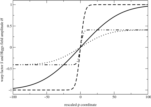
FIG. 1.: The rescaled Higgs field amplitude $H$ (full line for $\beta=0.01$ and dashed line for $\beta=0.1$) and warp factor derivative $S$ (dotted line for $\beta=0.01$ and dot-dashed line for $\beta=0.1$) as functions of the rescaled extra dimension coordinate $\varrho$.

Eqs. (12 -13) have been solved numerically with the relevant boundary conditions. The field profiles are depicted on Fig. 1 for two arbitrary values of the parameter $\beta$.

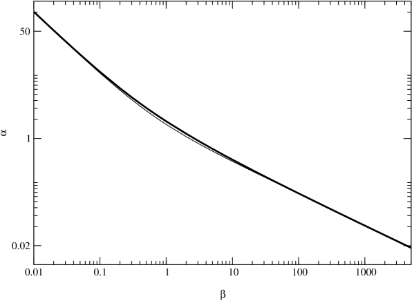
FIG. 2.: Relation between the dimensionless constants $\alpha$ and $\beta$. The thick curve represent the result of the numerical integration, while the (hardly distinguishable) thin curve is the best analytical fit.

The relation between the parameters $\alpha$ and $\beta$ such that the metric is regular at the brane location is depicted on Fig. 2. As can be seen on the figure, it consists essentially in two power laws. For small values of $\beta$, one finds roughly $\alpha\sim 1/\beta$, which becomes exact in the limit $\beta\to 0$, while for large values of $\beta$, one gets $\alpha\sim{4\over 3}\beta^{-1/2}$, which is, again, exact in the limit $\beta\to\infty$. We were able to find the best fit

$$\alpha^{2}={1\over\beta}\left[{1\over\beta}+\left({4\over 3}\right)^{2}\right],$$ (15)

which, as can be seen on the figure, is almost exact everywhere. This translates into the relation

$$|\Lambda|={1\over 9}\lambda\eta\left(\sqrt{1+\left({9\kappa_{5}^{2}\eta^{2}\over 8}\right)^{2}}-1\right)$$ (16)

between the 5 dimensional cosmological constant and the microscopic parameters, which corresponds to the usual relations between brane and bulk cosmological constants.

III Localization of fermions on the wall

This section is devoted to the description of the Dirac equation in five dimensions with the domain wall configuration obtained in the previous section.

The minimal representation of spinors in five dimensions can be chosen to be four dimensional [16]. The five dimensional Clifford algebra can then be constructed from the usual four dimensional one by adding the $\gamma_{5}$ matrix to close the algebra. If $\gamma^{\mu}$ design the usual four dimensional Dirac matrices in Minkowski space in the chiral representation, the Dirac matrices in five dimensional Minkowski space, $\Gamma^{A}$, are

$$\Gamma^{\mu}=\gamma^{\mu},\qquad\Gamma^{4}=-i\gamma_{5}$$ (17)

and they satisfied the usual Clifford algebra

$$\{\Gamma^{A},\Gamma^{B}\}=2\eta^{AB}$$ (18)

where $\eta^{AB}$ stands for the five dimensional Minkowski metric. Since in this representation the Dirac matrices satisfy

$$\Gamma^{5}=i\Gamma^{0}\dots\Gamma^{4}=\mathrm{Id}$$ (19)

the five dimensional spinors have neither Weyl nor Majorana represention. It follows that the Dirac Lagrangian in five dimension for fermions coupled to the Higgs domain wall is necessary of the form

$${\mathcal{L}}_{\psi}=\sqrt{g}\left(i\overline{\Psi}\Gamma^{A}{\cal D}_{A}\Psi-g_{{}_{\rm F}}{\overline{\Psi}}\Phi\Psi\right)=\sqrt{g}\,{\overline{\Psi}}\left[i\hbox{e}^{\sigma(y)}\Gamma^{\mu}{\cal D}_{\mu}+i\Gamma^{4}\partial_{y}-g_{{}_{\rm F}}\Phi\right]\Psi$$ (20)

where the Lorentz covariant derivative with spin connection is [17]

$${\cal D}_{\mu}\equiv\partial_{\mu}-\frac{1}{2}\sigma^{\prime}(y)\hbox{e}^{-\sigma(y)}\Gamma_{\mu}\Gamma^{4}.$$ (21)

We emphasize that the sign of the coupling $g_{{}_{\rm F}}$ of the spinor $\Psi$ to the Higgs field is arbitrary and represents a coupling either to kink or to anti-kink domain wall. For definiteness, we shall consider in what follows only the case of a kink coupling, and thus assume without lack of generality that $g_{{}_{\rm F}}>0$.

The variation of the Lagrangian (20) leads to the equation of motion of the spinor field, namely the Dirac equation in five dimensional anti-de Sitter space for a fermionic field coupled to a Higgs field,

$$\left[i\Gamma^{4}\left(\partial_{y}-2\sigma^{\prime}(y)\right)+i\hbox{e}^{\sigma(y)}\Gamma^{\mu}\partial_{\mu}-g_{{}_{\rm F}}\Phi\right]\Psi=0.$$ (22)

This equation involves the matrix $\gamma_{5}$ (through $\Gamma_{4}$) and it is thus convenient to split the four dimensional right- and left-handed components of the five dimensional spinor and to separate the variables as

$$\Psi(x^{\mu},y)=\left[\frac{1+\gamma_{5}}{2}{\mathcal{U}}_{\rm R}(y)+\frac{1-\gamma_{5}}{2}{\mathcal{U}}_{\rm L}(y)\right]\psi(x^{\mu}),$$ (23)

where $\psi(x^{\mu})$ is a four dimensional Dirac spinor, while ${\mathcal{U}}_{\rm R}(y)$ and ${\mathcal{U}}_{\rm L}(y)$ are yet-underdetermined functions of $y$. In what follows, we want the five dimensional Dirac equation to yield an effective four dimensional massive Dirac equation, with an effective mass $m$ (energy eigenvalue of the bound state). Such a requirement implies that

$$i\gamma^{\mu}\partial_{\mu}\psi=m\psi,$$ (24)

or, equivalently, in terms of the right- and left- handed components

$$i\gamma^{\mu}\partial_{\mu}\psi_{\rm R}=m\psi_{\rm L},\qquad i\gamma^{\mu}\partial_{\mu}\psi_{\rm L}=m\psi_{\rm R},$$ (25)

where the right- and left-handed components of the four dimensional spinor are defined as

$$\psi_{\rm R}\equiv\frac{1+\gamma_{5}}{2}\psi\qquad\textrm{and}\qquad\psi_{\rm L}\equiv\frac{1-\gamma_{5}}{2}\psi.$$ (26)

Contrary to the case studied in Ref. [10], the mass $m$ is not an arbitrary parameter and will be determined later.

Choosing $\psi_{\rm R}$ and $\psi_{\rm L}$ as the independent variables instead of $\Psi$ and $\overline{\Psi}$, and inserting equation (25) into the equation of motion (22) while using the splitting ansatz (23) yields the differential system for the two functions ${\mathcal{U}}_{{\rm R}/{\rm L}}(y)$,

$$\left[\partial_{y}-2\sigma^{\prime}(y)-g_{{}_{\rm F}}\Phi\right]{\mathcal{U}}_{\rm R}(y) = -m{\rm e}^{\sigma(y)}{\mathcal{U}}_{\rm L}(y),$$ (27)

$$\left[\partial_{y}-2\sigma^{\prime}(y)+g_{{}_{\rm F}}\Phi\right]{\mathcal{U}}_{\rm L}(y) = m{\rm e}^{\sigma(y)}{\mathcal{U}}_{\rm R}(y).$$ (28)

To simplify the notations, it is convenient to introduce the dimensionless rescaled bulk components of the fermions

$$\widetilde{\mathcal{U}}(\varrho)\equiv{\rm e}^{-\frac{3}{2}\sigma(\varrho)}\frac{{\mathcal{U}}(\varrho)}{|\Lambda|^{1/4}},$$ (29)

in terms of which the system (27-28) takes the form

$$\left(\partial_{\varrho}-\left[\gamma_{{}_{\rm F}}H+\frac{1}{2}S\right]\right)\,\widetilde{\mathcal{U}}_{\rm R} = -\mu\,{\rm e}^{\sigma}\widetilde{\mathcal{U}}_{\rm L},$$ (30)

$$\left(\partial_{\varrho}+\left[\gamma_{{}_{\rm F}}H-\frac{1}{2}S\right]\right)\,\widetilde{\mathcal{U}}_{\rm L} = \mu\,{\rm e}^{\sigma}\widetilde{\mathcal{U}}_{\rm R},$$ (31)

with the dimensionless rescaled mass and coupling constant

$$\mu\equiv\frac{m}{\sqrt{|\Lambda|}}\quad\textrm{and}\quad\gamma_{{}_{\rm F}}\equiv\frac{g_{{}_{\rm F}}\eta}{\sqrt{|\Lambda|}}.$$ (32)

Let us first concentrate on the special case $\mu=0$. The system (30-31) then consists in two decoupled differential equations and the zero mode states [18] are recovered. Asymptotically, these functions behave as

$$\widetilde{\mathcal{U}}_{\rm R}(\varrho\rightarrow\pm\infty) \sim {\rm e}^{\left(\gamma_{{}_{\rm F}}+\frac{1}{2\sqrt{6}}\right)|\varrho|},$$ (33)

$$\widetilde{\mathcal{U}}_{\rm L}(\varrho\rightarrow\pm\infty) \sim {\rm e}^{-\left(\gamma_{{}_{\rm F}}-\frac{1}{2\sqrt{6}}\right)|\varrho|}.$$ (34)

Thus, only the left-handed solution $\widetilde{\mathcal{U}}_{\rm L}$ may remain bounded [7, 9], and yet provided

$$\gamma_{{}_{\rm F}}>\frac{1}{2\sqrt{6}}.$$ (35)

Indeed, the right-handed zero modes could have been obtained by considering the coupling of fermions to the anti-kink Higgs profile. We thus recover the well-known fact that massless fermions must be single-handed in a brane model, contrary to the ordinary four dimensional field theory in which they simply can.

Let us now focus on the more interesting massive case for which $\mu\not=0$. Then the system (30-31) can be decoupled by eliminating $\widetilde{\mathcal{U}}_{\rm R}$ say. For that purpose, we differentiate (31) with respect to $\varrho$ and express $\partial_{\varrho}\widetilde{\mathcal{U}}_{\rm R}$ using equation (30) and $\widetilde{\mathcal{U}}_{\rm R}$ using equation (31) again to get

$$\left[\partial^{2}_{\varrho}-2S\,\partial_{\varrho}+\left(\mu^{2}{\rm e}^{2\sigma}+\frac{3}{4}S^{2}-\gamma_{{}_{\rm F}}^{2}H^{2}-\gamma_{{}_{\rm F}}SH-\frac{1}{2}\partial_{\varrho}S+\gamma_{{}_{\rm F}}\partial_{\varrho}H\right)\right]\widetilde{\mathcal{U}}_{\rm L}=0,$$ (36)

$$\widetilde{\mathcal{U}}_{\rm R}=\frac{{\rm e}^{-\sigma}}{\mu}\left[\partial_{\varrho}+\left(\gamma_{{}_{\rm F}}H-\frac{1}{2}S\right)\right]\widetilde{\mathcal{U}}_{\rm L}.$$ (37)

This system is strictly equivalent to the initial system (30-31) since differentiating Eq. (37) and then using Eq. (36) gives back Eq. (30). It is thus important to keep both equations. Note that the integration of the first equation (36) will require two initial conditions but that $\widetilde{\mathcal{U}}_{\rm R}$ will then be completely determined and thus requires no extra constant of integration. As a consequence, it is sufficient to solve the second order equation (36) for $\widetilde{\mathcal{U}}_{\rm L}$ in order to fully determine the left- and right-handed bulk fermion profiles.

Eq. (36) can be recast into a Schrödinger-like second order differential equation

$$\partial^{2}_{\varrho}\,\widehat{\mathcal{U}}_{\rm L}+\omega^{2}(\varrho)\,\widehat{\mathcal{U}}_{\rm L}=0,$$ (38)

where the function $\omega$ is defined by

$$\omega^{2}(\varrho)\equiv\mu^{2}{\rm e}^{2\sigma(\varrho)}+\partial_{\varrho}\left(\gamma_{{}_{\rm F}}H+\frac{1}{2}S\right)-\left(\gamma_{{}_{\rm F}}H+\frac{1}{2}S\right)^{2}$$ (39)

with the new function

$$\widehat{\mathcal{U}}(\varrho)\equiv{\rm e}^{-\sigma(\varrho)}\widetilde{\mathcal{U}}(\varrho).$$ (40)

Our aim will now be to find the zero modes of this new equation; as previously discussed, they will be equivalent to the massive bound states we are looking for on the brane.

In order for the fermions to be confined on the brane, the minimum of $\omega^{2}$ needs to be negative to imply an exponential decrease of $\widehat{\mathcal{U}}_{\rm L}$ in the bulk. This is essentially equivalent to the condition (35) that was obtained for the case of zero modes. We shall assume henceforth that this condition also holds for massive modes, i.e., that the value of $\gamma_{{}_{\rm F}}$ necessary to bind massive fermions on the brane is at least that to bind massless ones. Indeed, Eq. (39) shows that the minimum of $\omega^{2}$ can only be negative for large values of the parameter $\gamma_{{}_{\rm F}}$. However, since the first term of (39) increases exponentially at large distance from the brane, then, if $\mu\not=0$, $\omega^{2}$ will necessarily become positive. This will yield asymptotic radiative behaviors of the spinor bulk components. Physically, it can be interpreted as a tunneling of the fermions from the brane to the bulk [10]. On the other hand, on the brane, the Higgs field $H$ and the derivative of the warp factor $S$ vanish, so that $\omega^{2}(0)$ is positive. As a result, the fermions can freely propagate in a tiny region around the brane, but certainly only for particular values of $\omega^{2}$ (and thus of $\mu$) satisfying the boundary conditions with the surrounding exponential decreasing regions. The effective potential $V_{{}_{\rm eff}}=-\omega^{2}$, depicted in Fig. 3, exhibits a local minimum on the brane and minima at infinity. The modes trapped on the brane are thus expected to have discrete masses $\mu$ on the brane and non-zero probability of tunneling into the bulk.

FIG. 3.: The effective potential $V_{{}_{\rm eff}}=-\omega^{2}$ felt by $\widehat{\mathcal{U}}_{\rm L}$. We chose the parameters $\gamma_{{}_{\rm F}}=100$ and $\mu=0.5\gamma_{{}_{\rm F}}$ (an illustrative value, not necessarily leading to a bound state) in the Higgs and gravity background similar to those of Fig. 1, and we have assumed, for definiteness, the values $\alpha=1.63$, $\beta=1.23$. The fermions are trapped on the brane where $V_{{}_{\rm eff}}$ is negative and have a non-zero probability of tunneling into the bulk due to combined effects of Higgs and gravity which produce a finite potential barrier.

IV Analytic estimate of the mass spectrum and of the tunneling rate

Since the Higgs and warp factor profiles are not known analytically, it is a priori impossible to solve Eq. (38) analytically. Nevertheless, since the fermions are expected to be trapped in a neighborhood of the brane, we can look for series solutions in $\varrho$.

In § IV A, we give an approximation of the effective potential $V_{{}_{\rm eff}}$ which will then be used to determine the bound states and the mass spectrum in § IV B. We end this section by determining in § IV C the tunneling rate in this approximation. The validity of this approach is difficult to assess and it will be justified a posteriori on the ground of a full numerical integration of the system in the following section. In the whole section, it is assumed that $\mu>0$.

A Approximation of the effective potential

In a neighborhood of the brane we can expand the Higgs and warp factor profiles as

$$H(\varrho) = H_{1}\varrho+H_{3}\varrho^{3}+{\mathcal{O}}(\varrho^{4}),$$ (41)

$$S(\varrho) = S_{1}\varrho+S_{3}\varrho^{3}+{\mathcal{O}}(\varrho^{4}),$$ (42)

where both the constant and quadratic terms vanish for symmetry reasons. To simplify the analysis, we shall make use of the equations of motion in the form

$$\dot{S}={2\over 3}F(S,H),$$ (43)

and

$$\dot{H}=\pm\sqrt{{2\over\alpha}F(S,H)},$$ (44)

where the function $F(S,H)$ is defined as

$$F(S,H)\equiv 6S^{2}+\alpha\beta(H^{2}-1)^{2}-1,$$ (45)

(recall that $\Lambda<0$).

Plugging the expansions (41) and (42) into Eqs. (43) and (44), it follows that the function $F(S,H)$ can be expanded up to third order as

$$F(S,H)\sim\alpha\beta-1+\left(6S_{1}^{2}-2\alpha\beta H_{1}^{2}\right)\varrho^{2}+{\mathcal{O}}(\varrho^{4}).$$ (46)

Inserting this expression back into the equations of motion yields the three coefficients

$$S_{1} = \frac{\alpha}{3}H_{1}^{2},$$ (47)

$$S_{3} = \frac{4}{9}\alpha H_{1}^{2}\left[\frac{\alpha}{3}H_{1}^{2}-\beta\right],$$ (48)

$$H_{3} = \frac{2}{3}H_{1}\left[\frac{\alpha}{3}H_{1}^{2}-\beta\right]$$ (49)

in terms of the coefficient $H_{1}$

$$H_{1}\equiv\left.\partial_{\varrho}H\right|_{\varrho=0}=\sqrt{\frac{2}{\alpha}(\alpha\beta-1)}.$$ (50)

Then, the frequency $\omega^{2}$ can be expanded as an harmonic oscillator potential

$$\omega^{2}(\varrho)=\omega_{\rm b}^{2}(\varrho)+{\mathcal{O}}(\varrho^{4})\qquad\hbox{with}\qquad\omega^{2}_{\rm b}(\varrho)\equiv\omega_{0}^{2}-\Omega\,\varrho^{2}$$ (51)

where $\omega_{0}^{2}$ and $\Omega$ are given by

$$\omega_{0}^{2} \equiv \mu^{2}+\gamma_{{}_{\rm F}}H_{1}\left(1+\frac{\alpha}{6\gamma_{{}_{\rm F}}}H_{1}\right)$$ (52)

$$\Omega \equiv H_{1}\gamma_{{}_{\rm F}}^{2}\left[H_{1}+\frac{2}{\gamma_{{}_{\rm F}}}\left(\beta-\frac{\alpha}{6}H_{1}^{2}\right)+\frac{\alpha}{3\gamma_{{}_{\rm F}}^{2}}H_{1}\left(2\beta-\mu^{2}-\frac{7\alpha}{12}H_{1}^{2}\right)\right].$$ (53)

The function $\omega^{2}$ is well approximated by $\omega_{\rm b}^{2}$ only near the brane and the expansion (51) is no longer valid at large distance where the exponential term dominates [see Eq. (39)]. Once the fixed asymptotic values of the Higgs and warp factor are reached, the frequency (39) behaves as

$$\omega^{2}\sim\omega^{2}_{\infty}(\varrho)\qquad\hbox{with}\qquad\omega^{2}_{\infty}=\mu^{2}{\rm e}^{2|\varrho|/\sqrt{6}}-\left(\gamma_{{}_{\rm F}}+\frac{1}{2\sqrt{6}}\right)^{2}.$$ (54)

The analytical estimate of the function $\omega^{2}$ is thus obtained by matching the two limiting asymptotic behaviors (51) and (54), respectively $\omega_{\rm b}^{2}$ closes to the brane and $\omega^{2}_{\infty}$ far from it, as

$$\omega^{2}(\rho)=\left\{\begin{array}[]{cc}\omega_{\rm b}^{2}&|\rho|<\rho_{{}_{\rm m}}\\ \omega_{\infty}^{2}&|\rho|>\rho_{{}_{\rm m}}\end{array}\right.$$ (55)

The dimensionless matching distance $\varrho_{{}_{\rm m}}$ has to be solution of

$$\omega^{2}_{{}_{\rm b}}(\varrho_{{}_{\rm m}})=\omega^{2}_{\infty}(\varrho_{{}_{\rm m}}),$$ (56)

in order to get a continuous function. Note that, because of the symmetry on both sides of the wall, we can assume $\varrho_{{}_{\rm m}}>0$ without lack of generality. For large values of $\gamma_{{}_{\rm F}}$, and using Eq. (53), we get

$$\sqrt{\Omega}\sim\gamma_{{}_{\rm F}}H_{1},$$ (57)

leading to

$$\varrho_{{}_{\rm m}}\sim\frac{1}{H_{1}}.$$ (58)

As it turns out, the faster the asymptotic solution is reached, the better the approximation works. This is the case in particular for $H_{1}>1$,

The exact (numerically integrated) effective potential and its approximation are compared in Fig. 4. The global shapes are effectively the same, and in spite of uncertainties at intermediate regions due to this crude approximation, it is reasonable to expect the same fermion physical behaviors in both potentials. Note that for (cosmologically favored) higher value of $\alpha\beta$, the Higgs field and the warp factor reach more rapidly their asymptotic values leading thus to a better agreement between the two potentials, as can be seen on Fig. 4.

B Determination of the bound states

Given the approximate frequency (55), the equation of motion for the left-handed bulk spinor component $\widehat{\mathcal{U}}_{\rm L}$ reduces to

$$\varrho>\varrho_{{}_{\rm m}}: \left[\partial_{\varrho}^{2}+\mu^{2}{\rm e}^{2|\varrho|/\sqrt{6}}-\left(\gamma_{{}_{\rm F}}+\frac{1}{2\sqrt{6}}\right)^{2}\right]\widehat{\mathcal{U}}_{\rm L}=0,$$ (59)

$$\varrho<\varrho_{{}_{\rm m}}: \left[\partial_{\varrho}^{2}+\omega_{0}^{2}-\Omega\varrho^{2}\right]\widehat{\mathcal{U}}_{\rm L}=0,$$ (60)

with the requirement that $\widehat{\mathcal{U}}_{\rm L}$ and its derivative are continuous at $\varrho_{{}_{\rm m}}$. Note also that we consider only the case $\varrho>0$, physics on both sides of the brane being completely symmetric under the transformation $\varrho\to-\varrho$. Let us consider the solutions in each region separately.

FIG. 4.: The effective potential $V_{{}_{\rm eff}}=-\omega^{2}$ and the approximate analytic effective potential (dashed curve) obtained from the matching of its two asymptotic expansions near the brane and at infinity. On the left panel, the parameters are the same as on Fig. 3, i.e., $\gamma_{{}_{\rm F}}=100$ and $\mu=0.5\gamma_{{}_{\rm F}}$. As the asymptotic solution is not reached very close to the brane, the approximation is rather poor and the two solutions are not in good agreement at intermediate regions. On the right panel, we use the new parameter values $\gamma_{{}_{\rm F}}=100$ and $\mu=0.6\gamma_{{}_{\rm F}}$, obtained for $\alpha=0.1865$ and $\beta=53.62$, a much better approximation is obtained around the potential barrier provided the Higgs field and warp factor reach their vacuum value rapidely, i.e., for larger value of $\alpha\beta$. As on Fig. 3, the parameters are chosen to illustrate the point and do not necessarily correspond to existing bound states.

• $\varrho>\varrho_{{}_{\rm m}}$: we introduce the new variable

  $$z\equiv\sqrt{6}\mu{\rm e}^{|\varrho|/\sqrt{6}},$$ (61)

  in terms of which Eq. (59) reduces to a standard Bessel differential equation

  $$\left[\frac{{\rm d}^{2}}{{\rm d}z^{2}}+\frac{1}{z}\frac{{\rm d}}{{\rm d}z}+\left(1-\frac{\ell^{2}}{z^{2}}\right)\right]\,\widehat{\mathcal{U}}_{\rm L}=0,$$ (62)

  the order of which being given by

  $$\ell=\sqrt{6}\gamma_{{}_{\rm F}}+\frac{1}{2}.$$ (63)

  Since $\omega^{2}$ is positive at infinity, the asymptotic form of the solution is necessary radiative, as was already pointed out in the previous section. The most general solution of the Bessel equation (62) is a linear superposition of Hankel functions. Since we are interested only in ingoing waves in order to study a tunneling process, the most general solution takes the form

  $$\widehat{\mathcal{U}}_{\rm L}(z)=B\,H^{(1)}_{\ell}(z),$$ (64)

  where $H^{(1)}_{\ell}(z)$ is the Hankel function of the first kind, propagating towards the brane at infinity [19]

  $$H^{(1)}_{\ell}(z\rightarrow\infty)\sim\sqrt{\frac{2}{\pi z}}\,{\rm e}^{i(z-\ell\pi/2-\pi/4)}.$$ (65)

  and $B$ is an arbitrary complex constant.

• $\varrho<\varrho_{{}_{\rm m}}$: performing operations similar to those of the previous case, we cast Eq. (60) on the form

  $$\left[\frac{{\rm d}^{2}}{{\rm d}x^{2}}-\left(\frac{1}{4}x^{2}+a\right)\right]\widehat{\mathcal{U}}_{\rm L}=0,$$ (66)

  in which we have introduced the new variable and parameter

  $$x\equiv\left(4\Omega\right)^{\frac{1}{4}}\varrho,\ \ \ \ \ a\equiv-\frac{\omega_{0}^{2}}{2\sqrt{\Omega}}.$$ (67)

  The general solutions of Eq. (66) are the parabolic cylinder functions, namely $U(a,x)$ and $V(a,x)$, of which $\widehat{\mathcal{U}}_{\rm L}(x)$ can be expressed as linear superpositions. In the limit $x\gg|a|$, these solutions scale as [20]

  $$U(a,x)\sim{\rm e}^{-\frac{1}{4}x^{2}}x^{-a-\frac{1}{2}}, V(a,x)\sim\sqrt{\frac{2}{\pi}}\,{\rm e}^{\frac{1}{4}x^{2}}x^{a-\frac{1}{2}}.$$ and (68)

  Since we are interested in confined fermion states on the brane, only the exponentially decreasing function is relevant, so that the general solution near the brane reads

  $$\widehat{\mathcal{U}}_{\rm L}(x)=A\,U(a,x),$$ (69)

  where $A$ is a complex integration constant.

The general solution $\widehat{\mathcal{U}}_{\rm L}(\varrho)$ for all $\varrho$ is obtained by matching the two different solutions at $\varrho=\varrho_{{}_{\rm m}}$. Since $\varrho_{{}_{\rm m}}$ corresponds to the maximum positive value of the effective potential [see Fig. 4], it is reasonable to consider that the Hankel function at that point can be expanded around small values of their argument with respect to their order [19], i.e.,

$$H^{(1)}_{\ell}(z_{{}_{\rm m}})\sim-\frac{2^{\ell}}{\pi}\Gamma(\ell)z_{{}_{\rm m}}^{-\ell},$$ (70)

while the parabolic cylinder functions can be taken in their large argument asymptotic limit (68). This is the same kind of approximation as that made to derive the effective potential. Physically, the initial conditions on the brane, i.e., $\widehat{\mathcal{U}}_{\rm L}(0)$ and $\partial_{\varrho}\widehat{\mathcal{U}}_{\rm L}|_{0}$, are chosen in such a way that the asymptotic exponentially growing function $V(a,x)$ contribution is everywhere negligible. Once these initial conditions are fixed, they fully determine the solution on the other side of the brane, i.e., for $x<0$. The asymptotic expansion (68) can be analytically extended to $-|x|=|x|{\rm e}^{i\pi}$ and yields [21]

$$U(a,-|x|)\sim{\rm e}^{-\frac{1}{4}|x|^{2}}|x|^{-a-\frac{1}{2}}{\rm e}^{-i\pi\left(a+\frac{1}{2}\right)}.$$ (71)

Thus, once $\widehat{\mathcal{U}}_{\rm L}(0)$ and $\partial_{\varrho}\widehat{\mathcal{U}}_{\rm L}|_{0}$ are fixed, the matchings between $H^{(1)}_{\ell}(z_{{}_{\rm m}})$ and $U(a,-|x_{{}_{\rm m}}|)$ on one side, and $U(a,|x_{{}_{\rm m}}|)$ on the other side fully determine the bulk component $\widehat{\mathcal{U}}_{\rm L}$ for all $\varrho$.

The last constraint comes from Eq. (37) determining the right-handed spinor bulk function. It is well defined if and only if both $\widehat{\mathcal{U}}_{\rm L}$ and $\partial_{\varrho}\widehat{\mathcal{U}}_{\rm L}$ are not singular. In fact, the derivative of the parabolic cylinder function $U(a,x)$ is generally discontinuous at $x=0$. With the help of the Wronskian of $U(a,x)$ and $U(a,-x)$ [20]

$$U(a,x)\frac{{\rm d}U(a,-x)}{{\rm d}x}-U(a,-x)\frac{{\rm d}U(a,x)}{{\rm d}x}=\frac{2\pi}{\Gamma\left(\frac{1}{2}+a\right)},$$ (72)

we can construct the derivative discontinuity at $x=0$. This is

$$\frac{{\rm d}U(a,0^{-})}{{\rm d}x}-\frac{{\rm d}U(a,0^{+})}{{\rm d}x}=2^{\frac{a}{2}+\frac{3}{4}}\frac{\Gamma\left(\frac{3}{4}+\frac{a}{2}\right)}{\Gamma\left(\frac{1}{2}+a\right)},$$ (73)

where we have used the particular value [20]

$$U(a,0)=\frac{\sqrt{\pi}}{2^{\frac{a}{2}+\frac{1}{4}}\Gamma\left(\frac{3}{4}+\frac{a}{2}\right)}.$$ (74)

Imposing that the derivative of $\widehat{\mathcal{U}}_{\rm L}$ is continuous at $x=0$ results in imposing that the jump (73) vanishes. This is the case if and only if $a$ is solution of

$$\frac{\Gamma\left(\frac{3}{4}+\frac{a}{2}\right)}{\Gamma\left(\frac{1}{2}+a\right)}=0.$$ (75)

Since $\Gamma$ is singular for negative integer arguments, this condition is satisfied only for

$$-a-\frac{1}{2}=2n,$$ (76)

where $n$ is a positive integer. Note that $-a-1/2$ cannot be odd since then the numerator of the Wronskian (75) will also be singular resulting in a finite derivative jump at $x=0$. The condition (76) shows that the trapped fermions on the brane have necessarily discrete masses $\mu_{n}$ which read, using the values of the parameters (52), (53) and (67),

$$\mu^{2}_{n} = \gamma_{{}_{\rm F}}H_{1}\left[(4n+1)\sqrt{1+\frac{6\beta}{3\gamma_{{}_{\rm F}}H_{1}}+\frac{24\alpha\beta+\alpha^{2}H_{1}^{2}\left[(4n+1)^{2}-5\right]}{36\gamma_{{}_{\rm F}}^{2}}}\right.-\left.\left(1+\frac{\alpha H_{1}}{6\gamma_{{}_{\rm F}}}\left[(4n+1)^{2}+1\right]\right)\right].$$ (77)

This mass spectrum is valid for $n>0$ since our derivation assumed that $\mu>0$. In the limiting case where $\gamma_{{}_{\rm F}}\gg 1$, it reduces to the much simpler form for the lowest masses

$$\mu_{n}\sim 2\sqrt{n}\sqrt{\gamma_{{}_{\rm F}}H_{1}}.$$ (78)

On the other hand, $\mu^{2}$ cannot reach very large values since it is necessary to have a potential barrier in order to have bound states. From the expression of the effective potential (54), the barrier is found to disappear when

$$\omega_{\infty}^{2}(\varrho_{{}_{\rm m}},\mu_{\max})\sim 0.$$ (79)

Again in the limit where $\gamma_{{}_{\rm F}}\gg 1$, using the value (58) of $\varrho_{{}_{\rm m}}$, one gets the maximum accessible reduced mass $\mu_{\max}$ for $\mu$ as

$$\mu_{\max}\sim\gamma_{{}_{\rm F}}{\rm e}^{-1/\sqrt{6}H_{1}}.$$ (80)

The maximum number of distinct massive states trapped on the brane can thus be estimated to be

$$n_{\max}\sim{\mathrm{Int}}\left[\gamma_{{}_{\rm F}}\frac{1}{4H_{1}}{\rm e}^{-2/\sqrt{6}H_{1}}\right].$$ (81)

For the parameters chosen in Fig. 3, one obtains $\mu_{\max}\sim 0.68\gamma_{{}_{\rm F}}$ and there are $n_{\max}=11$ massive modes trapped on the brane.

C Fermion tunneling rate

Since the effective potential becomes negative at infinity, the massive modes trapped on the brane are subject only to a finite potential barrier. They are in a metastable state and can tunnel from the brane to the bulk. In this section we use our previous analytic solution to estimate the tunneling rate. Would this rate be too high, one would observe an effective violation of energy-momentum conservation on the brane, i.e., in four dimension, thereby contradicting observation.

Our starting point is the analytic solution for the left-handed bulk function that was derived in the previous section

$$\varrho<\varrho_{{}_{\rm m}}: \widehat{\mathcal{U}}_{\rm L}(\varrho)=A\,U\left(a,\sqrt{2}\Omega^{1/4}\varrho\right),$$ (82)

$$\varrho>\varrho_{{}_{\rm m}}: \widehat{\mathcal{U}}_{\rm L}(\varrho)=B\,H^{(1)}_{\ell}\left(\sqrt{6}\mu{\rm e}^{|\varrho|/\sqrt{6}}\right).$$ (83)

The transmission factor can easily be derived from the matching conditions of the left-handed bulk fermion component at $\varrho=\varrho_{{}_{\rm m}}$. First of all, $\widehat{\mathcal{U}}_{\rm L}$ has to be continuous. Using the expansions (68) and (70) and the value (76) of the parameter $a$, permits to find the relation

$$A\,{\rm e}^{-\frac{1}{2}\sqrt{\Omega}\varrho_{{}_{\rm m}}^{2}}\left(2\sqrt{\Omega}\right)^{n}\varrho_{{}_{\rm m}}^{2n}=-\frac{i}{\pi}B\,\Gamma(\ell)\left(\sqrt{\frac{3}{2}}\mu_{n}\right)^{-\ell}{\rm e}^{-\ell\varrho_{{}_{\rm m}}/\sqrt{6}}$$ (84)

between the coefficients $A$ and $B$. Making use of the expression (58) for $\varrho_{{}_{\rm m}}$ yields

$$\frac{B}{A}=\frac{i\pi}{\Gamma(\ell)}\left(\sqrt{\frac{3}{2}}\mu_{n}\right)^{\ell}\left(\frac{\ell^{2}}{3\sqrt{\Omega}}\right)^{n}\exp{\left[\frac{\ell^{2}}{12\sqrt{\Omega}}\right]}.$$ (85)

Assuming, as above, that $\gamma_{{}_{\rm F}}\gg 1$ (so that $\ell\gg 1$) we can expand $\Gamma(\ell)$ as

$$\Gamma(\ell)\sim\ell^{\ell-1/2}{\rm e}^{-\ell}\sqrt{2\pi},$$ (86)

so that, using expressions (57), (58) and (63) respectively of $\Omega$, $\varrho_{{}_{\rm m}}$, and $\ell$, we get that $B/A$ is approximated by

$$\frac{B}{A}\sim i\sqrt{\frac{\pi}{2}}\left(\frac{2}{H_{1}}\right)^{n}6^{1/4}\gamma_{{}_{\rm F}}^{n+1/2}\exp{\left[-\sqrt{6}\gamma_{{}_{\rm F}}\left(\ln{\frac{2\mu_{\max}}{\mu}}-1+\frac{1}{2\sqrt{6}H_{1}}\right)\right]}.$$ (87)

The transmission coefficient from the brane to the bulk associated with $\widehat{\mathcal{U}}_{\rm L}$ can thus be defined by

$$\widehat{\mathcal{T}}\equiv\frac{\widehat{\mathcal{U}}_{\rm L}(\ell)}{\widehat{\mathcal{U}}_{\rm L}(0)},$$ (88)

with $\widehat{\mathcal{U}}_{\rm L}(\ell)=BH_{\ell}^{(1)}(\ell)$, is evaluated at the turning point $\varrho=\ell$ where the spinor bulk component begins to propagate freely. Using the behaviour (74) of the function at the origin, the ratio (87) and the properties [19] of the Hankel function

$$H^{(1)}_{\ell}(\ell)=\left(\frac{4}{3}\right)^{2/3}\frac{{\rm e}^{-i\pi/3}}{\Gamma(2/3)}\,\ell^{-1/3},$$ (89)

the transmission coefficient (88) reduces to

$$\widehat{\mathcal{T}} \sim \frac{2^{4/3}\Gamma(1/2-n)}{3^{7/12}\Gamma(2/3)}{\rm e}^{i\pi/6}H_{1}^{-n}\gamma_{{}_{\rm F}}^{n+1/6}\exp{\left[-\sqrt{6}\gamma_{{}_{\rm F}}\left(\ln{\frac{2\mu_{\max}}{\mu}}-1+\frac{1}{2\sqrt{6}H_{1}}\right)\right]}.$$ (90)

It follows, using the definition (40), that the probability for a trapped particle on the brane to tunnel to the bulk is given by

$${\mathcal{P}}\equiv|\widetilde{\mathcal{T}}|^{2}={\rm e}^{2\ell/\sqrt{6}}\,|\widehat{\mathcal{T}}|^{2}.$$ (91)

The characteristic time for a fermionic mode trapped on the brane can be roughly estimated by

$$\tau_{{}_{\rm b}}\sim y_{{}_{\rm b}}=\frac{\varrho_{{}_{\rm b}}}{\sqrt{|\Lambda|}},$$ (92)

where $y_{{}_{\rm b}}$ represents the typical length, in the fifth dimension, felt by a particle on the brane. As can be seen on Fig. 5, the spinor bulk components are exponentially damped as soon as the effective potential becomes positive. Thus $\varrho_{{}_{\rm b}}$ can be estimated by the solution of $\omega_{{}_{\rm b}}^{2}(\varrho_{{}_{\rm b}})=0$ so that, keeping in mind that $\mu<\gamma_{{}_{\rm F}}$,

$${\varrho_{{}_{\rm b}}}^{-1}\sim\sqrt{H_{1}\gamma_{{}_{\rm F}}}.$$ (93)

The life-time $\tau_{n}$ of a fermionic bound state on the brane labelled by $n$

$$\tau_{n}=\frac{\tau_{{}_{\rm b}}}{{\mathcal{P}}}$$ (94)

can be estimated by

$$\tau_{n} \sim \frac{3^{7/6}\,\Gamma^{2}(2/3)}{2^{11/6}\,\Gamma^{2}(1/2-n)}H_{1}^{2n-1/2}\frac{\gamma_{{}_{\rm F}}^{-2n-5/6}}{\sqrt{|\Lambda|}}\,\exp{\left(2\sqrt{6}\gamma_{{}_{\rm F}}\left[\ln{\frac{2\mu_{\max}}{\mu_{n}}}-1-{1\over\sqrt{6}}+\frac{1}{2\sqrt{6}H_{1}}\right]\right)}.$$ (95)

We recall that, due to the approximations performed in the previous derivation, this estimate is valid only for $\mu\ll\mu_{\max}$. Nevertheless, the argument in the exponential amplifies the transition from bound states to tunneling ones for masses $\mu\sim\mu_{\max}$, as intuitively expected. An order of magnitude of the minimal coupling constant $\gamma_{{}_{\rm F}}$ leading to stable bound states can thus be estimated by requiring that the lowest massive state does not tunnel,

$$\mu_{1}<2\mu_{\max}\exp{\left(-1-{1\over\sqrt{6}}+\frac{1}{2\sqrt{6}H_{1}}\right)}.$$ (96)

Using the two values (78) and (80), this implies that

$$\gamma_{{}_{\rm F}}\gtrsim H_{1}\exp{\left(2+{2\over\sqrt{6}}+\frac{1}{\sqrt{6}H_{1}}\right)}.$$ (97)

As a numerical application, for the Higgs and gravity parameters used in Fig. 3, we get $\gamma_{{}_{\rm F}}\gtrsim 25$.

V Numerical investigation

Numerically, it is simpler and more convenient to solve the first order differential system (30-31). A Runge-Kutta integration method was used, on both sides of the brane. In order to suppress the exponential growth, we integrate from the turning point, $\varrho=\ell$, where the solution begins to propagate freely, toward the brane. In this way, we get only $U(a,x)$ near the brane. The radiative solution for $\varrho>\ell$, is simply obtained by integrating from the turning point toward infinity, with initial conditions determined by the matching with the exponential decreasing solution near the wall. The same method is used on the other side of the brane, but this time, by means of the last free parameter, we impose the continuity of one bulk spinor component on the brane ($\widetilde{\mathcal{U}}_{\rm L}$ say). Generally, the other bulk spinor component will be discontinuous at $\varrho=0$, as expected from the analytical study since $U^{\prime}(a,0)$ is generally discontinuous. The mass spectrum is thus obtained by requiring the continuity of $\widetilde{\mathcal{U}}_{\rm R}$ on the brane.

The bulk spinor components computed this scheme have been plotted for the first massive modes trapped on the brane in Fig. 6, for $\gamma_{{}_{\rm F}}=100$. The lowest mass is numerically found to be $\mu_{1}\sim 0.209\gamma_{{}_{\rm F}}$ and was estimated analytically, from (78), to be $\mu_{1}\sim 0.210\gamma_{{}_{\rm F}}$ leading to a precision of 0.5% for the analytical estimate. The second mass is numerically found to be $\mu_{2}\sim 0.291\gamma_{{}_{\rm F}}$, which has to be compared to its analytical estimate $\mu_{2}\sim 0.295\gamma_{{}_{\rm F}}$. Again, the precision of this estimate is of about 1%. As predicted from (81), there are $n_{\max}=11$ massive bound states the lightest masses of which are summed up in table I. On Fig. 5, we plot the last $n=11$ trapped mode; it has a tiny radiative component, as expected for a tunneling mode.

FIG. 5.: [Left] The right (dashed line) and left (solid line) bulk spinor components $\widetilde{\mathcal{U}}_{\rm R}$ and $\widetilde{\mathcal{U}}_{\rm L}$, as functions of the dimensionless distance $\varrho$ to the brane, for the heaviest massive state ($n=11$) and $\gamma_{{}_{\rm F}}=100$. [Right] Zoom near the turning point and transition to the radiative behaviour which takes place at a finite distance to the brane due to the tunneling of this mode from the brane to the bulk.

$n$	1	2	3	4	5	6	…	11
$\mu_{n}$ (numerical)	0.209	0.291	0.353	0.402	0.444	0.480	…	0.593
$\mu$ (estimates)	0.210	0.295	0.359	0.412	0.458	0.499	…	0.657
precision (%)	0.5	1.3	1.7	2.4	3	3.8	…	9.7

TABLE I.: Comparison of the numerical values and analytical estimates of the first six bound states reduced mass $\mu$, together with the heaviest mode, computed for $\gamma_{{}_{\rm F}}=100$.

In conclusion, the numerics confirm that the approximations of the previous section and our estimates are accurate up to 1%-10% (see table I).

FIG. 6.: The right (dashed curve) and left bulk spinor components, $\widetilde{\mathcal{U}}_{\rm R}$ and $\widetilde{\mathcal{U}}_{\rm L}$, as functions of the dimensionless distance $\varrho$ from the brane for the lightest massive bound states. They have been computed for $\gamma_{{}_{\rm F}}=100$ and in the Higgs and warp factor profiles obtained with parameter of Fig. 3. The numerical values of the corresponding reduced masses are reported on table I.

VI Discussion and conclusions

We shall now discuss the cosmological constraints existing on the kind of model we have been considering here. Most of these constraints come from brane models in which the wall structure is replaced by an infinitely thin four dimensional layer. As discussed in the previous sections, such an approximation is equivalent, within our framework, to asking that the combination $\alpha\beta$ be much larger than unity. In this limit, equivalent to the large $\beta$ limit since, from Eq. (15), $\alpha\beta\sim{4\over 3}\beta$, we can replace the stress-energy tensor (6) by the effective four dimensional surface distribution

$$T^{{}^{\rm eff}}_{\mu\nu}=T_{\infty}g_{\mu\nu}\delta(y),$$ (98)

whose isotropic tension $T_{\infty}$ is obtained by integration in the transverse direction to yield

$$T_{\infty}=\sqrt{|\Lambda|}\eta^{2}\int{\rm d}\varrho\,{\rm e}^{-6\sigma(\varrho)}\left[{1\over 2}\Phi^{\prime 2}+2V\right]\equiv\sqrt{|\Lambda|}\eta^{2}\xi(\beta)$$ (99)

where the function $\xi(\beta)$ can be expressed as

$$\xi=\int{\rm d}\varrho\,{\rm e}^{-6\sigma(\varrho)}\left[{6S^{2}-1\over\alpha}+2\beta(H^{2}-1)^{2}\right].$$ (100)

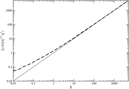
FIG. 7.: Effective four dimensional brane tension, in units of $\sqrt{|\Lambda|}\eta^{2}$, of the domain wall as a function of $\beta$ (dashed line). It is clear that in the thin brane limit, $\xi\simeq\beta$ (thin line).

Fig. 7 shows the variation of $\xi$ as a function of $\beta$. In the limit $\beta\gg 1$, it is clear that $\xi\simeq\beta$, so that the brane tension behaves as

$$T_{\infty}\simeq{\lambda\eta^{4}\over 8\sqrt{|\Lambda|}},$$ (101)

which will be used to derive the relevant cosmological constraints. Note also that the discrepancy between the above formula and the actual value of $T_{\infty}$ becomes important (more than 100 % error say) for $\beta\lesssim 0.1$, which is already rather far from the thin brane limit usually considered.

A Investigation of the parameter space

The model described in this article depends of five parameters, four describing the spacetime and scalar field dynamics $(G_{{}_{5}},\Lambda,\eta,\lambda)$ and one concerning the fermions $(g_{{}_{\rm F}}$). With the domain wall structure assumed, only four of these parameters are independent [see Eq. (16)]. It is convenient to replace this set of parameters by the three mass scales

$$m_{{}_{5}}\equiv G_{{}_{5}}^{-1/3},\qquad m_{{}_{\Lambda}}\equiv\frac{\sqrt{-\Lambda}}{6}\qquad m_{{}_{\infty}}\equiv T_{{}_{\infty}}^{1/4},$$ (102)

and the dimensionless parameter $\gamma_{{}_{\rm F}}$. These parameters are subject to a number of constraints, namely

1. the four dimensional gravitational constant must agree with its observed value $G_{{}_{4}}\equiv m_{{}_{4}}^{-2}$ with $m_{{}_{4}}\sim 10^{19}\,$GeV. Using the expression of the four dimensional Planck mass in terms of the five dimensional analog and of the brane tension gives [2, 22, 23]

   $$m_{{}_{5}}^{3}\sim m_{{}_{4}}m_{{}_{\infty}}^{2}.$$ (103)

2. The brane cosmological constant [2, 22, 23]

   $$2\Lambda_{{}_{4}}=\Lambda+6\pi^{4}G_{{}_{5}}^{2}T_{{}_{\infty}}^{2},$$ (104)

   must also agree with the standard observational bound $m_{\Lambda_{4}}<10^{-60}m_{{}_{4}}$. This implies

   $$m_{{}_{\Lambda}}=\frac{\pi^{2}}{\sqrt{6}}\frac{m_{{}_{\infty}}^{4}}{m_{{}_{5}}^{3}} \Rightarrow m_{\infty}^{4}\sim m_{\Lambda}m_{5}^{3}.$$ (105)

   Note that in the limit $\beta\gg 1$, this relation is equivalent to Eq. (101). This means that this condition is readily satisfied in the thin brane limit. At this point, it is worth emphasizing that this is precisely the limit in which the analytic approximation for fermion masses are the most accurate.

3. There must not be any deviation of the law of gravity on the brane with respect to the inverse square Newton law above 1 millimeter [24]. This implies [25]

   $$m_{{}_{\Lambda}}\mathrel{\hbox to0.0pt{\raise 2.20013pt\hbox{$>$}\hss}{\lower 2.20013pt\hbox{$\sim$}}}10^{-3}\,\mathrm{eV}.$$ (106)

4. Finally, we require the fermion stress-energy tensor to be negligible with the brane stress-energy, so that we impose that the mass of the heaviest fermion is smaller than the brane mass scale. By means of Eq. (80), this condition reads

   $$m_{\max}\sim m_{\Lambda}\gamma_{{}_{\rm F}}{\rm e}^{-1/(\sqrt{6}H_{1})}<m_{\infty},$$ (107)

   where $H_{1}$ ends up being function of $\beta$ only by means of Eqs (15) and (50),

   $$H_{1}^{2}=2\beta-\frac{6\beta}{\sqrt{16\beta+9}}.$$ (108)

   In the limit $\beta\gg 1$, Eqs. (107) and (108) combine to give the constraint on the coupling constant

   $$\gamma_{{}_{\rm F}}<{m_{\infty}\over m_{\Lambda}}{\rm e}^{1/\sqrt{12\beta}}\simeq{m_{\infty}\over m_{\Lambda}}.$$ (109)

It follows from the relations (103) and (105) that $m_{\infty}^{2}\sim m_{\Lambda}m_{4}$ so that the three mass scales must satisfy

$$m_{{}_{\Lambda}}\mathrel{\hbox to0.0pt{\raise 2.20013pt\hbox{$>$}\hss}{\lower 2.20013pt\hbox{$\sim$}}}10^{-3}\,{\rm eV},\qquad m_{{}_{\infty}}\mathrel{\hbox to0.0pt{\raise 2.20013pt\hbox{$>$}\hss}{\lower 2.20013pt\hbox{$\sim$}}}1\,{\rm TeV},\qquad m_{{}_{5}}\mathrel{\hbox to0.0pt{\raise 2.20013pt\hbox{$>$}\hss}{\lower 2.20013pt\hbox{$\sim$}}}10^{6}\,{\rm TeV},$$ (110)

which, together with Eq. (109) and (35) yields

$${1\over 2\sqrt{6}}<\gamma_{{}_{\rm F}}\lesssim 10^{15}\left({m_{\infty}\over 1\,\hbox{TeV}}\right),$$ (111)

where, as discussed below Eq. (40), the lower bound is very conservative.

Now, let us examine the stability of the fermion confinement on the brane and the restriction on their life-time imposed by the previous conditions. We require, at least, one massive bound state to have a life-time longer than the age of the Universe, i.e.,

$$\tau_{1}>\tau_{\mathrm{univ}}\sim 10^{17}\mathrm{s}.$$ (112)

Using Eq. (95), one roughly gets

$$m_{\Lambda}\tau_{1}\sim\Upsilon(\beta,\gamma_{{}_{\rm F}})\equiv H_{1}^{3/2}\gamma_{{}_{\rm F}}^{-17/6}\exp{\left(2\sqrt{6}\gamma_{{}_{\rm F}}\left[\frac{1}{2}\ln{\frac{\gamma_{{}_{\rm F}}}{H_{1}}}-1-1/\sqrt{6}-\frac{1}{2\sqrt{6}H_{1}}\right]\right)}.$$ (113)

The condition (112) together with the former constraint (110) can be written as

$$\Upsilon(\beta,\gamma_{{}_{\rm F}})\gtrsim 10^{30}.$$ (114)

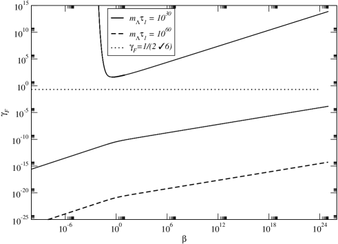
FIG. 8.: Contour plot of the function $\Upsilon(\beta,\gamma_{{}_{\rm F}})$ for $\Upsilon=10^{30}$ [solid lines] and $10^{60}$ [dashed line], i.e., respectively a particle life-time of the order of the age of the Universe, and of the proton life-time lower limit. Note that both top curves are indistinguishable due to the exponential behavior of $\Upsilon$ in $\gamma_{{}_{\rm F}}$. They turn out to be equivalent to the analytical requirement given by Eq. (97). Points above the highest curve and below the lowest curves satisfy the contraint. We also superimpose the conservative constraint (35) necessary for the existence of a massive bound state, the allowed region being above the dotted line.

On Fig. 8, we present the contour plot of the dimensionless function $\Upsilon(\beta,\gamma_{{}_{\rm F}})$, for $\Upsilon=10^{30}$ and $10^{60}$, which correspond respectively to a particle life-time of the order of the age of the Universe, and of the proton life-time lower limit. For $\beta\gtrsim 1$, there are in principle two allowed regions, corresponding to strong and weak coupling limits, i.e. $\gamma_{{}_{\rm F}}\gg 1$ and $\gamma_{{}_{\rm F}}\ll 1$. However, the lower bound on $\gamma_{{}_{\rm F}}$, which comes from the requirement that fermions are actually trapped on the brane, pushes the weak coupling allowed region to very high values of $\beta$, in practice $\beta\gtrsim 7.5\times 10^{57}$ for $\Upsilon=10^{30}$. Note also that this already rather extreme value is based on the conservative estimate given by Eq. (35).

For $\beta\lesssim 1$, the weak coupling region completely disappears, while the strong coupling allowed region shrinks rapidely: for $\beta\lesssim 8.5\times 10^{-3}$, the life-time cannot exceed the age of the Universe because $\gamma_{{}_{\rm F}}\gtrsim 10^{15}$. Considering $\beta\gtrsim 1$ therefore turns out to be the relevant limit if one wishes to have fermionic bound states living on the brane.

B Conclusion

In this article, we have considered fermions coupled to a Higgs field with a domain wall structure in a five dimensional anti-de Sitter spacetime. This domain wall can be thought of as a realization of a brane universe.

After, studying the domain wall configuration, we solved the Dirac equation and showed that there exists massive fermionic bound states trapped on the wall. We develop both analytic approximation to compute the mass spectrum and the tunneling time. This was compared to a full numerical integration of the dynamical equations that revealed the accuracy of our approximation scheme.

We recover the fact that massive fermions tunnel to the bulk [10]. Investigation in the parameter space shows that, for models satisfying the cosmological constraints, the relevant confinement life-time can be much greater that either the age of the Universe or the proton life-time. This was made possible by the derivation of the analytic estimate.

One of our central result is the derivation of an analytic mass spectrum for fermions trapped on a brane-like four dimensional spacetime. In particular, as could have been anticipated [13], it was shown that the allowed masses are quantized, with a spectrum varrying, in the strong coupling limit, as $\sqrt{n}$. Such a spectrum is indeed in contradiction with experimental measurements of particle masses [26], which is not surprising given the simplicity of the model. It however opens the possibility to build more realistic theories in which mass quantization would stem naturally from extra dimensions.

REFERENCES

- [1] L. Randall, R. Sundrum, Phys. Rev. Lett.83 (1999) 4690.
- [2] P. Binétruy, C. Deffayet, D. Langlois, Nucl. Phys. B 565 (2000) 269; C. Csáki, M. Graesser, C. Kolda, J. Terning, Phys. Lett. B 462 (1999) 34; J. M. Cline, C. Grojean, G. Servant, Phys. Rev. Lett.83 (1999) 4245; P. Binétruy, C. Deffayet, U. Ellwanger, D. Langlois, Phys. Lett. B 477 (2000) 285; P. Kraus, JHEP 9912 (1999) 11; T. Shiromizu, K. Maeda, M. Sasaki, Phys. Rev. D62 (2000) 024012; E. Flanagan, S. Tye, I. Wasserman, Phys. Rev. D62 (2000) 044039; R. Maartens, D. Wands, B. Bassett, I. Heard, Phys. Rev. D62 (2000) 041301. See also V. A. Rubakov, Large an infinte extra dimensions, hep-ph/0104152 and references therein.
- [3] J. Khoury, B. A. Ovrut, P. J. Steinhardt, N. Turok, The ekpyrotic universe: Colliding branes and the origin of the hot big bang, hep-th/0103239; J. Khoury, B. A. Ovrut, P. J. Steinhardt, N. Turok, A brief comment on ‘The Pyrotechnic universe’, hep-th/0105212; R. Y. Donagi, J. Khoury, B. A. Ovrut, P. J. Steinhardt, N. Turok, Visible branes with negative tension in heterotic M-theory, hep-th/0105199;
- [4] R. Kallosh, L. Kofman, A. Linde, Pyrotechnic universe, hep-th/0104073; R. Kallosh, L. Kofman, A. Linde, A. Tseytlin, BPS branes in cosmology, hep-th/0106241.
- [5] K. Akama, Lect. Notes Phys. 176 (1982) 267; V. A. Rubakov, M. E. Shaposhnikov, Phys. Lett. B 125 (1983) 136; M. Visser, Phys. Lett. B 159 (1985) 22.
- [6] G. W. Gibbons, D. L. Wiltshire, Nucl. Phys. B 287 (1987) 717 [hep-th/0109093].
- [7] B. Bjac, G. Gabadadzé, Phys. Lett. B 474 (2000) 282.
- [8] G. Dvali, M. Shifman, Phys. Lett. B 396 (1997) 64; ibid. 407 (1997) 452; G. Dvali, G. Gabadadzé, M. Shifman, Phys. Lett. B 497 (2001) 271; P. Dimopoulos, K. Farakos, A. Kehagias, G. Koutsoumbas, Lattice Evidence for Gauge Field Localization on a Brane, hep-th/0007079; M. J. Duff, J. T. Liu, W. A. Sabra, Localization of supergravity on the brane, hep-th/0009212; I. Oda, A New Mechanism for Trapping of Photon, hep-th/0103052, K. Ghoroku, A. Nakamura, Massive vector trapping as a gauge boson on a brane, hep-th/0106145; E. Kh. Akhmedov, Dynamical localization of gauge fields on a brane, hep-th/0107223.
- [9] R. Jackiw, C. Rebbi, Phys. Rev. D13 (1976) 3398.
- [10] S. L. Dubovsky, V. A. Rubakov, P. G. Tinyakov, Phys. Rev. D62 (2000) 105011.
- [11] J. Hisano, N. Okada, Phys. Rev. D61 (2000) 106003.
- [12] C. Ringeval, Fermionic massive modes along cosmic strings, hep-ph/0106179, Phys. Rev. D(2001) in press.
- [13] A. Neronov, Fermion masses and quantum numbers, gr-qc/0106092.
- [14] H. Lee, W. S. l’Yi, Domain walls stabilities, and the mass hierarchy of the Randall-Sundrum model, hep-th/0011144.
- [15] F. Bonjour, C. Charmousis, R. Gregory, Class. Quant. Grav. 16 (1999) 2427.
- [16] J. Polchinsky, String Theory, Vol. 2 (Cambridge University Press, Cambridge, UK, 1997).
- [17] N. D. Birrell, P. C. W. Davies, Quantum fields in curved space, (Cambridge University Press, Cambridge, UK, 1984).
- [18] S. Randjbar-Daemi, M. Shaposhnikov, Phys. Lett. B 492 (2000) 361.
- [19] M. Abramowitz, C.A. Stegun, Handbook of Mathematical Functions with Formulas, Graph, and Mathematical Tables (Dover Publications, 1972).
- [20] J. C. P. Miller, Tables of Weber Parabolic Cylinder Functions (Her majesty’s stationery office, London, UK, 1955).
- [21] I. S. Gradshteyn, I. M. Ryzhik, Table of Integrals, Series and Products (Academic Press, 1980).
- [22] B. Carter, J.-P. Uzan, Reflection symmetry breaking scenarios with minimal gauge form coupling in brane world cosmology, Nucl. Phys. B 606 (2001) 45.
- [23] R. Battye, B. Carter, A. Mennim, J.-P. Uzan, Einstein Equations for an asymmetric brane-world, Phys. Rev. D(2001) in press.
- [24] J. C. Long, A. B. Churnside, J. C. Price, Gravitational experiment below 1 Millimeter and comment on shielded Casimir backgrounds for experiments in the micron regime, Proceedings of the IXth Marcel Grossmann Meeting (Rome, 2–8 July 2000).
- [25] D. J. H. Chung, H. Davoudias, L. Everett, Phys. Rev. D64 (2001) 065002.
- [26] Particle Data Group, Eur. Phys. J. C 15 (2000) 1.