Mother Moose: Generating Extra Dimensions from Simple Groups at Large $N$

Abstract

We show that there exists a correspondence between four dimensional gauge theories with simple groups and higher dimensional gauge theories at large $N$. As an example, we show that a four dimensional ${\cal N}$=2 supersymmetric $SU(N)$ gauge theory, on the Higgs branch, has the same correlators as a five dimensional $SU(N)$ gauge theory in the limit of large $N$ provided the couplings are appropriately rescaled. We show that our results can be applied to the AdS/CFT correspondence to derive correlators of five or more dimensional gauge theories from solutions of five dimensional supergravity in the large t’Hooft coupling limit.

I Introduction

The idea that gauge theories in varying dimensions are intimately related has lead to new insights to our understanding of strongly coupled quantum field theories. One way to relate theories in differing dimensions is through the holographic AdS/CFT correspondence. Another way is to use the fact that one can trade dynamical degrees of freedom for additional dimensions. This result can be seen to be a simple consequence of effective field theory. If we consider a $d+1$ dimensional theory and compactify one dimension, then at distance scales large compared to the compactification radius the theory will necessarily look $d$ dimensional. The effects of the extra dimension are suppressed by powers of $ER$ and can be taken into account by adding higher dimensional local operators when integrating out Kaluza-Klein states according to a matching procedure. Given these facts, one can see that it is possible to reverse engineer this process and actually build an extra dimension by adding the necessary states to the $d$ dimensional action.

Recently, this idea has been implemented within the context of “moose” or “quiver” theories. These are theories whose gauge groups are chains of $SU(N)$’s which communicate to each other through matter in bi-fundamental representations. The authors of Refs. [1, 2] have shown that given a moose theory at some ultraviolet scale, symmetry breaking will naturally lead to a five dimensional $SU(N)$ gauge theory at scales well below the symmetry breaking scale. That is to say, there is an approximate equivalence between Greens functions calculated in the four dimensional theory which include a tower of massive states, and Greens functions calculated in a five dimensional theory. This construction allows for sensible UV limits of theories which appear to be higher dimensional in the IR. See also Refs. [3, 4] for related ideas.

In this paper we extend this equivalence in the limit of large $N$. In particular we will show that there are entire classes of $d$ dimensional theories with simple groups which, in the large $N$ limit, have the same correlation functions as $d+1$ dimensional theories. It would be a straightforward exercise to extend our results to construct $d+n$ dimensional theories. We then apply this idea to the AdS/CFT correspondence, and show that it is possible to derive correlators in higher dimensional ($d>4$) field theories from classical supergravity solutions in the background of spaces with stacks of separated D-3 branes.

The basic premise behind the generalization involves orbifolding field theories, which we briefly review in the next section. In Section III, we outline the construction of extra dimensions from lower dimensional field theories. The main part of the paper is contained in Section IV where we discuss a supersymmetric example. The procedure of generating additional dimensions provided several phenomenological applications [5, 6, 7, 8, 9, 10, 11], but we do not attempt to apply our work to model building. In Section V, we work out an explicit example where the AdS/CFT correspondence can be utilized to calculate correlators in a five dimensional theory with sixteen supercharges.

II Orbifolding

In the large $N$ limit it is possible to relate Greens functions for two disparate theories in a non-trivial fashion. In particular, it has been shown that planar diagrams of two theories related by orbifolding are identical when the gauge couplings are rescaled. Orbifolding a field theory [12, 13, 14, 15] entails removing a set of fields which are not invariant under certain discrete group transformations.

The orbifolding procedure works as follows. Consider a discrete group $G$, with $\Gamma$ elements, embedded in an $SU(\Gamma N)$ gauge theory. For each element of the discrete group form an $N$-fold copy of the regular representation $\gamma^{a}$. With a convenient choice of basis, this entails placing $d_{i}N$ copies of each irreducible representation of $G$ with dimension $d_{i}$ along the diagonal. This $N$-fold copy of the regular representation of $G$ forms a $\Gamma N\times\Gamma N$ matrix, which is an element of $SU(\Gamma N)$. The dimensionality works out because $\sum_{i}(d_{i})^{2}=\Gamma$. The fundamental $F$ and adjoint $A$ of the group therefore transform as

$$F\rightarrow\gamma^{a}F,~{}~{}~{}A\rightarrow\gamma^{a}A(\gamma^{a})^{\dagger}.$$ (1)

Orbifolding means that the “daughter theory” field content is obtained by keeping only fields invariant under the discrete transformation in Eq. (1). Moreover, the action is obtained from a “mother theory”action by setting to zero all terms that contain fields not invariant under such transformations. All terms in the action with fields removed by the orbifolding procedure are therefore discarded. For a more detailed description of the orbifolding procedure see Ref. [16]. To get a non-trivial orbifolding, i.e. one that does not lead to a daughter theory which is simply multiple copies of the mother, it is necessary to embed the discrete symmetry in global symmetry groups of the action, as we will see below.

It has been shown [15], that the correlation functions of the daughter theory are identical to those of the mother theory up to the following rescaling of the couplings $g_{m}\rightarrow g_{d}/\sqrt{\Gamma}$. This is a non-trivial result given that the loops of the mother theory incorporate fields which are not present in the daughter theory. The proof of the relation relies only on the fact that the leading order graphs in $1/N$ are planar. The correspondence is thus strictly true perturbatively. However, there is considerable evidence, especially in supersymmetric theories, that it works at the non-perturbative level as well [16, 17, 18]. Here we will utilize the orbifolding procedure to generate moose theories which, upon symmetry breaking, generate higher dimensional theories.

III Moosing

Consider a theory of $\Gamma$ $SU(N)$ gauge groups which are linked together by matter in the bi-fundamental representation. The theory may be depicted as in Figure 1, with each circle representing a gauge group and each line representing a matter multiplet [19]. An arrow pointing into (out of) a gauge group corresponds to a matter multiplet transforming in the (anti)fundamental representation of that particular gauge group. The gauge symmetry is broken down to the diagonal subgroup at scale $v$, when the bi-fundamental fields get expectation values. The bi-fundamental field may be either fundamental scalars or fermionic bound states. We could represent them as linear or non-linear sigma models. In the following we will use the linear realization, so the Lagrangian of the moose configuration is

$${\mathcal{L}}=\sum_{i=1}^{\Gamma}\,Tr\left(-\frac{1}{4g^{2}}F^{\mu\nu i}F_{\mu\nu}^{i}+(D^{\mu}U_{i})^{\dagger}D_{\mu}U_{i}\right)\,+\,\ldots,$$ (2)

where we have omitted the potential for the matter fields which is necessary for giving vevs to those fields. The covariant derivatives are defined as $D_{\mu}U_{i}=\partial_{\mu}U_{i}-iA^{i}_{\mu}U_{i}+iU_{i}A_{\mu}^{i+1}$. When all $U$’s obtain diagonal vevs, $U_{i}=v{\mathbf{1}}+\hat{U}_{i}$, this action is exactly the latticized version of the action of a compact $D+1$ dimensional $SU(N)$ gauge theory of radius $R=\Gamma a$ and lattice spacings $a=\frac{1}{gv}$. The $U$’s play the role of the link variable in the latticized new dimension.

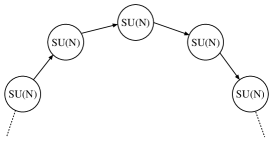
FIG. 1.: Typical moose diagram

At energy scales in the range $gv/\Gamma<<E<<gv$ the theory looks like a $D+1$ dimensional continuum gauge theory. This may be thought of as essentially the reverse process of Kaluza-Klein reduction. If we compactify a $D+1$ dimensional theory on a flat background then the $D$ dimensional action is just comprised of zero modes for the fields plus a tower of massive KK states with masses

$$m_{n}=\frac{2\pi n}{R}.$$ (3)

The moose is simply a construct which naturally leads to a tower of states, which in the above energy range, and for large enough $\Gamma$, approximately reproduce the spectrum of KK modes. Indeed, if we diagonalize the mass matrix for the gauge bosons in Eq.(2), we find [1, 2]

$$M_{n}^{2}=4g^{2}v^{2}sin^{2}\left(\frac{\pi n}{\Gamma}\right),$$ (4)

where $-\Gamma/2<n\leq\Gamma/2$. For $n<<\Gamma$ this approximates the above spectrum for the KK tower. Notice that the gauge coupling of the diagonal subgroup is given by

$$\frac{1}{g^{2}_{D}}=\frac{R}{g_{D+1}^{2}}.$$ (5)

It is simple to see how the extra-dimensional phase space is generated once the sum over the KK tower is performed. Consider two particle phase space for the scattering of a zero mode:

$$2PS\equiv\sum_{n}\int\frac{d^{d}k_{1}^{n}}{(2\pi)^{d-1}E_{1}^{n}}\frac{d^{d}k_{2}^{n}}{(2\pi)^{d-1}E_{2}^{n}}\delta^{(d)}(P-k_{1}^{n}-k_{2}^{n}),$$ (6)

where $E^{n}=\sqrt{k^{2}+m_{n}^{2}}$ is the energy of the $n$-th KK mode. In flat space K-K number is conserved, thus both final states have the same masses. In the limit where $\Gamma>>1$ we may replace the sum over KK modes by an integral such that

$$2PS \equiv \int dmdm^{\prime}\frac{{d^{d}k_{1}}}{(2\pi)^{d-1}E_{1}(m)}\frac{{d^{d}k_{2}}}{(2\pi)^{d-1}E_{2}(m)}\delta^{(d)}(P-k_{1}-k_{2})\delta(m-m^{\prime})$$ (7)

$$\propto \int\frac{{d^{d+1}k_{1}}}{(2\pi)^{d}E_{1}}\frac{{d^{d+1}k_{2}}}{(2\pi)^{d}E_{2}}\delta^{(d+1)}(P-k_{1}-k_{2}).$$ (8)

The second delta function in the first line enforces conservation of momentum in the extra dimension. This relation had to be true if the full exact KK tower were included, and is approximately true, up to power corrections, in the moose construction.

IV Extra Dimensions from Simple Groups

We would now like to combine these two techniques in such a way that we may generate an extra dimension from theories which are simpler than mooses. In particular, we would like to show that at large $N$ there are simple groups which, when Higgsed, generate extra dimensions. Here we will consider one simple supersymmetric example in four dimensions. In the supersymmetric case the role of the bi-fundamental field will be played by the scalar component of a chiral multiplet, but it is also possible to generate non-supersymmetric examples.

One might be concerned that the spontaneous symmetry breaking may destroy the simple relation between planar diagrams. It is important that the choice of the vev does not break the orbifold symmetry. This happens automatically if the fields which obtain vevs are those shared by the mother and daughter theories. Such fields transform trivially under the orbifold symmetry. The correspondence between orbifolded theories holds diagram by diagram. Given corresponding diagrams in unbroken phases, we can compare such diagrams in spontaneously broken phases. For the correspondence to go through in the broken phases of the theory we must impose the constraint that $gv$ be the same in the two theories. That is, $v_{m}=\sqrt{\Gamma}v_{d}$. This condition arises from that fact that, when the gauge fields are canonically normalized, an $n$ particle interaction vertex must scale as $g^{n-2}$ in order for the orbifold correspondence to hold[16].

We begin with an ${\mathcal{N}}=1$ supersymmetric $SU(\Gamma N)$ gauge theory with a chiral superfield $A$ in the adjoint representation. In principle we could add a superpotential for the field $A$, which can be made consistent with planarity in the large $N$ limit, but for simplicity we will set the superpotential to zero. Therefore this theory is equivalent to pure ${\cal N}=2$ SUSY Yang-Mills theory. In component form this theory has Lagrangian

$${\mathcal{L}}=\frac{1}{g^{2}}{\rm Tr}\left(-\frac{1}{4}F^{\mu\nu}F_{\mu\nu}-i\bar{\lambda}D\!\!\!\!/\lambda-i\bar{\psi}D\!\!\!\!/\psi+\mid\!\!D_{\mu}\phi\!\!\mid^{2}-\frac{1}{2}\left[\phi^{\dagger},\phi\right]^{2}-i\sqrt{2}[\lambda,\psi]\phi^{\dagger}-i\sqrt{2}[\bar{\lambda},\bar{\psi}]\phi\right),$$ (9)

where the gauge field and $\lambda$ are components of the vector multiplet, while $\psi$ and $\phi$ are components of the chiral multiplet $A$.

This theory has an extensive moduli space parameterized by the set of holomorphic gauge invariant polynomials. The independent gauge invariants are powers of the adjoint: ${\rm Tr}(A^{i})$, $i=2,\ldots,\Gamma N$. On the Coulomb branch the low energy effective action can be solved for up to higher derivative terms [20]. Here will be not be interested in the Coulomb branch but in the Higgs branch instead.

We consider orbifolding an $SU(\Gamma N)$ by the discrete subgroup $Z_{\Gamma}$. The gauge indices of all the multiplets will transform according to Eq. (1) under this orbifolding. In addition, we will embed the $Z_{\Gamma}$ discrete symmetry into a $U(1)_{A}$ global symmetry of the chiral superfield. The $U(1)_{A}$ rotates the adjoint matter field by a phase, so it is an “adjoint number” symmetry. This $U(1)$ symmetry is anomalous with a $Z_{2\Gamma N}$ subgroup preserved by instantons. We embed the “orbifold” symmetry $Z_{\Gamma}$ into the non-anomalous subgroup of $U(1)_{A}$.

Under orbifolding the $SU(\Gamma N)$ gauge group breaks up into the product group $SU(N)^{\Gamma}$. There are $\Gamma-1$ additional $U(1)$ gauge symmetries preserved by the orbifolding. With our choice of matter content these $U(1)$ symmetries will be anomalous, but do not contribute in the large N limit. The matter fields which are kept in the daughter theory are those which are invariant under the transformation

$$(\psi,\phi)\rightarrow r^{a}\gamma_{a}(\psi,\phi)(\gamma_{a})^{\dagger},$$ (10)

where $r^{a}$ is a pure phase, and has the effect of pushing the invariant fields to the right of the diagonal. Schematically, the orbifolding gives

$$A\rightarrow\left(\begin{array}[]{ccccc}&A_{1}&&\ldots&\\ &&A_{2}&\ldots&\\ \vdots&\vdots&\vdots&\ddots&\vdots\\ &&&\ldots&A_{\Gamma-1}\\ A_{\Gamma}&&&\ldots&\end{array}\right),$$ (11)

where $A_{i}$ are the daughter theory bi-fundamentals transforming under neighbor $SU(N)$ groups. In performing the orbifolding we have reduced the number of supersymmetries to four (we will regain supersymmetry in the low energy limit where the theory looks five dimensional). This is precisely the theory illustrated by the moose diagram shown in Figure 1. The Seiberg-Witten curves for the Coulomb branch of this theory were derived in Ref. [21].

For our purposes we will choose a point on the moduli space corresponding to a partial Higgsing of the gauge group. Our choice of a points on the moduli space is such that, in the daughter theory, the bi-fundamental scalars each get equal expectation values. The corresponding vev in the mother theory is of the form

$$\langle A\rangle=v\left(\begin{array}[]{ccccc}&{\mathbf{1}}&&\ldots&\\ &&{\mathbf{1}}&\ldots&\\ \vdots&\vdots&\vdots&\ddots&\vdots\\ &&&\ldots&{\mathbf{1}}\\ {\mathbf{1}}&&&\ldots&\end{array}\right),$$ (12)

where each ${\mathbf{1}}$ represents an $N\times N$ identity matrix. This choice of vevs is part of the moduli space of both mother and daughter theories. In the daughter theory all vevs are aligned and proportional to the identity, so they are D-flat. They correspond to baryonic flat directions. In the mother theory it is easy to check that $\langle A\rangle\,\langle A^{\dagger}\rangle-\langle A^{\dagger}\rangle\,\langle A\rangle=0$, therefore all D terms vanish [22].

Breaking the $SU(\Gamma N)$ gauge symmetry with the vev of Eq. (12) leaves the mother theory with an $SU(N)^{\Gamma}$ gauge symmetry. It is easy to see the breaking pattern after diagonalizing the vev in the mother theory

$$\langle A\rangle=v\left(\begin{array}[]{ccccc}{\mathbf{1}}&&&\ldots&\\ &\omega\,{\mathbf{1}}&&\ldots&\\ &&\omega^{2}\,{\mathbf{1}}&\ldots&\\ \vdots&\vdots&\vdots&\ddots&\vdots\\ &&&\ldots&\omega^{\Gamma-1}\,{\mathbf{1}}\end{array}\right),$$ (13)

where $\omega^{\Gamma}=1$. In this new basis it is easy to read of the spectrum of the mother theory. The diagonal $N\times N$ blocks correspond to unbroken $SU(N)^{\Gamma}$, each with a massless adjoint superfield. In addition, there are $\Gamma-1$ massless $U(1)$ gauge bosons as well as $\Gamma-1$ massless chiral superfields which are singlets under all the unbroken gauge groups. These fields do not contribute at the leading order in $N$. The off-diagonal $N\times N$ blocks correspond to massive vector superfields. The masses of the fields in different blocks are

$$M^{2}=4g^{2}_{m}v^{2}_{m}\left(\begin{array}[]{ccccc}0&\sin^{2}(\pi/\Gamma)&\sin^{2}(2\pi/\Gamma)&\ldots&\sin^{2}(\pi/\Gamma)\\ \sin^{2}(\pi/\Gamma)&0&\sin^{2}(\pi/\Gamma)&\ldots&\sin^{2}(2\pi/\Gamma)\\ \sin^{2}(2\pi/\Gamma)&\sin^{2}(\pi/\Gamma)&0&\ldots&\sin^{2}(3\pi/\Gamma)\\ \vdots&\vdots&\vdots&\ddots&\vdots\\ \sin^{2}(\pi/\Gamma)&\sin^{2}(2\pi/\Gamma)&\sin^{2}(3\pi/\Gamma)&\ldots&0\end{array}\right).$$ (14)

The vev of Eq. (12) breaks the daughter theory to a diagonal $SU(N)$ with a gauge coupling $g_{diag}^{2}=g_{d}^{2}/\Gamma$. In addition there is a massless chiral superfield transforming in the adjoint of the diagonal $SU(N)$. The massless gauge bosons are accompanied by a tower of massive gauge bosons with masses

$$m^{2}_{k}=4g^{2}_{d}v^{2}_{d}\sin^{2}(\frac{\pi k}{\Gamma}).$$ (15)

Note that if we want to keep the masses fixed as we take the t’Hooft limit $N\rightarrow\infty$ with $g^{2}N$ fixed, we need to simultaneously rescale the vevs and keep $v^{2}/N$ unchanged. From now on, we will assume that $gv$ is held fixed in the large $N$ limit. There are also $\Gamma$ massless singlet chiral superfields, which are the parts of the link fields not eaten by the super-Higgs mechanism when breaking to the diagonal subgroup.

Comparing Eqs. (14) and (15) we obtain the same mass spectrum if $v_{m}=v_{d}\sqrt{\Gamma}$, in concordance with our previous statement of the equality of $gv$ in the two theories. In the interesting limit of $k<<\Gamma$ we get $m_{k}\simeq k\,(2\pi gv)/\Gamma$. If we define the lattice spacing as $a^{-1}=gv$ and the compactification radius as $R=\Gamma a$, then we have correctly reproduced the KK tower for a compactified flat extra dimension. The pattern of orbifolding and symmetry breaking is shown in Figure 2.

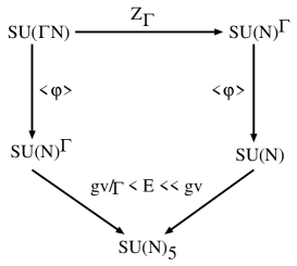
FIG. 2.: The pattern of orbifolding and symmetry breaking. The mother theory is on the left and the daughter on the right.

In order to compare the correlators of the mother and daughter we need to identify the corresponding fields in the two theories. It is only for these shared fields that we can expect the equality of correlators. In the basis defined by Eq. (11) the correspondence between the fields is most transparent. The corresponding mother’s and daughter’s fields reside at the same positions. Vectors live on the diagonal blocks and scalars live on blocks above the diagonal. Since in the mother we changed the basis by diagonalizing vevs in Eq. (13), we need to perform the same transformation on all the fields.

Let us start with the massless gauge multiplet of the daughter theory. This multiplet, after the breaking of the $SU(N)^{\Gamma}\rightarrow SU(N)_{diag}$ symmetry, is a linear combination of all $SU(N)^{\Gamma}$ fields with the same coefficient for each field. The corresponding field in the mother theory is the same linear combination of $SU(N)^{\Gamma}$ fields on the diagonal. For this special linear combination there is no change induced in going from basis defined by Eq. (12) to the one defined by Eq. (13). The properly normalized linear combination of fields is

$$A^{a}_{diag}=(A^{a}_{1}+A^{a}_{2}+\ldots+A^{a}_{\Gamma})/\sqrt{\Gamma}.$$ (16)

Therefore, the coupling of the diagonal subgroup is $g/\sqrt{\Gamma}$.

As far as the massive multiplets are concerned each $N\times N$ block of the mother theory transforms as an adjoint under the diagonal subgroup since bi-fundamentals of $SU(N)^{\Gamma}$ transform as adjoints under the diagonal subgroup. With this identification we begin to see why the correlators are identical up to a rescaling. At each mass level of the mother theory there are $\Gamma$ adjoints of the diagonal subgroup. However, each of the adjoints couples with the reduced coupling $g/\sqrt{\Gamma}$, so the two compensate. The rescaling of the coupling then compensates for the factor of $\sqrt{\Gamma}$ in the daughter theory coupling. In the large $N$ limit, additional massless fields whose number does not grow with $N$ become irrelevant. Since the spectra of the mother and daughter differ only by $O(\Gamma)$ fields, these theories have identical behavior for large $N$.

The massive vector multiplets in the daughter, again, correspond in the mother theory to linear combinations of fields. At mass level $k$ these are

$$A^{a}_{k}=(A^{a}_{1}+\omega^{k}A^{a}_{2}+\omega^{2k}\ldots+\omega^{k(\Gamma-1)}A^{a}_{\Gamma})/\sqrt{\Gamma}$$ (17)

in the daughter theory, as well as in the mother theory before diagonalizing the vev. When changing to the basis defined by Eq. (13) we need to appropriately transform this linear combination. It turns out that in the new basis the linear combinations no longer involves fields residing in the diagonal blocks, instead it involves all fields from blocks parallel to the diagonal. The linear combination includes vector fields from each $N\times N$ block with a given mass as displayed in Eq. (14). For the chiral superfields the linear combinations have different coefficients than those for the vector fields with the same mass. However, in the basis with the diagonal vev the linear combination of scalars also involves all fields in the appropriate blocks parallel to the diagonal. This is, of course, expected since the vector and chiral multiplets must combine into irreducible massive vector multiplets.

We can single out the diagonal subgroup of the mother theory, for which correlators look five dimensional, in several ways. First, we can impose a discrete symmetry that identifies $\Gamma$ $SU(N)$ factors. Alternatively, in the mother theory we can add a small diagonal vev with magnitude $v^{\prime}$, which breaks $SU(N)^{\Gamma}$ to the diagonal. When $v^{\prime}\ll v$ the splittings due to $v^{\prime}$ are negligible compared to the K-K splittings induced by $v$. Thus, we get $\Gamma$ nearly degenerate adjoints of the diagonal subgroup at each mass level $gv|\sin(\pi k/\Gamma)|$.

As we already mentioned, one can extend this construction to generate more dimensions by orbifolding a simple group. For example, an $SU(\Gamma^{2}N)$ theory with two adjoint chiral superfields can be orbifolded by a $Z_{\Gamma}\times Z_{\Gamma}$ discrete symmetry. We assign the transformation properties of the two chiral fields similar to Eq. (10), such that each of them picks a phase under one of $Z_{\Gamma}$ factors. The daughter theory resembles a two dimensional lattice, so with appropriate vevs both mother and daughter generate two extra dimensions.

For the daughter theory to look five dimensional we must restrict ourselves to the regime

$$g_{d}v_{d}/\Gamma<<E<<g_{d}v_{d}.$$ (18)

Now we must ask, what does the mother theory look like at these energy scales? We would expect that at some scale, $\Lambda_{m}$, the mother theory will get strong, and will most likely undergo a phase transition. However, the orbifold correspondence is blind to such effects. That is, the correspondence tells us that given the Greens function in the mother theory we can get the Greens functions in the daughter by simply making the replacement $g_{m}\rightarrow g_{d}/\sqrt{\Gamma}$, or vice versa. This statement is independent of scales. What does this mean in terms of our correspondence? It would seem that we are allowed to take the mother theory to be as weakly coupled or as strongly coupled as we wish and that in either case we can still equate its Greens functions with those of the 5-d theory. However, in order for the daughter theory to look five dimensional, we can only study energy scales with $E>>gv_{d}/\Gamma$. We are free to take $\Gamma$ to be as large as we wish, thus studying the theories at arbitrarily large distances. However, the four dimensional mother theory will get its coupling rescaled by $1/\sqrt{\Gamma}$, so it will remain weak in the regime where the daughter looks five dimensional. This had better be the case since the five dimensional theory is weakly interacting in the IR. Indeed, the gauge interaction in five dimensions is irrelevant and the theory is IR free. In the context of the four dimensional theory this can be seen from the fact that as we lower the energy scale more and more KK modes are decoupling and thus the interaction is getting weaker. So the effective coupling will scale with $E\Gamma/(gv)$, as one would expect for a compactified five dimensional theory.

V Gauge Gravity Correspondence in Five Dimensions

Suppose we start with an $SU(\Gamma N)$ mother theory which is ${\cal N}=4$ supersymmetric. By embedding the discrete orbifold group inside the $SU(4)$ R symmetry we may relate the mother theory correlation functions to those of an ${\cal N}=2$ (or ${\cal N}=1,0$) supersymmetric daughter theory. Given that the mother theory is finite and has vanishing beta function, the daughter theory must, in the large $N$ limit, be finite as well. In this section, we will assume that the mother is orbifolded to an ${\cal N}=2$ daughter. We can achieve that by embedding $Z_{\Gamma}$ in the R symmetry with matrix $diag(\omega,\omega^{*},1,1)$ acting on the fundamental representation of $SU(4)_{R}$. The matter content of the daughter is composed of $\Gamma$ vector multiplets and $\Gamma$ bi-fundamental hyper-multiplets. In terms of the ${\cal N}=2$ multiplets, the theory has identical structure as the moose depicted in Figure 1 (with links now unoriented). Moving away from the origin of moduli space onto the Higgs branch we may moose the theory in the same way as in the example discussed above. The resulting five dimensional theory has 16 supercharges. The mother starts out as a superconformal theory, however going out on the Higgs branch maintains 16 supercharges. The daughter has eight supercharges and additional accidental supersymmetry at low energies.

In the following, we will outline how the AdS/CFT correspondence might be used to calculate correlators of five dimensional field theory. The AdS/CFT correspondence is commonly used for field theories with large t’Hooft coupling. One might worry that the discussion of the spontaneous symmetry breaking is only applicable at weak coupling. However, in ${\cal N}=4$ theory all masses are related to the central charges of the supersymmetric algebra and are BPS saturated. Thus, the tree-level results are not renormalized and one obtains the same KK tower for any of the value of the gauge coupling.

The deformation onto the Higgs branch yields a non-trivial RG flow to an IR fixed point, which is reached once we integrate out all the KK modes. This scenario has an interesting interpretation in the AdS/CFT correspondence. Recall that the $D3$ brane metric in type IIB string theory is given by

$$ds^{2}=H^{-1/2}\eta_{\mu\nu}dx^{\mu}dx^{\nu}+H^{1/2}\delta_{ij}dy^{i}dy^{j},$$ (19)

with the $x^{\mu}$ coordinates spanning the world-volume of the D brane and $y^{i}$ span ${\bf R}^{6}$. H is given by

$$H=h+\frac{R^{4}}{r^{4}},$$ (20)

where $R^{4}\equiv 4\pi g_{s}\alpha^{\prime}N$, $r^{2}=\delta_{ij}y^{i}y^{j}$, and $h=1$. Near $r\rightarrow 0$, one approaches a non-singular horizon, and the space is locally $AdS_{5}\times S^{5}$. Whereas, in the limit $r\rightarrow\infty$ approaches 10 dimensional flat space.

The case of $h=0$, which is $AdS_{5}\times S_{5}$ for all $r$, is holographically described by the ${\cal N}=4$ super-conformal field theory, whereas the $h=1$ case retains 16 supercharges but is no longer conformal. It flows in the IR ($r\rightarrow 0$) to the $h=0$ case. The $h=1$ case has been conjectured to be dual to a super-conformal theory perturbed by a dimension eight operator [23, 24]. It turns out that this dimension eight operator is the most relevant operator induced by integrating out massive states in a Higgsed theory [24, 25].

We wish to Higgs the $SU(\Gamma N)$ mother theory, in the fashion described in the previous section. This may be accomplished by separating the stack of $\Gamma N$ D3 branes, leaving the geometry

$$H(y)=h+4\pi g_{s}\alpha^{\prime}\sum_{i=1}^{k}\frac{N_{i}}{\mid\vec{y}-\vec{a_{i}}\mid^{4}},$$ (21)

where $N_{i}$ are the number of D3 branes places at position $\vec{a}_{i}$ in the transverse space, and $\sum_{i=1}^{k}N_{i}=\Gamma N$. This solution breaks the $SU(4)$ R symmetry but preserves the 16 supercharges. The $\vec{a}_{i}$ correspond to the diagonal vevs of the six real adjoint scalars. The above brane configuration is only applicable at small values of the string coupling, so it is not apparent how to describe weakly coupled field theories this way.

Let us now consider the symmetry breaking pattern required for the moose constructions described in Eq. (13). In this case there are only two linearly independent vevs of the real scalar adjoints. One of these fields has vevs proportional to the real parts of $\omega^{k}$, while the other to the imaginary parts, where $k=0,\ldots,\Gamma-1$. This means that we can place all branes in just two transverse directions. In field theory this reflects the breaking of the $SU(4)\sim SO(6)$ R symmetry to $SO(4)$. We pick out two of the transverse directions, say $y^{5}$ and $y^{6}$ and place $\Gamma$ groups of $N$ branes with coordinates

$$a^{5} \propto v\,\{1,\cos(2\pi/\Gamma),\cos(4\pi/\Gamma),\ldots,\cos(2\pi(\Gamma-1)/\Gamma)\},$$ (22)

$$a^{6} \propto v\,\{0,\sin(2\pi/\Gamma),\sin(4\pi/\Gamma),\ldots,\sin(2\pi(\Gamma-1)/\Gamma)\}.$$ (23)

As might have been anticipated, the branes are arranged along the perimeter of a circle. Similar dualities of five dimensional field theories can be obtained from the orbifolds of the $AdS\times S^{5}$ space, which were described in Refs. [12, 13, 14, 15].

The field theory dual of this brane construction corresponds, by orbifolding at large $N$, to a five-dimensional theory. While the four dimensional coupling does not run, the effective coupling, which accounts for the fact that as we flow into the IR more and more KK modes are decoupling, becomes weaker. This is consistent with the five dimensional interpretation of the theory, where the coupling is an irrelevant operator at the classical level.

The five-dimensional field theory interpretation only applies for energies in the range $gv/\Gamma<<E<<gv$. For the supergravity approximation in the AdS/CFT correspondence to be trustworthy, the AdS curvature scale must be small compared to the Planck scale. This corresponds to taking $g_{m}\sqrt{N\Gamma}>>1$. The daughter’s coupling is $g_{m}\sqrt{\Gamma}$, but for the five dimensional theory the relevant coupling is that of the diagonal subgroup. Therefore, the effective coupling in the five-dimensional theory is

$$(ER)\frac{g^{2}_{d}N}{16\pi^{2}}=\frac{g^{2}_{m}N}{16\pi^{2}}\frac{E\Gamma}{g_{m}v_{m}}.$$ (24)

The five-dimensional interpretation makes sense only for energies below the cut-off, that is in the region where the loop expansion parameter in the effective theory is less than one. Thus, the energy range must be restricted to

$$g_{m}v_{m}/\Gamma<<E<g_{m}v_{m}\frac{16\pi^{2}}{g^{2}_{m}N\Gamma},$$ (25)

where the lower bound is equal to the mass of the lightest KK state. If $g_{m}\sqrt{N\Gamma}<4\pi$ then our AdS/CFT dual can be interpreted as a five-dimensional field theory in the full energy range $gv/\Gamma<<E<<gv$ accessible to moose constructions. If the t’Hooft coupling is large $g_{m}\sqrt{N\Gamma}>4\pi$ then only part of that energy range remains below the cut-off. Of course, we cannot take the t’Hooft coupling to be too small or string corrections will become important. It is not difficult to generalize this construction to allow for a correspondence between $AdS_{5}$ and gauge theories of dimension higher than five. One needs to simply choose the appropriate $D$ brane configurations in the bulk. It would be interesting to search for classical solutions in these non-trivial backgrounds to test the correspondence with higher dimensional field theories.

Note added: After completing this work we were made aware of Refs. [26, 27] which have considerable overlap with Section V.

- [1] N. Arkani-Hamed, A. G. Cohen and H. Georgi, Phys. Rev. Lett. 86, 4757 (2001), hep-th/0104005.
- [2] C. T. Hill, S. Pokorski and J. Wang, hep-th/0104035.
- [3] M. B. Halpern and W. Siegel, Phys. Rev. D 11, 2967 (1975).
- [4] C. Castro, hep-th/0106260.
- [5] N. Arkani-Hamed, A. G. Cohen and H. Georgi, Phys. Lett. B 513, 232 (2001), hep-ph/0105239.
- [6] H. Cheng, C. T. Hill and J. Wang, hep-ph/0105323.
- [7] C. Csaki, J. Erlich, C. Grojean and G. D. Kribs, hep-ph/0106044.
- [8] H. C. Cheng, D. E. Kaplan, M. Schmaltz and W. Skiba, Phys. Lett. B 515, 395 (2001), hep-ph/0106098.
- [9] C. Csaki, G. D. Kribs and J. Terning, hep-ph/0107266.
- [10] H. Cheng, K. T. Matchev and J. Wang, hep-ph/0107268.
- [11] N. Arkani-Hamed, A. Cohen and H. Georgi, hep-th/0108089.
- [12] S. Kachru and E. Silverstein, Phys. Rev. Lett. 80, 4855 (1998), hep-th/9802183.
- [13] M. Bershadsky, Z. Kakushadze and C. Vafa, Nucl. Phys. B 523, 59 (1998), hep-th/9803076.
- [14] Z. Kakushadze, Nucl. Phys. B 529, 157 (1998), hep-th/9803214.
- [15] M. Bershadsky and A. Johansen, Nucl. Phys. B 536, 141 (1998), hep-th/9803249.
- [16] M. Schmaltz, Phys. Rev. D 59 (1999) 105018, hep-th/9805218.
- [17] J. Erlich and A. Naqvi, hep-th/9808026.
- [18] M. J. Strassler, hep-th/0104032.
- [19] H. Georgi, Nucl. Phys. B 266, 274 (1986).
- [20] N. Seiberg and E. Witten, Nucl. Phys. B 426, 19 (1994) [Erratum-ibid. B 430, 485 (1994)], hep-th/9407087; P. C. Argyres and A. E. Faraggi, Phys. Rev. Lett. 74, 3931 (1995), hep-th/9411057.
- [21] C. Csaki, J. Erlich, D. Freedman and W. Skiba, Phys. Rev. D 56, 5209 (1997), hep-th/9704067.
- [22] I. Affleck, M. Dine and N. Seiberg, Nucl. Phys. B 256 (1985) 557.
- [23] S. S. Gubser and A. Hashimoto, Commun. Math. Phys. 203, 325 (1999), hep-th/9805140.
- [24] K. Intriligator, Nucl. Phys. B 580, 99 (2000), hep-th/9909082.
- [25] M. S. Costa, Phys. Lett. B 482, 287 (2000) [Erratum-ibid. B 489, 439 (2000)], hep-th/0003289.
- [26] K. Sfetsos, JHEP 9901, 015 (1999), hep-th/9811167.
- [27] K. Sfetsos, hep-th/0106126.