D-branes in Nonabelian Orbifolds with Discrete Torsion

Abstract:

We study IIB string theory on the orbifold ${\mathbb{R}}^{8}/\Gamma$ with discrete torsion where $\Gamma$ is an arbitrary subgroup of $U(4)$. We extend some previously known identities for discrete torsion in abelian groups to nonabelian groups. We construct explicit formulas for a large class of fractional D-brane states and prove that the physical states are classified by projective representations of the orbifold group as predicted originally by Douglas. The boundary states are found to be linear combinations of Ishibashi states with the coefficients being characters of the projective representations.

1 Introduction

In this paper we will study certain orbifolds of type IIB string theory with discrete torsion and characterize D-brane states in these theories. Type IIB in ten dimensions is already an orbifold, namely of the GSO group. We further mod out by a geometrical orbifold group, $\Gamma_{0}\subset U(4)\subset SO(8)$ to get type IIB on ${\mathbb{R}}^{8}/\Gamma_{0}$. For a given orbifold group there are various possibilities for a consistent theory, these possibilities differ by discrete torsion [1, 2]. An effective approach to studying D-branes in string theory – which we will follow – is provided by the boundary state formalism [3, 4], a review of which can be found e.g. in [5, 6, 7]. The study of D-brane states in abelian orbifolds with discrete torsion was initiated by Douglas and Fiol [8, 9] who conjectured that D-branes were classified by projective representations of the orbifold group. Later more work was done in various examples [10, 11, 12, 13, 14, 15, 16, 17] and this picture was confirmed in the abelian case. For results on orbifolds without discrete torsion, see for example [18, 19, 20, 21, 22, 23].

The aim of this paper is to describe the D-branes in nonabelian orbifold theories with discrete torsion and prove that they are given in terms of projective representations of the orbifold group. In order to do this we present explicit formulas for the relation between discrete torsion in Vafa’s sense and the cocycles of projective representations. In particular we propose the following relation between the discrete torsion and the cocycles in the general (nonabelian) case:

$$\varepsilon(h,g)=\frac{c(ghg^{-1},g)}{c(g,h)}\,.$$

We write down explicit formulas for the boundary states of the D-branes, impose orbifold invariance and use open–closed string duality to impose a physical condition. We then show that this condition is solved by characters of projective representations exactly as predicted by Douglas. It turns out that for $\Gamma_{0}\subset U(4)\subset SO(8)$ certain boundary states can be written in a uniform way that does not require fermionic zero modes to be treated separately. In order to classify the boundary states it is necessary to fix various phases in the orbifold action on the closed string Hilbert space. We make the assumption, which was also employed in [24, 25], that one of the orbifold theories contain all the fractional D-instantons and anti D-instantons as in [26]; in other words there should exist a theory in which D-instantons are classified by ordinary representations. This assumption partly determines the unknown phases while the rest can be fixed by introducing discrete torsion in the product of the GSO group and the geometrical group. Having fixed these phases the spectrum of open string states can be read off and we prove that the consistency conditions are solved by projective characters. Our result is the following. Let $|\,h;S,\eta\,\rangle\!\rangle$ denote the Ishibashi state in the $h$-twisted sector solving the gluing condition $(S,\eta)$ (see the text for the precise definitions) and let $\Gamma_{S}\subset\Gamma$ be the subgroup of the orbifold group containing elements which leave the gluing condition $(S,\eta)$ invariant. Then the following boundary states define D-branes:

$$|\,R\,;S\,\rangle\!\rangle =\frac{1}{\sqrt{|\Gamma|}}\sum_{[f]\in\Gamma/\Gamma_{S}}\sum_{h\in\Gamma_{S}}\mbox{Tr}(\gamma_{R}(h))\,\varepsilon(h,f)\,f|\,h;S,+\,\rangle\!\rangle\,,$$

where $R:h\mapsto\gamma_{R}(h)$ is a projective representation of $\Gamma_{S}$.

The paper is organized as follows: In section 2 we specify the orbifold theories that we are interested in and discuss discrete torsion. In section 3 we construct boundary states explicitly and impose invariance of these under the orbifold group, both with and without discrete torsion. In section 4 we impose open string–closed string duality on the boundary states in order to determine the spectrum of physical states. We show that the spectrum is determined by projective representations of certain subgroups of the orbifold group. In section 5 we conclude.

2 Orbifold theories

We shall determine boundary states in various orbifolds of superstring theory. For simplicity we will specialize to type IIB theory. We start with the ten-dimensional GSO-unprojected superstring and include the GSO in the orbifold group.

We shall be working in light cone gauge with $0,1$ being the light-cone coordinates and let the orbifold group act on the remaining 8 coordinates only. We require that the action of the elements of the orbifold group $g\in\Gamma$ has the following form:

$$\begin{split}X^{\mu}\rightarrow A^{\mu\nu}(g)X^{\nu}\qquad\qquad\qquad\qquad&\psi_{L}^{\mu}\rightarrow-A_{L}^{\mu\nu}(g)\psi_{L}^{\nu}\\ &\psi_{R}^{\mu}\rightarrow-A_{R}^{\mu\nu}(g)\psi_{R}^{\nu}\,.\end{split}$$ (1)

where $\mu=2\ldots 9$, $A(g)$ is an $U(4)\subset SO(8)$ matrix and $A_{L}(g),A_{R}(g)$ are equal to $A(g)$ up to a possible sign. A generic geometric orbifold could be obtained by choosing a subgroup $\Gamma\subset SO(8)$. In this paper however, we chose to restrict to groups $\Gamma$ which respect a complex structure on ${\mathbb{R}}^{8}$ thus are embedded in a subgroup $U(4)\subset SO(8)$. These orbifolds preserve some spacetime supersymmetry and the use of the complex structure makes our analysis more straightforward. Also, we shall focus on boundary states which respect this structure. The transformation of the fermions is determined by the transformation of the bosons from worldsheet supersymmetry up to a sign. For example the usual geometric orbifold would correspond to $A_{L}=A_{R}=A$ while the four elements used in the GSO projection have $A=1\mbox{l}$. We have also included a minus sign for the fermions so that the NSNS sector corresponds to the untwisted sector thus reflecting the periodicity on the complex plane.

We will always impose the GSO projection, therefore the most general form of the orbifold group is

$$\Gamma =\Gamma_{0}\times({\mathbb{Z}}_{2}^{(L)}\times{\mathbb{Z}}_{2}^{(R)})_{GSO},$$

where $\Gamma_{0}$ contains elements with $A_{L}=A_{R}=A$ in (1). It is important to realize that the orbifold is not completely defined by (1) for the following reason. The orbifold is defined by first introducing twisted sectors, one for each group element. The quantization of these sectors gives rise to a covering Hilbert space whose $\Gamma$ invariant subspace defines the physical Hilbert space. To keep the $\Gamma$ invariant subspace it is necessary to define an action of $\Gamma$ on each twisted sector. Each twisted sector is a Fock space where the tower of states can be obtained by acting with the raising operators from $X^{\mu}$ and $\psi^{\mu}$ on a lowest weight state. (1) defines the action of $\Gamma$ on the raising operators but not on the lowest weight state. In the case of zero modes there are many possible choices of the lowest weight state, but any choice will do, because the zero modes will transform these among themselves. To define the action of $\Gamma$ on the large Hilbert space it is thus necessary to define the action of $\Gamma$ on each of the lowest weight states. Furthermore this action has to be defined such that $\Gamma$ is a symmetry of the theory, i.e. $\Gamma$ is a symmetry of the OPE. The $\Gamma$ invariant subspace then defines a unitary, modular invariant string theory.

Two questions are inevitable at this point: does the orbifold exist at all and is it unique? To our knowledge no one has proven that the orbifold exists for all $\Gamma$, but in many special cases it is known, of course. It could be checked explicitly but since it is out of the main course of this paper we will refrain from this and just assume that the orbifold exists. Alternatively one could say that our results about boundary states are only valid when the orbifold exists.

The uniqueness issue has been studied initially by Vafa [1]. In general it is not unique and the non-uniqueness is classified by discrete torsion as we will describe in the next subsection.

2.1 Discrete Torsion

Given an orbifold of type IIB/$\Gamma$ one can possibly define other related theories. The original orbifold is defined by having an action of $\Gamma$ on the covering Hilbert space including all twisted sectors and restricting to $\Gamma$-invariant states. The projection operator onto the physical subspace is given by

$$P=\frac{1}{|\Gamma|}\sum_{g\in\Gamma}g\,.$$

One can modify this theory by introducing discrete torsion [1] as follows. One defines new projection operators for each twisted sector:

$$P_{h}=\sum_{g\in\Gamma}\varepsilon(h,g)g\,,$$

where $h\in\Gamma$ is the twist and $\varepsilon(h,g)$ are complex numbers of unit norm. The physical states are the ones that are invariant under these projection operators. Remark that in general $P_{h}$ maps a state twisted by $h$ into a linear combination of states twisted by elements in the same conjugacy class as $h$.

Another way of understanding discrete torsion is as a redefinition of the elements of $\Gamma$. In the sector twisted by $h$ the redefinition is given by $\widehat{g}=\varepsilon(h,g)g$ with some conditions on $\varepsilon$. One comes from the fact that the redefined group elements form a representation of $\Gamma$, i.e.

$$\widehat{g_{2}g_{1}}=\widehat{g_{2}}\widehat{g_{1}}$$

Applying both sides to a state $|\,h\,\rangle$ which is twisted by $h$ and remembering that $g_{1}|\,h\,\rangle$ is twisted by $g_{1}hg_{1}^{-1}$ one gets that

$$\varepsilon(h,g_{2}g_{1})=\varepsilon(g_{1}hg_{1}^{-1},g_{2})\varepsilon(h,g_{1})\,,$$ (2)

Another condition comes from modular invariance of the torus amplitude [1] which requires that $\varepsilon$ obey

$$\varepsilon(g,h) =\varepsilon(g^{a}h^{b},g^{c}h^{d}),\qquad\mbox{where}\qquad\left(\begin{array}[]{cc}a&b\\ c&d\end{array}\right)\in SL(2,{\mathbb{Z}})\qquad\mbox{and}\qquad gh=hg\,.$$ (5)

Note that this only applies to commuting elements $g,h$, because there is no torus amplitude with noncommuting twist along the two directions. For noncommuting elements $g,h$, we have

$$\widehat{g}|\,h\,\rangle=\varepsilon(h,g)g|\,h\,\rangle=\varepsilon(h,g)|\,ghg^{-1}\,\rangle\,,$$

where $|\,k\,\rangle$ is some state in the sector twisted by $k$. We see that multiplying $|\,h\,\rangle$ by a phase changes $\varepsilon(h,g)$ by a phase; $\varepsilon$ is thus basis dependent to a certain degree. Of course $\varepsilon$’s that only differ in this way should be identified. For commuting elements this does not happen since both sides of the equation contain $|\,h\,\rangle$ thus for abelian groups $\varepsilon$ is independent of the choice of basis.

The set of $\widehat{g}$ constitute a group isomorphic to $\Gamma$ with another action on the Hilbert space but the same action on the fields $X^{\mu}$ and $\psi^{\mu}$. It is thus not well defined to ask whether an orbifold has discrete torsion. The correct statement is that there are possibly several possibilities for the orbifold and given one of them the others are obtained by introducing discrete torsion. Still we will talk about the orbifold without discrete torsion whereby we mean one of these theories.

There is a relation between discrete torsion of $\Gamma$ and the projective representations of $\Gamma$. A projective finite dimensional representation of $\Gamma$ is a map, $\gamma$, from $\Gamma$ into $GL(n,{\mathbb{C}})$ for some $n$ which obeys

$$\gamma(g)\gamma(h)=c(g,h)\gamma(gh)\,,$$ (6)

where $c(g,h)$ are complex numbers of unit norm. Because of the associative law $c(g,h)$ satisfies

$$c(g_{1},g_{2}g_{3})c(g_{2},g_{3})=c(g_{1},g_{2})c(g_{1}g_{2},g_{3})\,.$$ (7)

By redefining $\gamma(g)$ with a phase $c_{g}$, we can change the coefficients as

$$c(h,g)\rightarrow\frac{c_{h}c_{g}}{c_{hg}}c(g,h)\,.$$ (8)

These relations define the cohomology group $H^{2}(\Gamma,U(1))$ whose elements thus correspond to types of projective representations. For each type there are many representations, for instance $1\in H^{2}(\Gamma,U(1))$ correspond to all the ordinary representations.

The relation between projective representations and $\varepsilon$ is well known for abelian orbifolds: given an element in $H^{2}(\Gamma,U(1)))$ with a representative $c(g,h)$ one defines

$$\varepsilon(h,g)=\frac{c(h,g)}{c(g,h)}\,.$$ (9)

For nonabelian orbifolds however, this definition does not lead to $\varepsilon$ which satisfies (2). Instead we propose the following generalization:

$$\varepsilon(h,g)=\frac{c(ghg^{-1},g)}{c(g,h)}\,,$$ (10)

which reduces to (9) in the case of commuting elements. We now use (7) to show that $\varepsilon$ so defined satisfies the condition (2):

$$\varepsilon(h,g_{2}g_{1}) =\frac{c(g_{2}g_{1}hg_{1}^{-1}g_{2}^{-1},g_{2}g_{1})}{c(g_{2}g_{1},h)}=\frac{c(g_{2}g_{1}hg_{1}^{-1},g_{1})c(g_{2}g_{1}hg_{1}^{-1}g_{2}^{-1},g_{2})}{c(g_{2},g_{1})c(g_{2}g_{1},h)}$$

$$=\frac{c(g_{2},g_{1}h)c(g_{1}hg_{1}^{-1},g_{1})c(g_{2}g_{1}hg_{1}^{-1}g_{2}^{-1},g_{2})}{c(g_{1},h)c(g_{2},g_{1}h)c(g_{2},g_{1}hg_{1}^{-1})}=\varepsilon(g_{1}hg_{1}^{-1},g_{2})\varepsilon(h,g_{1})\,.$$

We also see from (10) that $\varepsilon(h,h)=1$ and for commuting elements

$$\varepsilon(h,g)=\varepsilon(g,h)^{-1}=\varepsilon(g,h^{-1})\qquad\qquad\qquad gh=hg\,.$$

All this implies the modular invariance condition (5).

It is important to note that $\varepsilon$ depends on the representative $c(g,h)$ and not just on the cohomology class. Under the redefinition (8) $\varepsilon(h,g)$ changes as

$$\varepsilon(h,g)\rightarrow\frac{c_{ghg^{-1}}}{c_{h}}\varepsilon(h,g)\,,$$ (11)

which is in good accord with the group action enhanced by discrete torsion:

$$|\,ghg^{-1}\,\rangle=\varepsilon(h,g)g|\,h\,\rangle\,,$$

where $|\,k\,\rangle$ is a state in the sector twisted by $k$. Redefining states in the $k$-twisted sector by $c_{k}$ the above equation will lead to a redefinition of $\varepsilon$ exactly as in (11). This is a novel feature in the nonabelian case: when $hg=gh$ the left and right hand sides change in the same way and $\varepsilon$ is invariant. Good discussions of discrete torsion in the abelian case can be found among others in [24].

2.2 Consistency and fractional D-branes

We are interested in understanding the structure of the D-brane states in all these orbifold theories. In order to do this it is necessary to know the exact action of $\Gamma$ on the states in the covering Hilbert space. This is related to the question about the existence of the orbifold. A complete analysis of the existence would fix the complete action of $\Gamma$. We will however make one further assumption – first used by Bergman and Gaberdiel [27] in some specific cases – which fixes the action. We assume that for each group $\Gamma$, there is an orbifold, type IIB / $\Gamma$, in which all fractional D-instantons exist at the orbifold fixed point. By all fractional branes we mean a brane and an antibrane corresponding to each irreducible representation of $\Gamma_{0}$. Below it will become clear that it partly fixes the action of $\Gamma$.

In summary we are making the following two assumptions that could, in principle, be checked:

1. type IIB / $\Gamma$ exists

2. This orbifold, or at least one of them in the case of non trivial discrete torsion, has a fractional D-instanton (and anti D-instanton) for each representation of $\Gamma_{0}$. We will a bit imprecisely say that this orbifold is without discrete torsion.

3 Boundary states on the covering space

We are interested in classifying the structure of boundary states describing D-branes in the orbifolded theory. We will consider D-branes which touch the fixed point of the orbifold point group ($X^{\mu}=0$). D-branes that do not touch $X^{\mu}=0$ do not have as interesting a structure; they are just the same D-branes as in the parent theory with their images. For definiteness we also take the light-cone directions to be Dirichlet.

The closed string Hilbert space is a sum of twisted sectors which are labeled by conjugacy classes of $\Gamma$ and only $\Gamma$-invariant states are retained. In fact it is $\Gamma$-invariance that collects twists into conjugacy classes. A boundary state is a closed string state which obeys certain gluing conditions corresponding to the boundary conditions in the dual open string picture. A convenient way to construct these states is to work on the covering space (the unprojected Hilbert space) and impose $\Gamma$-invariance afterwards.

The orbifold group is a symmetry of the unprojected Hilbert space which is thus represented by unitary operators there:

$$g^{-1}X^{\mu}(\tau,\sigma)g =A(g)^{\mu\nu}X^{\nu}(\tau,\sigma) g^{-1}\psi_{L}^{\mu}(\tau,\sigma)g =A_{L}(g)^{\mu\nu}\psi_{L}^{\nu}(\tau,\sigma)$$

$$g^{-1}\psi_{R}^{\mu}(\tau,\sigma)g =A_{R}(g)^{\mu\nu}\psi_{R}^{\nu}(\tau,\sigma)$$ (12)

$$A(gh) =A(g)A(h)\,.$$

In the sector twisted by $h$ we require

$$\begin{split}X^{\mu}(\sigma+2\pi)=A(h)^{\mu\nu}X^{\nu}(\sigma)\qquad\qquad\qquad\qquad\psi^{\mu}_{L}(\sigma+2\pi)&=-A_{L}^{\mu\nu}(h)\psi^{\nu}_{L}(\sigma)\\ \psi^{\mu}_{R}(\sigma+2\pi)&=-A_{R}^{\mu\nu}(h)\psi^{\nu}_{R}(\sigma)\,.\end{split}$$ (13)

Combining (12) and (13) shows that $g$ maps from the $h$-twisted sector into the $ghg^{-1}$-twisted sector:

$$(gX^{\mu}(\tau,\sigma+2\pi)g^{-1}-gA(h)^{\mu\nu}X^{\nu}(\tau,\sigma)g^{-1})g|\,h\,\rangle =0$$

$$(X^{\mu}(\tau,\sigma+2\pi)-A(ghg^{-1})^{\mu\nu}X^{\nu}(\tau,\sigma))g|\,h\,\rangle =0\,.$$

Let us now describe the boundary states on the covering space, i.e. before projecting onto $\Gamma$-invariant states. They are characterized by the gluing condition at the edge of the string worldsheet. As we mentioned in the introduction, we chose to study those boundary state which respect a complex structure which is left untouched by the orbifold. Thus the gluing condition is given in terms of a matrix $S\in U(4)$ and a number $\eta\in\{-1,1\}$ where $U(4)\subset SO(8)$ is the same subgroup as the one appearing in the definition of the orbifold:

$$\begin{cases}\qquad(\partial_{L}X^{\mu}(\tau=0,\sigma)+S^{\mu\nu}\partial_{R}X^{\nu}(\tau=0,\sigma))|\,h,S,\eta\,\rangle\!\rangle&=0\\ \qquad(\psi^{\mu}_{L}(\tau=0,\sigma)+i\eta S^{\mu\nu}\psi^{\nu}_{R}(\tau=0,\sigma))|\,h,S,\eta\,\rangle\!\rangle&=0.\end{cases}$$ (14)

We denote the boundary state as $|\,h,S,\eta\,\rangle\!\rangle$, where $h\in\Gamma$ is the twist of the state and $S,\eta$ are the parameters in the gluing condition. In order to conform with the local worldsheet supersymmetry the gluing condition of the fermions is determined by that of the bosons up to the sign $\eta$.

It turns out that for a given gluing condition a boundary state only exists in certain twisted sectors. Let us show how this comes about. Plugging (13) into (14) and rearranging we get

$$(\partial_{L}X^{\mu}(\tau=0,\sigma)+(A^{-1}(h)SA(h))^{\mu\nu}\partial_{R}X^{\nu}(\tau=0,\sigma))|\,h;S,\eta\,\rangle\!\rangle =0$$

$$(\psi_{L}^{\mu}(\tau=0,\sigma)+i\eta(A_{L}^{-1}(h)SA_{R}(h))^{\mu\nu}\psi_{R}^{\nu}(\tau=0,\sigma))|\,h;S,\eta\,\rangle\!\rangle =0\,.$$

It is easy to show that the only simultaneous solution to these equations and (14) is zero unless

$$S =A^{-1}(h)SA(h) S =A_{L}^{-1}(h)SA_{R}(h)\,,$$

showing that $A(h)$ must commute with $S$. As $A_{L}(h),A_{R}(h)$ are equal to $A(h)$ up to a sign we conclude that the twist must be in the following subgroup of $\Gamma$:

$$\Gamma_{sym} =\{A_{L}(h)=A_{R}(h)=A(h)\}\cup\{A_{L}(h)=A_{R}(h)=-A(h)\}\,.$$

This means in particular that the boundary state only exists in the NSNS- or RR-sector but not in the RNS- and NSR-sectors.

Now we will present explicit solutions to the gluing conditions in terms of creation operators which apper in the oscillator expansion of the fields. The boundary state is a product of a solution to the bosonic and fermionic equations. First we will consider the bosonic part. The coordinates in the sector twisted by $h$ satisfy (13) where $A^{\mu\nu}=A^{\mu\nu}(h)$ is a $8\times 8$ matrix in $U(4)\subset SO(8)$. We suppress the $h$ dependence of $A^{\mu\nu}$ for the moment. $A^{\mu\nu}$ has 8 complex eigenvalues of unit norm, coming in pairs, which we parameterize by four phases $\alpha_{i}\in[0,2\pi)$ :

$$A^{\mu\nu}v_{i}^{\nu} =e^{i\alpha_{i}}v_{i}^{\mu} A^{\mu\nu}{v_{i}^{\nu}}^{*} =e^{-i\alpha_{i}}{v_{i}^{\mu}}^{*} \sum_{\mu}v_{i}^{\mu}{v_{j}^{\mu}}^{*} =\delta_{ij}. i =1\ldots 4\,.$$ (15)

The equation $X^{\mu}(\sigma+2\pi)=A^{\mu\nu}X^{\nu}(\sigma)$ possesses the following complete set of solutions:

$$f_{i,n}^{\mu}(\sigma) =e^{i(\frac{\alpha_{i}}{2\pi}+n)\sigma}v_{i}^{\mu} f_{i,n}^{\mu*}(\sigma) =e^{-i(\frac{\alpha_{i}}{2\pi}+n)\sigma}v_{i}^{\mu*} n\in{\mathbb{Z}}\,;\;\;i=1\ldots 4\,.$$ (16)

We need to treat zero modes a bit different. Let $I_{0}\subset\{1,2,3,4\}$ such that $\alpha_{i}=0$ if and only if $i\in I_{0}$. Then $X^{\mu}$ can be expressed as a mode expansion :

$$X^{\mu}(\sigma,\tau) =\sum_{i\in I}(p^{i}\tau+x^{i})v_{i}^{\mu}+$$

$$\sum_{\begin{subarray}{c}n\in{\mathbb{Z}},i\in\{1,2,3,4\}\\ \mbox{\footnotesize{or }}n=0,i\not\in I_{0}\end{subarray}}\frac{\alpha_{n}^{i}f^{\mu}_{i,n}(\sigma-\tau)}{i(\frac{\alpha_{i}}{2\pi}+n)}+\frac{\alpha_{n}^{i\dagger}f_{i,n}^{\mu*}(\sigma-\tau)}{-i(\frac{\alpha_{i}}{2\pi}+n)}+\frac{\tilde{\alpha}_{-n}^{i}f^{\mu}_{i,n}(\sigma+\tau)}{i(\frac{\alpha_{i}}{2\pi}+n)}+\frac{\tilde{\alpha}_{-n}^{i\dagger}f_{i,n}^{\mu*}(\sigma+\tau)}{-i(\frac{\alpha_{i}}{2\pi}+n)}\,.$$

The commutation relations are as follows:

$$[x^{i},p^{j}] =i\delta^{ij} [\alpha^{i}_{n},\alpha^{j\dagger}_{n}] =\frac{1}{2}(\frac{\alpha_{i}}{2\pi}+n)\delta^{ij} [\tilde{\alpha}^{i}_{-n},\tilde{\alpha}^{j\dagger}_{-n}] =-\frac{1}{2}(\frac{\alpha_{i}}{2\pi}+n)\delta^{ij}\,.$$

All other commutators are zero. $\alpha^{i}_{n\geq 0},\tilde{\alpha}^{i}_{n>0}$ are annihilation operators and $\alpha^{i}_{n<0},\tilde{\alpha}^{i}_{n\leq 0}$ are creation operators, for $n=0$ these operators exist for $i\not\in I_{0}$ only.

The gluing condition for the bosonic part reads

$$(\partial_{L}X^{\mu}(\tau=0,\sigma)+S^{\mu\nu}\partial_{R}X^{\nu}(\tau=0,\sigma))|\,h;S,\eta\,\rangle\!\rangle =0\,.$$

Plugging the mode expansion of $X$ into the gluing condition and using the linear independence of $f_{i,n},f^{*}_{i,n}$ one arrives at the following set of equations:

$$\sum_{i\in I_{0}}\left(p^{i}v_{i}^{\mu}-p^{i}S^{\mu\nu}v_{i}^{\nu}\right)|\,h;S,\eta\,\rangle\!\rangle =0$$

$$\left(\tilde{\alpha}_{-n}^{i}f_{i,n}^{\mu}(\sigma)+\alpha_{n}^{i}S^{\mu\nu}f^{\nu}_{i,n}(\sigma)\right)|\,h;S,\eta\,\rangle\!\rangle =0 \forall\;i,n$$

$$\left(\tilde{\alpha}_{-n}^{i\dagger}f_{i,n}^{\mu}(\sigma)^{*}+\alpha_{n}^{i\dagger}S^{\mu\nu}f^{\nu}_{i,n}(\sigma)^{*}\right)|\,h;S,\eta\,\rangle\!\rangle =0 \forall\;i,n\,.$$

Here we also used that $S$ respects the complex structure used to define the eigenvectors in (15). In other words $S$ maps $v_{i}$ into a linear combination of $v_{j}$ and not into $v_{j}^{*}$. The first equation essentially fixes the overall momentum of the boundary state. In the generic case, where $S^{\mu\nu}$ does not have 1 as eigenvalue, it implies

$$p^{i}|\,h;S,\eta\,\rangle\!\rangle=0\,.$$

In other cases other momenta are possible corresponding to the fact that the D-brane can move in certain directions. At the moment we will solve the zero mode part of the gluing condition by putting $p^{i}=0$. The ground state of the Fock space in the sector twisted by $h$ with zero momentum is denoted by $|\,h\,\rangle$. Of course, in some twisted sectors there are no momenta, in this case $|\,h\,\rangle$ just denotes the ground state.

The equations for the non-zero modes can be rewritten as

$$\left(\tilde{\alpha}_{-n}^{i}v_{i}^{\mu}+\alpha_{n}^{i}S^{\mu\nu}v^{\nu}_{i}\right)|\,h;S,\eta\,\rangle\!\rangle =0 \forall\;i,n$$

$$\left(\tilde{\alpha}_{-n}^{i\dagger}v_{i}^{\mu*}+\alpha_{n}^{i\dagger}S^{\mu\nu}v^{\nu*}_{i}\right)|\,h;S,\eta\,\rangle\!\rangle =0 \forall\;i,n\,.$$

Using the orthogonality (15) of $v_{i}^{\mu}$ we get

$$\begin{split}(\tilde{\alpha}_{-n}^{i}+\sum_{j}S_{ij}\alpha_{n}^{j})|\,h;S,\eta\,\rangle\!\rangle&=0\qquad\qquad\qquad\qquad S_{ij}=v^{\mu*}_{i}S_{\mu\nu}v^{\nu}_{j}\\ (\tilde{\alpha}_{-n}^{i\dagger}+\sum_{j}S_{ij}^{*}\alpha_{n}^{j\dagger})|\,h;S,\eta\,\rangle\!\rangle&=0\qquad\qquad\qquad\qquad S_{ij}^{*}=v^{\mu}_{i}S_{\mu\nu}v^{\nu*}_{j}\,.\end{split}$$ (17)

$S_{ij}$ is unitary because $S^{\mu\nu}$ is orthogonal, moreover $S_{ij}=0$ if $\alpha_{i}\neq\alpha_{j}$ because $S$ and $A$ commute. Using this one finds the solution to the equations above:

$$|\,h;S\,\rangle\!\rangle_{bosonic} =\exp\left(\sum_{\begin{subarray}{c}ij\\ n<0\end{subarray}}\frac{2}{\frac{\alpha_{i}}{2\pi}+n}\tilde{\alpha}^{i\dagger}_{-n}S_{ij}\alpha^{j}_{n}-\sum_{\begin{subarray}{c}ij\\ n\geq 0\end{subarray}}\frac{2}{\frac{\alpha_{i}}{2\pi}+n}\tilde{\alpha}^{i}_{-n}S^{*}_{ij}\alpha^{j\dagger}_{n}\right)|\,h\,\rangle\,.$$ (18)

This solution is unique up to a constant, more precisely one can multiply this state by any operator commuting with $X^{\mu}$, this is exactly what will happen when the fermionic part is included.

The fermionic fields satisfy

$$\psi_{R}^{\mu}(\sigma+2\pi,\tau) =-A_{R}^{\mu\nu}\psi_{R}^{\nu}(\sigma,\tau) \psi_{L}^{\mu}(\sigma+2\pi,\tau) =-A_{L}^{\mu\nu}\psi_{L}^{\nu}(\sigma,\tau)\,.$$

The mode expansions are

$$\psi_{R}^{\mu}(\sigma,\tau) =\sum_{n,i}\psi^{i}_{n}f^{\mu}_{R,i,n}(\sigma-\tau)+\psi^{i\dagger}_{n}f^{\mu*}_{R,i,n}(\sigma-\tau)$$

$$\psi_{L}^{\mu}(\sigma,\tau) =\sum_{n,i}\tilde{\psi}^{i}_{n}f^{\mu}_{L,i,n}(\sigma+\tau)+\tilde{\psi}^{i\dagger}_{n}f^{\mu*}_{L,i,n}(\sigma+\tau)\,.$$

In the sum $n$ runs through the integers and $i=1,2,3,4$, and the functions $f_{R,i,n}^{\mu},f_{L,i,n}^{\mu}$ correspond to $-A_{R}$ and $-A_{L}$ respectively and are defined as in the bosonic case. The anticommutation relations are

$$\{\psi^{i}_{n},\psi^{j\dagger}_{m}\} =\delta^{ij}\delta_{nm} \{\tilde{\psi}^{i}_{n},\tilde{\psi}^{j\dagger}_{m}\} =\delta^{ij}\delta_{nm}\,,$$

all other anticommutators are zero. We have to specify which operators are annihilation operators and which are creation operators. For nonzero modes the ones that raise the energy are creation operators, for the zero modes there is a choice. The adjoint of a creation operator is an annihilation operator. We will take $\psi^{i}_{n\geq 0}$, $\tilde{\psi}^{i\dagger}_{n\geq 0}$, $\psi^{i\dagger}_{n<0}$ and $\tilde{\psi}^{i}_{n<0}$ to be annihilation operators and the rest to be creation operators. The point is that the complex structure of ${\mathbb{R}}^{8}$ gives a natural splitting of the zero modes into annihilation and creation operators.

We want to solve the gluing condition

$$(\psi^{\mu}_{L}(\tau=0,\sigma)+i\eta S^{\mu\nu}\psi^{\nu}_{R}(\tau=0,\sigma))|\,h;S,\eta\,\rangle\!\rangle =0\,,$$

in a twisted sector with $A_{L}=A_{R}$. Expanding this into modes as in the bosonic case one gets

$$(\tilde{\psi}^{i}_{n}+i\eta\sum_{j}S_{ij}\psi^{j}_{n})|\,h;S,\eta\,\rangle\!\rangle =0 (\tilde{\psi}^{i\dagger}_{n}+i\eta\sum_{j}S^{*}_{ij}\psi^{j\dagger}_{n})|\,h;S,\eta\,\rangle\!\rangle =0$$

where $S_{ij}$ is the unitary matrix defined in (17). The solution is now readily found to be

$$|\,h;S,\eta\,\rangle\!\rangle_{fermionic}=\exp(-i\eta\sum_{\begin{subarray}{c}ij\\ n<0\end{subarray}}\tilde{\psi}^{i\dagger}_{n}S_{ij}\psi^{j}_{n}-i\eta\sum_{\begin{subarray}{c}ij\\ n\geq 0\end{subarray}}\tilde{\psi}^{i}_{n}S^{*}_{ij}\psi^{j\dagger}_{n})|\,h\,\rangle$$

where $|\,h\,\rangle$ is annihilated by all the annihilation operators. $|\,h\,\rangle$ is unique up to a constant.

Let us now recapitulate. Gluing conditions are characterized by $S^{\mu\nu},\eta$. In a sector twisted by $h\in\Gamma$ there is a state solving the gluing condition if $[A(h),S]=0$ and $A_{L}(h)=A_{R}(h)$. The solution is unique up to a multiplicative constant and its explicit form is

$$|\,h;S,\eta\,\rangle\!\rangle=|\,h;S,\eta\,\rangle\!\rangle_{fermionic}|\,h;S\,\rangle\!\rangle_{bosonic}\\ =\exp\left({-i\eta\sum_{\begin{subarray}{c}ij\\ n<0\end{subarray}}\tilde{\psi}^{i\dagger}_{n}S_{ij}\psi^{j}_{n}-i\eta\sum_{\begin{subarray}{c}ij\\ n\geq 0\end{subarray}}\tilde{\psi}^{i}_{n}S^{*}_{ij}\psi^{j\dagger}_{n}}\right)\\ \times\exp\left({\sum_{\begin{subarray}{c}ij\\ n<0\end{subarray}}\frac{2}{\frac{\alpha_{i}}{2\pi}+n}\tilde{\alpha}^{i\dagger}_{-n}S_{ij}\alpha^{j}_{n}-\sum_{\begin{subarray}{c}ij\\ n\geq 0\end{subarray}}\frac{2}{\frac{\alpha_{i}}{2\pi}+n}\tilde{\alpha}^{i}_{-n}S^{*}_{ij}\alpha^{j\dagger}_{n}}\right)\,|\,h\,\rangle\,.$$ (19)

We will assume that $|\,h\,\rangle$ is normalized to have norm 1.

3.1 $\Gamma$-invariant boundary states

In the previous section we found the boundary states on the covering space, i.e. without imposing $\Gamma$ invariance. Now we will discuss how to find the $\Gamma$-invariant states. The first thing to note is that the gluing condition is not $\Gamma$-invariant; from (12) and (14) we see that if a state $|\,a\,\rangle$ satisfies the gluing condition with parameters $S,\eta$ and $g\in\Gamma$ then $g|\,a\,\rangle$ satisfies the gluing condition with parameters ${}^{g}S,\,^{g}\eta$ where

$${}^{g}S =A(g)SA^{-1}(g) \,{}^{g}\eta =\mbox{sign}(A_{L}(g)A_{R}^{-1}(g))\eta\,.$$

Here $A_{L}(g)A_{R}^{-1}(g)$ is either the identity or minus the identity and $\mbox{sign}(A_{L}(g)A_{R}^{-1}(g))$ should be understood as $1$ or $-1$ respectively. In other words $\eta$ is unchanged if $A_{L}(g)=A_{R}(g)$ and changes sign otherwise. The following identities hold:

$${}^{(g_{1}g_{2})}S =\,^{g_{1}}(^{g_{2}}S) {}^{(g_{1}g_{2})}\eta =\,^{g_{1}}(^{g_{2}}\eta)\,.$$

If a state $|\,h\,\rangle$ is twisted by $h\in\Gamma$ then $g|\,h\,\rangle$ is twisted by $g^{-1}hg$. Now let us look at the action of $g\in\Gamma$ on the boundary state $|\,h;S,\eta\,\rangle\!\rangle$. The solution to a gluing condition is unique up to a constant therefore

$$g|\,h;S,\eta\,\rangle\!\rangle=\phi(h,g,S,\eta)|\,ghg^{-1};\,^{g}S\,,^{g}\eta\,\rangle\!\rangle\,,$$ (20)

where $\phi(h,g,S,\eta)$ is a constant. Strictly speaking there is also a possible momentum ambiguity in the solution, but we set momentum equal to zero and the action of $g$ does not change the momentum away from zero. Furthermore both states above have the form of an exponential acting on a lowest weight state. In the sector twisted by $h$ we expanded the fields $X^{\mu}$ and $\psi^{\mu}$ in terms of creation and annihilation operators. If $\gamma$ is an annihilation operator in the expansion then $g\gamma g^{-1}$ is also an annihilation operator and similarly for creation operators. This important point follows from the fact that $g$ maps the functions $f_{i,n}$ defined in (16) into linear combinations of the corresponding $f_{j,n}$ in the sector twisted by $ghg^{-1}$. $n$ is kept fixed but there is a possible linear combination in $j$. Here it is essential that the orbifold group $\Gamma_{0}$ is in $U(4)$. This important point means that the ground state $|\,h\,\rangle$, is mapped into the ground state $|\,ghg^{-1}\,\rangle$ up to a constant, and excited states are mapped into excited states. In (20) we can thus fix the constants, $\phi(h,g,S,\eta)$, by comparing the coefficients of the ground state which do not depend on $S$ and $\eta$:

$$g|\,h\,\rangle =\phi(h,g)|\,ghg^{-1}\,\rangle$$ (21)

$$g|\,h;S,\eta\,\rangle\!\rangle =\phi(h,g)|\,ghg^{-1};\,^{g}S\,,\,^{g}\eta\,\rangle\!\rangle\,.$$ (22)

Here $g\in\Gamma$ and $h\in\Gamma_{sym}$ because the twists in a boundary state are always symmetric as explained earlier. In order to know the full string theory one also needs the action of $\Gamma$ in asymmetric twisted sectors, but that is irrelevant for us. We note that the exponentials are mapped into each other thus the phase only comes from the ground state. $\phi(h,g)$ has unit norm since $g$ is a unitary operator. These constants are still convention dependent to a certain degree as there is a possibility of redefining the states $|\,h\,\rangle$ up to a phase. Partially fixing these constants will be the subject of the next section. The $\phi(h,g)$ depends on the exact definition of the orbifold and they change when discrete torsion is introduced. From (21) it follows that

$$\phi(h,g_{1}g_{2})=\phi(h,g_{2})\phi(g_{2}hg_{2}^{-1},g_{1})\,.$$ (23)

To get a $\Gamma$-invariant state we thus need to sum over an equivalence class of gluing conditions and an equivalence class of twists. We will now find the $\Gamma$-invariant states for each equivalence class of gluing conditions and an equivalence class of twists; these will then constitute a basis for all $\Gamma$-invariant states. Consider the gluing condition $S,\eta$ and the twist $h\in\Gamma$. The state $|\,h;S,\eta\,\rangle\!\rangle$ is not $\Gamma$-invariant, we need to project it onto the space of $\Gamma$-invariant states with the projector

$$P=\frac{1}{|\Gamma|}\sum_{g\in\Gamma}g\,.$$

An important subgroup of $\Gamma$ is the group $\Gamma_{h;S}\subset\Gamma_{sym}$ which leaves $S,\eta$ and $h$ invariant. It does not depend on whether $\eta=1$ or $\eta=-1$. Now

$$P|\,h;S,\eta\,\rangle\!\rangle =\frac{1}{|\Gamma|}\sum_{g\in\Gamma}g|\,h;S,\eta\,\rangle\!\rangle=\frac{1}{|\Gamma|}\sum_{[f]\in\Gamma/\Gamma_{h;S}}\sum_{k\in\Gamma_{h;S}}fk|\,h;S,\eta\,\rangle\!\rangle\,.$$

Here $f$ is a representative of the class $[f]\in\Gamma/\Gamma_{h;S}$. The states $fk|\,h;S,\eta\,\rangle\!\rangle$ for different $[f]$’s are images of each other and are linearly independent since they have different twists or solve different gluing conditions or both. The important part is thus

$$\sum_{k\in\Gamma_{h;S}}k|\,h;S,\eta\,\rangle\!\rangle=\sum_{k\in\Gamma_{h;S}}\phi(k,h)|\,h;S,\eta\,\rangle\!\rangle\,.$$

3.2 Partial fixing of $\phi(g,h)$

Now we will use the the assumption that all the fractional D-instantons exist in one of the orbifold theories, which we we call the theory without discrete torsion. By all the fractional instantons we mean that there is one instanton and one anti instanton for each representation of $\Gamma_{0}$. For D-instantons $S^{\mu\nu}=1$, so we consider states of the form $|\,h,1,\eta\,\rangle\!\rangle$. $\eta=1$ and $\eta=-1$ are equivalent in the sense described above: they are mapped into each other by $(-1)^{F_{L}}$ for instance. The twist $h$ is composed of a part in $\Gamma_{0}$ and another part which is NSNS or RR. $h_{1}$ and $h_{2}$ are equivalent if they are both RR or both NSNS and their $\Gamma_{0}$ part are conjugate in $\Gamma_{0}$. The number of equivalence classes of $\Gamma_{0}$ is the same as the number of irreducible representations of $\Gamma_{0}$. We thus see that the number of equivalence classes of boundary states is exactly equal to the number of fractional branes expected. We thus conclude that they all have to survive the $\Gamma_{h,1}$ projection:

$$k|\,h,1,\eta\,\rangle\!\rangle=|\,h,1,\eta\,\rangle\!\rangle\qquad\qquad\qquad k\in\Gamma_{h,1}\,,$$

that is $\phi(k,h)=1$, or $k|\,h\,\rangle=|\,h\,\rangle$ for $h\in\Gamma_{sym}$ and $k\in\Gamma_{h,1}$. Now what is the structure of $\Gamma_{h,1}$? $k$ is in $\Gamma_{h,1}$ if and only if the $\Gamma_{0}$ part of $k$ and $h$ commute and $k\in\Gamma_{sym}$. The element $(-1)^{F}=(-1)^{F_{L}}(-1)^{F_{R}}$ is an example of this thus $(-1)^{F}|\,h\,\rangle=|\,h\,\rangle$ for all $h\in\Gamma_{sym}$. This is actually the requirement that the theory is type IIB. This is as expected since type IIA does not have all these D-instantons. Type IIA only has one kind of instanton, no anti instantons. We thus conclude that if $h$ and $k$ are commuting elements of $\Gamma_{sym}$

$$k|\,h\,\rangle=|\,h\,\rangle\qquad\qquad\mbox{if}\qquad hk=kh\,.$$ (24)

When they do not commute we use the phase ambiguity in the definition of the lowest weight states to require

$$k|\,h\,\rangle=|\,khk^{-1}\,\rangle\,.$$ (25)

This assignment of phases is possible exactly because of (24). We thus conclude that $\phi(h,k)=1$ for $h,k\in\Gamma_{sym}$. The only undetermined part is then when $k$ is not symmetric. Then $k=k_{0}(-1)^{F_{L}}$ where $k_{0}\in\Gamma_{sym}$. From (23) we get

$$\phi(h,k_{0}(-1)^{F_{L}})=\phi(h,(-1)^{F_{L}})\phi(h,k_{0})=\phi(h,(-1)^{F_{L}})\,.$$

Therefore the only undetermined part is $\phi(h,(-1)^{F_{L}})$. Similarly we easily derive from (23) that $\phi(h,(-1)^{F_{L}})=\phi(k^{-1}hk,(-1)^{F_{L}})$, for any $k\in\Gamma_{sym}$, i.e. $\phi(h,(-1)^{F_{L}})$ for $h\in\Gamma_{sym}$ is a class function in $\Gamma_{sym}$. Furthermore we know that the tachyonic NSNS ground state $|\,1\,\rangle$ is odd under $(-1)^{F_{L}}$, hence $\phi(1,(-1)^{F_{L}})=-1$.

In summary:

$$g|\,h;S,\eta\,\rangle\!\rangle=\phi(h,g)|\,ghg^{-1};\,^{g}S,\,^{g}\eta\,\rangle\!\rangle\,,$$ (26)

$\phi(h,g)=1$ whenever $g\in\Gamma_{sym}$. The only indeterminacy in $\phi$ at the moment is given by $\phi(h,(-1)^{F_{L}})$ which is a class function in $h\in\Gamma_{sym}$. Furthermore we know that $\phi(1,(-1)^{F_{L}})=-1$. Introducing discrete torsion will modify $\phi$ by multiplication by $\varepsilon$.

3.3 The most general $\Gamma$ invariant boundary state

After fixing $\phi(h,k)=1$ in the relevant cases we can write down the form of the most general $\Gamma$ invariant boundary state.

In order to find the physical states it is necessary to use linear combinations of the boundary states $|\,h;S,\eta\,\rangle\!\rangle$ for $h\in\Gamma_{S}$ whereas we do not need to sum over the gluing condition $S,\eta$ which would lead to a superposition of branes of different dimensionality and orientation. While it is certainly possible to superpose these states it does not add new information to our analysis.

For a given gluing condition $S,\eta$ a generic boundary state in the covering space is a linear combination of the boundary states found in each twisted sector corresponding to the elements of $\Gamma_{S}$:

$$|\,c\,;S,\eta\,\rangle\!\rangle_{unprojected}=\frac{\sqrt{|\Gamma|}}{|\Gamma_{S}|}\sum_{h\in\Gamma_{S}}c(h)|\,h;S,\eta\,\rangle\!\rangle\,.$$

The normalization of the coefficients $c(h)$ is chosen for later convenience. In the orbifolded theory only the $\Gamma$-invariant part survives:

$$|\,c\,;S,\eta\,\rangle\!\rangle=\frac{1}{\sqrt{|\Gamma|}|\Gamma_{S}|}\sum_{g\in\Gamma}g\sum_{h\in\Gamma_{S}}\varepsilon(h,g)c(h)|\,h;S,\eta\,\rangle\!\rangle\,.$$

Let us now split the sum over the elements of $$\Gamma$$ in the following way:

$$|\,c\,;S,\eta\,\rangle\!\rangle=\frac{1}{\sqrt{|\Gamma|}|\Gamma_{S}|}\sum_{[f]\in\Gamma/\Gamma_{S}}f\sum_{k\in\Gamma_{S}}\sum_{h\in\Gamma_{S}}\varepsilon(khk^{-1},f)\varepsilon(h,k)c(h)k|\,h;S,\eta\,\rangle\!\rangle\,.$$

Using $$\phi(h,k)=1 k\in\Gamma_{S}\subset\Gamma_{sym}$$ for and changing variables within the last two sums

$$|\,c\,;S,\eta\,\rangle\!\rangle=\frac{1}{\sqrt{|\Gamma|}|\Gamma_{S}|}\sum_{[f]\in\Gamma/\Gamma_{S}}f\sum_{h\in\Gamma_{S}}\varepsilon(h,f)\left(\sum_{k\in\Gamma_{S}}c(k^{-1}hk)\varepsilon(k^{-1}hk,k)\right)|\,h;S,\eta\,\rangle\!\rangle\,.$$

The sum inside the parenthesis acts as a projection operator onto the space of functions $f$ satisfying $f(khk^{-1})=f(h)\varepsilon(h,k)$. Therefore we can without loss of generality restrict $c(h)$ to be such a function i.e.

$$c(khk^{-1}) =c(h)\varepsilon(h,k) h,k\in\Gamma_{S}\,.$$ (27)

Note that $(-1)^{F_{L}}$ which flips the sign of $\eta$ always appears in the sum over $f$. The projected state therefore depends on $\eta$ at most through an overall sign factor and we can make a choice of $\eta=+1$ to start with. We thus conclude that the most general $\Gamma$-invariant boundary state is

$$|\,c\,;S\,\rangle\!\rangle =\frac{1}{\sqrt{|\Gamma|}}\sum_{[f]\in\Gamma/\Gamma_{S}}f\sum_{h\in\Gamma_{S}}\varepsilon(h,f)c(h)|\,h;S,+\,\rangle\!\rangle\,.$$

with $c(h)$ a function satisfying (27). It shows in particular that $c(h)$ vanishes unless $\varepsilon(h,k)=1$ for all $k\in\Gamma_{h,S}$.

In the next section we will impose open-closed string duality on the states to discover which ones are physical, e.g. half a D-brane is not physical.

4 Physical boundary states from open-closed duality

Not all $\Gamma$-invariant boundary states are actually realized in the spectrum. The condition which fixes the set of physical states is open string closed string duality which is the principle that a closed string propagator between two boundary states has a dual description in terms of an open string partition function [28]:

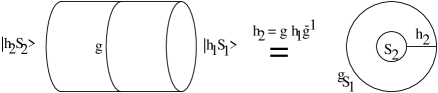
Figure 1: The dual descriptions of the cylinder amplitude. In the closed string picture the states are prepared in the twisted sectors $h_{1,2}$ and the operator $g$ is inserted in the propagator. In the open string picture $g$ identifies the sector of the open string theory and $h_{2}$ gets inserted in the propagator.

Using $P^{\dagger}P=P$ we can write the closed string propagator as

$$\langle\!\langle\,c_{2};S_{2}\,|e^{-\frac{2\pi}{l}H}|\,c_{1};S_{1}\,\rangle\!\rangle=$$

$$\quad=\frac{1}{|\Gamma_{S_{1}}||\Gamma_{S_{2}}|}\sum_{g\in\Gamma}\sum_{\begin{subarray}{c}h_{2}\in\Gamma_{S_{2}}\\ h_{1}\in\Gamma_{S_{1}}\end{subarray}}\langle\!\langle\,h_{2};S_{2},+\,|c_{2}^{*}(h_{2})g\varepsilon(h_{1},g)c_{1}(h_{1})e^{-\frac{2\pi}{l}H}|\,h_{1};S_{1},+\,\rangle\!\rangle$$

$$\quad=\frac{1}{|\Gamma_{S_{1}}||\Gamma_{S_{2}}|}\sum_{\begin{subarray}{c}[f]\in\Gamma_{S_{2}}\backslash\Gamma/\Gamma_{S_{1}}\\ k_{1}\in\Gamma_{S_{1}}\\ k_{2}\in\Gamma_{S_{2}}\end{subarray}}\frac{1}{|\Gamma_{S_{2}}\cap\Gamma_{\,{}^{f}S_{1}}|}\times$$

$$\qquad\qquad\times\sum_{\begin{subarray}{c}h_{2}\in\Gamma_{S_{2}}\\ h_{1}\in\Gamma_{S_{1}}\end{subarray}}\langle\!\langle\,h_{2};S_{2},+\,|c_{2}^{*}(h_{2})k_{2}^{-1}fk_{1}\varepsilon(h_{1},k_{2}^{-1}fk_{1})c_{1}(h_{1})e^{-\frac{2\pi}{l}H}|\,h_{1};S_{1},+\,\rangle\!\rangle\,.$$ (28)

Here we wrote $$g=k_{2}^{-1}fk_{1} k_{i}\in\Gamma_{S_{i}} f \Gamma_{S_{2}}\backslash\Gamma/\Gamma_{S_{1}} \Gamma_{\,{}^{f}S_{1}}\cap\Gamma_{S_{2}} k_{2}h_{2}k_{2}^{-1}\longrightarrow h_{2} k_{1}fh_{1}f^{-1}k_{1}^{-1}\longrightarrow h_{2}$$ with and an arbitrary representative of the coset and we compensated for the overcounting by dividing by the order of . After the change of variables and and using (26) we obtain

$$\langle\!\langle\,c_{2};S_{2}\,|e^{-\frac{2\pi}{l}H}|\,c_{1};S_{1}\,\rangle\!\rangle=$$

$$\quad=\frac{1}{|\Gamma_{S_{1}}||\Gamma_{S_{2}}|}\sum_{\begin{subarray}{c}[f]\in\Gamma_{S_{2}}\backslash\Gamma/\Gamma_{S_{1}}\\ k_{1}\in\Gamma_{S_{1}}\\ k_{2}\in\Gamma_{S_{2}}\end{subarray}}\frac{1}{|\Gamma_{S_{2}}\cap\Gamma_{\,{}^{f}S_{1}}|}\times$$

$$\qquad\times\sum_{\begin{subarray}{c}h_{2}\in\Gamma_{S_{2}}\\ h_{1}\in\Gamma_{\,{}^{f}S_{1}}\end{subarray}}c_{2}^{*}(k_{2}^{-1}h_{2}k_{2})\varepsilon(k_{1}^{-1}f^{-1}h_{1}fk_{1},k_{2}^{-1}fk_{1})c_{1}(k_{1}^{-1}f^{-1}h_{1}fk_{1})\phi(h_{1},f)\times$$

$$\qquad\times\langle\!\langle\,h_{2};S_{2},+\,|e^{-\frac{2\pi}{l}H}|\,h_{1};\,^{f}S_{1},\,^{f}+\,\rangle\!\rangle\,.$$ (29)

To proceed we need to express the general closed string scalar product in terms of an open string trace:

$$\langle\!\langle\,h_{2};S_{2},\eta_{2}\,|e^{-\frac{2\pi}{l}H}|\,h_{1},S_{1},\eta_{1}\,\rangle\!\rangle =\delta_{h_{1}h_{2}}\mbox{Tr}_{\begin{subarray}{c}S_{1}\eta_{1}\\ S_{2}(-\eta_{2})\end{subarray}}(h_{1}e^{-\pi lH_{o}})\,,$$

where by $\mbox{Tr}_{\begin{subarray}{c}S_{1}\eta_{1}\\ S_{2}\eta_{2}\end{subarray}}$ we mean the trace over the open string Hilbert space with boundary conditions $S_{i=1,2},\eta_{i=1,2}$ at the two ends of the worldsheet. As discussed, the above boundary states have a phase ambiguity which however drops out in expressions involving the sandwiched vectors. A priori there could be an ambiguity in the action of $h_{1}$ in the open string spectrum but since the left hand side of the above equation is completely well-defined, it defines $h_{1}$. This formula follows from the fact that the path integral over the worldsheet with boundaries can be calculated in two channels. Note that the bra in the propagator satisfies the conjugate gluing condition which is why the sign of $\eta_{2}$ is reversed. Also note that the untwisted closed sector, $h_{1}=h_{2}=1$ is the NSNS sector.

Going back to (29) we can now express the closed string propagator in terms of open string traces. Using (27) and (2) the coefficient in the sum simplifies for $h=h_{1}=h_{2}$ as

$$c_{2}^{*}(k_{2}^{-1}hk_{2})\varepsilon(k_{1}^{-1}f^{-1}hfk_{1},k_{2}^{-1}fk_{1})c_{1}(k_{1}^{-1}f^{-1}hfk_{1})=c_{2}^{*}(h)c_{1}(f^{-1}hf)\varepsilon(f^{-1}hf,f)\,,$$

and as $k_{1,2}$ drop out of the summand this leads to

$$\langle\!\langle\,c_{2};S_{2}\,|e^{-\frac{2\pi}{l}H}|\,c_{1};S_{1}\,\rangle\!\rangle=\sum_{[f]\in\Gamma_{S_{2}}\backslash\Gamma/\Gamma_{S_{1}}}\frac{1}{|\Gamma_{S_{2}}\cap\Gamma_{\,{}^{f}S_{1}}|}\times\\ \times\sum_{h\in\Gamma_{S_{2}}\cap\Gamma_{\,{}^{f}S_{1}}}c_{2}^{*}(h)\varepsilon(f^{-1}hf,f)c_{1}(f^{-1}hf)\phi(h,f)\mbox{Tr}_{\begin{subarray}{c}\,{}^{f}S_{1},\,^{f}+\\ S_{2},-\end{subarray}}(he^{-\pi lH_{o}})\,.$$ (30)

Having derived the final formula for the partition function in the open string channel we will turn to a discussion of it’s consequences.

The sum over $[f]\in\Gamma_{S_{2}}\backslash\Gamma/\Gamma_{S_{1}}$ is a sum over the different sectors of the open string while the sum over $h\in\Gamma_{S_{2}}\cap\Gamma_{\,{}^{f}S_{1}}$ projects out some of the states in the sector twisted by $f$. The physical condition is that the an integer number of states should be picked out, or more precisely that the projection selects every irreducible representation a nonnegative number of times. In general such a projector has the form

$$P=\frac{1}{|G|}\sum_{g\in G}\chi(g)g\,,$$

where $\chi$ is a character of the group $G$, i.e. $\chi(g)=\mbox{Tr}_{R}(g)$ for some representation $R$. There is one more issue to understand, namely the overall sign that a sector appears with in the partition function. This is the standard partition function of string theory which – from the D-brane worldvolume’s point of view – has an $(-1)^{F}_{worldvolume}$ inserted. In other words worldvolume bosons count positively and worldvolume fermions count negatively. In the above sum over open string sectors the bosons come from the NS sector, which has antiperiodic boundary conditions on the worldsheet fermions. This happens for $f\in\Gamma_{sym}$ since ${}^{f}+=+$ for $f\in\Gamma_{sym}$. Similarly the states are worldvolume fermions in the R sector. The R sector is for asymmetric $f$, i.e. of the form $f=(-1)^{F_{L}}f_{0}$ for $f_{0}\in\Gamma_{sym}$. We also note that the constant $|\Gamma_{S_{2}}\cap\Gamma_{\,{}^{f}S_{1}}|$ in (30) is exactly the order of the group which is being summed over.

Combining everything we are ready to state the conditions on the coefficients in (30). For worldvolume bosons, $f\in\Gamma_{sym}$

$$c_{2}^{*}(h)c_{1}(f^{-1}hf)\varepsilon(f^{-1}hf,f)\,,$$

is a character of $\Gamma_{S_{2}}\cap\Gamma_{\,{}^{f}S_{1}}$. Here we used that $\phi(h,f)=1$ for $f$ symmetric.

For worldvolume fermions, $f=(-1)^{F_{L}}f_{0}$, $f_{0}\in\Gamma_{sym}$

$$c_{2}^{*}(h)c_{1}(f^{-1}hf)\varepsilon(f^{-1}hf,f)\phi(h,(-1)^{F_{L}})=\\ =c_{2}^{*}(h)c_{1}(f_{0}^{-1}hf_{0})\varepsilon(f_{0}^{-1}hf_{0},f_{0})\varepsilon(h,(-1)^{F_{L}})\phi(h,(-1)^{F_{L}})\,,$$ (31)

is minus a character of $\Gamma_{S_{2}}\cap\Gamma_{\,{}^{f}S_{1}}$. Here we used that $\phi(h,f)=\phi(h,(-1)^{F_{L}}f_{0})=\phi(h,(-1)^{F_{L}})$. It is minus a character because worldvolume fermions are counted with a minus sign.

Let us discuss the compatibility of these two conditions. They are compatible if and only if $h\rightarrow\phi(h,(-1)^{F_{L}})$ is minus a character. Here we used that $\varepsilon(h,(-1)^{F_{L}})$ is a character which has an inverse character. Since we believe in the consistency of the theory we thus conclude that $\phi(h,(-1)^{F_{L}})$ is minus a character. So far the only knowledge we had about $\phi(h,(-1)^{F_{L}})$ was that it takes the values $1$ or $-1$, it was a class function and that $\phi(1,(-1)^{F_{L}})=-1$. These facts agree nicely with the conclusion that it is minus a character. Later we will have more to say about it.

We thus conclude that the physical D-brane states are characterized by a gluing condition $S$, a function $c(h)$, $h\in\Gamma_{S}$ which satisfies

$$c(khk^{-1})=c(h)\varepsilon(h,k)\qquad\qquad\qquad h,k\in\Gamma_{S}\,,$$ (32)

and for any two D-branes characterized by $$S_{1},S_{2} c_{1},c_{2}$$ and ,

$$c_{2}^{*}(h)c_{1}(f^{-1}hf)\varepsilon(f^{-1}hf,f)\,,$$ (33)

is a character of $\Gamma_{S_{2}}\cap\Gamma_{\,{}^{f}S_{1}}$ for any $f\in\Gamma_{sym}$. The set of allowed states constitute a cone, i.e. it is additive and an allowed state can be multiplied by a nonnegative integer.

In the next two sections we will discuss what the allowed set of D-brane states are. Starting with the case without discrete torsion followed by the case with discrete torsion.

4.1 No discrete torsion

In case of no discrete torsion the coefficients $c$ are class functions. The physical condition implies that the function $c_{2}^{*}(h)c_{1}(f^{-1}hf)$ is a character of $\Gamma_{S_{2}}\cap\Gamma_{\,{}^{f}S_{1}}$ for any $f\in\Gamma_{sym}$. In order to see what this means for the individual functions $c(h)$ we shall now consider specific examples:

D-instantons

First let’s look at the product of boundary states with $S_{1}=S_{2}=1\mbox{l}$. These gluing conditions are left invariant by $\Gamma_{S_{1}}=\Gamma_{S_{2}}=\Gamma_{sym}$. The only $f$ to consider is $f=1$. and $\Gamma_{\,{}^{f}S_{1}}=\Gamma_{sym}$. We thus need $c_{2}^{*}(h)c_{1}(h)$ to be a character of $\Gamma_{sym}$. This is satisfied if the $c(h)$ are taken to be the characters of $\Gamma_{sym}$. This is exactly our assumption through the paper that all the fractional D-instantons exist. We remember that characters are of the form $c(h)=Tr_{R}(h)$ for some representation $R$ of $\Gamma_{sym}$. Of these the elementary ones correspond to the irreducible representations.

D-instanton with another boundary state

We now let $S_{2}$ be generic while restricting $S_{1}=1\mbox{l}$. The only $f$ to check is again $f=1$. Again $\Gamma_{S_{1}}=\Gamma_{sym}$ so the physical condition is that $c_{2}^{*}(h)c_{1}(h)$ is a character of $\Gamma_{S_{2}}$. Since we can especially choose $c_{1}(h)=1$ it implies that $c_{2}^{*}(h)$ and hence $c_{2}(h)$ is a character. It is natural to call those D-branes elementary for which this representation is irreducible.

Two arbitrary D-branes

Having found that consistent interaction with the elementary D-instanton requires the coefficients of any boundary state to be characters, we now show that the interaction of any two of these is consistent with open-closed duality. To this end note that $f\in\Gamma_{sym}$ generates a group homomorphism:

$$f :\Gamma_{\,{}^{f}S_{1}}\longmapsto\Gamma_{S_{1}} f :h\longmapsto f^{-1}hf\,,$$

implying that if $c_{1}$ is a character of $\Gamma_{S_{1}}$ then $h\mapsto c_{1}(f^{-1}hf)$ is a character of $\Gamma_{\,{}^{f}S_{1}}$. Furthermore when a character is restricted to a subgroup then it becomes a character of that subgroup so that both $h\mapsto c_{2}(h)$ and $h\mapsto c_{1}(f^{-1}hf)$ are characters of $\Gamma_{S_{2}}\cap\Gamma_{\,{}^{f}S_{1}}$. Since the product of characters is again a character, the condition for the consistency with open-closed duality is satisfied.

4.2 Discrete torsion

Now we turn to the general case. It was conjectured by Douglas and Fiol [8, 9] that in this case the D-branes are classified by projective representations. Remembering the connection between discrete torsion and projective representations it is a natural generalization of the ordinary case. Let us show that this indeed works. For a given gluing condition $S$ we need a function $c(h)$ defined on $\Gamma_{S}$. Let $\gamma:\Gamma_{S}\rightarrow GL(n,{\mathbb{C}})$ be a projective representation of $\Gamma_{S}$ corresponding to the given $\varepsilon$. This means that $\gamma$ satisfies (6) and $c(g,h)$ is related to $\varepsilon$ by (10). Let us now define

$$c(h) =\mbox{Tr}(\gamma(h)) h\in\Gamma_{S}\,.$$ (34)

Our claim is now that this set of coefficients $c$ will span the set of physical states. We have to check two conditions. One is the condition (32) and the other is the physical condition (33). We first prove (32):

$$c(khk^{-1}) =\mbox{Tr}(\gamma(khk^{-1})=\frac{c(k^{-1},k)c(h,1)}{c(kh,k^{-1})c(k,h)}\mbox{Tr}(\gamma(h))\,.$$

Here we used (6), the cyclicity of the trace and (6) again. Now substitute the definition of $$\varepsilon$$ and apply (6) once more:

$$c(khk^{-1}) =\varepsilon(h,k)c(h)\frac{c(k^{-1},k)c(h,1)}{c(kh,k^{-1})c(khk^{-1},k)}=\varepsilon(h,k)c(h)\frac{c(h,1)}{c(kh,1)}=\varepsilon(h,k)c(h)\,,$$

exactly as desired. The physical condition (33) is a bit harder. With notation as above we need to show that $\varepsilon(f^{-1}hf,f)c_{1}(f^{-1}hf)c_{2}^{*}(h)$ is a character. We have

$$\varepsilon(f^{-1}hf,f)c_{1}(f^{-1}hf)c_{2}^{*}(h) =\varepsilon(f^{-1}hf,f)\mbox{Tr}(\gamma_{1}(f^{-1}hf))\mbox{Tr}(\gamma_{2}(h))^{*}$$

$$=\mbox{Tr}(\varepsilon(f^{-1}hf,f)\gamma_{1}(f^{-1}hf)\otimes\gamma^{*}_{2}(h))\,,$$

where the last trace is over the tensor product representation. This is a character of $\Gamma_{S_{2}}\cap\Gamma_{\,{}^{f}S_{1}}$ if $R(h)=\varepsilon(f^{-1}hf,f)\gamma_{1}(f^{-1}hf)\otimes\gamma^{*}_{2}(h)$ is a proper representation, i.e. not projective. It indeed is as we will now show.

$$R(g)R(h) =\varepsilon(f^{-1}gf,f)\varepsilon(f^{-1}hf,f)(\gamma_{1}(f^{-1}gf)\gamma_{1}(f^{-1}hf)\otimes(\gamma^{*}_{2}(g)\gamma^{*}_{2}(h))$$

$$=\frac{\varepsilon(f^{-1}gf,f)\varepsilon(f^{-1}hf,f)}{\varepsilon(f^{-1}ghf,f)}\frac{c(f^{-1}gf,f^{-1}hf)}{c(g,h)}R(gh)\,.$$

We need to calculate the coefficient of $R(gh)$ and show that it is one. Plugging in the definition of $\varepsilon$ this coefficient reads as

$$\frac{c(g,f)c(h,f)c(f^{-1}gf,f^{-1}hf)c(f,f^{-1}gh,f)}{c(f,f^{-1}gf)c(f,f^{-1}hf)c(g,h)c(f,gh)} =\frac{c(g,f)c(h,f)c(f,f^{-1}gf)c(gf,f^{-1}hf)}{c(f,f^{-1}gf)c(f,f^{-1}hf)c(g,hf)c(h,f)}$$

$$=\frac{c(g,hf)c(f,f^{-1}hf)}{c(f,f^{-1}hf)c(g,hf)}=1\,.$$

Here we used (7). We thus conclude that $R(g)R(h)=R(gh)$ as claimed. Since $R$ is a representation its trace is a character. We have thus proven that the physical condition is satisfied for the traces of the projective representations. Of course, the case without discrete torsion is a special case of this.

4.3 Determination of $\phi(h,(-1)^{F_{L}})$

We see that the spectrum of open string states depends on the function $\phi(h,(-1)^{F_{L}})$, with $h\in\Gamma_{sym}$. Is there any way to determine $\phi(h,(-1)^{F_{L}})$ ? What we know about $\phi(h,(-1)^{F_{L}})$ is that it takes the value $\pm 1$ and it is minus a character. It actually turns out that it could be any character and the various choices differ by discrete torsion. To see that, write the orbifold group as $\Gamma=\{1,(-1)^{F_{L}}\}\times\Gamma_{sym}$ and let $\chi(h)$ be any character of $\Gamma_{sym}$ that takes the values $\pm 1$. This particularly implies that $\chi=\chi^{-1}$. Any element of $\Gamma$ can be written $((-1)^{F_{L}})^{n}h$, where $n\in Z_{2}$ and $h\in\Gamma_{sym}$. Now define a discrete torsion as follows

$$\varepsilon(((-1)^{F_{L}})^{n_{1}}h_{1},((-1)^{F_{L}})^{n_{2}}h_{2})=\chi(h_{2})^{n_{1}}\chi(h_{1})^{n_{2}}\,.$$

It is easily seen that it satisfies the conditions (2) and (5). Here it is essential that $\chi=\chi^{-1}$. Now introduction of this discrete torsion changes $\phi$ to

$$\phi^{\prime}(h,k)=\phi(h,k)\varepsilon(h,k)\,.$$

Recall that $\phi(h,k)$ is defined for $h\in\Gamma_{sym}$ and $k\in\Gamma$. For $k\in\Gamma_{sym}$ we still have

$$\phi^{\prime}(h,k)=1\,,$$

and

$$\phi^{\prime}(h,(-1)^{F_{L}})=\phi(h,(-1)^{F_{L}})\varepsilon(h,(-1)^{F_{L}})=\phi(h,(-1)^{F_{L}})\chi(h)\,.$$

We thus see that $\phi^{\prime}$ is still minus a character and it can be any one taking the values $\pm 1$. Especially we could choose $\chi(h)$ to be $-\phi(h,(-1)^{F_{L}})$ making $\phi^{\prime}(h,(-1)^{F_{L}})=-1$.

5 Conclusion

We have generalized the connection between the phases $\varepsilon$, and projective representations to nonabelian groups (10). We found explicit formulas for the boundary states with gluing conditions in $U(4)$. Open-closed string duality is satisfied by boundary states given as projective characters. It would be possible to study other D-branes in these theories without too much trouble, since the orbifold action has been fixed, for example one could study the unstable branes which correspond to $S\in O(8)$ with $\det(S)=-1$.

References

• [1] C. Vafa, Modular invariance and discrete torsion on orbifolds, Nucl. Phys. B273 (1986) 592.
• [2] C. Vafa and E. Witten, On orbifolds with discrete torsion, J. Geom. Phys. 15 (1995) 189–214, [hep-th/9409188].
• [3] J. Callan, Curtis G., C. Lovelace, C. R. Nappi, and S. A. Yost, Loop corrections to superstring equations of motion, Nucl. Phys. B308 (1988) 221.
• [4] J. Polchinski and Y. Cai, Consistency of open superstring theories, Nucl. Phys. B296 (1988) 91.
• [5] P. Di Vecchia and A. Liccardo, D branes in string theory. I, hep-th/9912161.
• [6] P. Di Vecchia and A. Liccardo, D-branes in string theory. II, hep-th/9912275.
• [7] A. Recknagel and V. Schomerus, D-branes in Gepner models, Nucl. Phys. B531 (1998) 185–225, [hep-th/9712186].
• [8] M. R. Douglas, D-branes and discrete torsion, hep-th/9807235.
• [9] M. R. Douglas and B. Fiol, D-branes and discrete torsion. ii, hep-th/9903031.
• [10] S. Mukhopadhyay and K. Ray, D-branes on fourfolds with discrete torsion, Nucl. Phys. B576 (2000) 152–176, [hep-th/9909107].
• [11] D. Berenstein and R. G. Leigh, Discrete torsion, AdS/CFT and duality, JHEP 01 (2000) 038, [hep-th/0001055].
• [12] J. Gomis, D-branes on orbifolds with discrete torsion and topological obstruction, JHEP 05 (2000) 006, [hep-th/0001200].
• [13] M. Klein and R. Rabadan, Orientifolds with discrete torsion, JHEP 07 (2000) 040, [hep-th/0002103].
• [14] P. S. Aspinwall and M. R. Plesser, D-branes, discrete torsion and the McKay correspondence, JHEP 02 (2001) 009, [hep-th/0009042].
• [15] P. S. Aspinwall, A note on the equivalence of Vafa’s and Douglas’s picture of discrete torsion, JHEP 12 (2000) 029, [hep-th/0009045].
• [16] B. Feng, A. Hanany, Y.-H. He, and N. Prezas, Discrete torsion, covering groups and quiver diagrams, JHEP 04 (2001) 037, [hep-th/0011192].
• [17] E. R. Sharpe, Discrete torsion, hep-th/0008154.
• [18] M. Gutperle, Non-BPS D-branes and enhanced symmetry in an asymmetric orbifold, JHEP 08 (2000) 036, [hep-th/0007126].
• [19] I. Brunner, A. Rajaraman, and M. Rozali, D-branes on asymmetric orbifolds, Nucl. Phys. B558 (1999) 205–215, [hep-th/9905024].
• [20] D.-E. Diaconescu and J. Gomis, Fractional branes and boundary states in orbifold theories, JHEP 10 (2000) 001, [hep-th/9906242].
• [21] D.-E. Diaconescu and M. R. Douglas, D-branes on stringy Calabi-Yau manifolds, hep-th/0006224.
• [22] M. Billo, B. Craps, and F. Roose, Orbifold boundary states from Cardy’s condition, JHEP 01 (2001) 038, [hep-th/0011060].
• [23] M. R. Gaberdiel and J. Stefanski, Bogdan, Dirichlet branes on orbifolds, Nucl. Phys. B578 (2000) 58–84, [hep-th/9910109].
• [24] M. R. Gaberdiel, Discrete torsion orbifolds and D-branes, JHEP 11 (2000) 026, [hep-th/0008230].
• [25] B. Craps and M. R. Gaberdiel, Discrete torsion orbifolds and D-branes. II, JHEP 04 (2001) 013, [hep-th/0101143].
• [26] M. R. Douglas and G. Moore, D-branes, quivers, and ALE instantons, hep-th/9603167.
• [27] O. Bergman and M. R. Gaberdiel, On the consistency of orbifolds, Phys. Lett. B481 (2000) 379–385, [hep-th/0001130].
• [28] J. L. Cardy, Boundary conditions, fusion rules and the Verlinde formula, Nucl. Phys. B324 (1989) 581.