N=2 Supersymmetry and de Sitter space

Abstract:

We present a (unique?) possibility of de Sitter solution in the framework of N=2 supersymmetry (hypersymmetry). We show that a model with a vector and a charged hypermultiplet has a hybrid inflation type potential. It leads to a slow-roll regime in de Sitter type background with all supersymmetries broken spontaneously. Beyond the bifurcation point the waterfall stage abruptly brings the system into a ground state with 2 unbroken supersymmetries. De Sitter stage exists under condition that the superconformal $SU(2,2|2)$ symmetry of the model is softly broken down to N=2 supersymmetry by the vev of the Killing prepotential triplet $P^{r}$. This hybrid hypersymmetry model may describe P-term inflation and/or acceleration of the universe at the present epoch.

1 Introduction

Current cosmological observations indicate that there could be a stage of a rapid accelerated expansion (inflation) in the very early universe [1]. Such a stage could start immediately after the big bang and it could last as long as $10^{-35}$ seconds (in the simplest inflationary models). Moreover, observations indicate that few billion years after the big bang (half-way to the present epoch) the universe entered a second stage of accelerated expansion. The rate of acceleration (the Hubble constant) now is approximately 60 orders of magnitude smaller than during the stage of inflation in the early universe. For a discussion of the observations and their theoretical interpretation see e.g. [2].

Usually it is assumed that the energy-momentum tensor during inflation is dominated by potential energy density of a scalar field, $T_{\mu\nu}\approx g_{\mu\nu}V(\phi)$ with $V>0$. This condition requires that the scalar field moves very slowly, $\dot{\phi}^{2}/2\ll V(\phi)$ [3]. The limiting case $\dot{\phi}=0$ corresponds to de Sitter space with a positive cosmological constant. Similarly, current cosmological acceleration can be explained either by a positive vacuum energy $V$ (cosmological constant) or some kind of slowly rolling scalar field in a near de Sitter background with $\dot{\phi}^{2}/2\ll V(\phi)$ [4].

For the sake of the argument, let us assume that inflation and acceleration of the universe will be supported by future experiments and moreover, the supersymmetric particles will be detected and supersymmetry confirmed. What kind of theories can be used to explain such experiments?

The relation between supersymmetry, supergravity and positive cosmological constant was considered as problematic for a long time [5]-[7]. It has been recognized long ago that in extended supersymmetric theories de Sitter solutions are unstable solutions with broken supersymmetry[8, 9].

Recently it was pointed out that it may not be easy to describe de Sitter space and accelerating universe in M/string theory [10]-[16]. It was particularly stressed by Witten in [14] that no clear-cut way to get de Sitter space from M/string theory is visible. Very recent discussion of these issues can be found in [17, 18, 19].

The new angle from which we would like to look at the old issue is: how unstable is de Sitter space in supersymmetric theories? When can this instability be used in the cosmological context? There are few instances in N=8 and N=4 gauged supergravities related to M/string theory, where de Sitter classical solutions have been found in the past. We shall discuss them in a separate publication [20].

Theories of N=1 supergravity coupled with N=1 matter have an opposite problem. There is an unlimited number of possibilities to find stable de Sitter solutions. The choice of the Kähler potential $K(z,\bar{z})$, the holomorphic superpotential $W(z)$ and D-terms allows various type of potentials with de Sitter vacua. There is no clear preference for one or another choice.

N=2 supersymmetry and N=2 supergravity have not attracted much attention in this respect, to the best of our knowledge . The purpose of this note is to show that a very interesting and rather unique possibility opens up here. We will start with a global $SU(2,2|2)$-superconformal gauge theory which hopefully may be related, via Maldacena conjecture, to string theory compactified on $ADS_{5}\times M^{5}$-space, where $M^{5}$ is some supersymmetry breaking manifold. The model we will study is a well known N=2 QED with one vector multiplet and one charged hypermultiplet. Presumably, it is a part of a more general theory, but the main new features of the cosmological scenario develop in this sector. We add the FI term $\xi$ equal to $\sqrt{2\Lambda}$ where $\Lambda$ is a desirable value of the cosmological constant. This will explicitly break the superconformal symmetry but N=2 supersymmetry will be intact. The theory can be easily coupled consistently to N=1 supergravity; the coupling to N=2 supergravity may face some topological obstructions for non-vanishing constant $\xi$.

We find that the potential of our N=2 model is of the type used in hybrid inflation [22] with de Sitter stage and a waterfall stage. The analogous hybrid potentials were used in F-term inflation [23, 24] and D-term inflation [25, 26, 27], see [28] for a review. Even though the N=2 theory differs substantially from the one used in F-term inflation, in the simplest case of one hypermultiplet our inflationary potential at the classical level exactly coincides with the F-term potential of [24]. It also coincides with the D-term potential of N=1 theory [26] under condition that the gauge coupling $g$ is related to the Yukawa coupling $\lambda$ as follows:

$$\lambda^{2}=2g^{2}\ .$$

The potential depends on vev’s of at least 3 scalar fields (or more), one scalar from the vector multiplet and two from the hypermultiplet.

The mechanism of hybrid inflation may apply not only to early universe and inflation era, but also to the present stage of the accelerating universe (for a different set of fields and parameters). For the early universe inflation in this scenario $\sqrt{\xi\over g}\sim 10^{-2}M_{P}$ with the relevant scale $10^{-30}$ cm but for the present cosmological constant $\sqrt{\xi}\sim 10^{-30}M_{P}$ with the length scale of the order of $10^{-2}$ cm. There will be a long slow change of an ‘inflaton field’ in the near de Sitter space (the space with $T_{\mu\nu}\approx g_{\mu\nu}V$) with broken susy. At the critical point where the vev of the inflaton will reach the value $\sqrt{\xi\over g}$, the potential will switch into the waterfall stage and very fast the ground state with 2 unbroken supersymmetries and vanishing cosmological constant will be reached.

The fundamental role in this cosmological scenario is played by the non-vanishing vev of the third component of the triplet of the Killing prepotentials $P^{r}$ of N=2 theory with special and hyper-Kähler geometry. (In a simplest case this triplet is an auxiliary field of the N=2 vector multiplet). Since inflation and acceleration of the universe in this model appear due to the $P$-term in N=2 supersymmetry, we will call it $P$-term inflation.

This model have several different advantages over the models based on N=1 supersymmetry. First of all, it is much more restrictive than in the more familiar cases of F-term and/or D-term inflation, where one can choose many different superpotentials without a clear guiding principle. In the N=2 theory one does not have this freedom. As a reward, one can show that all non-gravitational quantum corrections in this theory starting from the second loop are finite [30].

The basis of this model is the $SU(2,2|2)$-superconformal symmetry of the gauge theory which may live at the boundary of the $ADS_{5}$ space related to string theory. In this way one may try to connect both inflation and accelerating universe to string theory.

The slow de Sitter type evolution in this model is not eternal. After passing the critical point the Minkowski ground state is naturally reached where one of the hypermultiplet scalars acquires a vev $\sqrt{2\xi\over g}$ and the unbroken N=2 supersymmetry is restored. At this ground state a vector multiplet ‘eats’ a hypermultiplet and transforms into one massive N=2 vector multiplet, which is a super-Higgs effect in N=2 theories. All fields have the same mass $m^{2}=2g\xi$. This overcomes the problem of eternal quintessence pointed out for one scalar field in supersymmetric theories in [15] since in our case the system does relax into a zero-energy supersymmetric vacuum.

2 De Sitter solutions in N=1 supergravity

Before discussion of coupling to supergravity of our N=2 model, let us make a short overview of de Sitter solutions in N=1 supergravity. We will point out necessary and sufficient conditions for N=1 supergravity to have a de Sitter solution.

The well known potential depends on Kähler potential $K(z,\bar{z})$, on holomorphic superpotential $W(z)$ and on a holomorphic function $f_{\alpha\beta}(z)$ in kinetic terms for vector multiplets [31]:

$$V=V_{F}+V_{D}=e^{K\over M_{P}^{2}}\left[({\cal D}^{i}W)K^{-1}{}_{i}{}^{j}({\cal D}_{j}W^{*})-3{WW^{*}\over M_{P}^{2}})\right]+{1\over 2}(\rm Re\,f_{\alpha\beta})D^{\alpha}D^{\beta}\ .$$ (1)

The potential is not positive definite, the negative contribution is proportional to the square of the gravitino mass,

$$M_{\rm gravitino}={W\over M^{2}_{P}}e^{K\over 2M_{P}^{2}}\ .$$

To find a de Sitter solution one has to find some constant values of all scalars at which the potential has an extremum with

$$3|W|^{2}<|F|^{2}+{1\over 2}|D|^{2}e^{-{K\over M_{P}^{2}}}\ .$$ (2)

where $|F|^{2}\equiv({\cal D}^{i}W)K^{-1}{}_{i}{}^{j}({\cal D}_{j}W^{*})$. Clearly, any solution with vanishing or very small superpotential $W$ at the critical point and with non-vanishing F-term, derivative of the superpotential, and/or non-vanishing D-term will give a de Sitter solution. There are many ways to get it.

Consider an example:

$$K=zz^{*}+yy^{*}\ ,W=(z^{2}+a)y\ .$$ (3)

The critical point of the potential at $z=y=0$ gives a de Sitter solution. The value of the potential at this critical point is

$$V_{0}=a^{2}\ .$$ (4)

There are many known examples with vanishing chiral multiplets contribution, in all such cases D-terms will give a positive cosmological constant. Thus N=1 supergravity needs some motivation from any version of a more fundamental theory like M/string theory about the choice of ${\cal G}$ and relevant physics.

3 Hybrid hypersymmetry model

To reveal the essential features of hypersymmetry in cosmology we will use a simple N=2 model suggested by Salam and Strathdee [33] and Fayet [34] (SSF model). The reader familiar with Witten-Seiberg paper [35] may find it easy to recall the model as a warm-up example there: QED with matter, i.e. an abelian gauge theory with N=2 supersymmetry and charged matter hypermultiplets. We will first study the version of the theory with massless hypermultiplets and explain the massive case later. In what follows we consider one hypermultiplet, more general case will have analogous important features and, perhaps, more. The supersymmetric ground state of this model is well known, the existence of the local valley with positive potential was not noticed before in this N=2 model.

3.1 $SU(2,2|2)$ superconformal part of the model

In terms of N=1 superfields the superconformal part of the model is rather simple, in notation of [34] it is:

$${\cal L}={\cal L}_{0}+[S^{*}e^{2gV}S+T^{*}e^{-2gV}T+N^{*}N]_{D}+[4gT^{*}SN]_{F}\ .$$ (5)

Here ${\cal L}_{0}$ is the kinetic term for the $U(1)$ gauge multiplet, $N$ is the neutral chiral supermultiplet whereas $S$ and $T$ are charged chiral superfields of the opposite charge. There is only one coupling constant, both for gauge coupling and for Yukawa coupling.

It will be useful for our purpose to present this theory in terms of component fields with off-shell rigid N=2 supersymmetry, following [32, 37].

We have an abelian N=2 gauge multiplet which belongs to a representations of rigid $SU(2)$, the antisymmetric tensor $\varepsilon_{AB}$, $A,B=1,2$, is used to raise and lower the $SU(2)$ indices. The multiplet consists of two scalars $A$ and $B$, a vector $A_{\mu}$, (all singlets in $SU(2)$), a spin-1/2 doublet $\lambda^{A}=\varepsilon^{AB}\gamma_{5}C\bar{\lambda}_{B}^{T}$ (gaugino) and an auxiliary field $P^{r}$, triplet in $SU(2)$. This simple model is a particular case of the general setting of N=2 gauge theories and gauged supergravity where the triplet of Killing prepotentials $P^{r}$ plays an important role in special geometry and in hyper-Kähler (quaternionic for supergravity) manifolds.

A hypermultiplet, N=2 matter multiplet has two complex scalar fields forming a doublet under $SU(2)$, $\Phi^{A}$ and $\Phi_{A}=(\Phi^{A})^{*}$ and a spin 1/2 field $\psi$, singlet under $SU(2)$ (hyperino). There is also a doublet of dimension 2 auxiliary fields, $F^{A}$ with $F_{A}=(F^{A})^{*}$ . The superconformal action is

$${\cal L}_{s.c.} = {1\over 2}[(\partial_{\mu}A)^{2}+(\partial_{\mu}B)^{2}]+{i\over 2}\,\bar{\lambda}_{A}\not\!{\partial}\lambda^{A}-{1\over 4}F_{\mu\nu}^{2}+{1\over 2}\vec{P}^{2}$$

$$+ {1\over 2}D_{\mu}\Phi^{A}D^{\mu}\Phi_{A}+i\,\bar{\psi}\not\!{D}\psi+F^{A}F_{A}$$

$$+ ig\Phi^{A}\bar{\lambda}_{A}\psi-ig\bar{\psi}\lambda^{A}\Phi_{A}-g\bar{\psi}(A-\gamma_{5}B)\psi+{g\over 2}\Phi^{A}\vec{\sigma}_{A}{}^{B}\vec{P}\Phi_{B}-{g^{2}\over 2}\Phi^{A}(A^{2}+B^{2})\Phi_{A}\ .$$

The covariant derivatives on the hypers are

$$D_{\mu}\Phi_{A} = \partial_{\mu}\Phi_{A}+igA_{\mu}\Phi_{A}\ ,$$

$$D_{\mu}\Phi^{A} = \partial_{\mu}\Phi^{A}-igA_{\mu}\Phi^{A}\ ,$$

$$D_{\mu}\psi = \partial_{\mu}\psi+igA_{\mu}\psi\ .$$ (7)

The first line in (3.1) is for the vector multiplet, the second one is for the hypermultiplet. Note that all 6 scalars, $f\equiv\{A,B,a_{1},b_{1},a_{2},b_{2}\}$, where $\Phi_{1}=a_{1}+ib_{1}$ and $\Phi_{2}=a_{2}+ib_{2}$ have canonical kinetic terms of the form ${1/2}(\partial f)^{2}$. The third line includes terms which must be added to the action simultaneously with covariantization of derivatives. All term depending on $g$ describe the gauging. When the gauge coupling $g$ is vanishing, the theory is a non-interacting theory of a vector multiplet and a neutral hypermultiplet.

The model has 2 rigid supersymmetries (hypersymmetry) with the Majorana spinors $\varepsilon^{A}=\varepsilon_{AB}\gamma_{5}C\bar{\varepsilon}_{B}^{T}$. The fields of the gauge multiplet transform as follows:

$$\delta A_{\mu} = i\,\bar{\epsilon}_{A}\,\gamma_{\mu}\,\lambda^{A}\,,\qquad\delta A=i\,\bar{\epsilon}_{A}\,\lambda^{A}\,,\qquad\delta B=i\,\bar{\epsilon}_{A}\,\gamma^{5}\,\lambda^{A}\,,$$

$$\delta\lambda^{A} = -\frac{i}{2}\,\sigma^{\mu\nu}\,\epsilon^{A}F_{\mu\nu}-\gamma^{\mu}\,\partial_{\mu}\,(A+\gamma_{5}\,B)\,\epsilon^{A}-i\,\epsilon^{B}\,\vec{\sigma}_{B}{}^{A}\,\vec{P}\,,$$ (8)

$$\delta\vec{P} = \epsilon_{B}\,\vec{\sigma}_{A}{}^{B}\,\gamma^{\mu}\,\partial_{\mu}\lambda^{A}\ .$$

The supersymmetry transformations of the fields of the hypermultiplets are

$$\delta\Phi_{A} = 2\,\bar{\epsilon}_{A}\,\psi\,,\qquad\delta F_{A}=2\,\bar{\epsilon}_{A}\,(\gamma^{\mu}\,D_{\mu}+g(i\,A-i\,\gamma_{5}\,B))\psi-2g\bar{\epsilon}_{B}\,\lambda^{B}\,\Phi_{A},$$

$$\delta\psi = -i\,\epsilon^{\,A}\,F_{A}-i\,\gamma^{\mu}\,D_{\mu}\epsilon^{\,A}\,\Phi_{A}+g(A+\gamma_{5}\,B)\,\epsilon^{\,A}\,\Phi_{A}\ .$$ (9)

Using equations of motion for auxiliary fields,

$$P^{r}=-{g\over 2}\Phi^{A}(\sigma^{r})_{A}{}^{B}\Phi_{B}\ ,\qquad F^{A}=0$$ (10)

we find the potential

$$V_{s.c.}={g^{2}\over 2}[\Phi^{\dagger}\Phi(A^{2}+B^{2})+{1\over 4}(\Phi^{\dagger}\vec{\sigma}\Phi)^{2}]\ ,$$

where $\Phi^{\dagger}\Phi\equiv\Phi^{A}\Phi_{A}=|\Phi_{1}|^{2}+|\Phi_{2}|^{2}\geq 0$. It is also possible to rewrite the potential as follows:

$$V_{s.c.}={g^{2}\over 2}[\Phi^{\dagger}\Phi(A^{2}+B^{2})+{1\over 4}(\Phi^{\dagger}\Phi)^{2}]\ .$$ (11)

The theory has a dilatation symmetry and $U(2)$ symmetry and it is symmetric under the superconformal symmetry $SU(2,2|2)$, see [36, 37]. This adds special conformal and special supersymmetry. The bosonic symmetry $SU(2,2)$ is an isometry of the $adS_{5}$ space which may connect this gauge theory to string theory on the boundary of the $adS_{5}$ space. The general conditions for conformal invariant hypermultiplets theories have been found in [38].

3.2 N=2 supersymmetry after soft breaking of superconformal symmetry

There are two possibilities to break $SU(2,2|2)$ symmetry down to N=2 supersymmetry. The first one is to make a hypermultiplet massive. This is equivalent to a shift of the vev of the $A$ field, a scalar from the vector multiplet and it does not make important changes. A dramatic change in the behaviour of the potential takes place if the N=2 FI terms $\xi^{r}$ are added to the theory (for abelian multiplet only). The N=2 supersymmetry of the action remains intact. The new action is:

$${\cal L}_{N=2}={\cal L}_{s.c.}+P^{r}\xi^{r}\ .$$ (12)

This will change the field equation for $P^{r}$, which will become

$$P^{r}=-{g\over 2}(\Phi^{\dagger}\sigma^{r}\Phi)-\xi^{r}\ .$$ (13)

The potential of our hypersymmetric model becomes equal to

$$V=g^{2}[\Phi^{\dagger}\Phi(A^{2}+B^{2})+{1\over 4}(\Phi^{\dagger}\vec{\sigma}\Phi+{2\over g}\vec{\xi})^{2}]\ .$$ (14)

We chose to have a FI term only in the direction $3$ and to have it positive

$$\xi^{r}=(0,0,\xi)\ ,\qquad\xi>0\ .$$ (15)

We can rewrite it in the form where it is clear that this is a hybrid-type potential [22]-[28]:

$$V_{N=2}={g^{2}\over 2}[(|\Phi_{1}|^{2}+|\Phi_{2}|^{2})|\Phi_{3}|^{2}+|\Phi_{1}|^{2}|\Phi_{2}|^{2}+{1\over 4}(|\Phi_{1}|^{2}-|\Phi_{2}|^{2}+{2\over g}\xi)^{2}]\ ,$$ (16)

where we introduced the notation $\Phi_{3}\equiv A+iB$. At $\xi=0$ the potential is equal to the one of the superconformal theory, as given in (11). The potential of this N=2 supersymmetric theory coincides with the particular case studied before in the cosmological context of the D-term inflation in [26]. There N=1 global susy theory is defined by a superpotential $W=\lambda X\phi_{+}\phi_{-}$ and the chiral multiplets $\phi_{+}$ and $\phi_{-}$ have positive and negative charges under $U(1)$. This potential leads to hybrid inflation [22]. In the previous studies N=1 supersymmetric gauge theory was used, therefore the gauge coupling $g$ and the Yukawa coupling $\lambda$ were not related. For the special case that $\lambda=\sqrt{2}g$ the theory has N=2 supersymmetry [33, 34]. Our notations may be compared with notation in Dvali-Binetruy [26] as follows: $\Phi_{1}=\phi_{+}$ and $\Phi_{2}=\phi_{-}^{*}$ and $\Phi_{3}=X$, $2\xi/g=\xi_{\rm DB}$ and $g=2g_{\rm DB}$. The potential of our N=2 supersymmetric theory coincides also with the F-term inflation N=1 theory, proposed in [24].

3.3 Hybrid hypersymmetry model as an example of generic N=2 gauge theory

It may be quite important to show how this model fits in the general class of rigid N=2 gauge theories [40]. Particularly since it will help to understand a coupling to supergravity. In generic case one defines the rigid special Kähler and hyper-Kähler manifolds and identifies their isometries. The gauging involves covariant derivatives on coordinates of the special Kähler manifold $z_{i},\bar{z}^{i}$ and on coordinates of the hyper-Kähler manifold $q^{u}$:

$$D_{\mu}z_{i} = \partial_{\mu}z_{i}+gA_{\mu}^{I}k_{Ii}\ ,$$

$$D_{\mu}\bar{z}^{i} = \partial_{\mu}\bar{z}^{i}+gA_{\mu}^{I}k_{I}^{i*}\ ,$$

$$D_{\mu}q^{u} = \partial_{\mu}q^{u}+gA_{\mu}k_{I}^{u}\ .$$ (17)

Here $k_{I}^{l}$ are the Killing vectors of rigid special geometry and $k_{I}^{u}$ are Killing vectors of the hyper-Kähler geometry, for each gauge group $I=1,2,\dots,n$. There are $n$ vector multiplets, so that $I=1,\dots,n$. The special Kähler manifold of the rigid type is defined by a holomorphic section $\Omega=(Y^{I},F_{I})$ of a flat bundle, where $Y^{I}(z)$ are special complex coordinates and $F_{I}$ are the derivatives of the prepotential $F(Y)$. A Kähler potential is given by ${\cal K}=i(\bar{Y}^{I}F_{I}-\bar{F}_{J}Y^{J})$. A derivative of the holomorphic section $\Omega$ includes the functions $f^{Ii}$ and $h_{I}^{i}$) which serve to define the period matrix. In presence of hypermultiplets a particular N=2 gauge theory is defined in terms of the triplet of the prepotentials $P^{r}$, $r=1,2,3$. There are various relations between Killing vectors and prepotentials. The gauging leads to most general potentials of N=2 supersymmetric gauge theory:

$$V_{\rm susy}^{N=2}(z,\bar{z},q)=g^{2}(g^{i}{}_{j}k_{Ii}k^{*j}_{J}+4h_{uv}k^{u}_{I}k^{v}_{J}){\bar{Y}}^{I}Y^{J}+g^{i}{}_{j}f^{I}_{i}f^{*jJ}\sum_{r=1}^{r=3}P_{I}^{r}P_{J}^{r}\ .$$ (18)

Here $g^{i}{}_{j}$ is the metric for scalars of the special geometry, and $h_{uv}$ is the metric for the hypers. The potential is non-negative definite.

Our model with one gauge group, $I=1$, gives a particular case of this potential: we have flat metrics $g^{i}{}_{j}$ and $h_{uv}$ and no Killing vectors on special manifolds, so the first term in (18) is absent in our model. The second term in (18) can be easily identified with the first term in our model potential (16) since the Killing vectors are proportional to hypers and $Y,\bar{Y}$ are the scalars from a vector multiplet. The second term in (16) is proportional to $(P^{1})^{2}+(P^{2})^{2}$ and the third term in (16) is proportional to $(P^{3})^{2}$. Together they reproduce the last term in eq. (18). In a more compact form of our potential in eq. (14) we may identify the last terms with the last term in generic N=2 potential in (18).

3.4 Vacua of the hybrid hypersymmetry model

For the vacuum solutions we chose the vanishing vector field and constant values of 3 complex scalar fields $\Phi_{1},\Phi_{2},\Phi_{3}$. The potential (16) has two minima.

1. Non-supersymmetric local minimum with flat directions (de Sitter valley) at some undefined but restricted constant value of the scalar $\Phi_{3}$, all other scalars vanish.

$$\Phi_{1}=\Phi_{2}=0\ ,\qquad|\Phi_{3}|=|\Phi_{3}|_{0}\ ,\qquad P^{3}=-\xi\ ,\qquad V_{0}={1\over 2}\xi^{2}\ .$$ (19)

This is a local minimum of the potential for $|\Phi_{3}|_{0}^{2}>{\xi\over g}$. The curvature of the potential is positive when this restriction is applied

$$M_{1}^{2}=g^{2}|\Phi_{3}|_{0}^{2}+g\xi\ ,\qquad M_{2}^{2}=g^{2}|\Phi_{3}|_{0}^{2}-g\xi\ ,$$ (20)

and there are flat directions like $V_{,33}=0$. The supersymmetry variation of fermions (8), (9) at this vacuum is:

$$\delta\lambda^{1}=-i\xi\varepsilon^{1}\ ,\qquad\delta\lambda^{2}=+i\xi\varepsilon^{2}\ ,\qquad\delta\psi=0\ .$$ (21)

Therefore, as long as $\xi\neq 0$, all supersymmetries are broken. When coupled to gravity, this vacuum corresponds to a de Sitter solution.

2. Supersymmetric global minimum

$$(\Phi_{3})_{\rm susy}=(\Phi_{1})_{\rm susy}=P^{3}_{\rm susy}=0\ ,\qquad|\Phi_{2}|_{\rm susy}=\sqrt{2\xi\over g}\ ,\qquad V_{\rm susy}=0\ .$$ (22)

Short inspection of the supersymmetry transformation of fermions (8), (9) shows that they all vanish:

$$\delta\lambda_{i}=0\ ,\qquad\delta\psi=0\ .$$ (23)

Thus the absolute minimum ground state has both N=2 supersymmetries unbroken and vanishing potential. The full hypersymmetry is unbroken but the $U(1)$ gauge symmetry is spontaneously broken. The massless vector multiplet with one vector field, one complex scalar and one Dirac spinor eats the hypermultiplet with 2 complex scalars and one Dirac spinor. As a result, there is one massive vector multiplet with one massive vector field, two Dirac spinors, one complex scalars and 3 real scalars. All fields have a mass $m^{2}=2g\xi$. This is known in the literature as a hypersymmetric Higgs mechanism. When coupled to gravity, this vacuum corresponds to a solution with zero cosmological constant.

The best way to understand these two critical points of the potential is to look at the 3D plots of the hybrid potential [22]. One of the scalars, $\Phi_{1}$ we will keep unchanging at it zero value at all times. These leaves us with two scalars, the one from the vector multiplet $\Phi_{3}=y$ and the one from the hypers, $\Phi_{2}=x$ and we take $2\xi/g=1$ for the plots.

Figure 1: The potential of the hybrid hypersymmetry model. After a long de Sitter stage a local valley at $x=0$,  $y\geq y_{b}$ is replaced by a waterfall stage at $x=0$,  $0\leq y_{b}$ .

In Fig. 1 we show the potential at $0\leq y\leq 10$. At large values of $y$ it has a local minimum at $x=0$ with a flat direction along $y$ at a non-vanishing value of the potential (de Sitter valley). When coupled to gravity there will be a long lasting de Sitter stage. When $y$ reaches the bifurcation point $y_{b}=1/\sqrt{2}$ the curvature of the potential at $x=0$ becomes flat and beyond the bifurcation point for $y<y_{b}$ one can see that at $x=0$ the potential has a maximum. This is the waterfall stage of the hybrid inflation. The field $x$ from the value $x=0$ immediately falls down to one of the positions of the absolute minima at $y=0$ and $|x|^{2}=2\xi/g=1$. This is a supersymmetric ground state with 2 supersymmetries unbroken.

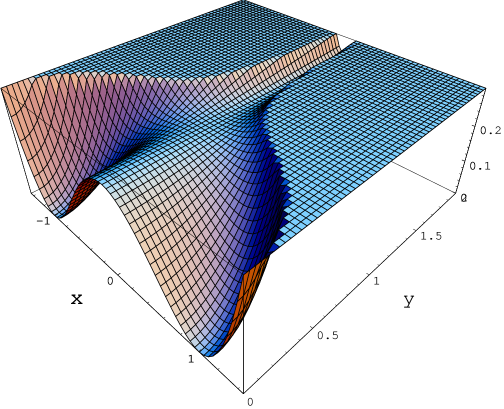
Figure 2: The potential close to the bifurcation point $x=0$,  $y=y_{b}=1/\sqrt{2}$.

In Fig. 2 we show the potential at $0\leq y\leq 2$ which details the approach to the bifurcation point: the local minimum becomes a maximum after passing $y_{b}$. In Fig. 3 we have potential at $0\leq y\leq y_{b}$ where one can see the transition of the flat potential into a maximum. In Fig. 4 we show the potential at $0\leq y\leq 0.3$, i.e. beyond the bifurcation point. It is clear here that close to $y=0$ we can see only the maximum of the potential at $x=0$ and an extremely unstable de Sitter space when coupled to gravity.

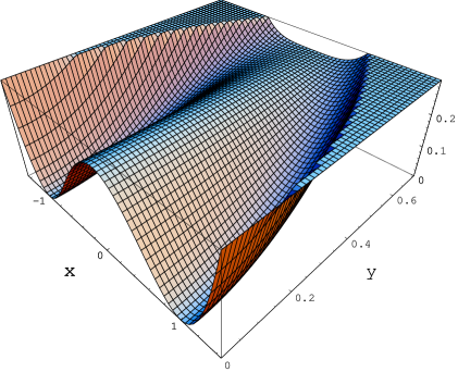
Figure 3: The potential is flat at the bifurcation point and has a maximum at $x=0$ and $y<y_{b}$.

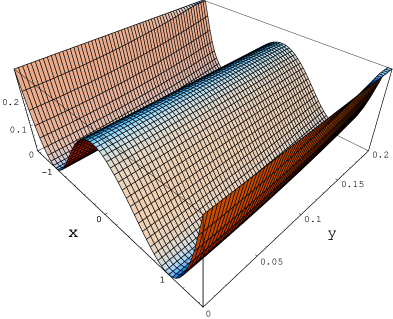
Figure 4: The potential beyond the bifurcation point shows a local maximum de Sitter stage, extremely unstable. The absolute ground state at $y=0$,  $x^{2}=1$ has 2 unbroken supersymmetries.

Figure 5: Slices of the potential of the hybrid hypersymmetric model, from $y=0$ to $y=10$. The lower curve corresponds to $y=0$. The curvature becomes positive for $y>1/\sqrt{2}$.

Finally, in Fig. 5 we have plotted the slices of the potentials at $y=10,2,y_{b},0.3,0$. The first 2 curves at $x=0$ have large positive curvature and positive potential, corresponding to the local de Sitter valley. At $y=y_{b}$ and $x=0$ the curvature is flat, the minimum is changing into the maximum, it is negative for $y=0.3$, $x=0$ and finally, at $y=0$ the curve reaches the vanishing value of the potential at $x^{2}=1$.

4 Coupling gauge theories to supergravity

4.1 Potentials of N=2 gauged supergravities

Coupling of N=2 supersymmetric gauge theories to supergravity was developed over the last 20 years, see for example [39, 40]. One would expect that at least in principle, any N=2 supersymmetric gauge theory can be coupled to N=2 supergravity. The opposite route, from gauged N=2 supergravity to a rigid N=2 gauge theories was developed in [40], where the proper limit of $M_{P}\rightarrow\infty$ was presented. In the recent investigations of superconformal symmetry, supergravity and cosmology in [41] it was found that such limit is greatly simplified in the context of the underlying superconformal theory.

More recently there was a renewal of the interest to gauged supergravities and their potentials in a search of domain wall solutions. The least understood part of N=2 gauged supergravities is a quaternionic part. Some new studies of the hypermultiplet structures of N=2 supergravities in [42, 43, 44, 45, 46] have revealed interesting features of the theory, which were not known before. Here we will give a short summary on this to the extent to which it is relevant to our search of de Sitter solutions in gauged N=2 supergravities.

Gauged N=2 supergravity with general interactions of vector multiplets and hypermultiplets is defined by some special Kähler and quaternionic geometries with some gauge isometries. The procedure of gauging involves the following major steps: i) the derivatives on the fields become covariant derivatives with the gauge coupling constant $g$ (different for each gauge group). These derivatives are defined in terms of Killing vectors related to isometries of the special Kähler and quaternionic manifolds, ii) for preservation the supersymmetry the action of ungauged supergravity after gauging has to be supplemented by two terms, the fermion ‘mass matrix’ and a potential. At $g=0$ all these terms disappear and ungauged supergravity is recovered. The potential can be presented as follows [40]:

$$V_{\rm supergr}^{N=2}=-3{\bar{L}}^{\Lambda}L^{\Sigma}P_{\Lambda}^{r}P_{\Sigma}^{r}+g^{2}(g^{i}{}_{j}k^{\Lambda i}k^{*j}_{\Sigma}+4h_{uv}k^{u}_{\Lambda}k^{v}_{\Sigma}){\bar{L}}^{\Lambda}L^{\Sigma}+g_{i}{}^{j}f^{\Lambda i}f^{*\Sigma}_{j}\sum_{r=1}^{r=3}P_{\Lambda}^{r}P_{\Sigma}^{r}\ .$$ (24)

Here $L^{\Lambda}(z,\bar{z})$ are the covariantly holomorphic sections of the special geometry, $f^{\Lambda i}=\nabla^{i}L^{\Lambda}$ and $P^{r}_{\Lambda}(z,\bar{z},q)$ are the triplets of the prepotentials for each gauge group. There are $n$ vector multiplets and a graviphoton from the supergravity multiplet, $\Lambda=0,1,\dots,n$. The potential is not positive definite, the first term, which was absent in the rigid case is negative definite. A useful form of the potential is given [43] in terms of a gravitino mass matrix of N=2 theory $S_{A}{}^{B}$ related to prepotential

$$L_{\rm gravitino}^{\rm mass}=2g\bar{\psi}^{A}_{\mu}S_{AB}\gamma^{\mu\nu}\psi_{\nu}^{B}\ ,\qquad S_{A}{}^{B}\equiv iP^{r}_{\Lambda}\sigma_{A}{}^{B}L^{\Lambda}\ .$$ (25)

The potential can be rewritten as follows:

$$V_{\rm supergr}^{N=2}=g^{2}[-6S_{AB}(S^{AB})^{*}+2g_{i}{}^{j}\nabla^{i}S_{AB}\nabla_{*j}(S^{AB})^{*}+4\nabla_{u}S_{AB}\nabla^{u}S_{AB}^{*}+g^{i}{}_{j}k_{i}k^{*j}]\ .$$ (26)

where $k_{i}=k_{i\Lambda}L^{\Lambda}$ and $k^{*j}=k^{*j}_{\Sigma}\bar{L}^{\Sigma}$. The negative definite contribution to the potential comes from the first term, the square of the gravitino mass term. The rest is positive definite, it includes the square of the derivatives over scalars of the special geometry as well as hypers and a terms with Killing vectors. This formula is quite intuitive and more easily associated with the formula for N=1 potential. In N=1 there is only one gravitino and therefore the mass matrix has just one element, ${W\over M_{P}^{2}}e^{K\over 2M_{P}^{2}}$. The negative contribution to the potential also comes from the gravitino mass term, see eq. (1). In the proper limit when $M_{P}\rightarrow\infty$ the gravitino mass vanishes and the potential of the rigid N=2 theory is positive definite.

Some examples of N=2 potentials will be studied in a separate publication [20]. The problem which we would like to address here is whether it is possible to couple hybrid hypersymmetric gauge theory to N=2 supergravity and preserve some nice features of the potential, discussed before.

4.2 FI terms and topological obstruction to couple hybrid hypersymmetry model to N=2 supergravity

The cosmologically interesting feature of the hybrid hypersymmetry model is due to the existence of the constant values of a component of a prepotential triplet in the $U(1)$ gauge theory.

It is a well known fact that in N=1 supersymmetry only in the abelian gauge group sector the theory can have constant FI D-terms. Adding a term linear in auxiliary field $D$ to the action would break gauge symmetry and supersymmetry. It will be useful for our purpose to explain this using a particular property of Kähler manifolds. The Killing vectors $k_{\Lambda i}$ on a Kähler manifolds are the derivatives of the Killing prepotentials $P_{\Lambda}$:

$$k_{\Lambda i}=ig_{i}{}^{j}\partial_{*j}P_{\Lambda}\ .$$ (27)

The prepotentials satisfy a Poisson bracket relation:

$$\{P_{\Lambda}\ ,P_{\Sigma}\}=f_{\Lambda\Sigma}^{\Gamma}P_{\Gamma}\ .$$ (28)

In the non-Abelian case this presents an obstruction to a possibility to add constant terms to the prepotentials. It also sets a precedent for us that a constant positive contribution to the potentials may be difficult to have in agreement with supersymmetries and gauge symmetries. In abelian case there is no problem since the eq. (28) has a vanishing right hand side,

$$\{P_{\Lambda}\ ,P_{\Sigma}\}=0\ .$$ (29)

and shift to a constant in any direction $\lambda$ does not contradict this relation.

Without the FI term, the SSF model of [33, 34] can be coupled to supergravity as it was done in [36, 39]. However, in presence of FI term there is so far no coupling to N=2 supergravity of this model available, to the best of our understanding. Moreover, we will present below the argument, that indicates that no such coupling may be possible in presence of constant $|P^{3}|=\xi$ terms.

To explain the argument we have to remind that the hypermultiplets of a rigid N=2 supersymmetry are associated with hyper-Kähler manifolds, whereas in N=2 supergravity they are associated with quaternionic manifolds [47]. A hyper-Kähler manifold has a flat $SU(2)$ curvature, and a quaternionic manifold has a non-vanishing $SU(2)$ curvature ${\cal R}^{r}_{uv}$. The relation between the Killing vectors of quaternionic manifolds $k^{v}_{\Lambda}$ and the triplets of the prepotentials $P^{r}_{\Lambda}$ known for a long time, see [48], is of the following nature:

$${\cal R}^{r}_{uv}k^{v}_{\Lambda}=D_{u}P^{r}_{\Lambda}\ ,\qquad k_{\Lambda}^{u}=-{4\over 3}{\cal R}^{r\,uv}D_{v}P^{r}_{\Lambda}\ .$$ (30)

Here $D_{u}$ is an $SU(2)$ covariant derivative over the quaternions

$$D_{u}P^{r}_{\Lambda}\equiv\partial_{u}P^{r}_{\Lambda}+2\varepsilon^{rst}\omega_{u}^{s}P^{t}_{\Lambda}\ ,$$ (31)

and the $SU(2)$ curvature is ${\cal R}^{r}=d\omega^{r}-\varepsilon^{rst}\omega^{s}\omega^{t}$. These prepotentials have recently been studied in a superconformal context in [38, 45]. The new relation which was found in [44] states that in local N=2 supersymmetry, i.e. in N=2 supergravity, the prepotentials are defined uniquely from the Killing vectors:

$$P^{r}_{\Lambda}={1\over 4n_{H}}D_{u}k_{\Lambda v}{\cal R}^{ruv}\ ,$$ (32)

where $n_{H}$ is the number of hypermultiplets. On the basis of this relation it has been concluded in [44] that any covariantly constant shift $P^{(0)r}_{\Lambda}$ is excluded since the integrability condition, $\varepsilon^{rst}{\cal R}^{suv}P^{(0)t_{\Lambda}}=0$ implies that $P^{(0)r}_{\Lambda}=0$. This implies the absence of the FI terms in all cases of N=2 supergravity with hypermultiplets. The exceptional cases when FI terms are possible, include theories with vector multiplets without hypermultiplets or cases of rigid supersymmetry when the curvature of the hyper-Kähler manifold vanishes. In both cases ${\cal R}^{r}_{uv}=0$ and FI terms are possible in agreement with supersymmetry and gauge symmetry. The confirmation of this analysis comes from the recently discovered [43] harmonicity property of the quaternionic prepotential

$$D^{u}D_{u}P^{r}_{\Lambda}=2n_{H}P^{r}_{\Lambda}\ .$$ (33)

This equation can be used to derive the equation (32). Thus in view of the properties of the quaternionic geometries explained above it looks plausible that the consistent coupling of hybrid hypersymmetric model with constant $\xi$ to N=2 supergravity is not possible. However, more investigations in this directions would be required to make a conclusive statement . The $SU(2,2|2)$ superconformal part of the model can be consistently coupled to N=2 supergravity, only the constant $\xi$-terms violating the superconformal symmetry seem to cause the problem .

4.3 Coupling of hybrid hypersymmetry model to N=1 supergravity

Coupling of hybrid hypersymmetric model with rigid N=2 supersymmetry to N=1 supergravity is simple. We may ignore the fact that the rigid limit has double supersymmetry and proceed as if only one supersymmetry is available and make it local. This procedure is of course not unique. The simplest one which we will also follow here was proposed in the context of D-term inflation in [26]. One can choose the minimal Kähler manifold for all 3 chiral superfields, two from the hypermultiplet, $\Phi_{1},\Phi_{2}$ and the one from the vector multiplet $\Phi_{3}$. In the Kähler geometry all 3 chiral multiplets now enter in a symmetric way. The D-terms will reflect that $\Phi_{1}$ and $\Phi_{2}$ have opposite charges and $\Phi_{3}$ is neutral. Also the kinetic term function $f$ of the vector multiplet may be taken minimal, i.e. field independent delta-function. Thus our N=1 supergravity has the Kähler potential, the superpotential and the potential given by

$$K=\sum_{a=1}^{a=3}|\Phi_{a}|^{2}\ ,\qquad W={g\over 6\sqrt{2}}\varepsilon^{abc}\Phi_{a}\Phi_{b}\Phi_{c}\ .$$ (34)

$$V = {g^{2}\over 8}e^{|\Phi_{a}|^{2}\over M_{P}^{2}}\left(\left[|\varepsilon^{abc}\Phi_{b}\Phi_{c}|\left(1+{|\Phi_{a}|^{2}\over M_{P}^{2}}\right)^{2}\right]^{2}-{1\over 3M_{P}^{2}}|\varepsilon^{abc}\Phi_{a}\Phi_{b}\Phi_{c}|^{2}\right)$$ (35)

$$+ {g^{2}\over 8}(|\Phi_{1}|^{2}-|\Phi_{2}|^{2}+{2\xi\over g})^{2}]\ .$$

Note the negative contribution due the term with the square of gravitino mass, $-3e^{K\over M_{P}^{2}}|W|^{2}$. Let us consider the critical points of this potential.

1. Non-supersymmetric de Sitter valley at some undefined but restricted constant value of the scalar $\Phi_{3}$, all hypers vanish.

$$|\Phi_{3}|=(|\Phi_{3}|)_{0}\ ,\qquad\Phi_{1}=\Phi_{2}=0\ ,\qquad W=0\ ,\qquad{\cal D}_{a}W=0\ ,$$ (36)

and

$$D=-\xi\ ,\qquad V={\xi^{2}\over 2}\ .$$ (37)

This is a local minimum of the potential, all supersymmetries are broken. Einstein equations have de Sitter solution. The possibility to have constant D-terms in N=1 supergravity was known for a long time. More recently a superconformal origin of FI terms was clarified in [41]. It was found there that the D-terms appear via the gauge transformation of the conformon multiplet, which plays an important role in the superconformal theory underlying supergravity.

2. Supersymmetric absolute global minimum

$$(\Phi_{3})_{\rm susy}=(\Phi_{1})_{\rm susy}=0\ ,\qquad W_{\rm susy}=0\ ,\qquad({\cal D}_{a}W)_{\rm susy}=0\ ,$$ (38)

and

$$D_{\rm susy}={g\over 2}|\Phi_{2}|^{2}_{\rm susy}-\xi=0\ ,\qquad V_{\rm susy}=0\ .$$ (39)

Thus the absolute minimum ground state has N=1 local supersymmetry unbroken and a vanishing potential. $U(1)$ gauge symmetry is spontaneously broken. Einstein equations at this vacuum have a solution with vanishing cosmological constant.

5 P-term inflation and acceleration of the universe

We will present here some short remarks about the applications in cosmology of N=2 supersymmetry with P-term inflation/acceleration, where $P^{r}$ is the triplet of the Killing prepotentials of N=2 gauge theory.

From our results we may conclude that at the tree level of N=2 supersymmetry of our model we have a de Sitter solution for $\Phi_{2}=0$ and for all sufficiently large values of the inflaton field $\Phi_{3}$. However for the cosmological solution we need to provide a slow roll regime so that inflation takes place. This issue has been analysed for D-term inflation in [26], and for P-term inflation the situation is very similar. It turns out that one can lift the flat direction of the inflaton field due to the first loop corrections in gauge theory. The tree level splitting of the masses in supermultiplets in de Sitter vacuum leads to the effective 1-loop potential for large inflaton field $\Phi_{3}$:

$$V_{1-\rm loop}={\xi^{2}\over 2}\Bigl{[}1+{g^{2}\over 8\pi^{2}}\ln{|\Phi_{3}^{2}|\over{|\Phi_{3}^{2}|_{c}}}+...\Bigr{]}.$$ (40)

This term is important because it leads to the motion of the field $\Phi_{3}$ towards the bifurcation point and the end of inflation. It is interesting to note that for the N= 2 P-term inflation, which corresponds to the N= 1 D-term inflation in the case $\lambda=\sqrt{2}\,g$ when this theory can be embedded into N=2 supersymmetric model, all non-gravitational higher loop corrections are finite [30].

As we already pointed out, even though our model is different from the F-term inflation, the effective potential of the fields $\Phi_{2}$ and $\Phi_{3}$ shown in Fig. 1 of our paper looks the same as in the simplest version of F-term inflation [24]. This theory has an interesting property. As one can see from Fig. 1, the potential near the bifurcation point has a very complicated shape. Thus one could expect that after the field $\Phi_{3}$ reaches the bifurcation point, both fields $\Phi_{2}$ and $\Phi_{3}$ will fall towards the minimum of the effective potential along a very complicated trajectory. This is indeed the case for the general D-term inflation models. Surprisingly enough, in the F-term model [24] the fields roll from the bifurcation point to the minimum of the effective potential along a straight line [49]. This simple behavior of the fields occurs in D-term inflation only for the particular case $\lambda=\sqrt{2}\,g$ corresponding to N= 2 P-term inflation: After inflation the fields $\Phi_{3}$ and $\Phi_{2}$ simultaneously oscillate along the straight line $\Phi_{2}+\sqrt{2}\Phi_{3}=\sqrt{\xi}$.

To study inflation in this theory one should use the Friedmann equation

$$H^{2}=\left({\dot{a}\over a}\right)^{2}=V/3\approx{\xi^{2}\over 6},$$ (41)

where $a(t)$ is a scale factor of the universe. Thus one has $H=\xi/\sqrt{6}$. This leads to inflation

$$a(t)=a(0)~{}\exp{{{\xi\ t\over\sqrt{6}}}}~{}.$$ (42)

For simplicity of notation, in the description of this stage we will write $\phi$ instead of $|\Phi_{3}|$. During the slow-roll regime the field $\phi=|\Phi_{3}|$ obeys equation $3H\dot{\phi}=-V^{\prime}(\phi)$ [3], which gives

$$\phi^{2}(t)=\phi^{2}(0)-{g^{2}\xi~{}t\over 2\sqrt{6}\pi^{2}}\ .$$ (43)

Suppose inflation ends soon after the field $\phi$ becomes smaller than $\phi_{c}=|\Phi_{3}|_{c}=\sqrt{\xi/g}$. This is a generic property of almost all versions of hybrid inflation [22]. Then using equations (42), (43) one can find the value of the field $\phi_{N}$ such that the universe inflates $e^{N}$ times when the field rolls from $\phi_{N}$ until it reaches the bifurcation point:

$$\phi_{N}^{2}={\phi_{c}}^{2}+{g^{2}N\over 2\pi^{2}}.$$ (44)

Density perturbations on the scale of the present cosmological horizon have been produced at $\phi\sim\phi_{N}$ with $N\sim 60$, and their amplitude is proportional to ${V^{3/2}\over V^{\prime}}$ at that time [3]. One can find parameters of our model using COBE normalization for inflationary perturbations of metric on the horizon scale [50, 28]:

$${V^{3/2}\over V^{\prime}}={2\sqrt{2}\pi^{2}\xi\over g}\phi_{N}\sim 5.3\times 10^{-4},$$ (45)

where $N\sim 60$. If ${\phi_{c}}^{2}={\xi\over g}\ll{g^{2}N\over 2\pi^{2}}$, one has $\phi_{N}={g\sqrt{N}\over\sqrt{2}\pi},$ and

$${V^{3/2}\over V^{\prime}}={2\pi\over g}{\xi\sqrt{N}}\sim 5.3\times 10^{-4}.$$ (46)

For $N\sim 60$ this implies that

$${\xi\over g}\approx 1.1\times 10^{-5}\ .$$ (47)

One can represent this result in terms of the amplitude of spontaneous symmetry breaking of gauge symmetry:

$$|\Phi_{2}|=\sqrt{2}|\Phi_{3}|_{c}=\sqrt{2\xi\over g}\approx 4.7\times 10^{-3}M_{p}\approx\ 1.1\times 10^{16}~{}{\rm GeV}.$$ (48)

This is very similar to the GUT scale.

It is worth mentioning that in addition to inflationary perturbations there may appear perturbations of metric created by cosmic strings that are formed after the end of inflation in this scenario [51, 22]. An investigation of this issue in the simplest versions of F-term and D-term inflation have shown that cosmic strings may lead to perturbations of metric proportional to $O({\xi/g})$. These perturbations can be of the same order of magnitude as inflationary perturbations or even few times greater [52, 50, 28]. If one wants to avoid the cosmic string contribution, one may suppress production of strings and other topological defects by making certain modifications to the model, see e.g. [53] and references therein. Alternatively, one may consider the models with very small $g^{2}$.

Indeed, the results described above have been obtained for $\phi_{c}^{2}={\xi\over g}\ll{g^{2}N\over 2\pi^{2}}\sim 3g^{2}$, i.e. for $g^{2}\gg 3\times 10^{-6}$. This is a natural assumption, but one should note that $g^{2}$ in our model is not related to the gauge coupling constant in GUTs, so it can be very small. In the regime $g^{2}<3\times 10^{-6}$ one has $\phi_{N}\approx\phi_{c}=\sqrt{\xi\over g}$, so that

$${V^{3/2}\over V^{\prime}}={2\sqrt{2}\pi^{2}\over g}\left({\xi\over g}\right)^{3/2}\sim 5.3\times 10^{-4}.$$ (49)

This yields

$${\xi\over g}\sim 0.7\times 10^{-4}~{}g^{2/3}.$$ (50)

For $g^{2}\ll 3\times 10^{-6}$ one has ${\xi\over g}\ll 10^{-5}$. This suppresses the cosmic string contribution to density perturbations while keeping the inflationary contribution intact.

In general, the hybrid hypersymmetry model can be used not only for inflation in the very early universe but also to explain the observed acceleration of the universe at the present epoch. Depending on the parameters of the theory and on initial conditions for the inflaton field $\Phi_{3}$, the universe may spend a very long time in de Sitter valley $\Phi_{2}=0$, $|\Phi_{3}|>\sqrt{\xi\over g}$. The bifurcation point may be approached very slowly but still within a finite time. When it is reached, as Figures 1-5 show, the waterfall stage will bring the universe to an absolute ground state with the vanishing cosmological constant and unbroken hypersymmetry. Recently it was argued that in a class of theories with a stable supersymmetric vacuum, a system cannot relax into a zero-energy supersymmetric vacuum while accelerating if the evolution is dominated by a single scalar field with a stable potential [15]. This was considered as a challenge for string theory as presently defined. In our model this problem does not appear: acceleration of the universe is not eternal, and the universe enters the state with unbroken supersymmetry due to the combined motion of two scalar fields.

One of the features of hybrid hypersymmetry model is that it requires at least 3 complex scalars: 1 complex scalar in a vector multiplet and a quaternion in a hypermultiplet. We were able to obtain de Sitter solution in N=2 theory only in presence of FI P-terms, which leads to hybrid inflation [22]. Thus hybrid inflation may appear to be the only mechanism for inflation/acceleartion consistent with N=2 supersymmetry.

We will show in [20] that all potentials available in the literature in N=2,4,8 gauged supergravities have de Sitter solutions which are either maxima or saddle points, in all cases highly unstable. However, most of the scalars in these gauged supergravities were truncated. Note that if one would take $|\Phi_{3}|<\sqrt{\xi\over g}$ in our N=2 model, one would also obtain only unstable solutions, as shown in Fig. 3,4. It is plausible that keeping more scalars (there are 35 complex scalars in N=8 theory) one can have a better chance to recover some hybrid-type potential with a long lasting de Sitter stage suitable for inflation and/or acceleration.

Another interesting possibility may be that the hybrid hypersymmetry gauge model with potential shown in Figures 1-5, may be directly related to string theory on $adS_{5}\times M^{5}$ space or to some stringy brane construction of the relevant gauge theory. This suggests that a further analysis of this and other theories with $N\geq 2$ supersymmetries may lead to interesting new links between M/string theory and cosmology.

I am grateful to O. Aharony, C. Herdeiro, S. Hirano, C. Hull, S. Kachru, L. Kofman, A. Linde, A. Maroto, S. Prokushkin, M. Shmakova, E. Silverstein, S. Susskind, S. Vandoren, A. Van Proeyen, P. West, B. de Wit and E. Witten for stimulating discussions. This work is supported by NSF grant PHY-9870115.

References

- [1] A.H. Guth, Phys. Rev. D23, 347 (1981); A.D. Linde, Phys. Lett. 108B, 389 (1982); A. Albrecht and P.J. Steinhardt, Phys. Rev. Lett. 48, 1220 (1982); A.D. Linde, Phys. Lett. 129B, 177 (1983).
- [2] P. de Bernardis et al, “Multiple Peaks in the Angular Power Spectrum of the Cosmic Microwave Background: Significance and Consequences for Cosmology,” astro-ph/0105296; M. S. Turner,“Dark energy and the new cosmology,” astro-ph/0108103.
- [3] A.D. Linde, Particle Physics and Inflationary Cosmology (Harwood Academic Publishers, Chur, Switzerland 1990).
- [4] N. Weiss, “Possible Origins Of A Small Nonzero Cosmological Constant,” Phys. Lett. B 197, 42 (1987); C. Wetterich, “Cosmology and Fate of Dilatation Symmetry”, Nucl. Phys. B 302, 668 (1988); B. Ratra and P. J. Peebles, “Cosmological Consequences Of A Rolling Homogeneous Scalar Field,” Phys. Rev. D 37, 3406 (1988); P. G. Ferreira and M. Joyce, “Structure formation with a self-tuning scalar field,” Phys. Rev. Lett. 79, 4740 (1997) [astro-ph/9707286]; R. R. Caldwell, R. Dave and P. J. Steinhardt, “Cosmological Imprint of an Energy Component with General Equation-of-State,” Phys. Rev. Lett. 80, 1582 (1998) [astro-ph/9708069].
- [5] S. Ferrara, “Algebraic Properties Of Extended Supergravity In De Sitter Space,” Phys. Lett. B 69, 481 (1977).
- [6] G. W. Gibbons, “Aspects Of Supergravity Theories,” Print-85-0061 (CAMBRIDGE) Three lectures given at GIFT Seminar on Theoretical Physics, San Feliu de Guixols, Spain, Jun 4-11, 1984.
- [7] K. Pilch, P. van Nieuwenhuizen and M. F. Sohnius, “De Sitter Superalgebras And Supergravity,” Commun. Math. Phys. 98, 105 (1985).
- [8] S. J. Gates and B. Zwiebach, “Gauged N=4 Supergravity Theory With A New Scalar Potential,” Phys. Lett. B 123, 200 (1983).
- [9] C. M. Hull and N. P. Warner, “The Potentials Of The Gauged N=8 Supergravity Theories,” Nucl. Phys. B 253, 675 (1985).
- [10] T. Banks, “Cosmological breaking of supersymmetry or little Lambda goes back to the future. II,” arXiv:hep-th/0007146.
- [11] J. Maldacena and C. Nunez, “Supergravity description of field theories on curved manifolds and a no go theorem,” Int. J. Mod. Phys. A 16, 822 (2001) [hep-th/0007018].
- [12] R. Bousso, JHEP 0011, 038 (2000) [arXiv:hep-th/0010252].
- [13] T. Banks and W. Fischler, “M-theory observables for cosmological space-times,” [hep-th/0102077].
- [14] E. Witten, “Quantum gravity in de Sitter space,” [hep-th/0106109].
- [15] S. Hellerman, N. Kaloper and L. Susskind, “String theory and quintessence,” JHEP 0106, 003 (2001) [hep-th/0104180].
- [16] W. Fischler, A. Kashani-Poor, R. McNees and S. Paban, “The acceleration of the universe, a challenge for string theory,” JHEP 0107, 003 (2001) [hep-th/0104181].
- [17] M. Spradlin, A. Strominger and A. Volovich, “Les Houches lectures on de Sitter space,” arXiv:hep-th/0110007.
- [18] C. M. Hull, “de Sitter space in supergravity and M theory,” arXiv:hep-th/0109213.
- [19] P. K. Townsend, “Quintessence from M-theory,” arXiv:hep-th/0110072.
- [20] R. Kallosh, A. D. Linde, S. Prokushkin and M. Shmakova, “Gauged supergravities, de Sitter space and cosmology,” arXiv:hep-th/0110089.
- [21] J. Garcia-Bellido, Phys. Lett. B 418, 252 (1998) [arXiv:hep-th/9707059].
- [22] A. D. Linde, “Axions in inflationary cosmology,” Phys. Lett. B 259, 38 (1991). A. D. Linde, “Hybrid inflation,” Phys. Rev. D 49, 748 (1994) [astro-ph/9307002].
- [23] E. J. Copeland, A. R. Liddle, D. H. Lyth, E. D. Stewart and D. Wands, “False vacuum inflation with Einstein gravity,” Phys. Rev. D 49, 6410 (1994) [astro-ph/9401011];
- [24] G. R. Dvali, Q. Shafi and R. Schaefer, “Large scale structure and supersymmetric inflation without fine tuning,” Phys. Rev. Lett. 73, 1886 (1994) [hep-ph/9406319].
- [25] E. D. Stewart, “Inflation, supergravity and superstrings,” Phys. Rev. D 51, 6847 (1995) [hep-ph/9405389].
- [26] P. Binetruy and G. Dvali, “D-term inflation,” Phys. Lett. B 388, 241 (1996) [hep-ph/9606342].
- [27] E. Halyo, “Hybrid inflation from supergravity D-terms,” Phys. Lett. B 387, 43 (1996) [hep-ph/9606423].
- [28] D. H. Lyth and A. Riotto, “Particle physics models of inflation and the cosmological density perturbation,” Phys. Rept. 314, 1 (1999) [hep-ph/9807278].
- [29] E. Halyo, “Hybrid quintessence with an end or quintessence from branes and large dimensions,” [hep-ph/0105216].
- [30] M. T. Grisaru and W. Siegel, “Supergraphity. 2. Manifestly Covariant Rules And Higher Loop Finiteness,” Nucl. Phys. B 201, 292 (1982) [Erratum-ibid. B 206, 496 (1982)]; P. S. Howe, K. S. Stelle and P. C. West, “A Class Of Finite Four-Dimensional Supersymmetric Field Theories,” Phys. Lett. B 124, 55 (1983); P. S. Howe, K. S. Stelle and P. K. Townsend, “Miraculous Ultraviolet Cancellations In Supersymmetry Made Manifest,” Nucl. Phys. B 236, 125 (1984).
- [31] E. Cremmer, S. Ferrara, L. Girardello and A. Van Proeyen, “Yang-Mills Theories With Local Supersymmetry: Lagrangian, Transformation Laws And Superhiggs Effect,” Nucl. Phys. B 212, 413 (1983).
- [32] M. F. Sohnius, “Introducing Supersymmetry,” Phys. Rept. 128, 39 (1985).
- [33] A. Salam and J. Strathdee, “Supersymmetry, Parity And Fermion - Number Conservation,” Nucl. Phys. B 97, 293 (1975).
- [34] P. Fayet, “Fermi-Bose Hypersymmetry,” Nucl. Phys. B 113, 135 (1976).
- [35] N. Seiberg and E. Witten, “Monopoles, duality and chiral symmetry breaking in N=2 supersymmetric QCD,” Nucl. Phys. B 431, 484 (1994) [hep-th/9408099].
- [36] B. de Wit, J. W. van Holten and A. Van Proeyen, “Central Charges And Conformal Supergravity,” Phys. Lett. B 95, 51 (1980).
- [37] P. West, “Introduction To Supersymmetry And Supergravity,” Singapore, Singapore: World Scientific (1990) 425 p.
- [38] B. de Wit, B. Kleijn and S. Vandoren, “Rigid N = 2 superconformal hypermultiplets,” arXiv:hep-th/9808160; B. de Wit, B. Kleijn and S. Vandoren, “Superconformal hypermultiplets,” Nucl. Phys. B 568, 475 (2000) [arXiv:hep-th/9909228].
- [39] B. de Wit, P. G. Lauwers and A. Van Proeyen, “Lagrangians Of N=2 Supergravity - Matter Systems,” Nucl. Phys. B 255, 569 (1985).
- [40] L. Andrianopoli, M. Bertolini, A. Ceresole, R. D’Auria, S. Ferrara and P. Fre’, “General Matter Coupled N=2 Supergravity,” Nucl. Phys. B 476, 397 (1996) [hep-th/9603004].
- [41] R. Kallosh, L. Kofman, A. D. Linde and A. Van Proeyen, “Superconformal symmetry, supergravity and cosmology,” Class. Quant. Grav. 17, 4269 (2000) [hep-th/0006179].
- [42] B. de Wit, M. Rocek and S. Vandoren, “Hypermultiplets, hyperkaehler cones and quaternion-Kaehler geometry,” JHEP 0102, 039 (2001) [arXiv:hep-th/0101161].
- [43] R. D’Auria and S. Ferrara, “On fermion masses, gradient flows and potential in supersymmetric theories,” JHEP 0105, 034 (2001) [hep-th/0103153].
- [44] A. Ceresole, G. Dall’Agata, R. Kallosh and A. Van Proeyen, “Hypermultiplets, domain walls and supersymmetric attractors,” [hep-th/0104056].
- [45] B. de Wit, M. Rocek and S. Vandoren, “Gauging isometries on hyperKaehler cones and quaternion-Kaehler manifolds,” Phys. Lett. B 511, 302 (2001) [arXiv:hep-th/0104215].
- [46] D. V. Alekseevsky, V. Cortes, C. Devchand and A. V. Proeyen, “Flows on quaternionic-Kaehler and very special real manifolds,” [hep-th/0109094].
- [47] J. Bagger and E. Witten, “Matter Couplings In N=2 Supergravity ,” Nucl. Phys. B 222, 1 (1983).
- [48] K. Galicki, “A Generalization Of The Momentum Mapping Construction For Quaternionic Kahler Manifolds,” Commun. Math. Phys. 108, 117 (1987).
- [49] M. Bastero-Gil, S. F. King and J. Sanderson, “Preheating in supersymmetric hybrid inflation,” Phys. Rev. D 60, 103517 (1999) [hep-ph/9904315].
- [50] A. D. Linde and A. Riotto, “Hybrid inflation in supergravity,” Phys. Rev. D 56, 1841 (1997) [arXiv:hep-ph/9703209].
- [51] L. A. Kofman and A. D. Linde, “Generation Of Density Perturbations In The Inflationary Cosmology,” Nucl. Phys. B 282, 555 (1987).
- [52] R. Jeannerot, “Inflation in supersymmetric unified theories,” Phys. Rev. D 56, 6205 (1997) [arXiv:hep-ph/9706391]; C. Contaldi, M. Hindmarsh and J. Magueijo, “CMB and density fluctuations from strings plus inflation,” Phys. Rev. Lett. 82, 2034 (1999) [arXiv:astro-ph/9809053]; R. A. Battye and J. Weller, “Cosmic structure formation in hybrid inflation models,” Phys. Rev. D 61, 043501 (2000) [arXiv:astro-ph/9810203]; F. R. Bouchet, P. Peter, A. Riazuelo and M. Sakellariadou, “Is there evidence for topological defects in the BOOMERANG data?,” arXiv:astro-ph/0005022; C. R. Contaldi, “Cosmic strings in the age of Boomerang,” arXiv:astro-ph/0005115.
- [53] G. Lazarides, “Supersymmetric hybrid inflation,” arXiv:hep-ph/0011130.